Genome-wide Determination Of Splicing Efficiency And ...

Genome-wide Determination Of

Splicing Efficiency And Dynamics

From RNA-Seq Data

Dissertation zur Erlangung des Grades eines Doktors der

Naturwissenschaften (Dr. rer. nat.) vorgelegt von

Verônica Rodrigues de Melo Costa

am Fachbereich Mathematik und Informatik

der Freien Universität Berlin

Berlin, 2020

Gutachter:

Prof. Dr. Martin Vingron, Freie Universität Berlin, Deutschland (1. Gutachter)

Prof. Dr. Rosario M. Piro

Datum der Disputation: 22\04\2021

i

Abstract

Eukaryotic genes are mostly composed of a series of exons intercalated by sequences with no

coding potential called introns. These sequences are generally removed from primary

transcripts to form mature RNA molecules in a post-transcriptional process called splicing. An

efficient splicing of primary transcripts is an essential step in gene expression and its

misregulation is related to numerous human diseases. Thus, to better understand the dynamics

of this process and the perturbations that might be caused by aberrant transcript processing, it

is important to quantify splicing efficiency. In this thesis, I introduce SPLICE-q, a fast and

user-friendly Python tool for genome-wide SPLICing Efficiency quantification. It supports

studies focusing on the implications of splicing efficiency in transcript processing dynamics.

SPLICE-q uses aligned reads from RNA-Seq to quantify splicing efficiency for each intron

individually and allows the user to select different levels of restrictiveness concerning the

introns’ overlap with other genomic elements, such as exons from other genes. I demonstrate

SPLICE-q’s application using three use cases including two different species and

methodologies. These analyses illustrate that SPLICE-q can detect a progressive increase of

splicing efficiency throughout a time course of nascent RNA-Seq and it might be useful when

it comes to understanding cancer progression beyond mere gene expression levels.

Furthermore, I provide an in-depth study of time course nascent BrU-Seq data to address

questions concerning differences in the speed of splicing and the underlying biological features

that might be associated with it. SPLICE-q and its documentation are publicly available at:

https://github.com/vrmelo/SPLICE-q.

ii

Preface

This thesis is an original work by Verônica Rodrigues de Melo Costa and it will provide a

detailed study on RNA splicing kinetics and dynamics developed over the course of five years.

The work is divided into Introduction, Materials and Methods, Results, Discussion and

Conclusion. In detail, Chapter I contains a detailed introduction of the basic concepts of

molecular biology focusing mainly on pre-mRNA splicing, its regulatory mechanisms, and

how its misregulation impacts the functionality of the cell. It also introduces RNA sequencing

and its key applications, and what and how bioinformatics approaches can be applied to better

understand splicing; Chapter II describes the materials and methods for the study, including

details on the tools and algorithms used; Chapter III introduces the approach used to develop

SPLICE-q, an up-to-date and user-friendly tool for splicing efficiency quantification; Chapter

IV shows the usefulness of SPLICE-q by applying it to various datasets; Chapter V consists

of an in-depth study addressing questions concerning the differences in the speed of splicing

and the underlying biological features that might be associated with it; and Chapter VI

provides a detailed discussion of the most prominent results and a conclusion. Portions of

Chapters III and IV have been published as: V. R. Melo Costa, J. Pfeuffer, A. Louloupi, U. A.

V Ørom, and R. M. Piro, “SPLICE-q: a Python tool for genome-wide quantification of splicing

efficiency,” bioRxiv, p. 2020.10.12.318808, Oct. 2020.

iii

Acknowledgments

I am very grateful to so many people, who have been directly or indirectly essential in getting

this thesis finished. Some, however, should be named:

A big thank you to my supervisor Dr. Rosario M. Piro for his guidance, feedbacks and patience

during this research. Thank you to Drs. Martin Vingron, Evgenia Ntini and Ulf A. Orom for

fruitful discussions in different stages of this project. I would like to express my gratitude and

appreciation to Dr. Kirsten Kelleher for being one of the greatest supports I had throughout

these years. Many thanks to Dr. Knut Reinert, Anja Kasseckert and colleagues from the ABI

group for being so welcoming. I will miss our coffee times! I am also very grateful to all my

friends, who always made me feel loved and confident, but specially: Drs. Katia Paiva,

Henrique Assis and Ricardo Vialle; Dr. Tiago B. Castro; Deborah Delbue and Danielle

Cardoso; Michael Sidwell; Michele Pugini, Claudia Romanini and Lidiane Morafka; and so

many more. I am very lucky to have you all in my life! Thank you to Julianus Pfeuffer for his

unconditional support in this very intense journey. You made everything worth it! And finally,

a huge thank you to my family, specially my mom, dad and brother, who set me off on this

academic road a long time ago and to whom I dedicate this work. Your love and encouragement

made this happen!

The initial years of this PhD were funded by Coordenação de Aperfeiçoamento de Pessoal de

Nível Superior (CAPES).

iv

Table of Contents

Abstract ....................................................................................................................................... i

Preface........................................................................................................................................ ii

Acknowledgments.................................................................................................................... iii

Table of contents ....................................................................................................................... iv

List of figures ......................................................................................................................... viii

List of tables and boxes............................................................................................................. ix

CHAPTER I. INTRODUCTION ........................................................................................... 1

1. The eukaryotic gene .............................................................................................................. 3

2. From DNA to RNA: A short overview of DNA transcription .............................................. 5

3. RNA secondary structure ...................................................................................................... 7

4. Post-transcriptional modifications ......................................................................................... 9

4.1. RNA capping ................................................................................................................ 9

4.2. 3’ end formation: The poly(A) tail................................................................................ 9

4.3. The landscape of splicing............................................................................................ 10

4.3.1. The biochemistry of splicing ............................................................................. 10

4.3.2. Small nuclear ribonucleoprotein particles ......................................................... 12

4.3.3. Spliceosome assembly and activity ................................................................... 13

4.3.4. Alternative splicing: increasing the diversity of the proteome .......................... 15

4.3.5. Crosstalk between transcription and splicing .................................................... 17

4.3.6. Defective pre-mRNA splicing ........................................................................... 18

5. Splicing kinetics: How to get there? .................................................................................... 19

5.1. Experimental tracing of splicing kinetics ................................................................... 20

5.2. Measurement of splicing efficiency using RNA-Seq reads ........................................ 22

6. Objectives and Significance ............................................................................................... 23

CHAPTER II. MATERIALS & METHODS ...................................................................... 26

1. Cell culture and metabolic labeling ..................................................................................... 26

1.1. RNA-Seq data processing and QC .............................................................................. 27

2. Other datasets ...................................................................................................................... 27

3. Clustering ............................................................................................................................ 28

3.1. K-means ...................................................................................................................... 28

v

3.2. Hierarchical clustering ................................................................................................ 29

4. Gene type annotation ........................................................................................................... 29

5. Gene expression quantification .......................................................................................... 30

6. Motif enrichment analysis (MEA) ...................................................................................... 31

6.1. Transcription start sites (TSS) .................................................................................... 31

6.2. RNA-binding proteins (RBPs) .................................................................................... 32

6.2.1. Splicing factors .................................................................................................. 33

7. Analysis of splice site strength ............................................................................................ 33

8. RBP preferences for secondary structure ............................................................................ 34

CHAPTER III. RESULTS: SPLICE-q ............................................................................... 35

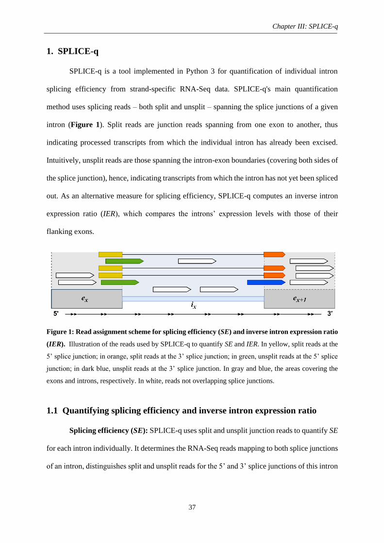
1. SPLICE-q ............................................................................................................................. 37

1.1. Quantifying splicing efficiency and inverse intron expression ratio .......................... 37

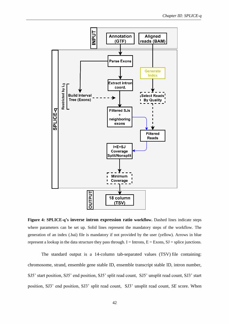
1.2. Workflow and parameters ........................................................................................... 39

1.3. Compatibility and requirements .................................................................................. 44

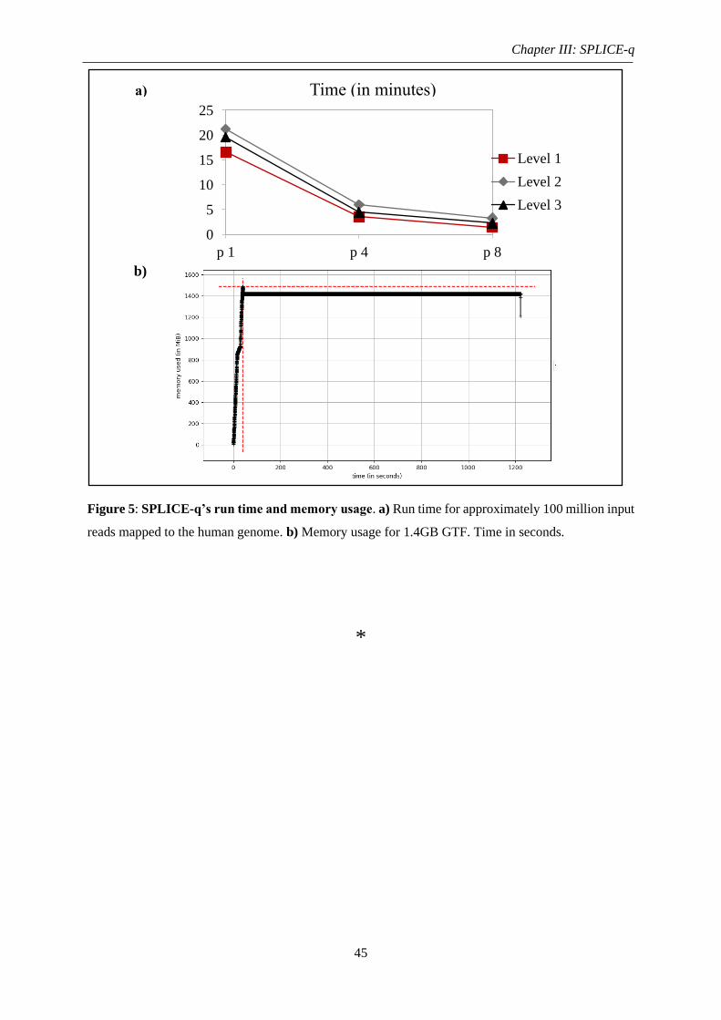
1.4. Fast and user-friendly quantification of splicing efficiency ....................................... 44

CHAPTER IV. RESULTS: SPLICE-q APPLICATION .................................................. 46

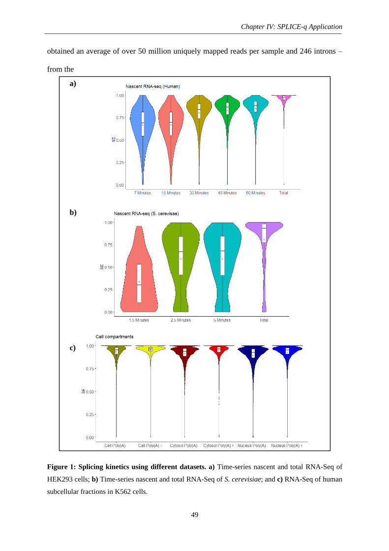
1. Splicing kinetics of human and yeast................................................................................... 48

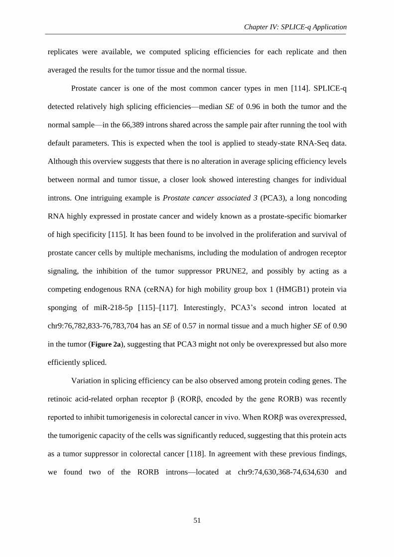
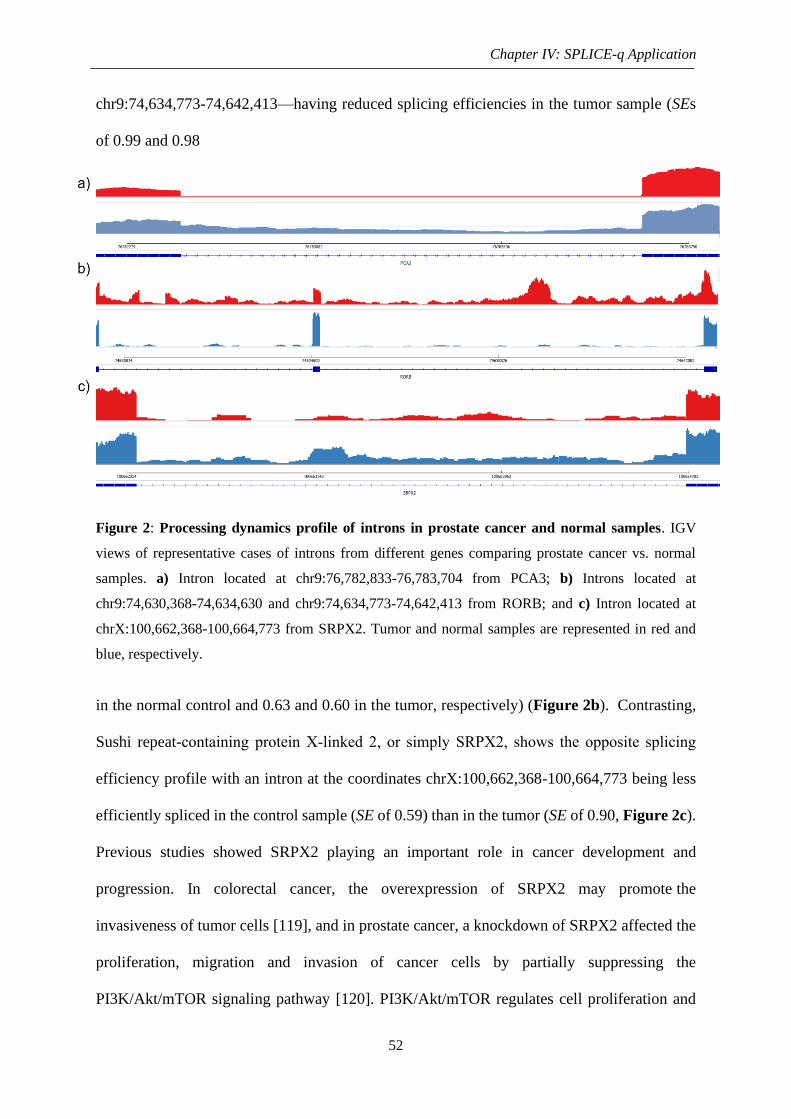
2. Analysis of prostate cancer data .......................................................................................... 50

CHAPTER V. RESULTS: SPLICING DYNAMICS ........................................................ 54

1. Dataset and clustering step.................................................................................................. 56

2. Biological features .............................................................................................................. 59

2.1. Gene architecture ........................................................................................................ 59

2.1.1. Length and nucleotide composition ................................................................... 59

2.1.2. Intron ordinal position........................................................................................ 61

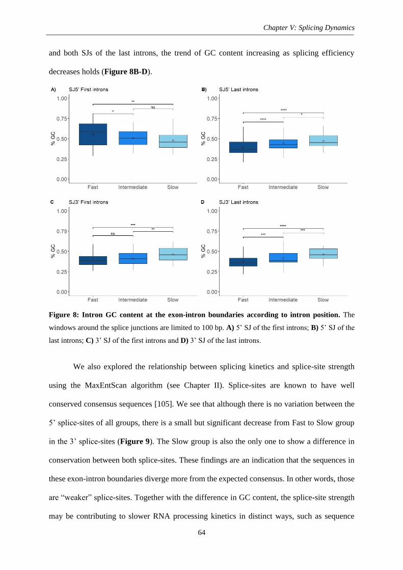
2.2. Splice junctions ........................................................................................................... 63

2.2.1. Donor-acceptor consensus sequences ................................................................ 65

3. Motif enrichment analysis................................................................................................... 66

3.1. Transcription start sites ............................................................................................... 64

3.2. RBPs in the intronic regions ....................................................................................... 69

3.2.1. Fast splicing ....................................................................................................... 69

3.2.2. Slow splicing ...................................................................................................... 71

3.3. RNA structural elements ............................................................................................. 72

CHAPTER VI. DISCUSSION . ............................................................................................ 76

1. Discussion ........................................................................................................................... 77

vi

1.1. SPLICE-q facilitates the quantification of splicing efficiency ................................... 77

1.2. SPLICE-q can be applied to different types of RNA-Seq .......................................... 78

1.3. SE values revealed different patterns of splicing over a time course ......................... 79

1.4. Splicing dynamics depend on biological features ....................................................... 80

1.4.1. Gene architecture and splicing speed ................................................................. 80

1.4.2. Splicing differences between coding and non-coding genes ............................. 81

1.4.3. Importance of regulatory RNA motifs and secondary structure ........................ 82

2. Conclusion ........................................................................................................................... 83

Glossary ................................................................................................................................... 85

References ................................................................................................................................ 86

Zusammenfassung.................................................................................................................... 98

Eigenständigkeitserklärung ...................................................................................................... 99

vii

List of Figures


Figure 1: Structure of a protein coding gene ............................................................................. 5

Figure 2: Representation of RNA secondary structures ............................................................ 8

Figure 3: Transesterification reactions in pre-mRNA splicing ................................................ 11

Figure 4: snRNP complexes..................................................................................................... 13

Figure 5: U2-type spliceosome assembly and activity ............................................................ 14

Figure 6: Constitutive and alternative splicing ........................................................................ 16

Figure 7: Standard RNA-Seq protocol ..................................................................................... 21


Figure 1: Cell culture and metabolic labeling .......................................................................... 26

CHAPTER III: SPLICE-q .................................................................................................... 35

Figure 1: Read assignment scheme for splicing efficiency (SE) and inverse intron expression

ratio (IER) ................................................................................................................................ 37

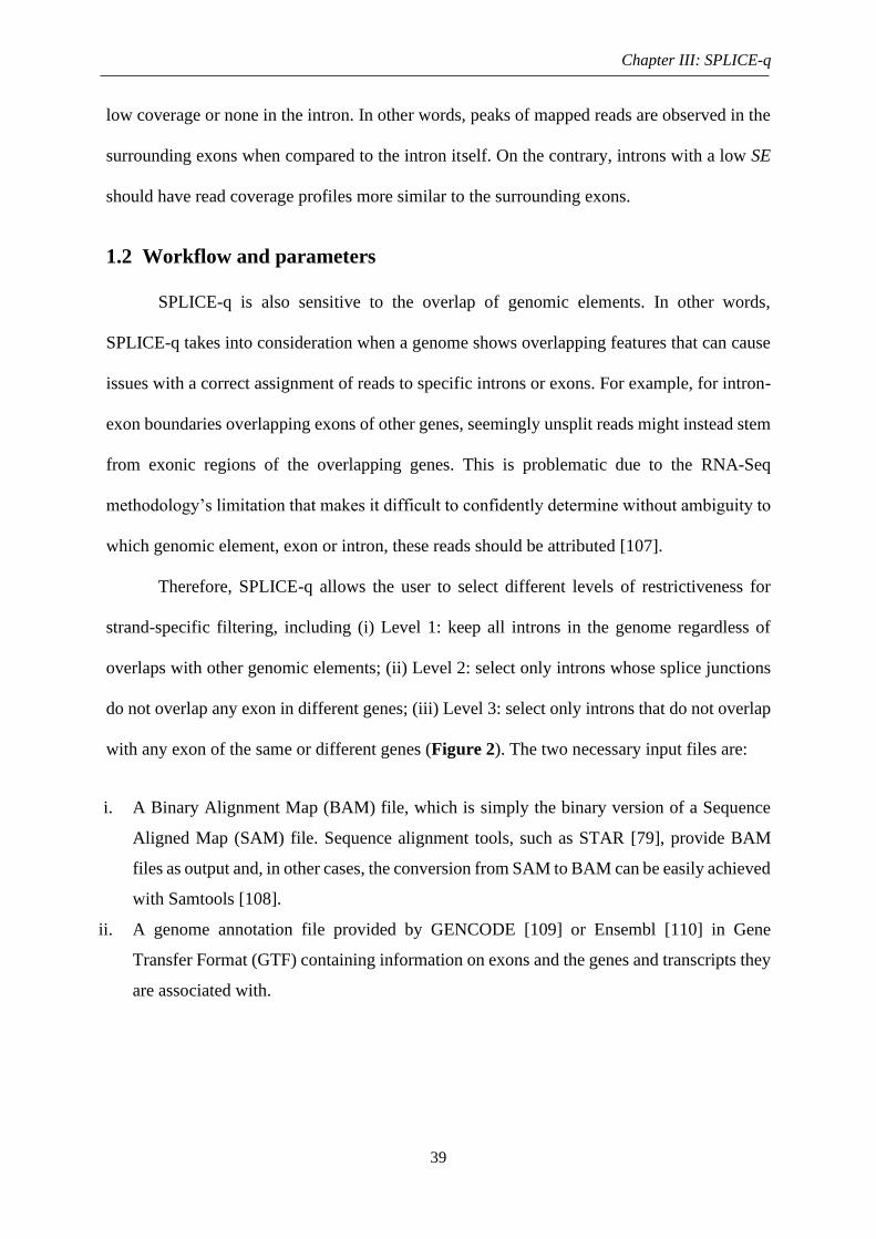
Figure 2: SPLICE-q’s levels of restrictiveness ........................................................................ 40

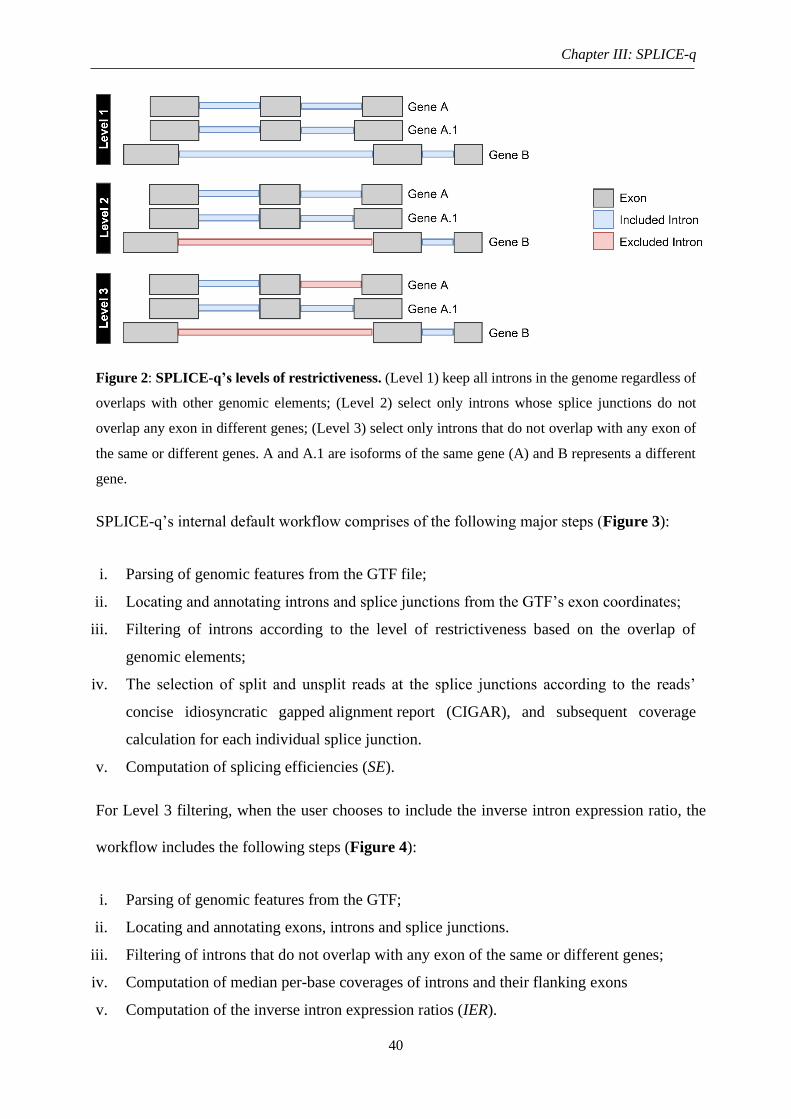
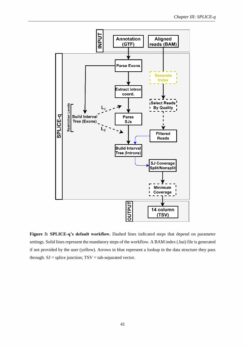
Figure 3: SPLICE-q’s default workflow .................................................................................. 41

Figure 4: SPLICE-q’s inverse intron expression ratio workflow ............................................ 42

Figure 5: SPLICE-q’s run time and memory usage ................................................................. 45

CHAPTER IV. SPLICING KINETICS ............................................................................... 46

Figure 1: Splicing kinetics using different datasets ................................................................. 49

Figure 2: Processing dynamics profile of introns in prostate cancer and normal samples. ..... 52

CHAPTER V: SPLICING DYNAMICS ............................................................................. 54

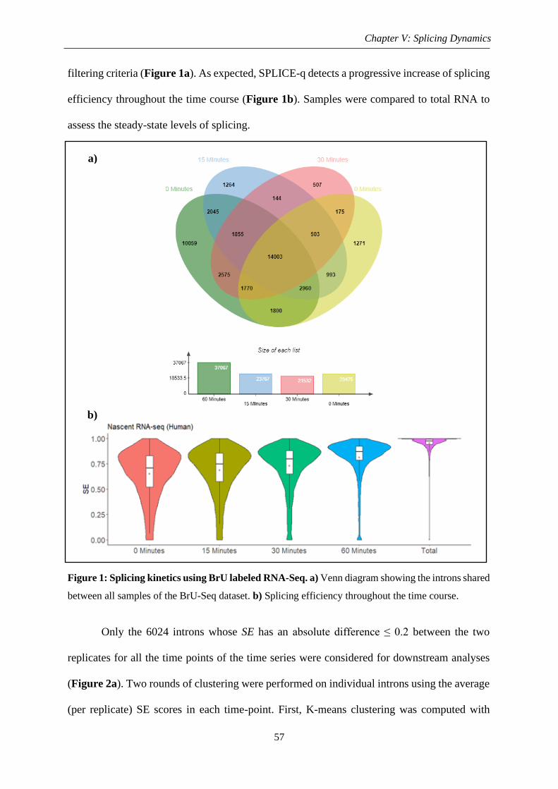
Figure 1: Splicing kinetics using BrU labeled RNA-Seq ........................................................ 57

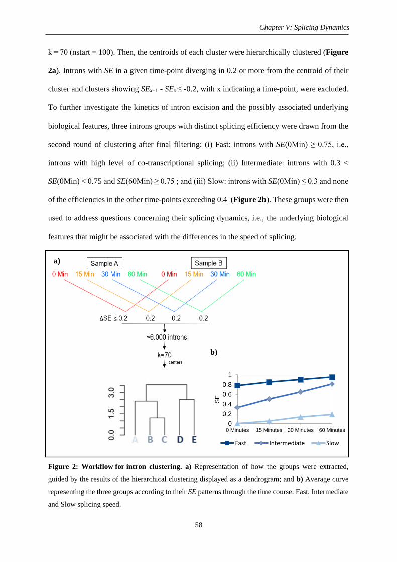
Figure 2: Workflow for intron clustering ................................................................................. 58

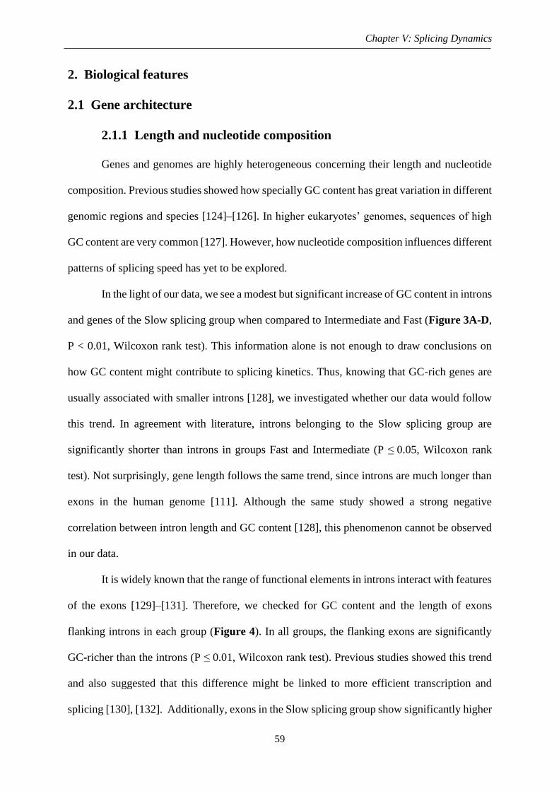
Figure 3: Gene and intron nucleotide composition and length ................................................ 60

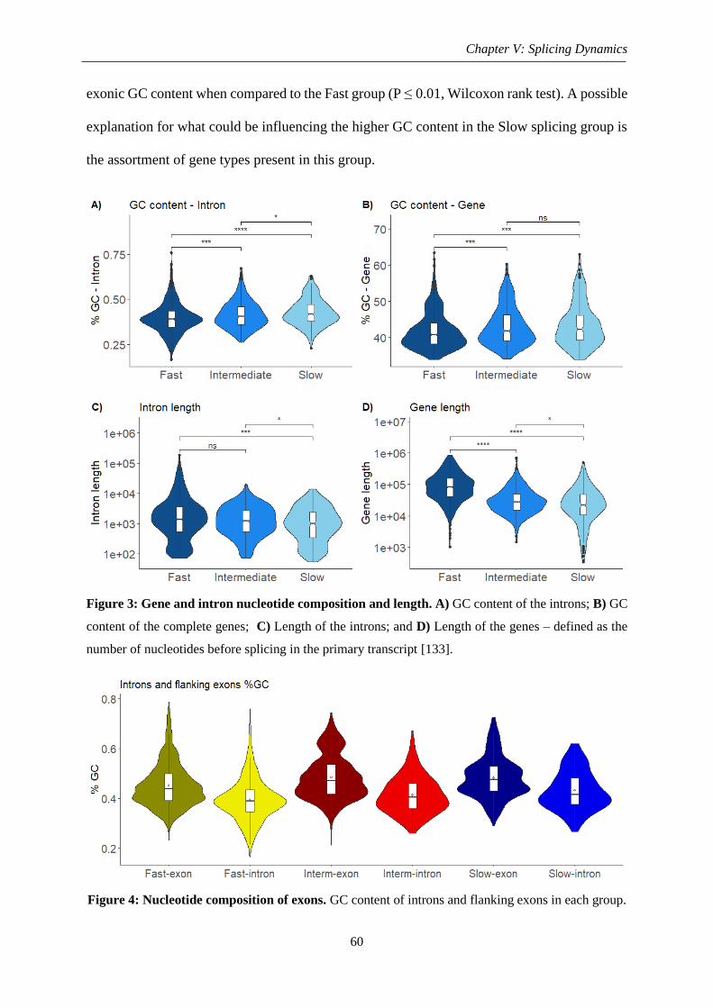
Figure 4: Nucleotide composition of exons ............................................................................. 60

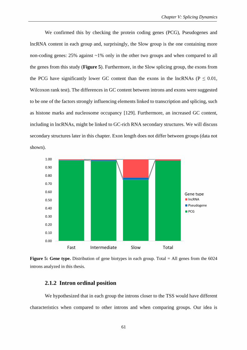
Figure 5: Gene type .................................................................................................................. 61

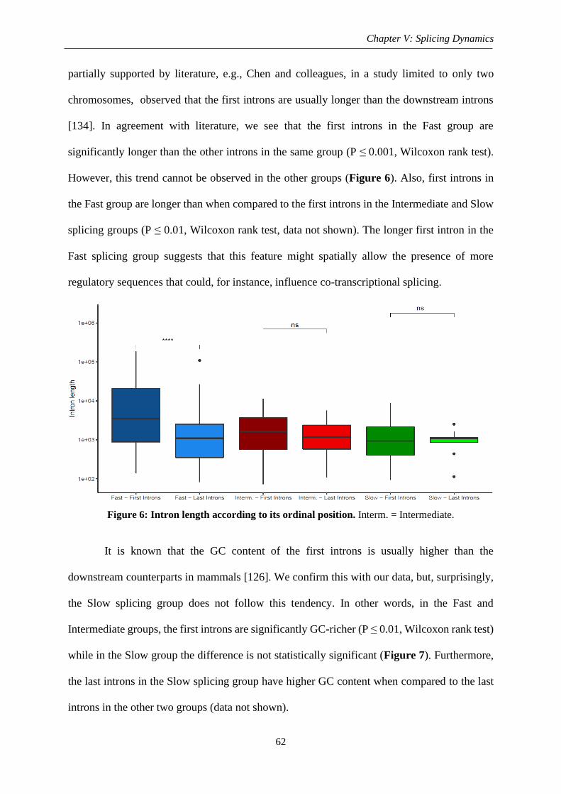
Figure 6: Intron length according to its ordinal position ......................................................... 62

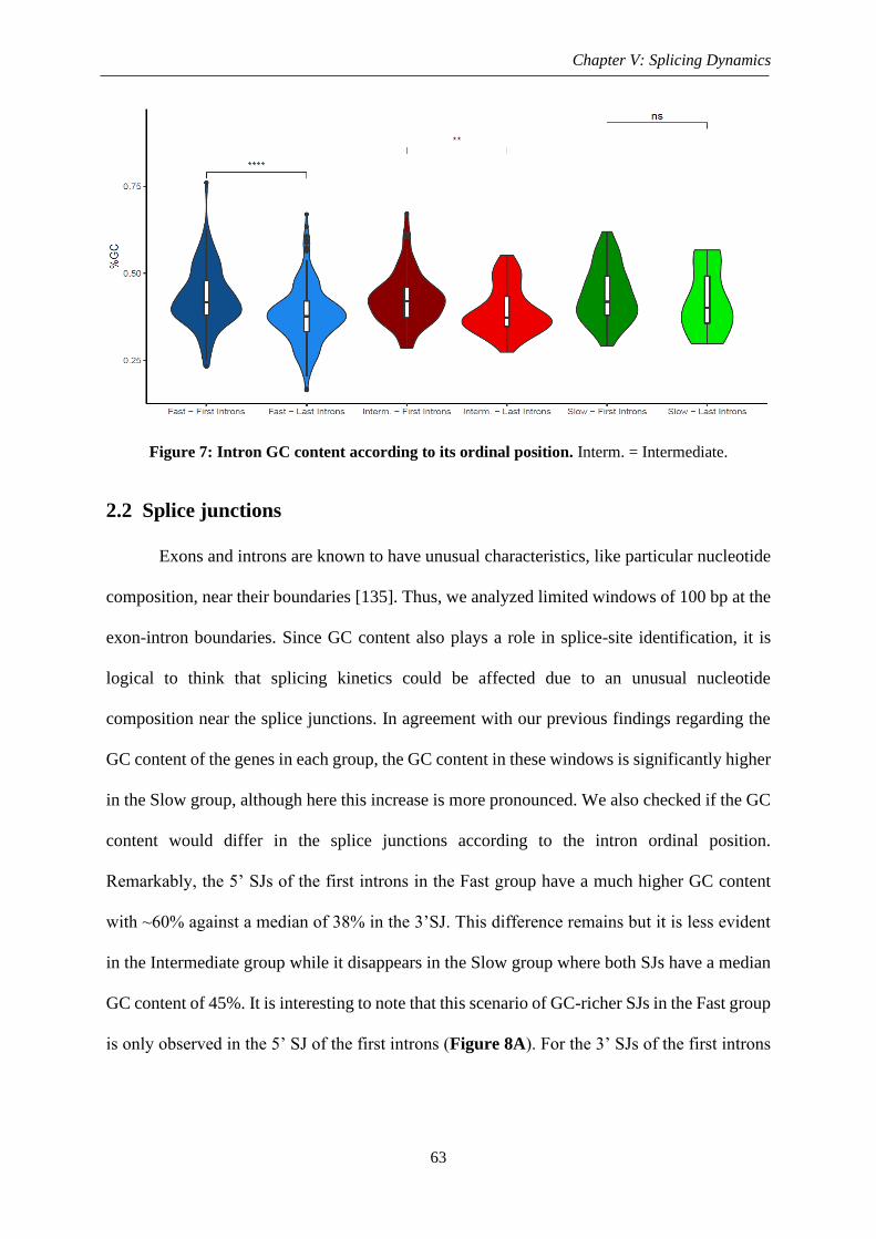
Figure 7: Intron GC content according to its ordinal position ................................................. 63

Figure 8: Intron GC content at the exon-intron boundaries according to intron position ........ 64

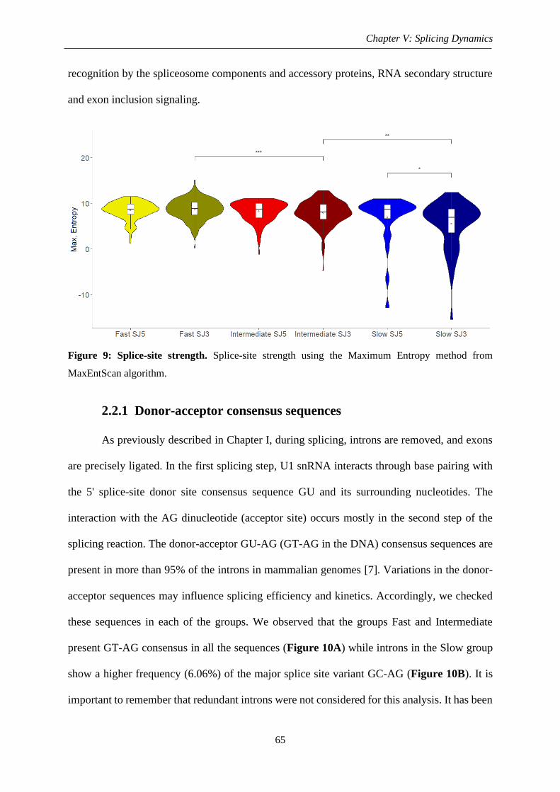
Figure 9: Splice-site strength ................................................................................................... 65

Figure 10: Consensus sequences at donor and acceptor splice-sites ....................................... 66

viii

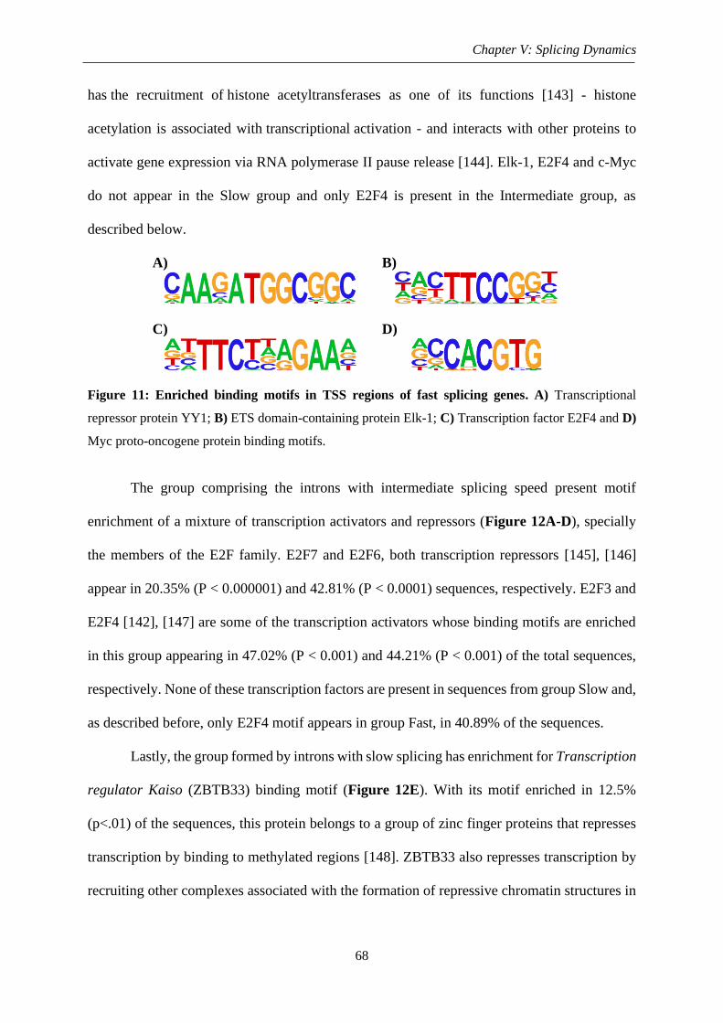
Figure 11: Enriched binding motifs in TSS regions of fast splicing genes ............................. 68

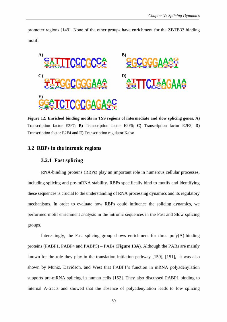
Figure 12: Enriched binding motifs in TSS regions of intermediate and slow splicing genes 69

Figure 13: Enriched binding motifs in intronic regions of fast splicing genes ........................ 70

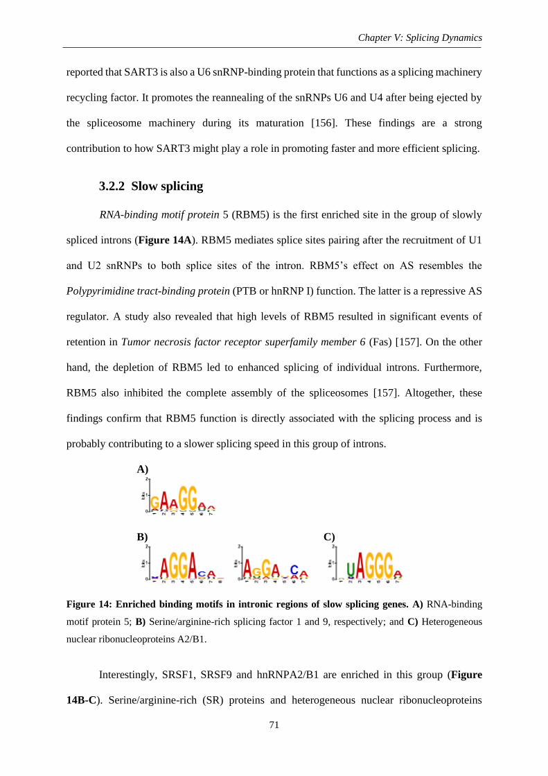
Figure 14: Enriched binding motifs in intronic regions of slow splicing genes ...................... 71

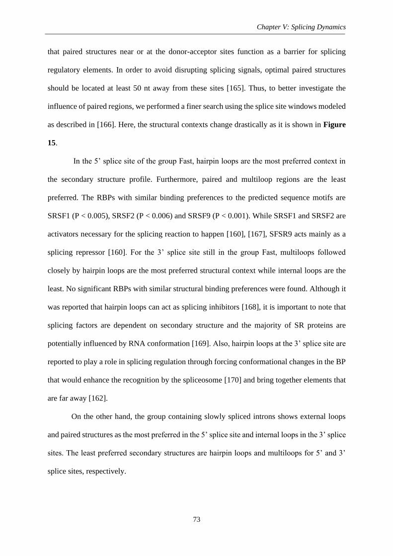
Figure 15: RNA secondary structure binging preferences ....................................................... 74

ix

List of Tables and Boxes


Box 1: Ribonucleic acid (RNA) ................................................................................................. 4

Table 1: Types of RNA .............................................................................................................. 6

Box 2: Spliceosome: A dynamic machinery ............................................................................ 10

Box 3: Chromatin immunoprecipitation .................................................................................. 17

Box 4: Real-time quantitative reverse transcription PCR (RT-qPCR) .................................... 19

Box 5: RNA sequencing (RNA-Seq) ....................................................................................... 21


Table 1: Datasets used in the present study ............................................................................. 28

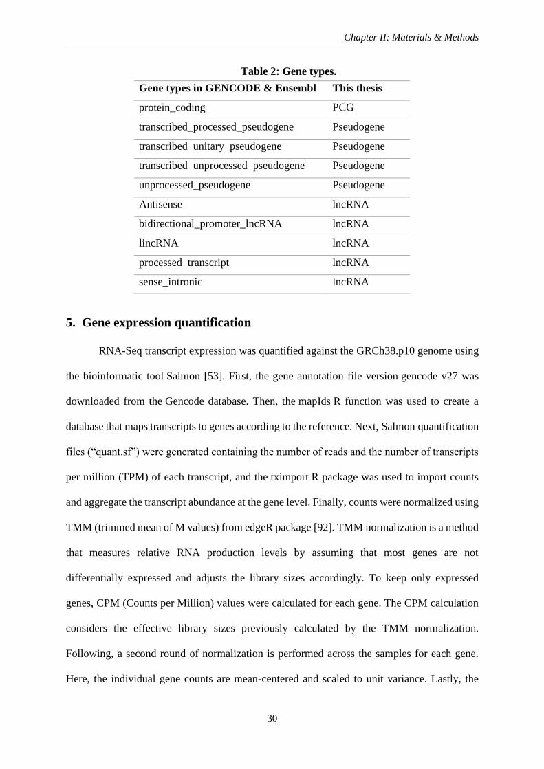
Table 2: Gene types ................................................................................................................. 30

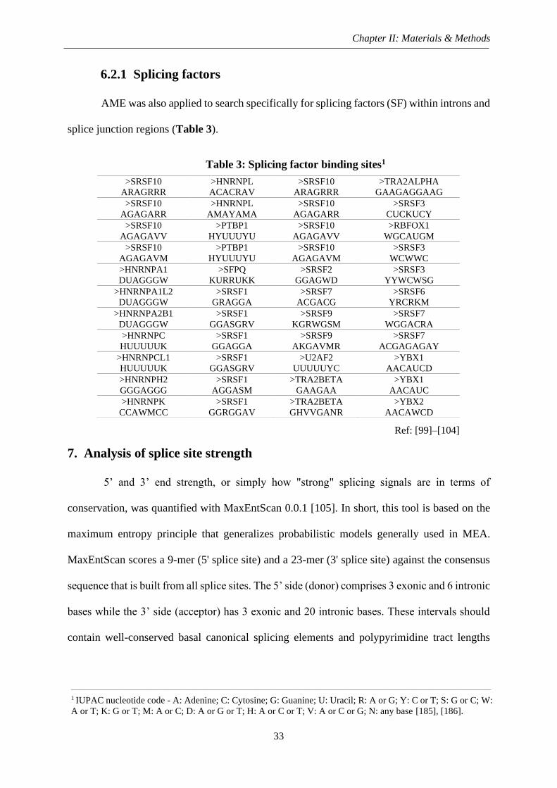
Table 3: Splicing factor binding sites ...................................................................................... 33

CHAPTER III: SPLICE-q .................................................................................................... 35

Table 1: Summary table of parameters .................................................................................... 43

CHAPTER IV: SPLICING DYNAMICS ............................................................................ 54

Table 1: Number of input reads per sample ............................................................................. 56

x

To my family

Thank you for everything!

À minha família

Obrigada por tudo!

∞

CHAPTER I.

Introduction

2

Chapter I: Introduction

Since the structure of DNA was discovered, the fields of cell and molecular biology

have been trying to decipher how the information contained in this molecule is read by the

cells. The biological instructions encoded by the DNA are carried by another nucleic acid, the

RNA, which is generated through a process called transcription. The RNA undergoes a series

of highly regulated post-transcriptional (or co-transcriptional) processing steps, including RNA

splicing. Important findings regarding RNA splicing have demonstrated how this process is

fundamental in the biology of the cell. Nevertheless, a vast field is yet to be explored

concerning the dynamics of transcript processing. This chapter will introduce basic concepts

of molecular biology focusing mainly on pre-mRNA splicing, its regulatory mechanisms, and

how its misregulation impacts the functionality of the cell. Then, sequencing technologies - in

particular, RNA sequencing - and its key applications will be described. Lastly, we show how

bioinformatics approaches can be applied to better understand splicing.

*

Chapter 1: Introduction

3

1. The eukaryotic gene

Deoxyribonucleic acid (DNA) is a linear polymer carrying chemical information in the

genetic code of all known cellular organisms and numerous viruses. The DNA is composed of

monomeric units called nucleotides, each consisting of a phosphate group, a deoxyribose and

a nitrogenous base. The DNA’s nitrogenous bases are the purines adenine and guanine, and the

pyrimidines thymine and cytosine [1]. For convenience, the bases are commonly abbreviated

as A, G, T, C, respectively. In 1953, Watson and Crick showed the purines binding to

pyrimidine bases through hydrogen bonds allowing the construction of a stable double-helix:

A preferentially binds to T via a double hydrogen bond while C binds to G via a triple bond

(A=T; G≡C) [2]. Furthermore, the nucleotides are linked together by phosphodiester bonds

established between the phosphate group and the C3 hydroxyl group of the adjacent nucleotide

[1]. The sequence of nucleotides, also known as genetic information, carried by the DNA,

encodes the instructions for growth, development, reproduction and more.

The term “gene” was first introduced in 1909 by Wilhelm Johannsen as a “unit of

heredity” and its definition has been changing over the years. In the 1960s, it was defined as a

continuous DNA sequence segment, encoding a polypeptide chain. Although it is still

employed today, this definition is outdated. Most recently, the molecular concept of gene was

redefined by Portin and Wilkins as [3]:

“…a DNA sequence (whose component segments do not necessarily

need to be physically contiguous) that specifies one or more

sequence-related RNAs/proteins that are both evoked by GRNs

[genetic regulatory networks] and participate as elements in

GRNs, often with indirect effects, or as outputs of GRNs, the latter

yielding more direct phenotypic effects.”

The eukaryotic gene is characterized by a series of exons, intercalated by sequences

with no coding potential called introns. During transcription, exons and introns are linearly


4

transcribed into a molecule of RNA (Box 1). Thereafter, the introns are excised in a process

known as splicing [4]. The number of introns per gene varies greatly within a genome and

when comparing genomes from different species. On average, a human gene has eight introns

of approximately 3.300bp in length, while the exons are much shorter (mean of 245bp) [5]. A

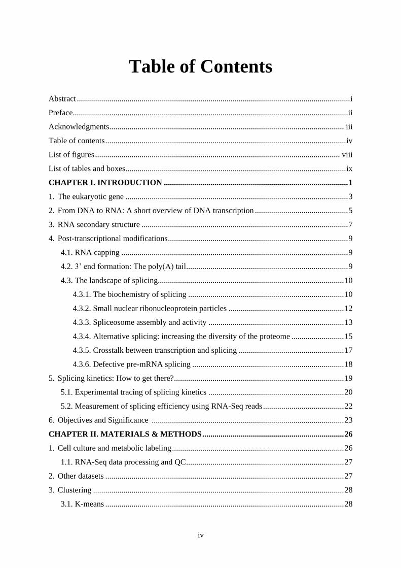
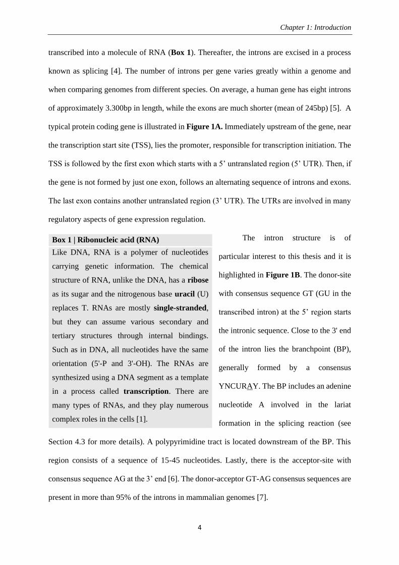
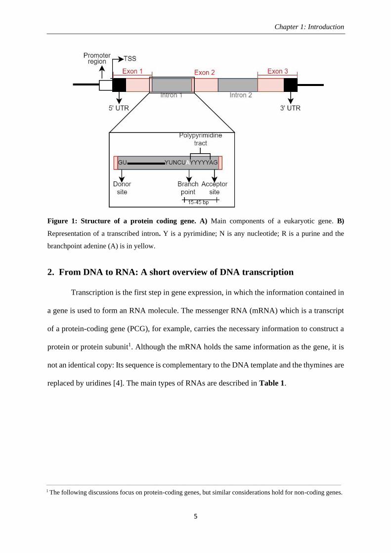
typical protein coding gene is illustrated in Figure 1A. Immediately upstream of the gene, near

the transcription start site (TSS), lies the promoter, responsible for transcription initiation. The

TSS is followed by the first exon which starts with a 5’ untranslated region (5’ UTR). Then, if

the gene is not formed by just one exon, follows an alternating sequence of introns and exons.

The last exon contains another untranslated region (3’ UTR). The UTRs are involved in many

regulatory aspects of gene expression regulation.

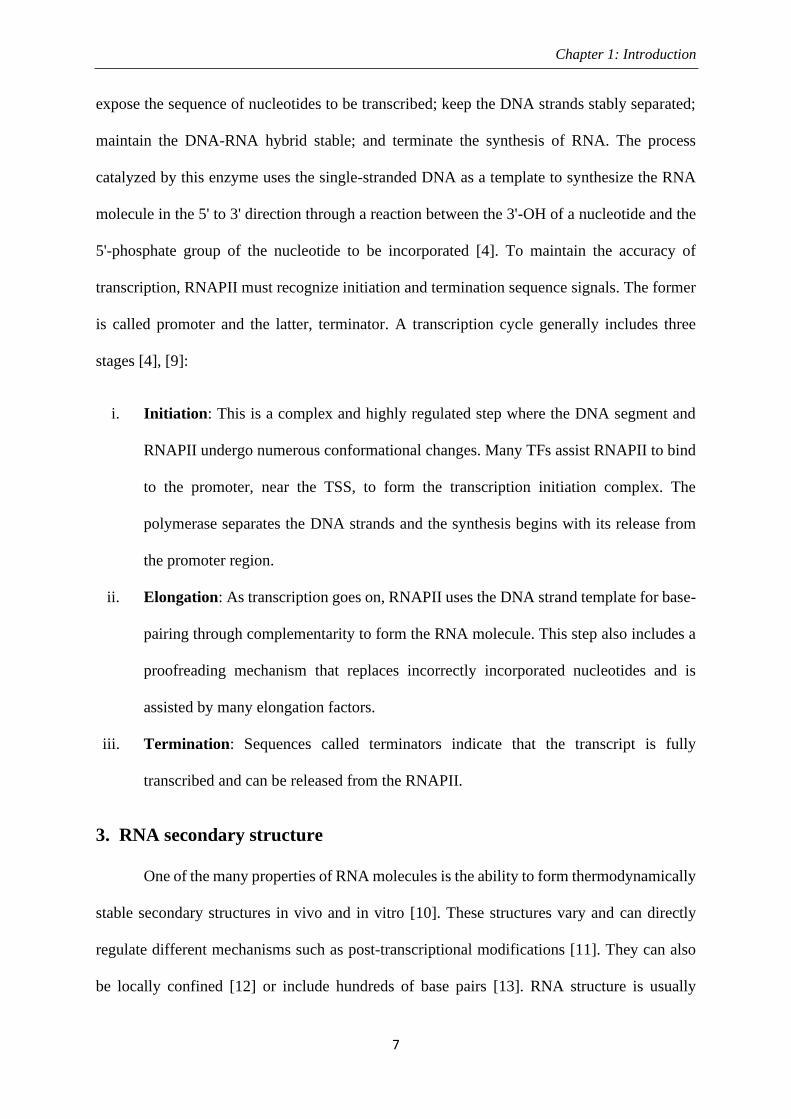
The intron structure is of

particular interest to this thesis and it is

highlighted in Figure 1B. The donor-site

with consensus sequence GT (GU in the

transcribed intron) at the 5’ region starts

the intronic sequence. Close to the 3' end

of the intron lies the branchpoint (BP),

generally formed by a consensus

YNCURAY. The BP includes an adenine

nucleotide A involved in the lariat

formation in the splicing reaction (see

Section 4.3 for more details). A polypyrimidine tract is located downstream of the BP. This

region consists of a sequence of 15-45 nucleotides. Lastly, there is the acceptor-site with

consensus sequence AG at the 3’ end [6]. The donor-acceptor GT-AG consensus sequences are

present in more than 95% of the introns in mammalian genomes [7].

Box 1 | Ribonucleic acid (RNA)

Like DNA, RNA is a polymer of nucleotides

carrying genetic information. The chemical

structure of RNA, unlike the DNA, has a ribose

as its sugar and the nitrogenous base uracil (U)

replaces T. RNAs are mostly single-stranded,

but they can assume various secondary and

tertiary structures through internal bindings.

Such as in DNA, all nucleotides have the same

orientation (5'-P and 3'-OH). The RNAs are

synthesized using a DNA segment as a template

in a process called transcription. There are

many types of RNAs, and they play numerous

complex roles in the cells [1].


5

Figure 1: Structure of a protein coding gene. A) Main components of a eukaryotic gene. B)

Representation of a transcribed intron. Y is a pyrimidine; N is any nucleotide; R is a purine and the

branchpoint adenine (A) is in yellow.

2. From DNA to RNA: A short overview of DNA transcription

Transcription is the first step in gene expression, in which the information contained in

a gene is used to form an RNA molecule. The messenger RNA (mRNA) which is a transcript

of a protein-coding gene (PCG), for example, carries the necessary information to construct a

protein or protein subunit1. Although the mRNA holds the same information as the gene, it is

not an identical copy: Its sequence is complementary to the DNA template and the thymines are

replaced by uridines [4]. The main types of RNAs are described in Table 1.

__________________________________________________________________________________________________________________________________________

1 The following discussions focus on protein-coding genes, but similar considerations hold for non-coding genes.


6

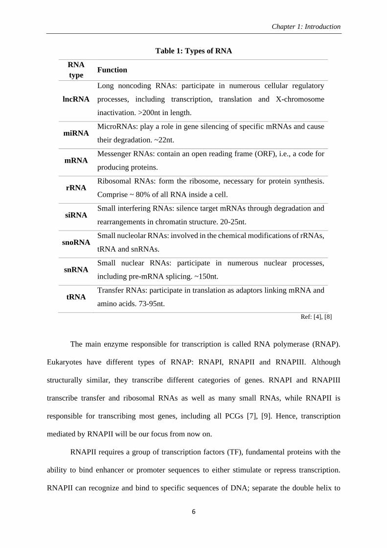
Table 1: Types of RNA

RNA

type Function

lncRNA

Long noncoding RNAs: participate in numerous cellular regulatory

processes, including transcription, translation and X-chromosome

inactivation. >200nt in length.

miRNA MicroRNAs: play a role in gene silencing of specific mRNAs and cause

their degradation. ~22nt.

mRNA Messenger RNAs: contain an open reading frame (ORF), i.e., a code for

producing proteins.

rRNA Ribosomal RNAs: form the ribosome, necessary for protein synthesis.

Comprise ~ 80% of all RNA inside a cell.

siRNA Small interfering RNAs: silence target mRNAs through degradation and

rearrangements in chromatin structure. 20-25nt.

snoRNA Small nucleolar RNAs: involved in the chemical modifications of rRNAs,

tRNA and snRNAs.

snRNA Small nuclear RNAs: participate in numerous nuclear processes,

including pre-mRNA splicing. ~150nt.

tRNA Transfer RNAs: participate in translation as adaptors linking mRNA and

amino acids. 73-95nt.

Ref: [4], [8]

The main enzyme responsible for transcription is called RNA polymerase (RNAP).

Eukaryotes have different types of RNAP: RNAPI, RNAPII and RNAPIII. Although

structurally similar, they transcribe different categories of genes. RNAPI and RNAPIII

transcribe transfer and ribosomal RNAs as well as many small RNAs, while RNAPII is

responsible for transcribing most genes, including all PCGs [7], [9]. Hence, transcription

mediated by RNAPII will be our focus from now on.

RNAPII requires a group of transcription factors (TF), fundamental proteins with the

ability to bind enhancer or promoter sequences to either stimulate or repress transcription.

RNAPII can recognize and bind to specific sequences of DNA; separate the double helix to


7

expose the sequence of nucleotides to be transcribed; keep the DNA strands stably separated;

maintain the DNA-RNA hybrid stable; and terminate the synthesis of RNA. The process

catalyzed by this enzyme uses the single-stranded DNA as a template to synthesize the RNA

molecule in the 5' to 3' direction through a reaction between the 3'-OH of a nucleotide and the

5'-phosphate group of the nucleotide to be incorporated [4]. To maintain the accuracy of

transcription, RNAPII must recognize initiation and termination sequence signals. The former

is called promoter and the latter, terminator. A transcription cycle generally includes three

stages [4], [9]:

i. Initiation: This is a complex and highly regulated step where the DNA segment and

RNAPII undergo numerous conformational changes. Many TFs assist RNAPII to bind

to the promoter, near the TSS, to form the transcription initiation complex. The

polymerase separates the DNA strands and the synthesis begins with its release from

the promoter region.

ii. Elongation: As transcription goes on, RNAPII uses the DNA strand template for base-

pairing through complementarity to form the RNA molecule. This step also includes a

proofreading mechanism that replaces incorrectly incorporated nucleotides and is

assisted by many elongation factors.

iii. Termination: Sequences called terminators indicate that the transcript is fully

transcribed and can be released from the RNAPII.

3. RNA secondary structure

One of the many properties of RNA molecules is the ability to form thermodynamically

stable secondary structures in vivo and in vitro [10]. These structures vary and can directly

regulate different mechanisms such as post-transcriptional modifications [11]. They can also

be locally confined [12] or include hundreds of base pairs [13]. RNA structure is usually


8

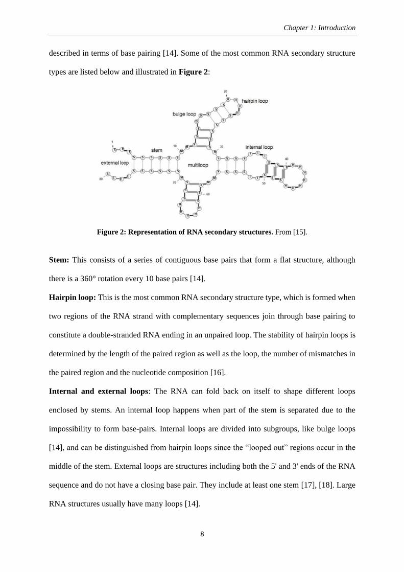
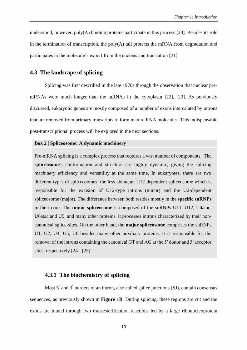
described in terms of base pairing [14]. Some of the most common RNA secondary structure

types are listed below and illustrated in Figure 2:

Figure 2: Representation of RNA secondary structures. From [15].

Stem: This consists of a series of contiguous base pairs that form a flat structure, although

there is a 360° rotation every 10 base pairs [14].

Hairpin loop: This is the most common RNA secondary structure type, which is formed when

two regions of the RNA strand with complementary sequences join through base pairing to

constitute a double-stranded RNA ending in an unpaired loop. The stability of hairpin loops is

determined by the length of the paired region as well as the loop, the number of mismatches in

the paired region and the nucleotide composition [16].

Internal and external loops: The RNA can fold back on itself to shape different loops

enclosed by stems. An internal loop happens when part of the stem is separated due to the

impossibility to form base-pairs. Internal loops are divided into subgroups, like bulge loops

[14], and can be distinguished from hairpin loops since the “looped out” regions occur in the

middle of the stem. External loops are structures including both the 5' and 3' ends of the RNA

sequence and do not have a closing base pair. They include at least one stem [17], [18]. Large

RNA structures usually have many loops [14].


9

Multiloop: these more complex structures are formed by hairpin loops that may be separated

by unpaired bases or not [14].

4. Post-transcriptional modifications

The recently synthesized RNAs, or primary RNAs, need to go through some processing

steps in order to produce mature RNA products. In this context, the precursor mRNA (pre-

mRNA) is a type of primary transcript which, after processing, becomes a messenger RNA

(mRNA). The main post-transcriptional modifications are 5' capping, 3’ polyadenylation and

splicing. On many occasions, they are tightly connected to transcription elongation and, for

this reason, are also known as co-transcriptional modifications. This section will be focusing

mostly on splicing.

4.1 RNA capping

The 5ʹ-methyl cap is the first modification of pre-mRNAs in eukaryotes and some

viruses. This 'cap' consists of modified guanine (m7G(5’)ppp(5’)X) and protects the new RNA

molecule as soon as it emerges from the RNAPII complex [19]. This modification aids the cell

in identifying different types of RNA. For instance, RNAPI and RNAPIII transcribe only

uncapped RNAs. The 5ʹ-methyl cap plays a role in the nuclear export of the RNA, protection

from exonuclease degradation, splicing and translation [4], [19].

4.2 3’-end formation: The poly(A) tail

As transcription is reaching its end, two important enzymes called cleavage stimulation

factor (CstF) and cleavage and polyadenylation specificity factor (CPSF) recognize specific

signals on the newly transcribed RNA for further processing. Once bound, other accessory

proteins form the 3' end of the emerging mRNA. Then, after the RNA is separated from the

RNAPII, the poly-A polymerase (PAP) acts by adding a tail of ~200 adenines at the recently

cut 3' end. The mechanism by which the total length of this poly(A) tail is defined is poorly


10

understood, however, poly(A) binding proteins participate in this process [20]. Besides its role

in the termination of transcription, the poly(A) tail protects the mRNA from degradation and

participates in the molecule’s export from the nucleus and translation [21].

4.3 The landscape of splicing

Splicing was first described in the late 1970s through the observation that nuclear pre-

mRNAs were much longer than the mRNAs in the cytoplasm [22], [23]. As previously

discussed, eukaryotic genes are mostly composed of a number of exons intercalated by introns

that are removed from primary transcripts to form mature RNA molecules. This indispensable

post-transcriptional process will be explored in the next sections.

4.3.1 The biochemistry of splicing

Most 5 ́ and 3 ́ borders of an intron, also called splice junctions (SJ), contain consensus

sequences, as previously shown in Figure 1B. During splicing, these regions are cut and the

exons are joined through two transesterification reactions led by a large ribonucleoprotein

Box 2 | Spliceosome: A dynamic machinery

Pre-mRNA splicing is a complex process that requires a vast number of components. The

spliceosome's conformation and structure are highly dynamic, giving the splicing

machinery efficiency and versatility at the same time. In eukaryotes, there are two

different types of spliceosomes: the less abundant U12-dependent spliceosome which is

responsible for the excision of U12-type introns (minor) and the U2-dependent

spliceosome (major). The difference between both resides mostly in the specific snRNPs

in their core. The minor spliceosome is composed of the snRNPs U11, U12, U4atac,

U6atac and U5, and many other proteins. It processes introns characterized by their non-

canonical splice-sites. On the other hand, the major spliceosome comprises the snRNPs

U1, U2, U4, U5, U6 besides many other auxiliary proteins. It is responsible for the

removal of the introns containing the canonical GT and AG at the 5′ donor and 3′ acceptor

sites, respectively [24], [25].


11

complex called spliceosome (Box 2) [26]. This well-described large ribonucleoprotein (RNP)

complex includes five small nuclear RNAs (snRNA), which together recognize the SJs and

the BP, forming the major spliceosome [27], [28].

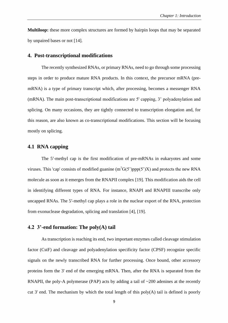
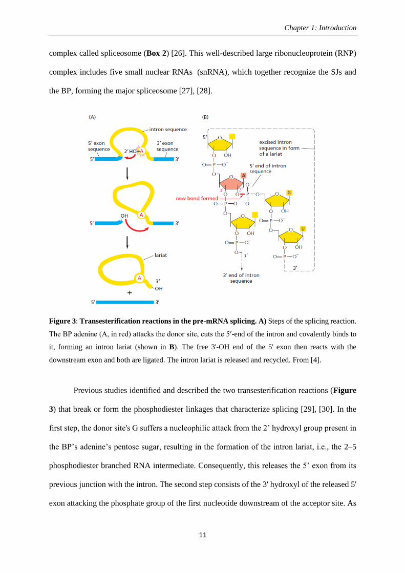
Figure 3: Transesterification reactions in the pre-mRNA splicing. A) Steps of the splicing reaction.

The BP adenine (A, in red) attacks the donor site, cuts the 5ʹ-end of the intron and covalently binds to

it, forming an intron lariat (shown in B). The free 3'-OH end of the 5' exon then reacts with the

downstream exon and both are ligated. The intron lariat is released and recycled. From [4].

Previous studies identified and described the two transesterification reactions (Figure

3) that break or form the phosphodiester linkages that characterize splicing [29], [30]. In the

first step, the donor site's G suffers a nucleophilic attack from the 2’ hydroxyl group present in

the BP’s adenine’s pentose sugar, resulting in the formation of the intron lariat, i.e., the 2–5

phosphodiester branched RNA intermediate. Consequently, this releases the 5’ exon from its

previous junction with the intron. The second step consists of the 3' hydroxyl of the released 5'

exon attacking the phosphate group of the first nucleotide downstream of the acceptor site. As


12

a result, the 5’ and now detached 3’ exon are joined, and the intron lariat is released, marking

the end of splicing. The spliceosome is also responsible for the folding of introns that facilitates

these reactions and for the precise recognition and pairing of the splice sites [24].

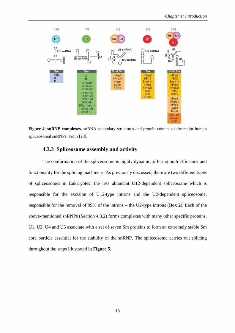
4.3.2 Small nuclear ribonucleoprotein particles

The small nuclear ribonucleoproteins (snRNPs) are essential components of the

spliceosome and mediate the catalysis of pre-mRNA splicing. These RNA-protein complexes

are formed from uridine-rich small nuclear RNA (non-coding RNA) and a wide collection of

proteins (Figure 4). snRNPs are classified into two groups: Sm snRNAs and Sm-like snRNAs

(Lsm). The former includes U1, U2, U4, U4atac, U5, U11 and U12 snRNAs, which present

three essential recognition parts: a 5′-trimethylguanosine cap, an Sm-protein-binding site and

a 3′ stem-loop structure. The second group is composed of U6 and U6atac snRNAs, containing

5'-γ-monomethyl phosphate cap and a 3' stem-loop [31].

After transcription, Sm-snRNAs are exported to the cytoplasm in a process facilitated

by an export machinery that subsequently disassociates from the pre-snRNA. Each snRNA

associates with a set of seven Sm proteins (B/B′, D1, D2, D3, E, F and G) to form an extremely

stable Sm core particle, essential for the stability of the snRNP. This step is carried out by the

survival motor neuron (SMN) protein complex. Initially, the SMN complex binds to conserved

regions in the snRNA. Then, the 5' cap is hypermethylated by trimethylguanosine synthase-1

and the 3'-end is trimmed by an exonuclease. These modifications are necessary for the

transport of the processed snRNP particle back into the nucleus where the Sm-class snRNPs

are targeted to Cajal bodies for the next maturation steps. Finally, the newly produced snRNPs

are stored in interchromatin granule clusters to be later used in pre-mRNA splicing [28], [31].


13

Figure 4: snRNP complexes. snRNA secondary structures and protein content of the major human

spliceosomal snRNPs. From [28].

4.3.3 Spliceosome assembly and activity

The conformation of the spliceosome is highly dynamic, offering both efficiency and

functionality for the splicing machinery. As previously discussed, there are two different types

of spliceosomes in Eukaryotes: the less abundant U12-dependent spliceosome which is

responsible for the excision of U12-type introns and the U2-dependent spliceosome,

responsible for the removal of 99% of the introns – the U2-type introns (Box 2). Each of the

above-mentioned snRNPs (Section 4.3.2) forms complexes with many other specific proteins.

U1, U2, U4 and U5 associate with a set of seven Sm proteins to form an extremely stable Sm

core particle essential for the stability of the snRNP. The spliceosome carries out splicing

throughout the steps illustrated in Figure 5.


14

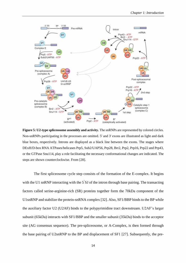
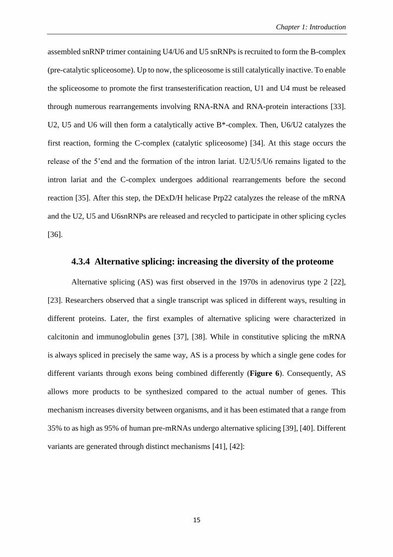
Figure 5: U2-type spliceosome assembly and activity. The snRNPs are represented by colored circles.

Non-snRNPs participating in the processes are omitted. 5' and 3' exons are illustrated as light and dark

blue boxes, respectively. Introns are displayed as a black line between the exons. The stages where

DExH/D-box RNA ATPases/helicases Prp5, Sub2/UAP56, Prp28, Brr2, Prp2, Prp16, Prp22 and Prp43,

or the GTPase Snu114, play a role facilitating the necessary conformational changes are indicated. The

steps are shown counterclockwise. From [28].

The first spliceosome cycle step consists of the formation of the E-complex. It begins

with the U1 snRNP interacting with the 5 ́SJ of the intron through base pairing. The transacting

factors called serine-arginine-rich (SR) proteins together form the 70kDa component of the

U1snRNP and stabilize the protein-snRNA complex [32]. Also, SF1/BBP binds to the BP while

the auxiliary factor U2 (U2AF) binds to the polypyrimidine tract downstream. U2AF’s larger

subunit (65kDa) interacts with SF1/BBP and the smaller subunit (35kDa) binds to the acceptor

site (AG consensus sequence). The pre-spliceosome, or A-Complex, is then formed through

the base pairing of U2snRNP to the BP and displacement of SF1 [27]. Subsequently, the pre-


15

assembled snRNP trimer containing U4/U6 and U5 snRNPs is recruited to form the B-complex

(pre-catalytic spliceosome). Up to now, the spliceosome is still catalytically inactive. To enable

the spliceosome to promote the first transesterification reaction, U1 and U4 must be released

through numerous rearrangements involving RNA-RNA and RNA-protein interactions [33].

U2, U5 and U6 will then form a catalytically active B*-complex. Then, U6/U2 catalyzes the

first reaction, forming the C-complex (catalytic spliceosome) [34]. At this stage occurs the

release of the 5’end and the formation of the intron lariat. U2/U5/U6 remains ligated to the

intron lariat and the C-complex undergoes additional rearrangements before the second

reaction [35]. After this step, the DExD/H helicase Prp22 catalyzes the release of the mRNA

and the U2, U5 and U6snRNPs are released and recycled to participate in other splicing cycles

[36].

4.3.4 Alternative splicing: increasing the diversity of the proteome

Alternative splicing (AS) was first observed in the 1970s in adenovirus type 2 [22],

[23]. Researchers observed that a single transcript was spliced in different ways, resulting in

different proteins. Later, the first examples of alternative splicing were characterized in

calcitonin and immunoglobulin genes [37], [38]. While in constitutive splicing the mRNA

is always spliced in precisely the same way, AS is a process by which a single gene codes for

different variants through exons being combined differently (Figure 6). Consequently, AS

allows more products to be synthesized compared to the actual number of genes. This

mechanism increases diversity between organisms, and it has been estimated that a range from

35% to as high as 95% of human pre-mRNAs undergo alternative splicing [39], [40]. Different

variants are generated through distinct mechanisms [41], [42]:


16

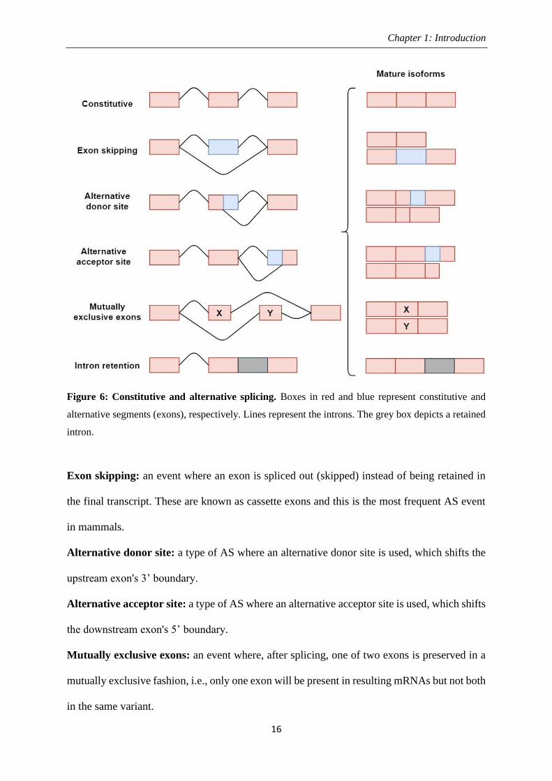
Figure 6: Constitutive and alternative splicing. Boxes in red and blue represent constitutive and

alternative segments (exons), respectively. Lines represent the introns. The grey box depicts a retained

intron.

Exon skipping: an event where an exon is spliced out (skipped) instead of being retained in

the final transcript. These are known as cassette exons and this is the most frequent AS event

in mammals.

Alternative donor site: a type of AS where an alternative donor site is used, which shifts the

upstream exon's 3’ boundary.

Alternative acceptor site: a type of AS where an alternative acceptor site is used, which shifts

the downstream exon's 5’ boundary.

Mutually exclusive exons: an event where, after splicing, one of two exons is preserved in a

mutually exclusive fashion, i.e., only one exon will be present in resulting mRNAs but not both

in the same variant.


17

Intron retention: the least prevalent of the AS types in mammals, consists of the retention of

an intronic sequence. The retained intron may then become part of the coding region which

will often cause the production of a non-functional protein. A recent study showed how intron

retention is connected to transcription and acts widely in the regulation of gene expression [43].

4.3.5 Crosstalk between transcription and splicing

Splicing is dynamic and occurs mostly during or immediately after the transcription of

a complete intron. Co-transcriptional splicing was first suggested in D. melanogaster chorion

genes using electron microscopy to observe the assembly of spliceosomes at the splice

junctions in nascent transcripts [45]. Further, studies applying ChIP (chromatin

immunoprecipitation, Box 3) revealed that the steps of the spliceosome assembly are similar

to the way it is assembled in vitro in yeast and mammals, increasing evidence for the co-

transcriptional nature of splicing [46],

[47]. In addition to these findings, further

studies investigated introns that are co-

transcriptionally spliced. More recently,

genome-wide studies in different cell

lines and organisms using nascent RNA

showed introns being spliced shortly after

their transcription is finished: in S.

cerevisiae, data revealed polymerase

pausing at the terminal exon, permitting

enough time for splicing to happen before

the release of the mature RNA [48]; and analysis of nascent RNA also indicated that most

introns in D. melanogaster are co-transcriptionally spliced [49], as well as in mouse [50] and

many human cells and tissues [51]–[53]. Several other studies showed how splicing also

Box 3 | Chromatin immunoprecipitation

Chromatin immunoprecipitation, or simply

ChIP, is an experimental approach commonly

used to investigate the biological significance of

DNA-protein interactions inside the cell.

Through ChIP, DNA and the protein of interest

are cross-linked and then the complexes are

immunoprecipitated using antibodies that target

the protein. Subsequently, the cross-link is

reversed followed by purification of the ChIP-

enriched DNA. The DNA sequences associated

with the precipitated protein can be further

identified by other molecular biology techniques

such as polymerase chain reaction (PCR) [44].


18

interferes with transcription through different mechanisms involving, for example, SR proteins

[54] and effects on chromatin [55], [56]. For further information, Oesterreich and colleagues

have written an interesting and detailed review on co-transcriptional splicing [57].

4.3.6 Defective pre-mRNA splicing

Since the overwhelming majority of human genes include introns, and up to 95% of

human pre-mRNAs undergo AS, it is natural to think that disturbances of regular splicing may

have negative consequences. Over 20 years ago, it was estimated that up to 15% of mutations

that cause genetic disease affect pre-mRNA splicing [58]. However, this number is probably

an underestimation as it only considers mutations in classical splice-site sequences. Indeed,

mutations in other splicing regulatory sites can result in multiple outcomes, namely exon

skipping, mutation-associated intron retention and introduction of pseudo-splice-sites. The last

two events, in most cases, cause premature termination codons1 to be introduced, consequently

resulting in degradation and loss of function [59].

Naturally, since efficient pre-mRNA splicing is essential, its misregulation is related to

numerous human diseases. For instance, Duchenne muscular dystrophy can be caused by a

mutation in the DMD gene, which leads to the deficiency of the protein dystrophin. Therapies

targeting the deleterious effects of these mutations through the modulation of dystrophin

splicing were shown to be promising [60]. Furthermore, aberrant splicing in glioblastoma, an

aggressive brain tumor, promotes the survival and proliferation of the cancerous cells. However,

splicing-redirecting approaches and regulation of splicing factors could positively interfere

with tumor development [61].

A lot of progress has been made towards the understanding of how splicing affects

diseases and cancer biology together with an effort to understand how “splicing correction”

approaches could be beneficial for therapy [60], [62], [63]. Yet, to better understand the

dynamics of splicing and the perturbations that might be caused by aberrant transcript


19

processing, it is important to quantify splicing efficiency. These aspects will be discussed in

the following sections.

5. Splicing kinetics: how to get there?

Understanding the splicing kinetics, i.e., how splicing events are coordinated and

quantified is essential. The efficiency of splicing is commonly quantified by means of RT-

qPCR (Box 4) with primers that span exon-exon and exon-intron boundaries [65]. A strong

signal obtained from the first is indicative that

an intron has already been excised. On the

other hand, strong signals from the later

indicate transcripts from which the intron has

not yet been spliced out. Yet, this

methodology can only investigate a limited

number of genes. By contrast, transcriptomics

technologies, such as RNA-Seq, allow these

analyses from a genome-wide point of view.

Below, these technologies are summarized.

Although every cell in an organism

contains the same genome, different cells and

tissues will show a different expression

profile. The transcriptome is the set and amount of RNA present in a cell, tissue or even an

organism and represents its physiological state. Studying the transcriptome allows scientists to

get a deeper understanding of the functional elements of the genome as well as its role in

development, health and disease. Through high-throughput transcriptomics it is possible to

Box 4 | Real-time quantitative reverse

transcription PCR (RT-qPCR)

RT-qPCR is a sensitive and powerful

experimental approach for quantifying

genetic material through the production of

copies of a target sequence or genetic

fragment. It involves the combination of

cDNA reverse transcription and the

amplification of the DNA targets through

PCR to detect and measure, for example, the

amount of specific RNA. This is possible

since the amplification step is followed by

the use of fluorescence [64]. RT-qPCR may

be used in different ways such as the

quantification of gene expression,

transcription and splicing kinetics, and in

clinical settings.

__________________________________________________________________________________________________________________________________________

1 A codon is a nucleotide triplet which encodes for an amino acid, except for a termination or stop codon which

act as termination sites, indicating the end of the protein-coding sequence [4].


20

identify most - if not all – mRNAs, non-coding RNAs and small RNAs; investigate gene

structures, e.g. TSS, 5’ and 3’ ends, the number of exons and introns, splicing patterns; and

quantify expression levels [66]. Over the years, different technologies for analyzing the

transcriptome have been developed. When it comes to quantifying splicing efficiency, RNA

Sequencing (RNA-Seq) stands out. This technology is described in more detail in Box 5.

5.1 Experimental tracing of splicing kinetics

From the splicing efficiency perspective, RNA-Seq allows us, for example, to assess

nascent transcripts before introns have been totally spliced out—i. e., within short intervals of

time after the transcription has started [67]. Experimentally, this can be achieved through

metabolic labeling with uridine (U) analogs such as 4-thiouridine (4sU), 5-etyniluridine (EU)

and 5′-bromo-uridine (BrU) over a time course [68]. Shortly, this method consists of exposing

the RNAPII to one of these labeled compounds (pulse step) that is used in the synthesis of new

RNA transcripts for a short, well-defined period. Next, the unlabeled substance (here, normal

uridine) is added (chase step) and the production of RNA continues, but without the labeled

compound from the pulse phase. Lastly, the labeled RNAs are isolated and prepared for

sequencing [69], [70]. This type of assay is also called pulse-chase analysis and it can provide

information concerning RNA transcription and the primary transcript processing that occurred

during the chosen labeling period. In addition, incorporating the chase step in time points

allows the investigation of the fate of the nascent RNA over time as well as its processing [71].

Barrass and colleagues [72], for example, took advantage of this approach to investigate

the kinetics of RNA processing. Focusing specially on splicing, and using labeling times as

short as 1.5 minutes, they studied short-lived non-coding RNAs as well as intron-containing

pre-mRNAs in Saccharomyces cerevisiae. Through metabolic labeling, they were able to

assess nascent transcription and revealed the significant association between non-coding RNA


21

Box 5 | RNA Sequencing (RNA-Seq)

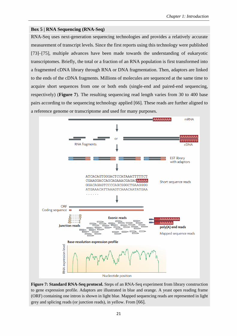
RNA-Seq uses next-generation sequencing technologies and provides a relatively accurate

measurement of transcript levels. Since the first reports using this technology were published

[73]–[75], multiple advances have been made towards the understanding of eukaryotic

transcriptomes. Briefly, the total or a fraction of an RNA population is first transformed into

a fragmented cDNA library through RNA or DNA fragmentation. Then, adaptors are linked

to the ends of the cDNA fragments. Millions of molecules are sequenced at the same time to

acquire short sequences from one or both ends (single-end and paired-end sequencing,

respectively) (Figure 7). The resulting sequencing read length varies from 30 to 400 base

pairs according to the sequencing technology applied [66]. These reads are further aligned to

a reference genome or transcriptome and used for many purposes.

Figure 7: Standard RNA-Seq protocol. Steps of an RNA-Seq experiment from library construction

to gene expression profile. Adaptors are illustrated in blue and orange. A yeast open reading frame

(ORF) containing one intron is shown in light blue. Mapped sequencing reads are represented in light

grey and splicing reads (or junction reads), in yellow. From [66].


22

length, secondary structures and stability – findings that would not have been possible in wild-

type cells at steady state.

Another way to assess nascent transcripts is through the purification of chromatin-

associated nascent RNAs. In this approach, the cells are biochemically fractionated before

RNA isolation, enabling the analysis of the different steps in the lifetime of RNA molecules

[76].

5.2 Measurement of splicing efficiency using RNA-Seq reads

For intron-containing transcripts, splicing efficiency can be determined with different

frameworks that use read counts on intronic and exonic regions. In other words, an RNA-Seq

experiment can function as a "snapshot" of the RNA while splicing is still ongoing with the

splicing efficiency being the fraction of molecules that have already been spliced. Short-read

RNA-Seq is currently the main approach using either nascent or total RNA.

Conceptually, splicing efficiency can be observed either from an intron-centric point of

view—to investigate whether an intron has been spliced out—or from an exon-centric point of

view—to investigate whether an exon has been correctly spliced within the context of its

transcript.

Khodor et al. [49] used an intron-centric method to estimate the unspliced fraction of

introns in D. melanogaster by taking the ratio of the read coverage of the last 25 bp of an intron

and the first 25 bp of the following exon. In this way, introns, where the RNA polymerase has

not yet reached the acceptor splice site, are not included but the metric is not guaranteed to take

values between 0 and 1 and does hence not constitute an efficiency metric in the strict sense.

Tilgner et al. [52] used deep-sequencing of human subcellular fractions and developed an exon-

centric “completed splicing index” (coSI) which takes reads spanning the 5’ and the 3’ splice

junctions of an exon and computes the fraction of reads indicating completed splicing, i.e.,

which span from exon to exon, to study co-transcriptional splicing. By explicitly considering


23

also reads which span from the upstream exon directly to the downstream exon, this approach

includes exon skipping events, but coSI values for the first and last exon of a transcript cannot

be determined. More recently, Převorovský et al. [77] presented a workflow for genome-wide

determination of intron-centric splicing efficiency in yeast. The efficiencies are quantified for

the 5’ and 3’ splice junctions separately as the number of “transreads” (split reads spanning

from exon to exon) divided by the number of reads covering the first or last base of the intron,

respectively. Although the authors call their metric “splicing efficiency”, it is not limited to a

range from 0 to 1 and it is not clear how cases without intronic reads (divisions by zero) are

handled. Other drawbacks of this workflow are that it consists of numerous open-source tools

and custom shell and R scripts and that it was explicitly developed for yeast.

6. Objectives and Significance

Although the above-mentioned frameworks for calculating splicing efficiency from

RNA-Seq data exist, there is more to add to their respective limitations. The bioinformatics

steps involved might be challenging - including difficulties in running workflows that require

long running times and the installation of numerous tools - specially for experimental

biologists. Thus, we present here a user-friendly open-source Python tool for genome-wide

quantification of splicing efficiencies.

The objectives of the present work include: (i) Implement a complete and user-friendly

tool for genome-wide quantification of splicing efficiencies from RNA-Seq data. (ii) Provide

an in-depth study that addresses different temporal splicing patterns and their underlying

biological features using time-course nascent RNA-Seq data. These features include gene and

intron length, gene and intron nucleotide composition (GC content), gene expression levels,

gene biotype, gene function and intron ordinal position. Search for common motifs at splice

junctions to look for relevant regulatory elements influencing the splicing dynamics. Also,

analyze the RNA secondary structure elements and their RBP binding preferences.


24

Focus on splicing efficiency measurement using the newest and the most efficient

methods is important for understanding the impact of its regulation. It is also a contribution to

a global understanding of many biological processes in multiple organisms, including

mechanisms behind numerous human diseases. This project will certainly align with

bioinformatics and RNA biology needs and will be helpful to future research in these fields.

*

25

CHAPTER II.

Materials & Methods

Chapter II: Materials & Methods

26

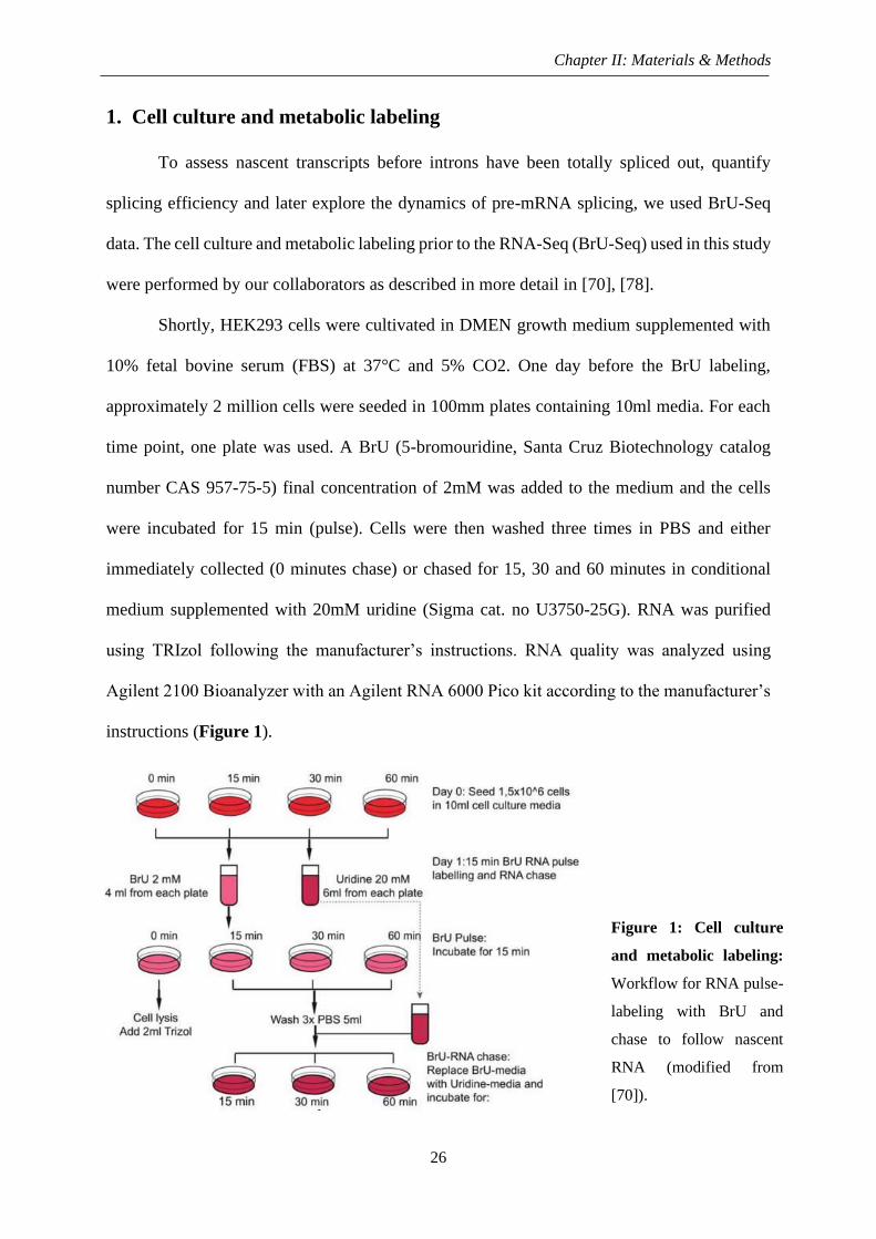
1. Cell culture and metabolic labeling

To assess nascent transcripts before introns have been totally spliced out, quantify

splicing efficiency and later explore the dynamics of pre-mRNA splicing, we used BrU-Seq

data. The cell culture and metabolic labeling prior to the RNA-Seq (BrU-Seq) used in this study

were performed by our collaborators as described in more detail in [70], [78].

Shortly, HEK293 cells were cultivated in DMEN growth medium supplemented with

10% fetal bovine serum (FBS) at 37°C and 5% CO2. One day before the BrU labeling,

approximately 2 million cells were seeded in 100mm plates containing 10ml media. For each

time point, one plate was used. A BrU (5-bromouridine, Santa Cruz Biotechnology catalog

number CAS 957-75-5) final concentration of 2mM was added to the medium and the cells

were incubated for 15 min (pulse). Cells were then washed three times in PBS and either

immediately collected (0 minutes chase) or chased for 15, 30 and 60 minutes in conditional

medium supplemented with 20mM uridine (Sigma cat. no U3750-25G). RNA was purified

using TRIzol following the manufacturer’s instructions. RNA quality was analyzed using

Agilent 2100 Bioanalyzer with an Agilent RNA 6000 Pico kit according to the manufacturer’s

instructions (Figure 1).

Figure 1: Cell culture

and metabolic labeling:

Workflow for RNA pulse-

labeling with BrU and

chase to follow nascent

RNA (modified from

[70]).


27

1.1 RNA-Seq data processing and QC

The library was prepared with TrueSeq Stranded Total RNA Kit (Illumina). Sequencing

was performed on Illumina HiSeq 2500 to obtain an average of ~200 million read pairs per

sample. The strand-specific reads were mapped to GRCh38.p10 with STAR v2.7.1a [79]

according to recommendations from the STAR manual 2.4.0.1. The index was built on gencode

v27 (ftp://ftp.ebi.ac.uk/pub/databases/gencode/Gencode_human/release27/gencode.v27.anno

tation.gtf.gz). The GEO [80] accession numbers for these sequencings are GEO: GSE92565

and GSE83561.

FastQC [81] was used for quality control on the raw sequence data. This tool provides

a simple and quick quality control (QC) summary on raw sequencing data, imported as BAM,

SAM or Fastq files. The results are shown as modular graphs and tables that track data issues

that should be addressed before further analysis. The modules of FastQC include basic statistics

such as read counts and length, sequence quality and content, GC content bias, read length

distribution, duplication levels, overrepresented sequences and adapter and k-mer content.

Each issue should be addressed with caution while taking into consideration the context of

what is expected from the library. For the present samples and type of sequencing, there were

no problematic issues.

DeepTools2.0 [82] was used to assess genome-wide similarity of the sequencing

replicates. This is computed by correlating the read coverages in consecutive bins of 10

kilobases in all samples. Replicates are highly correlated with an average ρ = 0.95 which fits

the ENCODE consortium recommendations for biological replicates [83].

2. Other datasets

The other datasets processed and analyzed in this thesis are described in Table 1.


28

Table 1: Datasets used in the present study.

Accession/

Reference

Genome/

Annotation Description

GSE84722

[84]

GRCh38.p10/

gencode v27

HEK293 cells labeled with uridine analog 4-tU for 0

(total), 7.5, 15, 30, 45, and 60 minutes and collected

in triplicate. Sequenced on HiSeq2500.

GSE70378

[85] Ensembl R64-1-1

S. cerevisiae labeled with 4tU labeling for 1.5, 2.5

and 5 minutes. Total RNA-Seq was also performed.

All experiments were performed in triplicate.

Sequenced on HiSeq2500.

GSE133626

[86]

GRCh38.p10/

gencode v27

Total RNA from fresh frozen prostate cancer tissue

along with a matched normal control sample. Patient

15 of the dataset. Sequenced in duplicate on

HiSeq2000.

GSE30567

[52]

GRCh38.p10/

gencode v27

HNEK cell compartments data Poly(A) and

nonPoly(A) selected. Sequenced on Illumina

Genome Analyzer II.

3. Clustering

As part of the analysis performed in the second part of this thesis (Chapter IV), we used

splicing efficiency values quantified from the BrU-seq data (described at the beginning of this

chapter) to group introns.

3.1 K-means

K-means clustering was computed with R function kmeans with k = 70 and nstart =

100. K-means [87] is an unsupervised learning algorithm, i.e., the algorithm cannot predict

results and simply tries to find trends in the data. The number of clusters must be determined

beforehand. Each observation is randomly allocated to a cluster, and the centroid of each cluster

is determined. The algorithm iterates through the following steps [88]:


29

i. Assign each observation to the clusters (k).

ii. Identify the centroid (mean point) of each cluster.

iii. Compute the distances of the centroids from each data point and place it into the cluster

with the minimum distance from the centroid.

iv. Compute the centroid of the new cluster found and repeat the steps until the minimum

within-cluster variation is reached. This variation is computed as the least squared

Euclidean distance between each point and the centroid of the cluster it belongs to.

3.2 Hierarchical clustering

To get the previously generated clusters into groups assigned according to intron

splicing dynamics (fast, intermediate and slow), Agglomerative Hierarchical Clustering (AHC)

was computed using the centroids of the 70 clusters. In short, AHC assigns each observation

to a cluster, then the distance between each cluster is computed and the two closest clusters are

merged. The steps are repeated until there is only one cluster, i.e., the clusters can be formed

following a hierarchy - from bottom to top or vice-versa [88].

The R function agnes was chosen due to the agglomerative coefficient (AC) it provides.

This value varies from 0 to 1 and measures the cluster structure, thus allowing for the best

method to be chosen. An AC closer to 1 suggests a strong cluster structure. Ward’s method

was chosen, and the resulting cluster was represented as a dendrogram. Ward's method aims at

reducing the overall within-cluster variance by merging clusters with minimum between-

cluster distances at each step combined with minimum information loss [88], [89].

4. Gene type annotation

Gene types from the genes present in this study were retrieved from BiomaRt [90], [91].

The Protein Coding Gene (PCG), Pseudogene and Long Non-coding RNA (lncRNA)

categories were defined as described in Table 2.


30

Table 2: Gene types.

5. Gene expression quantification

RNA-Seq transcript expression was quantified against the GRCh38.p10 genome using

the bioinformatic tool Salmon [53]. First, the gene annotation file version gencode v27 was

downloaded from the Gencode database. Then, the mapIds R function was used to create a

database that maps transcripts to genes according to the reference. Next, Salmon quantification

files (“quant.sf”) were generated containing the number of reads and the number of transcripts

per million (TPM) of each transcript, and the tximport R package was used to import counts

and aggregate the transcript abundance at the gene level. Finally, counts were normalized using

TMM (trimmed mean of M values) from edgeR package [92]. TMM normalization is a method

that measures relative RNA production levels by assuming that most genes are not

differentially expressed and adjusts the library sizes accordingly. To keep only expressed

genes, CPM (Counts per Million) values were calculated for each gene. The CPM calculation

considers the effective library sizes previously calculated by the TMM normalization.

Following, a second round of normalization is performed across the samples for each gene.

Here, the individual gene counts are mean-centered and scaled to unit variance. Lastly, the

Gene types in GENCODE & Ensembl This thesis

protein_coding PCG

transcribed_processed_pseudogene Pseudogene

transcribed_unitary_pseudogene Pseudogene

transcribed_unprocessed_pseudogene Pseudogene

unprocessed_pseudogene Pseudogene

Antisense lncRNA

bidirectional_promoter_lncRNA lncRNA

lincRNA lncRNA

processed_transcript lncRNA

sense_intronic lncRNA


31

counts were voom transformed (limma package [93]). Shortly, Voom is an approach that

robustly and non-parametrically estimates the mean-variance relaionhsip of the log-counts

normalized for sequence depth (log-cpm). Then, as a function of average log-count, the mean-

variance trend is incorporated into a precision weight for each normalized observation

individually [94].

6. Motif enrichment analysis (MEA)

6.1 Transcription start sites (TSS)

To evaluate how transcription factors and other DNA binding proteins influence the

splicing dynamics, we first applied HOMER’s (Hypergeometric Optimization of Motif

EnRichment) [95] findMotifs.pl which analyzes promoter sequences and searches for motifs

that are enriched in the target sequences relative to others (background). The input is a list of

gene identifiers such as Ensembl gene ID, Entrez gene ID, Refseq, etc. Ensembl gene IDs were

provided, and motifs of length 8 to 20 nucleotides were searched from -400 to +100 relative to

each gene’s TSS. The HOMER differential motif discovery algorithm applies zero or one

occurrence per sequence scoring (ZOOPS) together with hypergeometric enrichment

calculations (or binomial) to define motif enrichment significance. findMotifs.pl operates

according to the following steps:

i. Converts the gene accession numbers provided as input to a consistent gene identifier

(Entrez gene ID).

ii. Selects a meaningful background.

iii. Performs Gene Ontology (GO) enrichment quantification of various categories of gene

function, biological pathways, domain structure, chromosome location, etc. The GO

enrichment assumes a hypergeometric distribution.

iv. Assigns weights to background sequences according to the CpG distribution in the

targets in a way that comparable numbers of low and high-CpG sequences are analyzed.


32

v. Performs de novo motif analysis. HOMER searches for motifs that are over-represented

in the target sequences (input) relative to the background using the cumulative

hypergeometric distribution (or cumulative binomial distribution for large data sets).

Motifs are first found by exhaustively checking for simple motif enrichment and later

refining the best candidates into accurate probability matrices.

vi. Generates an HTML output for the de novo analysis containing non-redundant motifs

sorted by p-value.

vii. Performs motif enrichment analysis of known motifs and generated the HTML output

file. The "known motifs" are derived from published ChIP-seq data.

6.2 RNA-binding proteins (RBPs)

The MEME suite’s v5.1.1 [96] Analysis of Motif Enrichment (AME) program [97],

was used with default parameters to identify known enriched RPB motifs. AME uses a

parameter-free linear regression method to identify biological patterns within the nucleotide

sequences. In other words, the user is not required to select a threshold on the biological signal

for partitioning the genes into negative or positive sets. The groups of introns defined as Fast

and Slow splicing generated through clustering (section 3 of this chapter) were used as control

and background of one another. The input should contain sequences in FASTA format which

we extracted using getfasta from Bedtools 2.27.0 [98]. AME detects known motifs provided

by the user which are comparatively enriched in the input sequences compared to control

sequences. For this, we chose the RNA-binding motifs available at [99]. Furthermore, AME

scores a series of sequences with a motif, treating each sequence as a possible match for the

pattern. Numerous types of sequence scoring functions are supported, and the motif

occurrences are handled equally, i.e., regardless of their locations in the sequence . We used

the average odds score (default) in which the average PWM (position weight matrix) motif

score of the sequence is used. The statistical test used for testing motif enrichment was one-

tailed Fisher's exact test. The output is an HTML file containing only significantly enriched

motifs.


33

6.2.1 Splicing factors

AME was also applied to search specifically for splicing factors (SF) within introns and

splice junction regions (Table 3).

Table 3: Splicing factor binding sites1

Ref: [99]–[104]

7. Analysis of splice site strength

5’ and 3’ end strength, or simply how "strong" splicing signals are in terms of

conservation, was quantified with MaxEntScan 0.0.1 [105]. In short, this tool is based on the

maximum entropy principle that generalizes probabilistic models generally used in MEA.

MaxEntScan scores a 9-mer (5' splice site) and a 23-mer (3' splice site) against the consensus

sequence that is built from all splice sites. The 5’ side (donor) comprises 3 exonic and 6 intronic

bases while the 3’ side (acceptor) has 3 exonic and 20 intronic bases. These intervals should

contain well-conserved basal canonical splicing elements and polypyrimidine tract lengths

>SRSF10

ARAGRRR

>HNRNPL

ACACRAV

>SRSF10

ARAGRRR

>TRA2ALPHA

GAAGAGGAAG

>SRSF10

AGAGARR

>HNRNPL

AMAYAMA

>SRSF10

AGAGARR

>SRSF3

CUCKUCY

>SRSF10

AGAGAVV

>PTBP1

HYUUUYU

>SRSF10

AGAGAVV

>RBFOX1

WGCAUGM

>SRSF10

AGAGAVM

>PTBP1

HYUUUYU

>SRSF10

AGAGAVM

>SRSF3

WCWWC

>HNRNPA1

DUAGGGW

>SFPQ

KURRUKK

>SRSF2

GGAGWD

>SRSF3

YYWCWSG

>HNRNPA1L2

DUAGGGW

>SRSF1

GRAGGA

>SRSF7

ACGACG

>SRSF6

YRCRKM

>HNRNPA2B1

DUAGGGW

>SRSF1

GGASGRV

>SRSF9

KGRWGSM

>SRSF7

WGGACRA

>HNRNPC

HUUUUUK

>SRSF1

GGAGGA

>SRSF9

AKGAVMR

>SRSF7

ACGAGAGAY

>HNRNPCL1

HUUUUUK

>SRSF1

GGASGRV

>U2AF2

UUUUUYC

>YBX1

AACAUCD

>HNRNPH2

GGGAGGG

>SRSF1

AGGASM

>TRA2BETA

GAAGAA

>YBX1

AACAUC

>HNRNPK

CCAWMCC

>SRSF1

GGRGGAV

>TRA2BETA

GHVVGANR

>YBX2

AACAWCD

__________________________________________________________________________________________________________________________________________

1 IUPAC nucleotide code - A: Adenine; C: Cytosine; G: Guanine; U: Uracil; R: A or G; Y: C or T; S: G or C; W:

A or T; K: G or T; M: A or C; D: A or G or T; H: A or C or T; V: A or C or G; N: any base [185], [186].


34

upstream of the 3' splice site, respectively. A high score should mean a high similarity between

the input and the consensus sequence, i.e., a “strong” splice site.

8. RBP preferences for secondary structure

Knowing that RBPs recognize both sequence and structure aspects in their binding sites,

RBPmotif [106] was applied to predict sequence (de novo motif search) and stable secondary

structure binding preferences of RBPs in a 100bp window around the splice junctions –

allowing us to investigate if RNA secondary structure preferences differ according to the speed

of splicing. The secondary structure prediction uses RNAplfold. This algorithm computes local

pair probabilities for base pairs. Briefly, this algorithm considers the collection of all potential

RNA sequence structures to quantify probabilities in various structural contexts for each base.

The type of secondary structure representation chosen was PHIME which has different

structural contexts: paired (P), hairpin loop (H), internal loop (I), multiloop (M), external loop

(E). These structures are described in more detail in Chapter I. A “secondary structure profile”

matrix is computed, and each entry represents the probability of a base to be present in a given

structural context. Parameters of the secondary structure are weighted so that the most desired

context is equal to 1. A web service is available at rnamotif.org.

*

35

CHAPTER III.

Results: SPLICE-q

Chapter III: SPLICE-q

36

Results: SPLICE-q

We have previously described the frameworks available to quantify splicing efficiency

from RNA-Seq data. However, the bioinformatics steps involved to reach the quantifications

might be challenging, specially for experimental biologists as they would include numerous

tool installations and long running times. Aiming to overcome these challenges, this chapter

will introduce the approach used to develop SPLICE-q, an up-to-date and user-friendly tool for

SPLICing Efficiency quantification.

*


37

1. SPLICE-q

SPLICE-q is a tool implemented in Python 3 for quantification of individual intron

splicing efficiency from strand-specific RNA-Seq data. SPLICE-q's main quantification

method uses splicing reads – both split and unsplit – spanning the splice junctions of a given

intron (Figure 1). Split reads are junction reads spanning from one exon to another, thus

indicating processed transcripts from which the individual intron has already been excised.

Intuitively, unsplit reads are those spanning the intron-exon boundaries (covering both sides of

the splice junction), hence, indicating transcripts from which the intron has not yet been spliced

out. As an alternative measure for splicing efficiency, SPLICE-q computes an inverse intron

expression ratio (IER), which compares the introns’ expression levels with those of their

flanking exons.

Figure 1: Read assignment scheme for splicing efficiency (SE) and inverse intron expression ratio

(IER). Illustration of the reads used by SPLICE-q to quantify SE and IER. In yellow, split reads at the

5’ splice junction; in orange, split reads at the 3’ splice junction; in green, unsplit reads at the 5’ splice

junction; in dark blue, unsplit reads at the 3’ splice junction. In gray and blue, the areas covering the

exons and introns, respectively. In white, reads not overlapping splice junctions.

1.1 Quantifying splicing efficiency and inverse intron expression ratio

Splicing efficiency (SE): SPLICE-q uses split and unsplit junction reads to quantify SE

for each intron individually. It determines the RNA-Seq reads mapping to both splice junctions

of an intron, distinguishes split and unsplit reads for the 5’ and 3’ splice junctions of this intron


38

and estimates a splicing efficiency score (SEi) as a function of the corresponding read counts

as follows:

𝑆𝐸𝑖 =∑ Si

jj∈{5′,3′}

∑ (Sij+Ni

j)j∈{5′,3′}

0 ≤ 𝑆𝐸𝑖 ≤ 1 (Eq.1)

Where S and N are the numbers of split and unsplit reads, respectively, which map to the 5’-

end (5′) and 3’-end (3′) splice junction of a given intron i.

An SE of 0 indicates that the intron has not been spliced out in any of the transcripts

from which the junction reads originate, which may be due to late splicing in the case of nascent

RNA-Seq or intron retention in the case of steady-state RNA-Seq. An SE of 1 means completed

splicing on all transcripts. Therefore, SE values ranging between 0 and 1 approximate the

fraction of molecules that have already been spliced. This quantification method makes it

possible to compare spliced and unspliced intron rates directly.

Inverse intron expression ratio (IER): as an alternative measure for splicing

efficiency when using Level 3 filtering, SPLICE-q also provides the inverse of the ratio of

intron expression to exon expression, where Ix is the median per-base read coverage of the x-

th intron of a given transcript and Ex and Ex+1 represent the corresponding median coverages

of the flanking exons:

𝐼𝐸𝑅 = 1 −min (1,Ix

0.5∙(Ex+Ex+1)) 0 ≤ 𝐼𝐸𝑅 ≤ 1 (Eq.2)

Here, the focus lies specifically on the per-base median coverage of all reads mapping

to the involved genomic elements (exonic and intronic reads) rather than just the splice

junctions (Figure 1). As explained above, a high SE indicates that an intron was spliced out of

a large fraction of transcripts. This scenario should display high read coverage in the exons and


39

low coverage or none in the intron. In other words, peaks of mapped reads are observed in the

surrounding exons when compared to the intron itself. On the contrary, introns with a low SE

should have read coverage profiles more similar to the surrounding exons.

1.2 Workflow and parameters

SPLICE-q is also sensitive to the overlap of genomic elements. In other words,

SPLICE-q takes into consideration when a genome shows overlapping features that can cause

issues with a correct assignment of reads to specific introns or exons. For example, for intron-

exon boundaries overlapping exons of other genes, seemingly unsplit reads might instead stem

from exonic regions of the overlapping genes. This is problematic due to the RNA-Seq

methodology’s limitation that makes it difficult to confidently determine without ambiguity to

which genomic element, exon or intron, these reads should be attributed [107].

Therefore, SPLICE-q allows the user to select different levels of restrictiveness for

strand-specific filtering, including (i) Level 1: keep all introns in the genome regardless of

overlaps with other genomic elements; (ii) Level 2: select only introns whose splice junctions

do not overlap any exon in different genes; (iii) Level 3: select only introns that do not overlap

with any exon of the same or different genes (Figure 2). The two necessary input files are:

i. A Binary Alignment Map (BAM) file, which is simply the binary version of a Sequence

Aligned Map (SAM) file. Sequence alignment tools, such as STAR [79], provide BAM

files as output and, in other cases, the conversion from SAM to BAM can be easily achieved

with Samtools [108].

ii. A genome annotation file provided by GENCODE [109] or Ensembl [110] in Gene

Transfer Format (GTF) containing information on exons and the genes and transcripts they

are associated with.


40

Figure 2: SPLICE-q’s levels of restrictiveness. (Level 1) keep all introns in the genome regardless of

overlaps with other genomic elements; (Level 2) select only introns whose splice junctions do not

overlap any exon in different genes; (Level 3) select only introns that do not overlap with any exon of

the same or different genes. A and A.1 are isoforms of the same gene (A) and B represents a different

gene.

SPLICE-q’s internal default workflow comprises of the following major steps (Figure 3):

i. Parsing of genomic features from the GTF file;

ii. Locating and annotating introns and splice junctions from the GTF’s exon coordinates;

iii. Filtering of introns according to the level of restrictiveness based on the overlap of

genomic elements;

iv. The selection of split and unsplit reads at the splice junctions according to the reads’

concise idiosyncratic gapped alignment report (CIGAR), and subsequent coverage

calculation for each individual splice junction.

v. Computation of splicing efficiencies (SE).

For Level 3 filtering, when the user chooses to include the inverse intron expression ratio, the

workflow includes the following steps (Figure 4):

i. Parsing of genomic features from the GTF;

ii. Locating and annotating exons, introns and splice junctions.

iii. Filtering of introns that do not overlap with any exon of the same or different genes;

iv. Computation of median per-base coverages of introns and their flanking exons

v. Computation of the inverse intron expression ratios (IER).


41

Figure 3: SPLICE-q’s default workflow. Dashed lines indicated steps that depend on parameter

settings. Solid lines represent the mandatory steps of the workflow. A BAM index (.bai) file is generated

if not provided by the user (yellow). Arrows in blue represent a lookup in the data structure they pass

through. SJ = splice junction; TSV = tab-separated vector.


42

Figure 4: SPLICE-q’s inverse intron expression ratio workflow. Dashed lines indicate steps

where parameters can be set up. Solid lines represent the mandatory steps of the workflow. The

generation of an index (.bai) file is mandatory if not provided by the user (yellow). Arrows in blue

represent a lookup in the data structure they pass through. I = Introns, E = Exons, SJ = splice junctions.

The standard output is a 14-column tab-separated values (TSV) file containing:

chromosome, strand, ensemble gene stable ID, ensemble transcript stable ID, intron number,

SJ5’ start position, SJ5’ end position, SJ5’ split read count, SJ5’ unsplit read count, SJ3’ start

position, SJ3’ end position, SJ3’ split read count, SJ3’ unsplit read count, SE score. When


43

running with the inverse intron expression ratio option, the program outputs a 15-column TSV

consisting of chromosome, strand, ensemble gene stable ID, ensemble transcript stable ID,

intron number, intron start position, intron end position, 5’ exon median coverage, SJ5’ split

read count, SJ5’ unsplit read count, intron median coverage, SJ3’ split read count, SJ3’ unsplit

read count, SE score and IER. SPLICE-q’s default will only count reads with unique alignment,

but the user can choose whether to include reads aligned to multiple places in the genome

according to mapping quality scores. Other filters can also be set up according to users’

requirements (Table 1).

Table 1: Summary table of parameters.

Parameter Description

MinCoverage Minimum number of reads spanning each splice junction (Default =

10).

MinReadQuality Mapping quality. By default, only uniquely mapped reads are included

(Default = 10).

MinIntronLength Minimum intron length. Default value is optimal for analysis using

human RNA-Seq data (Default = 30) [111].

FilterLevel

(1) keep all introns in the genome regardless of overlaps with other

genomic elements.

(2) select only introns whose SJs do not overlap any exon in different

genes

(3) select only introns that do not overlap with any exon of the same

or different gene (Default).

EIRatio Running mode that additionally outputs exonic and intronic coverage

ratio. Restricted by FilterLevel.

NProcesses

Multiple concurrent processes are used to minimize running times and

the number of processes can be adjusted by the user through this

parameter. Generates an index (.bai) file.


44

1.3 Compatibility and requirements

SPLICE-q requires pysam (https://github.com/pysam-developers/pysam) and uses

modified functions from GTFtools [112]. The efficient data structure for working with

intervals and checking for genomic overlaps is provided by the InterLap module

(https://github.com/brentp/interlap). Due to pysam’s requirements, SPLICE-q is limited to

macOS and Linux platforms but can be run on Windows 10 through its subsystem for Linux.

1.4 Fast and user-friendly quantification of splicing efficiency

SPLICE-q’s run time with default parameters for approximately 100 million input reads

mapped to the human genome is 18 minutes using a MacBook Pro with a Dual-Core Intel Core

i5 processor and 8GB of RAM. By increasing the number of processes to 4 or 8, which is not

an issue considering nowadays’ number of processor cores of most laptops and desktops, the

running time on an AMD Opteron 6282 SE with 516GB of memory is less than 2 minutes

(Figure 5a). Memory usage is low, being approximately that of the GTF file size (1.4 GB for

the human genome; Figure 5b). SPLICE-q’s approach provides major advantages over

previous workflows which may require the installation of numerous tools and suffer from long

running times.


45

Figure 5: SPLICE-q’s run time and memory usage. a) Run time for approximately 100 million input

reads mapped to the human genome. b) Memory usage for 1.4GB GTF. Time in seconds.

*

a) Time (in minutes)

0

5

10

15

20

25

p 1 p 4 p 8

Level 1

Level 2

Level 3

b)

46

CHAPTER IV.

Results: SPLICE-q Application

Chapter IV: Splicing Kinetics

Chapter IV: SPLICE-q Application

47

Results: SPLICE-q Application

In Chapter III, we introduced the approach used to develop SPLICE-q, a tool for

SPLICing Efficiency quantification. Understanding the splicing kinetics, i.e., how splicing

events are coordinated and quantified is essential. Thus, in this Chapter, we show the usefulness

of SPLICE-q by applying it to various datasets including two different species and different

methodologies.

*


48

1. Splicing kinetics in human and yeast

We applied SPLICE-q to globally assess the kinetics of intron excision. The goal here

is to show the tool’s applicability using different data. For this purpose, we performed three

different analyses using data from two species and different methodologies (Chapter II, Table

1). The first set of sequencing data is a strand-specific paired-end nascent and total RNA-Seq

of human embryonic kidney cells (HEK293). Cells were progressively labeled with 4SU for

7.5, 15, 30, 45 and 60 minutes before the RNA was purified (nascent RNA) [84]. There was an

average number of ~31 million uniquely mapped read pairs per sample. SPLICE-q was applied

with default parameters: filtering level 3, minimum coverage of 10 uniquely mapped reads at

each splice junction and minimum intron length of 30 nucleotides. Only introns satisfying the

filtering criteria in all samples after running SPLICE-q were kept, totaling ~10k introns. As

expected, SPLICE-q detects a progressive increase of SE throughout the time course (Figure

1a). Interestingly, at 7 Minutes, the SE scores are already high with a median of 0.65. This

agrees with previous studies showing that splicing is predominantly co-transcriptional in

humans and for the most part happens immediately after the transcription of an intron is

completed, when the RNA polymerase has proceeded only a few bases into the downstream

exon [45], [48], [51]–[53]. However, this value remains almost unchanged until the next time

point (Figure 1a), when it starts to increase again, gradually approaching the level at steady

state (total RNA): medians of 0.85 and 0.96 for the 60 minutes and total RNA sample,

respectively.

We chose a second dataset [85] which would allow us to quantify the splicing efficiency

of nascent RNA within a finer time scale. These sequencing experiments were performed with

4-thiouracil labeled RNA (4tU-seq) from Saccharomyces cerevisiae. Nascent RNA was

labeled for an extremely short time (1.5, 2.5 and 5 Minutes) and then sequenced [85] (Figure

1b). Unlabeled control samples were also generated. After alignment of the raw data, we


49

obtained an average of over 50 million uniquely mapped reads per sample and 246 introns –

from the

Figure 1: Splicing kinetics using different datasets. a) Time-series nascent and total RNA-Seq of

HEK293 cells; b) Time-series nascent and total RNA-Seq of S. cerevisiae; and c) RNA-Seq of human

subcellular fractions in K562 cells.

a)

b)

c)


50

total of 296 introns present in yeast [113] – shared between all samples after running SPLICE-

q with the above-mentioned default parameters and filtering level 2. The SE at 1.5 minutes has

a median of 0.29 while, strikingly, there is an increase of 131% in just one minute, with a

median SE of 0.67 at 2.5 minutes. This value does not alter in the next time point and the

unlabeled control sample shows a median SE of 0.93. This brief analysis suggests how essential

it is to perform short labeling in S. cerevisiae in order to assess its splicing kinetics since some

transcripts approximate steady-state levels in a time as short as 2.5 minutes.

The next dataset consists of deep sequencing of subcellular RNA fractions in human

immortalized myelogenous leukemia cells K562 [52]. The data include poly(A)- and poly(A)+

chromatin-associated total RNA and nuclear RNA, and cytosolic RNA. This approach allowed

SPLICE-q to assess the SE scores of introns in different levels of RNA processing in the cell

(Figure 1c). There was an average number of over 78 million uniquely mapped read pairs in

Poly(A)+ samples and over 54 million in the poly(A)-. As expected, most introns’ splicing is

fully completed in the cytosolic fraction. However, it is interesting to note that the Poly(A)-

samples have lower SE in all fractions when compared to their Poly(A)+ counterparts

(Wilcoxon's test, P ≤ 0.0001). The poly(A)- nuclear fraction has the lowest SE, while Cell

Poly(A)+ shows the highest. The high SE in the former suggests that splicing is happening

shortly after transcription is completed. Assessing the kinetics of pre-mRNA splicing in

subcellular fractions with SPLICE-q provides valuable information concerning the co-

transcriptionality of this process and allows the interrogation of the fraction of introns which

are post-transcriptionally spliced.

2. Analysis of prostate cancer data

Lastly, we show how SPLICE-q can also be applied to quantify intron retention in total

RNA-Seq data. For this purpose, we used data coming from a prostate cancer sample along

with its matched normal tissue (patient 15 of ref. [86]). Since for each of the tissues two


51

replicates were available, we computed splicing efficiencies for each replicate and then

averaged the results for the tumor tissue and the normal tissue.

Prostate cancer is one of the most common cancer types in men [114]. SPLICE-q

detected relatively high splicing efficiencies—median SE of 0.96 in both the tumor and the

normal sample—in the 66,389 introns shared across the sample pair after running the tool with

default parameters. This is expected when the tool is applied to steady-state RNA-Seq data.

Although this overview suggests that there is no alteration in average splicing efficiency levels

between normal and tumor tissue, a closer look showed interesting changes for individual

introns. One intriguing example is Prostate cancer associated 3 (PCA3), a long noncoding

RNA highly expressed in prostate cancer and widely known as a prostate-specific biomarker

of high specificity [115]. It has been found to be involved in the proliferation and survival of

prostate cancer cells by multiple mechanisms, including the modulation of androgen receptor

signaling, the inhibition of the tumor suppressor PRUNE2, and possibly by acting as a

competing endogenous RNA (ceRNA) for high mobility group box 1 (HMGB1) protein via

sponging of miR-218-5p [115]–[117]. Interestingly, PCA3’s second intron located at

chr9:76,782,833-76,783,704 has an SE of 0.57 in normal tissue and a much higher SE of 0.90

in the tumor (Figure 2a), suggesting that PCA3 might not only be overexpressed but also more

efficiently spliced.

Variation in splicing efficiency can be also observed among protein coding genes. The

retinoic acid-related orphan receptor β (RORβ, encoded by the gene RORB) was recently

reported to inhibit tumorigenesis in colorectal cancer in vivo. When RORβ was overexpressed,

the tumorigenic capacity of the cells was significantly reduced, suggesting that this protein acts

as a tumor suppressor in colorectal cancer [118]. In agreement with these previous findings,

we found two of the RORB introns—located at chr9:74,630,368-74,634,630 and


52

chr9:74,634,773-74,642,413—having reduced splicing efficiencies in the tumor sample (SEs

of 0.99 and 0.98

Figure 2: Processing dynamics profile of introns in prostate cancer and normal samples. IGV

views of representative cases of introns from different genes comparing prostate cancer vs. normal

samples. a) Intron located at chr9:76,782,833-76,783,704 from PCA3; b) Introns located at

chr9:74,630,368-74,634,630 and chr9:74,634,773-74,642,413 from RORB; and c) Intron located at

chrX:100,662,368-100,664,773 from SRPX2. Tumor and normal samples are represented in red and

blue, respectively.

in the normal control and 0.63 and 0.60 in the tumor, respectively) (Figure 2b). Contrasting,

Sushi repeat-containing protein X‐linked 2, or simply SRPX2, shows the opposite splicing

efficiency profile with an intron at the coordinates chrX:100,662,368-100,664,773 being less

efficiently spliced in the control sample (SE of 0.59) than in the tumor (SE of 0.90, Figure 2c).

Previous studies showed SRPX2 playing an important role in cancer development and

progression. In colorectal cancer, the overexpression of SRPX2 may promote the

invasiveness of tumor cells [119], and in prostate cancer, a knockdown of SRPX2 affected the

proliferation, migration and invasion of cancer cells by partially suppressing the

PI3K/Akt/mTOR signaling pathway [120]. PI3K/Akt/mTOR regulates cell proliferation and


53

survival in different cancer types and is usually activated in advanced prostate cancer [121],

[122]. Furthermore, the suppression of this signaling pathway was reported to reduce cell

motility and invasion in prostate cancer [123]. These examples illustrate that gene regulation

may go beyond the mere expression levels, with a gain or loss of splicing efficiency potentially

acting as a superposed mechanism that may be beneficial to tumor development.

*

54

CHAPTER V.

Results: Splicing Dynamics

Chapter V: Splicing Dynamics

55

Chapter IV: Splicing Dynamics

In the previous chapters, we showed that splicing efficiency can be determined with

certain molecular biology approaches or different frameworks including challenging

bioinformatics steps. We introduced SPLICE-q, a tool that makes it possible to quantify

splicing efficiency in a fast and precise way. But what is the relationship between splicing

efficiency and the biology of the cell? What biological aspects could be influencing splicing

kinetics? To answer these and many other questions, SPLICE-q was applied to globally assess

the kinetics of intron excision. This chapter aims to provide an in-depth study to address

questions concerning the differences in the speed of splicing and the underlying biological

features that might be associated with it using time-course nascent RNA-Seq data. Those

features include gene and intron length, gene and intron nucleotide composition (GC content),

gene biotype, gene function and intron ordinal position. We also searched for motifs at splice

junctions to look for relevant regulatory elements influencing the splicing dynamics. Lastly,

we analyzed the RNA secondary structure elements and its RBP binding preferences as well

as features associated with exons and UTRs.

*


56

1. Dataset and clustering step

To monitor splicing kinetics in human cells, we used RNA-Seq data from Human

Embryonic Kidney 293 cells (HEK293) after labeling with the uridine analog BrU (BrU-seq).

Shortly, the cells were incubated with 2mM of 5-bromouridine (BrU) and either collected

immediately (0 Minutes) or chased for 15, 30 and 60 minutes prior to RNA purification. The

data was mapped to the human genome (hg38) (see Chapter II). On average, we obtained 103

million read pairs per sample and approximately 85% of those were uniquely mapped (Table

1). These samples were compared to an unlabeled control with an average of 30 million paired-

end reads per replicate. Visual inspection of the mapped reads showed reads covering exonic

and intronic regions in the BrU-Seq while the unlabeled control covered mostly exons.

Table 1: Number of input reads per sample.

Input Reads

Time-point

(in minutes) Sample A

% Uniquely

mapped reads Sample B*

% Uniquely

mapped reads

0 107.855.496 83.78% 102.270.732 84.60%

15 113.149.174 86.74% 94.402.826 83.61%

30 103.679.161 89.48% 101.572.030 85.20%

60 93.184.721 83.59% 110.250.800 84.61%

*Sample B comprises 2 technical replicates.

SPLICE-q was applied using default parameters to quantify the splicing efficiency of

all samples. The table of results for each sample in each time point was merged in order to

keep only satisfying the filtering criteria in both samples at the same time. This totals 23.475,

23.767, 21.532, 37.067 and 60.762 introns in 0, 15, 30 and 60 minutes and control,

respectively. On the side of exploring the features shared by these introns according to their

splicing efficiency, only those shared between in all samples at the same time were taken. This

consists of 14.003 introns distributed in 3848 genes which satisfied SPLICE-q’s default


57

filtering criteria (Figure 1a). As expected, SPLICE-q detects a progressive increase of splicing

efficiency throughout the time course (Figure 1b). Samples were compared to total RNA to

assess the steady-state levels of splicing.

Figure 1: Splicing kinetics using BrU labeled RNA-Seq. a) Venn diagram showing the introns shared

between all samples of the BrU-Seq dataset. b) Splicing efficiency throughout the time course.

Only the 6024 introns whose SE has an absolute difference ≤ 0.2 between the two

replicates for all the time points of the time series were considered for downstream analyses

(Figure 2a). Two rounds of clustering were performed on individual introns using the average

(per replicate) SE scores in each time-point. First, K-means clustering was computed with

a)

b)


58

k = 70 (nstart = 100). Then, the centroids of each cluster were hierarchically clustered (Figure

2a). Introns with SE in a given time-point diverging in 0.2 or more from the centroid of their

cluster and clusters showing SEx+1 - SEx ≤ -0.2, with x indicating a time-point, were excluded.

To further investigate the kinetics of intron excision and the possibly associated underlying

biological features, three introns groups with distinct splicing efficiency were drawn from the

second round of clustering after final filtering: (i) Fast: introns with SE(0Min) ≥ 0.75, i.e.,

introns with high level of co-transcriptional splicing; (ii) Intermediate: introns with 0.3 <

SE(0Min) < 0.75 and SE(60Min) ≥ 0.75 ; and (iii) Slow: introns with SE(0Min) ≤ 0.3 and none

of the efficiencies in the other time-points exceeding 0.4 (Figure 2b). These groups were then

used to address questions concerning their splicing dynamics, i.e., the underlying biological

features that might be associated with the differences in the speed of splicing.

Figure 2: Workflow for intron clustering. a) Representation of how the groups were extracted,

guided by the results of the hierarchical clustering displayed as a dendrogram; and b) Average curve

representing the three groups according to their SE patterns through the time course: Fast, Intermediate

and Slow splicing speed.

0

0.2

0.4

0.6

0.8

1

0 Minutes 15 Minutes 30 Minutes 60 Minutes

SE

Fast Intermediate Slow

a)

b)


59

2. Biological features

2.1 Gene architecture

2.1.1 Length and nucleotide composition

Genes and genomes are highly heterogeneous concerning their length and nucleotide

composition. Previous studies showed how specially GC content has great variation in different

genomic regions and species [124]–[126]. In higher eukaryotes’ genomes, sequences of high

GC content are very common [127]. However, how nucleotide composition influences different

patterns of splicing speed has yet to be explored.

In the light of our data, we see a modest but significant increase of GC content in introns

and genes of the Slow splicing group when compared to Intermediate and Fast (Figure 3A-D,

P < 0.01, Wilcoxon rank test). This information alone is not enough to draw conclusions on

how GC content might contribute to splicing kinetics. Thus, knowing that GC-rich genes are

usually associated with smaller introns [128], we investigated whether our data would follow

this trend. In agreement with literature, introns belonging to the Slow splicing group are

significantly shorter than introns in groups Fast and Intermediate (P ≤ 0.05, Wilcoxon rank

test). Not surprisingly, gene length follows the same trend, since introns are much longer than

exons in the human genome [111]. Although the same study showed a strong negative

correlation between intron length and GC content [128], this phenomenon cannot be observed

in our data.

It is widely known that the range of functional elements in introns interact with features

of the exons [129]–[131]. Therefore, we checked for GC content and the length of exons

flanking introns in each group (Figure 4). In all groups, the flanking exons are significantly

GC-richer than the introns (P ≤ 0.01, Wilcoxon rank test). Previous studies showed this trend

and also suggested that this difference might be linked to more efficient transcription and

splicing [130], [132]. Additionally, exons in the Slow splicing group show significantly higher


60

exonic GC content when compared to the Fast group (P ≤ 0.01, Wilcoxon rank test). A possible

explanation for what could be influencing the higher GC content in the Slow splicing group is

the assortment of gene types present in this group.

Figure 3: Gene and intron nucleotide composition and length. A) GC content of the introns; B) GC

content of the complete genes; C) Length of the introns; and D) Length of the genes – defined as the

number of nucleotides before splicing in the primary transcript [133].

Figure 4: Nucleotide composition of exons. GC content of introns and flanking exons in each group.


61

We confirmed this by checking the protein coding genes (PCG), Pseudogenes and

lncRNA content in each group and, surprisingly, the Slow group is the one containing more

non-coding genes: 25% against ~1% only in the other two groups and when compared to all

the genes from this study (Figure 5). Furthermore, in the Slow splicing group, the exons from

the PCG have significantly lower GC content than the exons in the lncRNAs (P ≤ 0.01,

Wilcoxon rank test). The differences in GC content between introns and exons were suggested

to be one of the factors strongly influencing elements linked to transcription and splicing, such

as histone marks and nucleosome occupancy [129]. Furthermore, an increased GC content,

including in lncRNAs, might be linked to GC-rich RNA secondary structures. We will discuss

secondary structures later in this chapter. Exon length does not differ between groups (data not

shown).

Figure 5: Gene type. Distribution of gene biotypes in each group. Total = All genes from the 6024

introns analyzed in this thesis.

2.1.2 Intron ordinal position

We hypothesized that in each group the introns closer to the TSS would have different

characteristics when compared to other introns and when comparing groups. Our idea is

0.00

0.10

0.20

0.30

0.40

0.50

0.60

0.70

0.80

0.90

1.00

Fast Intermediate Slow Total

lncRNA

Pseudogene

PCG

Gene type


62

partially supported by literature, e.g., Chen and colleagues, in a study limited to only two

chromosomes, observed that the first introns are usually longer than the downstream introns

[134]. In agreement with literature, we see that the first introns in the Fast group are

significantly longer than the other introns in the same group (P ≤ 0.001, Wilcoxon rank test).

However, this trend cannot be observed in the other groups (Figure 6). Also, first introns in

the Fast group are longer than when compared to the first introns in the Intermediate and Slow

splicing groups (P ≤ 0.01, Wilcoxon rank test, data not shown). The longer first intron in the

Fast splicing group suggests that this feature might spatially allow the presence of more

regulatory sequences that could, for instance, influence co-transcriptional splicing.

Figure 6: Intron length according to its ordinal position. Interm. = Intermediate.

It is known that the GC content of the first introns is usually higher than the

downstream counterparts in mammals [126]. We confirm this with our data, but, surprisingly,

the Slow splicing group does not follow this tendency. In other words, in the Fast and

Intermediate groups, the first introns are significantly GC-richer (P ≤ 0.01, Wilcoxon rank test)

while in the Slow group the difference is not statistically significant (Figure 7). Furthermore,

the last introns in the Slow splicing group have higher GC content when compared to the last

introns in the other two groups (data not shown).


63

Figure 7: Intron GC content according to its ordinal position. Interm. = Intermediate.

2.2 Splice junctions

Exons and introns are known to have unusual characteristics, like particular nucleotide

composition, near their boundaries [135]. Thus, we analyzed limited windows of 100 bp at the

exon-intron boundaries. Since GC content also plays a role in splice-site identification, it is

logical to think that splicing kinetics could be affected due to an unusual nucleotide

composition near the splice junctions. In agreement with our previous findings regarding the

GC content of the genes in each group, the GC content in these windows is significantly higher

in the Slow group, although here this increase is more pronounced. We also checked if the GC

content would differ in the splice junctions according to the intron ordinal position.

Remarkably, the 5’ SJs of the first introns in the Fast group have a much higher GC content

with ~60% against a median of 38% in the 3’SJ. This difference remains but it is less evident

in the Intermediate group while it disappears in the Slow group where both SJs have a median

GC content of 45%. It is interesting to note that this scenario of GC-richer SJs in the Fast group

is only observed in the 5’ SJ of the first introns (Figure 8A). For the 3’ SJs of the first introns


64

and both SJs of the last introns, the trend of GC content increasing as splicing efficiency

decreases holds (Figure 8B-D).

Figure 8: Intron GC content at the exon-intron boundaries according to intron position. The

windows around the splice junctions are limited to 100 bp. A) 5’ SJ of the first introns; B) 5’ SJ of the

last introns; C) 3’ SJ of the first introns and D) 3’ SJ of the last introns.

We also explored the relationship between splicing kinetics and splice-site strength

using the MaxEntScan algorithm (see Chapter II). Splice-sites are known to have well

conserved consensus sequences [105]. We see that although there is no variation between the

5’ splice-sites of all groups, there is a small but significant decrease from Fast to Slow group

in the 3’ splice-sites (Figure 9). The Slow group is also the only one to show a difference in

conservation between both splice-sites. These findings are an indication that the sequences in

these exon-intron boundaries diverge more from the expected consensus. In other words, those

are “weaker” splice-sites. Together with the difference in GC content, the splice-site strength

may be contributing to slower RNA processing kinetics in distinct ways, such as sequence


65

recognition by the spliceosome components and accessory proteins, RNA secondary structure

and exon inclusion signaling.

Figure 9: Splice-site strength. Splice-site strength using the Maximum Entropy method from

MaxEntScan algorithm.

2.2.1 Donor-acceptor consensus sequences

As previously described in Chapter I, during splicing, introns are removed, and exons

are precisely ligated. In the first splicing step, U1 snRNA interacts through base pairing with

the 5' splice-site donor site consensus sequence GU and its surrounding nucleotides. The

interaction with the AG dinucleotide (acceptor site) occurs mostly in the second step of the

splicing reaction. The donor-acceptor GU-AG (GT-AG in the DNA) consensus sequences are

present in more than 95% of the introns in mammalian genomes [7]. Variations in the donor-

acceptor sequences may influence splicing efficiency and kinetics. Accordingly, we checked

these sequences in each of the groups. We observed that the groups Fast and Intermediate

present GT-AG consensus in all the sequences (Figure 10A) while introns in the Slow group

show a higher frequency (6.06%) of the major splice site variant GC-AG (Figure 10B). It is

important to remember that redundant introns were not considered for this analysis. It has been


66

reported that this non-canonical splice-site accounts for only 0.56% of mammalian genomes

[7]. As well as GT-AG, GC-AG splice sites are also recognized by the U2-type spliceosome

[6]. However, the C mismatches with U1 when this snRNA interacts with the dinucleotide.

Thanaraj and Clark [136] showed that 62% of the introns containing GC-AG consensus

sequences are alternative introns and later it was also shown that alternative splicing events are

associated with lower splicing kinetics [84]. Based on this previous finding, our results support

the hypothesis that a non-canonical donor site together with a weaker 3' splice site are important

factors contributing to the lower splicing efficiency of these introns.

Figure 10: Consensus sequences at donor and acceptor splice-sites. The size of the letter indicates

the relative frequency at that nucleotide position. A) Fast and Intermediate groups and B) Slow group.

3. Motif enrichment analysis

A sequence motif is a short recurring nucleotide or amino acid pattern presumably

holding a biological meaning. These sequences can be an indication of specific binding sites

for numerous proteins such as transcriptions factors. Some motifs are also involved in mRNA

processing, specially splicing [137].

An important goal of molecular biology and bioinformatics is to explain in detail the

mechanisms controlling gene transcription. One common approach is to assess whether the

regulatory sequences of a group of genes are enriched, i.e., have greater affinity than expected

for a regulatory element for which a given motif is known [138].


67

3.1 Transcription start sites

In order to evaluate how transcription factors and other DNA binding proteins could

influence the splicing dynamics, we first performed a motif enrichment analysis in the promoter

regions of the sets of genes which contain the introns of the individual splicing groups. Motifs

of length 8 to 20 nucleotides were searched from -400 to +100 relative to each gene TSS, as

described in Chapter II.

The results were inspected in terms of enrichment and significance, with the four more

significant motifs displayed in Figure 11A-D. In the Fast and Intermediate splicing groups,

Transcriptional repressor protein YY1’s motif is present in 12.67% of the sequences (P <

0.000001), while not present in the Slow group. This is a ubiquitous zinc finger transcription

factor that acts through directly or indirectly activating or repressing numerous genes by

binding to sites overlapping the transcription start site. YY1 also promotes conformational

DNA changes, such as the formation of loops that allow interactions between enhancer and

promoter. Its dysregulation disrupts enhancer-promoter loops and gene expression [139].

43.11% of which sequences in the Fast splicing group present the transcription activator

ETS domain-containing protein Elk-1 (P < 0.001). Elk-1 represents an essential link between

ras-raf-MAPK signal transduction pathways and the initiation of gene transcription [140].

Other two important transcription activators whose motifs presented enriched in this group are

Transcription factor E2F4 (40.89%, P < 0.001) and Myc proto-oncogene protein (c-Myc;

23.78%, P < 0.01). The former is a member of the E2F family that plays a role in cell cycle

regulation and DNA replication by binding to the promoter region of several genes [141].

Although most E2F4 binding sites are located near transcription start sites (~56%) and

contribute to direct activation of transcription, other sites are often localized more than 20 kb

away from annotated TSSs, suggesting that E2F4 can also serve as a long-range transcriptional

regulator [142] and play a role in the splicing dynamics. The latter activator of interest, c-Myc,


68

has the recruitment of histone acetyltransferases as one of its functions [143] - histone

acetylation is associated with transcriptional activation - and interacts with other proteins to

activate gene expression via RNA polymerase II pause release [144]. Elk-1, E2F4 and c-Myc

do not appear in the Slow group and only E2F4 is present in the Intermediate group, as

described below.

A) B)

C) D)

Figure 11: Enriched binding motifs in TSS regions of fast splicing genes. A) Transcriptional

repressor protein YY1; B) ETS domain-containing protein Elk-1; C) Transcription factor E2F4 and D)

Myc proto-oncogene protein binding motifs.

The group comprising the introns with intermediate splicing speed present motif

enrichment of a mixture of transcription activators and repressors (Figure 12A-D), specially

the members of the E2F family. E2F7 and E2F6, both transcription repressors [145], [146]

appear in 20.35% (P < 0.000001) and 42.81% (P < 0.0001) sequences, respectively. E2F3 and

E2F4 [142], [147] are some of the transcription activators whose binding motifs are enriched

in this group appearing in 47.02% (P < 0.001) and 44.21% (P < 0.001) of the total sequences,

respectively. None of these transcription factors are present in sequences from group Slow and,

as described before, only E2F4 motif appears in group Fast, in 40.89% of the sequences.

Lastly, the group formed by introns with slow splicing has enrichment for Transcription

regulator Kaiso (ZBTB33) binding motif (Figure 12E). With its motif enriched in 12.5%

(p<.01) of the sequences, this protein belongs to a group of zinc finger proteins that represses

transcription by binding to methylated regions [148]. ZBTB33 also represses transcription by

recruiting other complexes associated with the formation of repressive chromatin structures in


69

promoter regions [149]. None of the other groups have enrichment for the ZBTB33 binding

motif.

A) B)

C) D)

E)

Figure 12: Enriched binding motifs in TSS regions of intermediate and slow splicing genes. A)

Transcription factor E2F7; B) Transcription factor E2F6; C) Transcription factor E2F3; D)

Transcription factor E2F4 and E) Transcription regulator Kaiso.

3.2 RBPs in the intronic regions

3.2.1 Fast splicing

RNA-binding proteins (RBPs) play an important role in numerous cellular processes,

including splicing and pre-mRNA stability. RBPs specifically bind to motifs and identifying

these sequences is crucial to the understanding of RNA processing dynamics and its regulatory

mechanisms. In order to evaluate how RBPs could influence the splicing dynamics, we

performed motif enrichment analysis in the intronic sequences in the Fast and Slow splicing

groups.

Interestingly, the Fast splicing group shows enrichment for three poly(A)-binding

proteins (PABP1, PABP4 and PABP5) – PABs (Figure 13A). Although the PABs are mainly

known for the role they play in the translation initiation pathway [150], [151], it was also

shown by Muniz, Davidson, and West that PABP1’s function in mRNA polyadenylation

supports pre-mRNA splicing in human cells [152]. They also discussed PABP1 binding to

internal A-tracts and showed that the absence of polyadenylation leads to low splicing


70

efficiency and that PABP1 depletion caused significant reductions in spliced RNA and splicing

efficiency. Their study also suggests that PABP1 might promote the binding of splicing factors

to introns.

A)

B) C)

Figure 13: Enriched binding motifs in intronic regions of fast splicing genes. A) Poly(A)-binding

proteins (PABP1, PABP4 and PABP5, respectively); B) ELAV-like protein 1; and C) Squamous cell

carcinoma antigen recognized by T-cells 3.

Furthermore, ELAV-like protein 1 (ELAVL1 or HuR) also shows binding preference in

this group (Figure 13B). HuR is a ubiquitous protein member of the ELAV/Hu family that

binds to uridine tracts occurring primarily within introns and 3′ untranslated areas, correlating

with its role as a regulator for splicing and mRNA stability. Transcripts containing both intronic

and 3’ UTR HuR binding motifs show a more stable pre-mRNA and this might be associated

with a higher splicing efficiency [153]. Additionally, to understand the role of this RBP in pre-

mRNA splicing, Diaz-Muñoz and colleagues knocked out HuR in B cells and were able to see

an increase of intron retention. They suggest that HuR’s absence is linked to aberrant intron

inclusion and, like other splicing regulators, HuR promotes efficient splicing and provides a

quality-control mechanism for the transcriptome.

Squamous cell carcinoma antigen recognized by T-cells 3 (SART3) is another

interesting enriched element (Figure 13C). SART3 is expressed in most proliferating cells and

it was previously suggested SART3 plays a role in pre-mRNA splicing regulation through

interactions with RNPSI – a known splicing activator protein [155]. Shortly after, it was


71

reported that SART3 is also a U6 snRNP-binding protein that functions as a splicing machinery

recycling factor. It promotes the reannealing of the snRNPs U6 and U4 after being ejected by

the spliceosome machinery during its maturation [156]. These findings are a strong

contribution to how SART3 might play a role in promoting faster and more efficient splicing.

3.2.2 Slow splicing

RNA-binding motif protein 5 (RBM5) is the first enriched site in the group of slowly

spliced introns (Figure 14A). RBM5 mediates splice sites pairing after the recruitment of U1

and U2 snRNPs to both splice sites of the intron. RBM5’s effect on AS resembles the

Polypyrimidine tract-binding protein (PTB or hnRNP I) function. The latter is a repressive AS

regulator. A study also revealed that high levels of RBM5 resulted in significant events of

retention in Tumor necrosis factor receptor superfamily member 6 (Fas) [157]. On the other

hand, the depletion of RBM5 led to enhanced splicing of individual introns. Furthermore,

RBM5 also inhibited the complete assembly of the spliceosomes [157]. Altogether, these

findings confirm that RBM5 function is directly associated with the splicing process and is

probably contributing to a slower splicing speed in this group of introns.

A)

B) C)

Figure 14: Enriched binding motifs in intronic regions of slow splicing genes. A) RNA-binding

motif protein 5; B) Serine/arginine-rich splicing factor 1 and 9, respectively; and C) Heterogeneous

nuclear ribonucleoproteins A2/B1.

Interestingly, SRSF1, SRSF9 and hnRNPA2/B1 are enriched in this group (Figure

14B-C). Serine/arginine-rich (SR) proteins and heterogeneous nuclear ribonucleoproteins


72

(hnRNP) proteins are two important classes of splicing factors (SF). In other words, they have

a direct influence on splicing through binding specific sites in targeted RNAs and by interacting

with the spliceosome [158]. It is also important to highlight that although SR proteins bind

preferentially to exonic sequences, they also have numerous binding sites within introns [159],

[160]. Surprisingly, SRSF1 – a known splicing activator [160] – is enriched in this group.

However, Buratti and colleagues showed this SF can also bind to intronic splicing silencers

[161]. On the other hand, SRSF9 and hnRNPA2/B1 act mainly as splicing repressors [160].

These findings are consistent with the slower splicing speed displayed by this group of introns.

3.3 RNA structural elements

One of the many properties of RNA molecules is the ability to form secondary

structures in vitro and in vivo [162]. These structures vary and function as regulatory

mechanisms of the cell, such as splicing [163]. It is known that splicing regulators depend not

only on motif sequences but also on RNA secondary structures for binding site recognition

[106]. Thus, we used the RBP motif server [106], [164] to investigate the sequences and

structural binding preferences of RBPs with motif binding sequence length ranging from 4-12

nucleotides in windows of 100nt around the splice junctions (-49nt/SJ/+49nt; see Chapter II).

The different structural contexts vary greatly when comparing Fast and Slow groups.

In group Fast, the 5’ splice site has paired regions as the most preferred secondary structure

and internal loops as the least. At the same time, the 3’ side also shows paired structures as

preferred folding context while the least favorite are the multiloops. The secondary structure

profile of the group Slow consists of internal loops as the most favored structure and, opposite

to group Fast, paired as the least in the 5’ side. As for the 3’ side, multiloops are seen as the

most preferred structures while paired and hairpins are the least. This is interesting and coherent

by reason of paired being the most common RNA secondary structure [14]. It suggests that the

splicing machinery evolved together with these structures. However, it has also been reported


73

that paired structures near or at the donor-acceptor sites function as a barrier for splicing

regulatory elements. In order to avoid disrupting splicing signals, optimal paired structures

should be located at least 50 nt away from these sites [165]. Thus, to better investigate the

influence of paired regions, we performed a finer search using the splice site windows modeled

as described in [166]. Here, the structural contexts change drastically as it is shown in Figure

15.

In the 5’ splice site of the group Fast, hairpin loops are the most preferred context in

the secondary structure profile. Furthermore, paired and multiloop regions are the least

preferred. The RBPs with similar binding preferences to the predicted sequence motifs are

SRSF1 (P < 0.005), SRSF2 (P < 0.006) and SRSF9 (P < 0.001). While SRSF1 and SRSF2 are

activators necessary for the splicing reaction to happen [160], [167], SFSR9 acts mainly as a

splicing repressor [160]. For the 3’ splice site still in the group Fast, multiloops followed

closely by hairpin loops are the most preferred structural context while internal loops are the

least. No significant RBPs with similar structural binding preferences were found. Although it

was reported that hairpin loops can act as splicing inhibitors [168], it is important to note that

splicing factors are dependent on secondary structure and the majority of SR proteins are

potentially influenced by RNA conformation [169]. Also, hairpin loops at the 3’ splice site are

reported to play a role in splicing regulation through forcing conformational changes in the BP

that would enhance the recognition by the spliceosome [170] and bring together elements that

are far away [162].

On the other hand, the group containing slowly spliced introns shows external loops

and paired structures as the most preferred in the 5’ splice site and internal loops in the 3’ splice

sites. The least preferred secondary structures are hairpin loops and multiloops for 5’ and 3’

splice sites, respectively.


74

Figure 15: RNA secondary structure binding preferences. The secondary structure contexts are

scaled with the most preferred equals to 1. ss = splice site.

Interestingly, in the 5’ splice site, the RPBs with similar structural binding preferences

are Retinol-binding protein 1 (RBP1; P < 0.002), a known E2F-dependent transcription

repressor [171]. RPB1 can also repress splicing through intronic silencers [172]. Pumilio

homolog 2 (PUM2; P < 0.002) has similar binding preferences to the motifs found in the 3’

splice site. Reports showed that this protein acts as a posttranscriptional repressor [173].

These findings suggest that secondary structure is not only related to splicing regulation

but may also play a significant role in splicing kinetics. Different structural contexts, such as

the presence or absence of hairpin loops, seem to correlate with splicing efficiency and kinetics


75

when it potentially functions to bring closer distant regulatory sequences or influence the

ligation of splicing enhancers and silencers.

*

76

CHAPTER VI.

Discussion

Chapter VI: Discussion

77

1. Discussion

1.1 SPLICE-q facilitates the quantification of splicing efficiency

Splicing is an essential and highly regulated step of eukaryotic gene expression. The

abnormal removal of introns can lead to many human diseases. We have introduced SPLICE-

q, a python tool for genome-wide determination of splicing efficiency of individual introns

from RNA-Seq data. To recapitulate, SPLICE-q uses aligned reads from RNA-Seq to quantify

splicing efficiency in two different methods: Splicing efficiency (SE) and inverse intron

expression ratio (IER). The former takes both split and unsplit reads spanning the 5’ and 3’

splice junctions of a given intron while the latter consists of an alternative measure which

compares the introns’ expression levels with those of their flanking exons. SPLICE-q also

allows the user to select different levels of restrictiveness concerning the introns’ overlap with

other genomic elements, such as introns overlapping exons from other genes. This is an

important feature since it overcomes issues caused by ambiguous read assignment.

SPLICE-q provides two quantification methods, both relying on counting sequencing

reads. The main quantification method, SE, offers some advantages: besides providing an

estimation of splicing efficiency without biases, it does not require normalization corrections.

However, SE is sensitive to read coverage in the splice junctions, which depends heavily on

expression and sequencing depth. For example, in time-series studies involving very early time

points, splice junctions might show a very low number of reads. SPLICE-q applies a default of

a minimum of ten reads spamming each splice junction of an intron to avoid uncertainties in

the quantification. This cutoff can be modified.

The other quantification method, IER, uses the median per-base read coverage of a full

intron and its flanking exons. Although IER does not suffer from the low-covered splice

junctions, it comes with a need for normalization. Furthermore, while working with protein

coding genes, the gene architecture should be carefully considered. For example, highly


78

covered introns will lead to a low splicing efficiency and this value can be artificial if this intron

harbors many snoRNAs [174]. Some may also argue that the splicing efficiency may be

underestimated due to the presence of the intron lariat. Making a distinction between reads

deriving from the pre-mRNA introns and the lariat is not always possible [175]. However,

based on previous studies attempting to identify intron lariats [175], we do not consider this

issue when it comes to SPLICE-q’s IER quantifications. Lastly, it is very important to consider

whether pre-mRNA degradation would affect SPLICE-q’s estimate but, when it comes to

degradation, introns are removed together with exons [176], [177] therefore not affecting our

quantifications.

When it comes to deciding between which quantification method is best, the sequencing

depth, number of replicates and the biological question should be considered. However, we

strongly recommend the use of both approaches combined for all the reasons mentioned above.

1.2 SPLICE-q can be applied to different types of RNA-Seq

SPLICE-q can be applied to strand-specific RNA-Seq data from any species. One

interesting strategy to quantify splicing efficiency though is with the use of nascent RNA-Seq

where the millions of reads obtained reflect the spliced and yet unspliced primary transcripts.

It is important to mention that nascent RNA should be compared to total RNA (steady-state)

[174]. We have chosen different datasets to show the tool’s applicability, including time-series

nascent RNA-Seq of human and yeast and human subcellular fractions sequencing. SPLICE-q

was able to detect a progressive increase of SE throughout the time course, provide information

concerning the co- and post-transcriptionality of splicing in different cell compartments,

respectively.

SPLICE-q was also applied to total RNA-Seq data. Although the read coverage profile

over gene bodies in this type of sequencing shows reads covering mostly exons, SPLICE-q can

still provide considerable information, specially, but not necessarily, if conditions are being


79

compared (e.g., normal vs. cancer cells). As explained in Chapter I, intron retention is a type

of alternative splicing and when this event occurs, it is possible to detect reads mapping to the

introns. When working with patient-specific data, SPLICE-q can provide information that

allows the comparison of differences in splicing efficiencies between patients or between the

pairs of samples of an individual patient. In conclusion, SPLICE-q can be used to quantify

intron retention or aberrant splicing due to, for example, mutations in the splice junctions and

may therefore provide new insights into the molecular basis of genetic diseases and cancer

biology.

1.3 SE values revealed different patterns of splicing over a time course

We applied SPLICE-q to a time-series nascent RNA sequencing to globally assess the

kinetics of intron excision. Briefly, the dataset consists of BrU-labeled cells with 15 minutes

pulse labeling of nascent RNA and subsequent sequencing of labeled RNA after 0, 15, 30, and

60 minutes (pulse-chase) [78]. The nascent RNA samples were compared to an unlabeled

steady-state control. We were again able to clearly see the progressive increase of SE

throughout the time course. Previous studies showed that splicing is predominantly co-

transcriptional in humans and for the most part happens immediately after the transcription of

an intron is completed, when the RNA polymerase has proceeded only a few bases into the

downstream exon [45], [48], [51]–[53]. Consistent with this, we saw that at 0 and 15 minutes,

SE scores are already high with a median of 0.71 and 0.75, respectively. However, the results

also illustrate that even 60 minutes after the pulse-labeling of RNA currently being transcribed,

there is a significantly larger fraction of introns which have not yet been excised from the

transcripts than in the steady-state control.

We performed clustering using the individual intron average (per replicate) SE scores

in each time-point. From the clustering, we were able to see that different groups of introns

assume different splicing patterns over the time course. While some present high levels of from


80

0 and 15 minutes, others have their SE increasing gradually or not increasing at all, being then

indicative of very slow splicing or introns retention. A variety of biological features might be

linked to these different splicing patterns and we will be discussing them in the next sections.

1.4 Splicing dynamics depend on biological features

We provided an in-depth study to address questions concerning the differences in the

speed of splicing and the underlying biological features that might be associated with it using

time-course nascent RNA-Seq data. Those features included gene and intron length, gene and

intron nucleotide composition (GC content), gene biotype, gene function and intron ordinal

position. We also searched for motifs at introns and splice junctions to look for relevant

regulatory elements influencing the splicing dynamics. We also analyzed the RNA secondary

structure elements and their RBP binding preferences as well as features associated with exons

and UTRs. The most prominent results are discussed in the following subsections.

1.4.1 Gene architecture and splicing speed

Genes and genomes are highly heterogeneous concerning their length and nucleotide

composition. We investigated how these features possibly influenced different patterns of

splicing speed. Our data showed a modest but significant increase of GC content in introns and

genes of the Slow splicing group. We also observe variation for exons. While we find exons

being GC-richer than introns, which agrees with literature [130], [132], we also see that exons

part of the Slow group have higher GC content. This variation in nucleotide composition may

imply other factors known to regulate transcription and that could also regulate splicing such

as DNA methylation [178]. High GC content may be linked to the presence of more CpG

islands which are known to be involved in transcriptional regulation, specially in introns closer

to the 5'-end of the gene. When a CpG is methylated, the chromatin structure is altered in a

way that inhibits TFs binding [178].


81

We see that introns belonging to the Slow splicing group are significantly shorter than

introns in groups Fast and Intermediate. These results are aligned with literature showing that

GC-rich genes are usually associated with smaller introns [128]. Furthermore, previous data

showed the lengthening suffered by introns during evolution [179]–[181]. Together with an

analysis of our results, we suggest that this lengthening probably evolved in parallel with other

factors, such as regulatory sequences and secondary structures, which provide a more efficient

splicing.

1.4.2 Splicing differences between coding and non-coding genes

Our study also provided insights into differences in splicing kinetics of introns part of

different gene types. What led us to this into questioning these differences, was whether the

possible explanation for what could be influencing the higher GC content in the Slow splicing

group was the assortment of gene types present in this group. In other words, we hypothesized

that the higher GC content in the introns from the Slow group could be linked to the presence

of more non-coding genes. Tilgner and colleagues [52] previously indicated that lncRNAs are

less efficiently spliced. Confirming, we showed the Slow group containing more non-coding

genes: 25% against ~1% only in the other two groups and when compared to all the genes from

this study. Further supporting our findings, an extensive study on RNA metabolism profiles in

coding and non-coding genes from Mukherjee and colleagues [84] found that lncRNAs

exhibited lower synthesis, processing and stability than protein coding genes. However, the

differences in gene classification in the different annotations and the lack of studies linking

lncRNA features to splicing make it difficult to draw further conclusions. Yet, our results

provide an important step toward the understanding of lncRNAs processing.


82

1.4.3 Importance of regulatory RNA motifs and secondary structure

Regarding the canonical splicing signals, introns in the Slow group show weaker splice

sites and a higher frequency of the major splice site variant GC-AG. Variations in the donor-

acceptor sequences may influence splicing efficiency and kinetics. It was previously revealed

that over 60% of the introns containing GC-AG consensus sequences are alternative introns

and later it was also shown that alternative splicing events are associated with lower splicing

kinetics [84]. As well as GT-AG, GC-AG splice sites are also recognized by the U2-type

spliceosome [6] (see Chapter I). However, the C mismatches with U1 when this snRNA

interacts with the dinucleotide. Based on this knowledge and the previous findings, our results

support the hypothesis that a non-canonical donor site together with a weaker 3' splice site are

important factors contributing to the lower splicing efficiency of these introns. We also suggest

that as this non-consensus donor site still interacts with the same component of the spliceosome

(U1 snRNA), the variation of one nucleotide interferes considerably in the splicing efficiency.

It is widely known that RNA fold into secondary structures and these function as a

regulatory mechanism for intron removal [163]. In other words, splicing regulators can be

affected by or affect the RNA secondary structures when it comes to recognizing binding sites

[106]. Using the RBP motif server [106], [164] (see Chapter II), we investigated the sequences

and structural binding preferences of RBPs in windows around the splice junctions. The

different structural contexts vary greatly when comparing Fast and Slow groups. For example,

the presence or absence of hairpin loops, seeming to correlate with splicing efficiency when it

potentially functions to bring closer distant regulatory sequences or influence the ligation of

splicing enhancers and silencers.

Furthermore, the GC content regional variation also contributes to the construction of

a weaker or stronger secondary structure [165]. We see that the introns in the Slow group have

significantly higher GC content in the splice junctions than the introns from other groups. To


83

additionally support these results, previous analysis showed that GC-rich splice sites are

associated with alternative splicing [182] and that this event is linked to slower splicing [84].

It is also interesting to note that lncRNA fold less stably than mRNAs [183] and this gene type

is strongly present among the Slow group genes. Lastly, statistical analysis of coding sequences

from mRNAs uncovered that the mRNA folding observed is more stable than what is expected

by chance. This suggests that codon bias is probably favoring the presence of mRNA structures

[184] and should be further investigated.

There are many other factors that may or are in some aspect correlated and interfere

with splicing efficiency: the presence of enhancer and silencer elements, the rate of RNA

processivity, RNAPII pausing, characteristics of the branchpoint and polypyrimidine tract,

other steps of gene expression, even modifications by external stimuli and so forth. The reason

why so many factors are needed reflects that splicing is an extremely complex mechanism that

should be further explored with integrative approaches.

2. Conclusion

We introduced SPLICE-q, an efficient and user-friendly tool for splicing efficiency

quantification. SPLICE-q enables the quantification of splicing through two different methods

(SE and IER) and is sensitive to the overlap of genomic elements. We demonstrated SPLICE-

q’s usefulness by showing three use cases, including two different species and experimental

methodologies. Our analyses illustrate that SPLICE-q is suitable to detect a progressive

increase of splicing efficiency throughout a time course of strand-specific nascent RNA-Seq

data. Likewise, SPLICE-q can be applied to strand-specific steady-state RNA-Seq data and

might be useful when it comes to understanding cancer progression beyond mere gene

expression levels. Both strategies have advantages or limitations depending on the data type

and biological question to be answered and, choosing an intron-centric approach makes it

possible to investigate splicing kinetics and co-transcriptional splicing between genes and


84

between introns within the same gene. Lastly, we provided a comprehensive analysis showing

the relationship between splicing efficiency and how various underlying biological features

that might be associated with it vary greatly according to differences in the speed of splicing.

*

85

Glossary

A Adenine

AC Agglomerative coefficient

AHC Agglomerative Hierarchical Clustering

AS Alternative Splicing

BP Branch Point

C Cytosine

DNA Deoxyribonucleic Acid

G Guanine

lncRNA Long Non-Coding RNA

MEA Motif Enrichment Analysis

mRNA Messenger RNA

PCG Protein Coding Gene

pre-mRNA precursor messenger RNA

RBP RNA Binding Protein

RNA Ribonucleic Acid

RNAP RNA Polymerase

RNA-Seq RNA Sequencing

RNP Ribonucleoprotein

SE Splicing Efficiency

SF Splicing factors

SJ Splice Junction

snRNP Small nuclear Ribonucleoprotein

T Thymine

TSS Transcription Start Site

U Uracil

UTR Untranslated Region

86

References

[1] H. Lodish, A. Berk, S. L. Zipursky, P. Matsudaira, D. Baltimore, and J. Darnell,

Molecular cell biology, 4th ed. W.H. Freeman, 2000.

[2] J. D. Watson and F. H. C. Crick, “Molecular Structure of Nucleic Acids: A Structure for

Deoxyribose Nucleic Acid,” Nature, vol. 171, no. 4356, pp. 737–738, Apr. 1953.

[3] P. Portin and A. Wilkins, “The Evolving Definition of the Term Gene,” Genetics, vol.

205, no. 4, pp. 1353–1364, Apr. 2017.

[4] K. R. Bruce Alberts, Alexander Johnson, Peter Walter, Julian Lewis, Martin Raff,

Molecular Biology of the Cell, 6th ed. New York: Garland Science, 2014.

[5] E. S. Lander et al., “Initial sequencing and analysis of the human genome,” Nature, vol.

409, no. 6822, pp. 860–921, Feb. 2001.

[6] C. Burge, T. Tuschl, and P. Sharp, “Splicing of precursors to mRNAs by the

spliceosomes,” Cold Spring Harb. Monogr. Ser., no. 37, pp. 525–560, 1999.

[7] M. Burset, I. A. Seledtsov, and V. V Solovyev, “Analysis of canonical and non-

canonical splice sites in mammalian genomes.,” Nucleic Acids Res., vol. 28, no. 21, pp.

4364–75, Nov. 2000.

[8] D. R. Zerbino et al., “Ensembl 2018,” Nucleic Acids Res., vol. 46, no. D1, pp. D754–

D761, Jan. 2018.

[9] P. Cramer, “Eukaryotic Transcription Turns 50.,” Cell, vol. 179, no. 4, pp. 808–812,

Oct. 2019.

[10] G. L. Conn and D. E. Draper, “RNA structure,” Curr. Opin. Struct. Biol., vol. 8, no. 3,

pp. 278–285, Jun. 1998.

[11] P. Klaff, D. Riesner, and G. Steger, “RNA structure and the regulation of gene

expression.,” Plant Mol. Biol., vol. 32, no. 1–2, pp. 89–106, Oct. 1996.

[12] L. P. Eperon, I. R. Graham, A. D. Griffiths, and I. C. Eperon, “Effects of RNA secondary

structure on alternative splicing of pre-mRNA: is folding limited to a region behind the

transcribing RNA polymerase?,” Cell, vol. 54, no. 3, pp. 393–401, Jul. 1988.

[13] V. A. Raker, A. A. Mironov, M. S. Gelfand, and D. D. Pervouchine, “Modulation of

alternative splicing by long-range RNA structures in Drosophila.,” Nucleic Acids Res.,

vol. 37, no. 14, pp. 4533–44, Aug. 2009.

[14] W. K. Dawson, K. Fujiwara, and G. Kawai, “Prediction of RNA Pseudoknots Using

Heuristic Modeling with Mapping and Sequential Folding,” PLoS One, vol. 2, no. 9, p.

e905, Sep. 2007.

[15] M. Ganjtabesh, F. Zare-Mirakabad, and A. Nowzari-Dalini, “Inverse RNA folding

solution based on multi-objective genetic algorithm and Gibbs sampling method.,”

EXCLI J., vol. 12, pp. 546–55, 2013.

87

[16] P. Svoboda and A. D. Cara, “Hairpin RNA: a secondary structure of primary

importance,” Cell. Mol. Life Sci., vol. 63, no. 7–8, pp. 901–908, Apr. 2006.

[17] M. Zuker, “Mfold web server for nucleic acid folding and hybridization prediction,”

Nucleic Acids Res., vol. 31, no. 13, pp. 3406–3415, Jul. 2003.

[18] Xiang-Jun Lu, “3DNA -- Nucleic Acid Structures.” [Online]. Available:

https://x3dna.org/articles/exterior-loop-in-rna-secondary-structure. [Accessed: 29-Jun-

2020].

[19] A. J. Shatkin, “Capping of eucaryotic mRNAs.,” Cell, vol. 9, no. 4 PT 2, pp. 645–53,

Dec. 1976.

[20] N. J. Proudfoot, A. Furger, and M. J. Dye, “Integrating mRNA processing with

transcription.,” Cell, vol. 108, no. 4, pp. 501–12, Feb. 2002.

[21] J. Guhaniyogi and G. Brewer, “Regulation of mRNA stability in mammalian cells,”

Gene, vol. 265, no. 1–2, pp. 11–23, Mar. 2001.

[22] S. M. Berget, C. Moore, and P. A. Sharp, “Spliced segments at the 5′ terminus of

adenovirus 2 late mRNA,” Proc. Natl. Acad. Sci., vol. 74, no. 8, pp. 3171–3175, Aug.

1977.

[23] L. T. Chow, R. E. Gelinas, T. R. Broker, and R. J. Roberts, “An amazing sequence

arrangement at the 5′ ends of adenovirus 2 messenger RNA,” Cell, vol. 12, no. 1, pp. 1–

8, Sep. 1977.

[24] A. A. Patel and J. A. Steitz, “Splicing double: Insights from the second spliceosome,”

Nature Reviews Molecular Cell Biology, vol. 4, no. 12. pp. 960–970, Dec-2003.

[25] A. A. Patel, “The splicing of U12-type introns can be a rate-limiting step in gene

expression,” EMBO J., vol. 21, no. 14, pp. 3804–3815, Jul. 2002.

[26] C. N. Dewey, I. B. Rogozin, and E. V Koonin, “Compensatory relationship between

splice sites and exonic splicing signals depending on the length of vertebrate introns,”

BMC Genomics, vol. 7, no. 1, p. 311, Dec. 2006.

[27] J. Valc rcel, R. K. Gaur, R. Singh, and M. R. Green, “Interaction of U2AF65 RS Region

with Pre-mRNA Branch Point and Promotion of Base Pairing with U2 snRNA,” Science

(80-. )., vol. 273, no. 5282, pp. 1706–1709, Sep. 1996.

[28] C. L. Will and R. Lührmann, “Spliceosome structure and function.,” Cold Spring Harb.

Perspect. Biol., vol. 3, no. 7, p. a003707, Jul. 2011.

[29] P. S. Kay and T. Inoue, “Catalysis of splicing-related reactions between dinucleotides

by a ribozyme,” Nature, vol. 327, no. 6120, pp. 343–346, May 1987.

[30] G. Knapp, J. S. Beckmann, P. F. Johnson, S. A. Fuhrman, and J. Abelson, “Transcription

and processing of intervening sequences in yeast tRNA genes,” Cell, vol. 14, no. 2, pp.

221–236, Jun. 1978.

[31] A. G. Matera, R. M. Terns, and M. P. Terns, “Non-coding RNAs: lessons from the small

nuclear and small nucleolar RNAs,” Nat. Rev. Mol. Cell Biol., vol. 8, no. 3, pp. 209–

220, Mar. 2007.

88

[32] D. Staknis and R. Reed, “SR proteins promote the first specific recognition of Pre-

mRNA and are present together with the U1 small nuclear ribonucleoprotein particle in

a general splicing enhancer complex.,” Mol. Cell. Biol., vol. 14, no. 11, pp. 7670–82,

Nov. 1994.

[33] J. S. Sun and J. L. Manley, “A novel U2-U6 snRNA structure is necessary for

mammalian mRNA splicing.,” Genes Dev., vol. 9, no. 7, pp. 843–854, Apr. 1995.

[34] D. E. Agafonov et al., “ATPγS stalls splicing after B complex formation but prior to

spliceosome activation.,” RNA, vol. 22, no. 9, pp. 1329–37, 2016.

[35] M. M. Konarska, J. Vilardell, and C. C. Query, “Repositioning of the Reaction

Intermediate within the Catalytic Center of the Spliceosome,” Mol. Cell, vol. 21, no. 4,

pp. 543–553, Feb. 2006.

[36] Y.-C. Liu and S.-C. Cheng, “Functional roles of DExD/H-box RNA helicases in Pre-

mRNA splicing.,” J. Biomed. Sci., vol. 22, no. 1, p. 54, Jul. 2015.

[37] M. G. Rosenfeld et al., “Calcitonin mRNA polymorphism: peptide switching associated

with alternative RNA splicing events.,” Proc. Natl. Acad. Sci. U. S. A., vol. 79, no. 6,

pp. 1717–21, Mar. 1982.

[38] R. Maki et al., “The role of DNA rearrangement and alternative RNA processing in the

expression of immunoglobulin delta genes.,” Cell, vol. 24, no. 2, pp. 353–65, May 1981.

[39] A. A. Mironov, J. W. Fickett, and M. S. Gelfand, “Frequent alternative splicing of

human genes.,” Genome Res., vol. 9, no. 12, pp. 1288–93, Dec. 1999.

[40] N. Nieto Moreno, L. E. Giono, A. E. Cambindo Botto, M. J. Muñoz, and A. R.

Kornblihtt, “Chromatin, DNA structure and alternative splicing,” FEBS Lett., vol. 589,

no. 22, pp. 3370–3378, Nov. 2015.

[41] D. L. Black, “Mechanisms of Alternative Pre-Messenger RNA Splicing,” Annu. Rev.

Biochem., vol. 72, no. 1, pp. 291–336, Jun. 2003.

[42] M. Sammeth, S. Foissac, and R. Guigó, “A General Definition and Nomenclature for

Alternative Splicing Events,” PLoS Comput. Biol., vol. 4, no. 8, p. e1000147, Aug. 2008.

[43] U. Braunschweig et al., “Widespread intron retention in mammals functionally tunes

transcriptomes,” Genome Res., vol. 24, no. 11, pp. 1774–1786, Nov. 2014.

[44] P. Collas, “The Current State of Chromatin Immunoprecipitation,” Mol. Biotechnol.,

vol. 45, no. 1, pp. 87–100, May 2010.

[45] Y. Osheim, O. L. Miller, and A. L. Beyer, “RNP particles at splice junction sequences

on Drosophila chorion transcripts,” Cell, vol. 43, no. 1, pp. 143–151, Nov. 1985.

[46] S. A. Lacadie and M. Rosbash, “Cotranscriptional Spliceosome Assembly Dynamics

and the Role of U1 snRNA:5′ss Base Pairing in Yeast,” Mol. Cell, vol. 19, no. 1, pp. 65–

75, Jul. 2005.

[47] I. Listerman, A. K. Sapra, and K. M. Neugebauer, “Cotranscriptional coupling of

splicing factor recruitment and precursor messenger RNA splicing in mammalian cells,”

Nat. Struct. Mol. Biol., vol. 13, no. 9, pp. 815–822, Sep. 2006.

89

[48] F. Carrillo Oesterreich, S. Preibisch, and K. M. Neugebauer, “Global Analysis of

Nascent RNA Reveals Transcriptional Pausing in Terminal Exons,” Mol. Cell, vol. 40,

no. 4, pp. 571–581, Nov. 2010.

[49] Y. L. Khodor, J. Rodriguez, K. C. Abruzzi, C.-H. A. Tang, M. T. Marr, and M. Rosbash,

“Nascent-seq indicates widespread cotranscriptional pre-mRNA splicing in

Drosophila,” Genes Dev., vol. 25, no. 23, pp. 2502–2512, Dec. 2011.

[50] Y. L. Khodor, J. S. Menet, M. Tolan, and M. Rosbash, “Cotranscriptional splicing

efficiency differs dramatically between Drosophila and mouse,” RNA, vol. 18, no. 12,

pp. 2174–2186, Dec. 2012.

[51] A. Ameur et al., “Total RNA sequencing reveals nascent transcription and widespread

co-transcriptional splicing in the human brain,” Nat. Struct. Mol. Biol., vol. 18, no. 12,

pp. 1435–1440, Dec. 2011.

[52] H. Tilgner et al., “Deep sequencing of subcellular RNA fractions shows splicing to be

predominantly co-transcriptional in the human genome but inefficient for lncRNAs.,”

Genome Res., vol. 22, no. 9, pp. 1616–25, Sep. 2012.

[53] R. Patro, G. Duggal, M. I. Love, R. A. Irizarry, and C. Kingsford, “Salmon provides fast

and bias-aware quantification of transcript expression,” Nat. Methods, vol. 14, no. 4, pp.

417–419, Apr. 2017.

[54] S. Lin, G. Coutinho-Mansfield, D. Wang, S. Pandit, and X.-D. Fu, “The splicing factor

SC35 has an active role in transcriptional elongation,” Nat. Struct. Mol. Biol., vol. 15,

no. 8, pp. 819–826, Aug. 2008.

[55] S. Kim, H. Kim, N. Fong, B. Erickson, and D. L. Bentley, “Pre-mRNA splicing is a

determinant of histone H3K36 methylation,” Proc. Natl. Acad. Sci., vol. 108, no. 33, pp.

13564–13569, Aug. 2011.

[56] S. F. de Almeida et al., “Splicing enhances recruitment of methyltransferase

HYPB/Setd2 and methylation of histone H3 Lys36,” Nat. Struct. Mol. Biol., vol. 18, no.

9, pp. 977–983, Sep. 2011.

[57] F. C. Oesterreich, N. Bieberstein, and K. M. Neugebauer, “Pause locally, splice

globally,” Trends Cell Biol., vol. 21, no. 6, pp. 328–335, Jun. 2011.

[58] M. Krawczak, J. Reiss, and D. Cooper, “The mutational spectrum of single base-pair

substitutions in mRNA splice junctions of human genes: Causes and consequences,”

Hum. Genet., vol. 90, no. 1–2, pp. 41–54, Sep. 1992.

[59] N. A. Faustino and T. A. Cooper, “Pre-mRNA splicing and human disease.,” Genes

Dev., vol. 17, no. 4, pp. 419–37, Feb. 2003.

[60] M. J. A. Wood, M. J. Gait, and H. Yin, “RNA-targeted splice-correction therapy for

neuromuscular disease,” Brain, vol. 133, no. 4, pp. 957–972, Apr. 2010.

[61] C. V LeFave et al., “Splicing factor hnRNPH drives an oncogenic splicing switch in

gliomas,” EMBO J., vol. 30, no. 19, pp. 4084–4097, Oct. 2011.

[62] S. M. Hammond and M. J. A. Wood, “Genetic therapies for RNA mis-splicing diseases,”

Trends Genet., vol. 27, no. 5, pp. 196–205, May 2011.

90

[63] C. F. Bennett and E. E. Swayze, “RNA Targeting Therapeutics: Molecular Mechanisms

of Antisense Oligonucleotides as a Therapeutic Platform,” Annu. Rev. Pharmacol.

Toxicol., vol. 50, no. 1, pp. 259–293, Feb. 2010.

[64] W. M. Freeman, S. J. Walker, and K. E. Vrana, “Quantitative RT-PCR: Pitfalls and

Potential,” Biotechniques, vol. 26, no. 1, pp. 112–125, Jan. 1999.

[65] S. Hao and D. Baltimore, “RNA splicing regulates the temporal order of TNF-induced

gene expression.,” Proc. Natl. Acad. Sci. U. S. A., vol. 110, no. 29, pp. 11934–9, Jul.

2013.

[66] Z. Wang, M. Gerstein, and M. Snyder, “RNA-Seq: a revolutionary tool for

transcriptomics,” Nat. Rev. Genet., vol. 10, no. 1, pp. 57–63, Jan. 2009.

[67] A. A. Pai, T. Henriques, K. McCue, A. Burkholder, K. Adelman, and C. B. Burge, “The

kinetics of pre-mRNA splicing in the Drosophila genome and the influence of gene

architecture,” Elife, vol. 6, Dec. 2017.

[68] H. Tani and N. Akimitsu, “Genome-wide technology for determining RNA stability in

mammalian cells,” RNA Biol., vol. 9, no. 10, pp. 1233–1238, Oct. 2012.

[69] M. Takahashi and Y. Ono, “Pulse-Chase Analysis of Protein Kinase C,” in Protein

Kinase C Protocols, New Jersey: Humana Press, 2003, pp. 163–170.

[70] A. Louloupi and U. A. V. Ørom, “Metabolic Pulse-Chase RNA Labeling for pri-miRNA

Processing Dynamics,” in Methods in Molecular Biology, vol 1823, Springer, New

York, NY, 2018, pp. 33–41.

[71] M. T. Paulsen et al., “Coordinated regulation of synthesis and stability of RNA during

the acute TNF-induced proinflammatory response.,” Proc. Natl. Acad. Sci. U. S. A., vol.

110, no. 6, pp. 2240–5, Feb. 2013.

[72] J. D. Barrass et al., “Transcriptome-wide RNA processing kinetics revealed using

extremely short 4tU labeling,” Genome Biol., vol. 16, p. 282, Dec. 2015.

[73] U. Nagalakshmi et al., “The transcriptional landscape of the yeast genome defined by

RNA sequencing.,” Science, vol. 320, no. 5881, pp. 1344–9, Jun. 2008.

[74] A. Mortazavi, B. A. Williams, K. McCue, L. Schaeffer, and B. Wold, “Mapping and

quantifying mammalian transcriptomes by RNA-Seq,” Nat. Methods, vol. 5, no. 7, pp.

621–628, Jul. 2008.

[75] R. Lister et al., “Highly integrated single-base resolution maps of the epigenome in

Arabidopsis.,” Cell, vol. 133, no. 3, pp. 523–36, May 2008.

[76] T. Conrad and U. Ørom, “Cellular Fractionation and Isolation of Chromatin-Associated

RNA,” Methods Mol. Biol., vol. 1468, 2017.

[77] M. Převorovský, M. Hálová, K. Abrhámová, J. Libus, and P. Folk, “Workflow for

Genome-Wide Determination of Pre-mRNA Splicing Efficiency from Yeast RNA-seq

Data,” Biomed Res. Int., vol. 2016, pp. 1–9, 2016.

[78] A. Louloupi, E. Ntini, T. Conrad, and U. A. V. Ørom, “Transient N-6-Methyladenosine

Transcriptome Sequencing Reveals a Regulatory Role of m6A in Splicing Efficiency,”

91

Cell Rep., vol. 23, no. 12, pp. 3429–3437, Jun. 2018.

[79] A. Dobin et al., “STAR: ultrafast universal RNA-seq aligner,” Bioinformatics, vol. 29,

no. 1, pp. 15–21, Jan. 2013.

[80] T. Barrett et al., “NCBI GEO: archive for functional genomics data sets—update,”

Nucleic Acids Res., vol. 41, no. D1, pp. D991–D995, Nov. 2012.

[81] Simon Andrews, “Babraham Bioinformatics - FastQC A Quality Control tool for High

Throughput Sequence Data,” 2010. [Online]. Available:

https://www.bioinformatics.babraham.ac.uk/projects/fastqc/. [Accessed: 07-Mar-2020].

[82] F. Ramírez et al., “deepTools2: a next generation web server for deep-sequencing data

analysis,” Nucleic Acids Res., vol. 44, no. W1, pp. W160–W165, Jul. 2016.

[83] The ENCODE Consortium, “Standards, Guidelines and Best Practices for RNA-Seq,”

2011. [Online]. Available:

http://genome.ucsc.edu/ENCODE/protocols/dataStandards/ENCODE_RNAseq_Stand

ards_V1.0.pdf. [Accessed: 06-Mar-2020].

[84] N. Mukherjee, L. Calviello, A. Hirsekorn, S. de Pretis, M. Pelizzola, and U. Ohler,

“Integrative classification of human coding and noncoding genes through RNA

metabolism profiles,” Nat. Struct. Mol. Biol., vol. 24, no. 1, pp. 86–96, Jan. 2017.


extremely short 4tU labeling,” Genome Biol., vol. 16, no. 1, p. 282, Dec. 2015.

[86] A. Kumar et al., “Patient-matched analysis identifies deregulated networks in prostate

cancer to guide personalized therapeutic intervention,” bioRxiv, p. 695999, Jul. 2019.

[87] J. Macqueen, “Kmeans some methods for classification and analysis of multivariate

observations.” 01-Jan-1967.

[88] F. Nielsen, Introduction to HPC with MPI for Data Science. Cham: Springer

International Publishing, 2016.

[89] J. H. Ward, “Hierarchical Grouping to Optimize an Objective Function,” J. Am. Stat.

Assoc., vol. 58, no. 301, pp. 236–244, 1963.

[90] S. Durinck, P. T. Spellman, E. Birney, and W. Huber, “Mapping identifiers for the

integration of genomic datasets with the R/Bioconductor package biomaRt,” Nat.

Protoc., vol. 4, no. 8, pp. 1184–1191, Aug. 2009.

[91] S. Durinck et al., “BioMart and Bioconductor: a powerful link between biological

databases and microarray data analysis,” Bioinformatics, vol. 21, no. 16, pp. 3439–3440,

Aug. 2005.

[92] M. D. Robinson, D. J. McCarthy, and G. K. Smyth, “edgeR: a Bioconductor package

for differential expression analysis of digital gene expression data.,” Bioinformatics, vol.

26, no. 1, pp. 139–40, Jan. 2010.

[93] M. E. Ritchie et al., “limma powers differential expression analyses for RNA-

sequencing and microarray studies,” Nucleic Acids Res., vol. 43, no. 7, pp. e47–e47,

Apr. 2015.

92

[94] C. W. Law, Y. Chen, W. Shi, and G. K. Smyth, “voom: precision weights unlock linear

model analysis tools for RNA-seq read counts,” Genome Biol., vol. 15, no. 2, p. R29,

Feb. 2014.

[95] S. Heinz et al., “Simple combinations of lineage-determining transcription factors prime

cis-regulatory elements required for macrophage and B cell identities.,” Mol. Cell, vol.

38, no. 4, pp. 576–89, May 2010.

[96] T. L. Bailey et al., “MEME SUITE: tools for motif discovery and searching,” Nucleic

Acids Res., vol. 37, no. Web Server, pp. W202–W208, Jul. 2009.

[97] R. C. McLeay and T. L. Bailey, “Motif Enrichment Analysis: a unified framework and

an evaluation on ChIP data,” BMC Bioinformatics, vol. 11, no. 1, p. 165, Dec. 2010.

[98] A. R. Quinlan and I. M. Hall, “BEDTools: a flexible suite of utilities for comparing

genomic features,” Bioinformatics, vol. 26, no. 6, pp. 841–842, Mar. 2010.

[99] D. Ray et al., “A compendium of RNA-binding motifs for decoding gene regulation.,”

Nature, vol. 499, no. 7457, pp. 172–7, Jul. 2013.

[100] I. Paz, I. Kosti, M. Ares, Jr, M. Cline, and Y. Mandel-Gutfreund, “RBPmap: a web

server for mapping binding sites of RNA-binding proteins,” Nucleic Acids Res., vol. 42,

no. Web Server issue, p. W361, Jul. 2014.

[101] J. C. Long and J. F. Caceres, “The SR protein family of splicing factors: master

regulators of gene expression,” Biochem. J., vol. 417, no. 1, pp. 15–27, Jan. 2009.

[102] N. Rooke, V. Markovtsov, E. Cagavi, and D. L. Black, “Roles for SR proteins and

hnRNP A1 in the regulation of c-src exon N1.,” Mol. Cell. Biol., vol. 23, no. 6, pp. 1874–

84, Mar. 2003.

[103] S. Jeong, “SR Proteins: Binders, Regulators, and Connectors of RNA.,” Mol. Cells, vol.

40, no. 1, pp. 1–9, Jan. 2017.

[104] A. M. Krecic and M. S. Swanson, “hnRNP complexes: composition, structure, and

function,” Curr. Opin. Cell Biol., vol. 11, no. 3, pp. 363–371, Jun. 1999.

[105] G. Yeo and C. B. Burge, “Maximum entropy modeling of short sequence motifs with

applications to RNA splicing signals.,” J. Comput. Biol., vol. 11, no. 2–3, pp. 377–94,

Mar. 2004.

[106] H. Kazan, D. Ray, E. T. Chan, T. R. Hughes, and Q. Morris, “RNAcontext: A New

Method for Learning the Sequence and Structure Binding Preferences of RNA-Binding

Proteins,” PLoS Comput. Biol., vol. 6, no. 7, p. e1000832, Jul. 2010.

[107] C. D. Hirsch, N. M. Springer, and C. N. Hirsch, “Genomic limitations to RNA

sequencing expression profiling,” Plant J., vol. 84, no. 3, pp. 491–503, Nov. 2015.

[108] H. Li et al., “The Sequence Alignment/Map format and SAMtools,” Bioinformatics, vol.

25, no. 16, pp. 2078–2079, Aug. 2009.

[109] A. Frankish et al., “GENCODE reference annotation for the human and mouse

genomes,” Nucleic Acids Res., vol. 47, no. D1, pp. D766–D773, Jan. 2019.

93

[110] A. D. Yates et al., “Ensembl 2020,” Nucleic Acids Res., vol. 48, no. D1, pp. D682–

D688, Nov. 2019.

[111] A. Piovesan, M. Caracausi, M. Ricci, P. Strippoli, L. Vitale, and M. C. Pelleri,

“Identification of minimal eukaryotic introns through GeneBase, a user-friendly tool for

parsing the NCBI Gene databank,” DNA Res., vol. 22, no. 6, pp. 495–503, Dec. 2015.

[112] H.-D. Li, “GTFtools: a Python package for analyzing various modes of gene models,”

bioRxiv, p. 263517, Feb. 2018.

[113] and S. A. E. Julie Parenteau, Mathieu Durand, Steeve Ve´ronneau, Andre´e-Anne

Lacombe, Genevie`ve Morin, Vale´rie Gue´rin, Bojana Cecez, Julien Gervais-Bird,

Chu-Shin Koh, David Brunelle, Raymund J. Wellinger, Benoit Chabot, “Deletion of

Many Yeast Introns Reveals a Minority of Genes that Require Splicing for Function

Julie,” Mol. Biol. Cell, vol. 19, no. May, pp. 1932–1941, 2008.

[114] PDQ Adult Treatment Editorial Board, Prostate Cancer Treatment (PDQ®): Health

Professional Version. 2002.

[115] A. E. G. Lemos et al., “The long non-coding RNA PCA3 : an update of its functions and

clinical applications as a biomarker in prostate cancer,” Oncotarget, vol. 10, no. 61, pp.

6589–6603, Nov. 2019.

[116] L. B. Ferreira et al., “PCA3 noncoding RNA is involved in the control of prostate-cancer

cell survival and modulates androgen receptor signaling,” BMC Cancer, vol. 12, no. 1,

p. 507, Dec. 2012.

[117] G. Zhang, X. He, C. Ren, J. Lin, and Q. Wang, “Long noncoding RNA PCA3 regulates

prostate cancer through sponging miR‐218‐5p and modulating high mobility group box

1,” J. Cell. Physiol., vol. 234, no. 8, pp. 13097–13109, Aug. 2019.

[118] Z. Wen et al., “Up-regulated NRIP2 in colorectal cancer initiating cells modulates the

Wnt pathway by targeting RORβ,” Mol. Cancer, vol. 16, no. 1, p. 20, Dec. 2017.

[119] K. L. Liu, J. Wu, Y. Zhou, and J. H. Fan, “Increased Sushi repeat-containing protein X-

linked 2 is associated with progression of colorectal cancer.,” Med. Oncol., vol. 32, no.

4, p. 99, Apr. 2015.

[120] X. Hong, X. Hong, H. Zhao, and C. He, “Knockdown of SRPX2 inhibits the

proliferation, migration, and invasion of prostate cancer cells through the

PI3K/Akt/mTOR signaling pathway,” J. Biochem. Mol. Toxicol., vol. 33, no. 1, p.

e22237, Dec. 2018.

[121] W. Zhu, X. Hu, J. Xu, Y. Cheng, Y. Shao, and Y. Peng, “Effect of PI3K/Akt Signaling

Pathway on the Process of Prostate Cancer Metastasis to Bone.,” Cell Biochem.

Biophys., vol. 72, no. 1, pp. 171–7, May 2015.

[122] T. M. Morgan, T. D. Koreckij, and E. Corey, “Targeted therapy for advanced prostate

cancer: inhibition of the PI3K/Akt/mTOR pathway.,” Curr. Cancer Drug Targets, vol.

9, no. 2, pp. 237–49, Mar. 2009.

[123] T. Van de Sande, E. De Schrijver, W. Heyns, G. Verhoeven, and J. V. Swinnen, “Role

of the Phosphatidylinositol 3′-Kinase/PTEN/Akt Kinase Pathway in the Overexpression

of Fatty Acid Synthase in LNCaP Prostate Cancer Cells,” Cancer Res., vol. 62, no. 3,

94

pp. 642–646, Feb. 2002.

[124] L. Duret and N. Galtier, “Biased Gene Conversion and the Evolution of Mammalian

Genomic Landscapes,” Annu. Rev. Genomics Hum. Genet., vol. 10, no. 1, pp. 285–311,

Sep. 2009.

[125] A. Eyre-Walker and L. D. Hurst, “The evolution of isochores,” Nat. Rev. Genet., vol. 2,

no. 7, pp. 549–555, Jul. 2001.

[126] L. Zhu, Y. Zhang, W. Zhang, S. Yang, J.-Q. Chen, and D. Tian, “Patterns of exon-intron

architecture variation of genes in eukaryotic genomes,” BMC Genomics, vol. 10, no. 1,

p. 47, Jan. 2009.

[127] G. Bernardi, “The vertebrate genome: isochores and evolution.,” Mol. Biol. Evol., vol.

10, no. 1, pp. 186–204, Jan. 1993.

[128] R. Versteeg et al., “The human transcriptome map reveals extremes in gene density,

intron length, GC content, and repeat pattern for domains of highly and weakly

expressed genes.,” Genome Res., vol. 13, no. 9, pp. 1998–2004, Sep. 2003.

[129] S. Schwartz, E. Meshorer, and G. Ast, “Chromatin organization marks exon-intron

structure,” Nat. Struct. Mol. Biol., vol. 16, no. 9, pp. 990–995, Sep. 2009.

[130] M. Amit et al., “Differential GC Content between Exons and Introns Establishes Distinct

Strategies of Splice-Site Recognition,” Cell Rep., vol. 1, no. 5, pp. 543–556, May 2012.

[131] S. Gelfman, N. Cohen, A. Yearim, and G. Ast, “DNA-methylation effect on

cotranscriptional splicing is dependent on GC architecture of the exon-intron structure.,”

Genome Res., vol. 23, no. 5, pp. 789–99, May 2013.

[132] G. Kudla, L. Lipinski, F. Caffin, A. Helwak, and M. Zylicz, “High Guanine and Cytosine

Content Increases mRNA Levels in Mammalian Cells,” PLoS Biol., vol. 4, no. 6, p.

e180, May 2006.

[133] V. Grishkevich and I. Yanai, “Gene length and expression level shape genomic

novelties,” Genome Res., vol. 24, no. 9, p. 1497, 2014.

[134] C. Chen, A. J. Gentles, J. Jurka, and S. Karlin, “Genes, pseudogenes, and Alu sequence

organization across human chromosomes 21 and 22,” Proc. Natl. Acad. Sci., vol. 99, no.

5, pp. 2930–2935, Mar. 2002.

[135] J. Majewski and J. Ott, “Distribution and Characterization of Regulatory Elements in

the Human Genome,” Genome Res., vol. 12, no. 12, pp. 1827–1836, Dec. 2002.

[136] T. A. Thanaraj and F. Clark, “Human GC-AG alternative intron isoforms with weak

donor sites show enhanced consensus at acceptor exon positions.,” Nucleic Acids Res.,

vol. 29, no. 12, pp. 2581–93, Jun. 2001.

[137] P. D’haeseleer, “What are DNA sequence motifs?,” Nat. Biotechnol., vol. 24, no. 4, pp.

423–425, Apr. 2006.

[138] M. C. Frith, Y. Fu, L. Yu, J. Chen, U. Hansen, and Z. Weng, “Detection of functional

DNA motifs via statistical over-representation,” Nucleic Acids Res., vol. 32, no. 4, pp.

1372–1381, Feb. 2004.

95

[139] A. S. Weintraub et al., “YY1 Is a Structural Regulator of Enhancer-Promoter Loops,”

Cell, vol. 171, no. 7, pp. 1573-1588.e28, Dec. 2017.

[140] R. Janknecht and A. Nordheim, “Elk-1 protein domains required for direct and SRF-

assisted DNA-binding,” Nucleic Acids Res., vol. 20, no. 13, pp. 3317–3324, Jul. 1992.

[141] S. E. Lang, S. B. McMahon, M. D. Cole, and P. Hearing, “E2F transcriptional activation

requires TRRAP and GCN5 cofactors.,” J. Biol. Chem., vol. 276, no. 35, pp. 32627–34,

Aug. 2001.

[142] B.-K. Lee, A. A. Bhinge, and V. R. Iyer, “Wide-ranging functions of E2F4 in

transcriptional activation and repression revealed by genome-wide analysis,” Nucleic

Acids Res., vol. 39, no. 9, pp. 3558–3573, May 2011.

[143] R. Cotterman et al., “N-Myc Regulates a Widespread Euchromatic Program in the

Human Genome Partially Independent of Its Role as a Classical Transcription Factor,”

Cancer Res., vol. 68, no. 23, pp. 9654–9662, Dec. 2008.

[144] A. Baluapuri et al., “MYC Recruits SPT5 to RNA Polymerase II to Promote Processive

Transcription Elongation,” Mol. Cell, vol. 74, no. 4, pp. 674-687.e11, May 2019.

[145] L. Di Stefano, M. R. Jensen, and K. Helin, “E2F7, a novel E2F featuring DP-

independent repression of a subset of E2F-regulated genes,” EMBO J., vol. 22, no. 23,

pp. 6289–6298, Dec. 2003.

[146] P. Cartwright, H. Müller, C. Wagener, K. Holm, and K. Helin, “E2F-6: a novel member

of the E2F family is an inhibitor of E2F-dependent transcription,” Oncogene, vol. 17,

no. 5, pp. 611–623, Aug. 1998.

[147] D. Ginsberg, “E2F3-a novel repressor of the ARF/p53 pathway.,” Dev. Cell, vol. 6, no.

6, pp. 742–3, Jun. 2004.

[148] G. J. P. Filion, S. Zhenilo, S. Salozhin, D. Yamada, E. Prokhortchouk, and P.-A.

Defossez, “A family of human zinc finger proteins that bind methylated DNA and

repress transcription.,” Mol. Cell. Biol., vol. 26, no. 1, pp. 169–81, Jan. 2006.

[149] H.-G. Yoon, D. W. Chan, A. B. Reynolds, J. Qin, and J. Wong, “N-CoR mediates DNA

methylation-dependent repression through a methyl CpG binding protein Kaiso.,” Mol.

Cell, vol. 12, no. 3, pp. 723–34, Sep. 2003.

[150] A. Kahvejian, Y. V Svitkin, R. Sukarieh, M.-N. M’Boutchou, and N. Sonenberg,

“Mammalian poly(A)-binding protein is a eukaryotic translation initiation factor, which

acts via multiple mechanisms.,” Genes Dev., vol. 19, no. 1, pp. 104–13, Jan. 2005.

[151] R. C. Deo, J. B. Bonanno, N. Sonenberg, and S. K. Burley, “Recognition of

polyadenylate RNA by the poly(A)-binding protein.,” Cell, vol. 98, no. 6, pp. 835–45,

Sep. 1999.

[152] L. Muniz, L. Davidson, and S. West, “Poly(A) Polymerase and the Nuclear Poly(A)

Binding Protein, PABPN1, Coordinate the Splicing and Degradation of a Subset of

Human Pre-mRNAs,” Mol. Cell. Biol., vol. 35, no. 13, pp. 2218–2230, Jul. 2015.

[153] N. Mukherjee et al., “Integrative Regulatory Mapping Indicates that the RNA-Binding

Protein HuR Couples Pre-mRNA Processing and mRNA Stability,” Mol. Cell, vol. 43,

96

no. 3, pp. 327–339, Aug. 2011.

[154] M. D. Diaz-Muñoz et al., “The RNA-binding protein HuR is essential for the B cell

antibody response,” Nat. Immunol., vol. 16, no. 4, pp. 415–425, Apr. 2015.

[155] K. Harada, A. Yamada, D. Yang, K. Itoh, and S. Shichijo, “Binding of a SART3 tumor-

rejection antigen to a pre-mRNA splicing factor RNPS1: A possible regulation of

splicing by a complex formation,” Int. J. Cancer, vol. 93, no. 5, pp. 623–628, Sep. 2001.

[156] M. Bell, S. Schreiner, A. Damianov, R. Reddy, and A. Bindereif, “p110, a novel human

U6 snRNP protein and U4/U6 snRNP recycling factor,” EMBO J., vol. 21, no. 11, pp.

2724–2735, Jun. 2002.

[157] S. Bonnal, C. Martínez, P. Förch, A. Bachi, M. Wilm, and J. Valcárcel, “RBM5/Luca-

15/H37 regulates Fas alternative splice site pairing after exon definition.,” Mol. Cell,

vol. 32, no. 1, pp. 81–95, Oct. 2008.

[158] A. Busch and K. J. Hertel, “Evolution of SR protein and hnRNP splicing regulatory

factors,” Wiley Interdiscip. Rev. RNA, vol. 3, no. 1, pp. 1–12, Jan. 2012.

[159] J. R. Sanford et al., “Splicing factor SFRS1 recognizes a functionally diverse landscape

of RNA transcripts.,” Genome Res., vol. 19, no. 3, pp. 381–94, Mar. 2009.

[160] M. Brugiolo, V. Botti, N. Liu, M. Müller-McNicoll, and K. M. Neugebauer,

“Fractionation iCLIP detects persistent SR protein binding to conserved, retained introns

in chromatin, nucleoplasm and cytoplasm,” Nucleic Acids Res., vol. 45, no. 18, pp.

10452–10465, Oct. 2017.

[161] E. Buratti, C. Stuani, G. De Prato, and F. E. Baralle, “SR protein-mediated inhibition of

CFTR exon 9 inclusion: molecular characterization of the intronic splicing silencer,”

Nucleic Acids Res., vol. 35, no. 13, pp. 4359–4368, Jul. 2007.

[162] E. Buratti and F. E. Baralle, “Influence of RNA secondary structure on the pre-mRNA

splicing process.,” Mol. Cell. Biol., vol. 24, no. 24, pp. 10505–14, Dec. 2004.

[163] D. Solnick, “Alternative splicing caused by RNA secondary structure.,” Cell, vol. 43,

no. 3 Pt 2, pp. 667–76, Dec. 1985.

[164] K. H and M. Q, “RBPmotif: A Web Server for the Discovery of Sequence and Structure

Preferences of RNA-binding Proteins,” Nucleic Acids Res., vol. 41, no. Web Server

issue, 2013.

[165] C.-L. Lin, A. J. Taggart, and W. G. Fairbrother, “RNA structure in splicing: An

evolutionary perspective,” RNA Biol., vol. 13, no. 9, pp. 766–771, Sep. 2016.

[166] G. Yeo and C. B. Burge, “Maximum Entropy Modeling of Short Sequence Motifs with

Applications to RNA Splicing Signals,” J. Comput. Biol., vol. 11, no. 2–3, pp. 377–394,

Mar. 2004.

[167] X. D. Fu and T. Maniatis, “Isolation of a complementary DNA that encodes the

mammalian splicing factor SC35.,” Science, vol. 256, no. 5056, pp. 535–8, Apr. 1992.

[168] V. Goguel, Y. Wang, and M. Rosbash, “Short artificial hairpins sequester splicing

signals and inhibit yeast pre-mRNA splicing.,” Mol. Cell. Biol., vol. 13, no. 11, pp.

97

6841–8, Nov. 1993.

[169] E. Buratti, A. F. Muro, M. Giombi, D. Gherbassi, A. Iaconcig, and F. E. Baralle, “RNA

folding affects the recruitment of SR proteins by mouse and human polypurinic enhancer

elements in the fibronectin EDA exon.,” Mol. Cell. Biol., vol. 24, no. 3, pp. 1387–400,

Feb. 2004.

[170] Y. Chen and W. Stephan, “Compensatory evolution of a precursor messenger RNA

secondary structure in the Drosophila melanogaster Adh gene.,” Proc. Natl. Acad. Sci.

U. S. A., vol. 100, no. 20, pp. 11499–504, Sep. 2003.

[171] A. Lai et al., “RBP1 recruits both histone deacetylase-dependent and -independent

repression activities to retinoblastoma family proteins.,” Mol. Cell. Biol., vol. 19, no. 10,

pp. 6632–41, Oct. 1999.

[172] J. Qi, S. Su, and W. Mattox, “The doublesex splicing enhancer components Tra2 and

Rbp1 also repress splicing through an intronic silencer.,” Mol. Cell. Biol., vol. 27, no. 2,

pp. 699–708, Jan. 2007.

[173] G. Lu and T. M. T. Hall, “Alternate modes of cognate RNA recognition by human

PUMILIO proteins.,” Structure, vol. 19, no. 3, pp. 361–7, Mar. 2011.

[174] L. Herzel and K. M. Neugebauer, “Quantification of co-transcriptional splicing from

RNA-Seq data,” Methods, vol. 85, pp. 36–43, Sep. 2015.


extremely short 4tU labeling,” Genome Biol., vol. 16, no. 1, p. 282, Dec. 2015.

[176] R. K. Gudipati et al., “Extensive Degradation of RNA Precursors by the Exosome in

Wild-Type Cells,” Mol. Cell, vol. 48, no. 3, pp. 409–421, Nov. 2012.

[177] C. Bousquet-Antonelli, C. Presutti, and D. Tollervey, “Identification of a regulated

pathway for nuclear pre-mRNA turnover.,” Cell, vol. 102, no. 6, pp. 765–75, Sep. 2000.

[178] H. Li, D. Chen, and J. Zhang, “Analysis of Intron Sequence Features Associated with

Transcriptional Regulation in Human Genes,” PLoS One, vol. 7, no. 10, p. e46784, Oct.

2012.

[179] S. Gelfman et al., “Changes in exon-intron structure during vertebrate evolution affect

the splicing pattern of exons,” Genome Res., vol. 22, no. 1, pp. 35–50, Jan. 2012.

[180] M. Long and M. Deutsch, “Intron—exon structures of eukaryotic model organisms,”

Nucleic Acids Res., vol. 27, no. 15, pp. 3219–3228, Aug. 1999.

[181] M. Yandell et al., “Large-scale trends in the evolution of gene structures within 11

animal genomes.,” PLoS Comput. Biol., vol. 2, no. 3, p. e15, Mar. 2006.

[182] J. Zhang, C. C. J. Kuo, and L. Chen, “GC content around splice sites affects splicing

through pre-mRNA secondary structures,” BMC Genomics, vol. 12, p. 90, Jan. 2011.

[183] J. R. Yang and J. Zhang, “Human long noncoding RNAs are substantially less folded

than messenger RNAs,” Mol. Biol. Evol., vol. 32, no. 4, pp. 970–977, Apr. 2015.

[184] W. Seffens and D. Digby, “mRNAs have greater negative folding free energies than

98

shuffled or codon choice randomized sequences,” Nucleic Acids Res., vol. 27, no. 7, pp.

1578–1584, Apr. 1999.

[185] A. Cornish-Bowden, “Nomenclature for incompletely specified bases in nucleic acid

sequences: Rcommendations 1984,” Nucleic Acids Res., vol. 13, no. 9, pp. 3021–3030,

May 1985.

[186] “Molecular Biology Review: Nucleotide Base Codes (IUPAC).” [Online]. Available:

https://www.ncbi.nlm.nih.gov/Class/MLACourse/Modules/MolBioReview/iupac_nt_a

bbreviations.html. [Accessed: 01-Dec-2020].

99

Zusammenfassung

Eukaryotische Gene bestehen im Wesentlichen aus einer Reihe von Exons, die durch nicht-kodierende

Sequenzen (so genannte Introns) getrennt sind. In einem posttranskriptionellen Prozess, der als Splicing

bzw. Spleißen bezeichnet wird, werden diese Sequenzen üblicherweise aus den primären Transkripten

entfernt, sodass reife RNA Moleküle entstehen. Effizientes Splicing der primären Transkripte ist ein

derart essenzieller Schritt in der Expression von Genen, dass dessen Deregulation Ursache zahlreicher

Erkrankungen des menschlichen Körpers ist. Deswegen ist es wichtig die Effizienz des Spleißens robust

quantifizieren zu können, um die Dynamik dieses Prozesses und die Auswirkungen der aberranten

Prozessierung von Transkripten besser zu verstehen. In diesem Manuskript präsentiere ich SPLICE-q,

ein effizientes und benutzerfreundliches Pythonprogramm zur genomweiten Quantifizierung von

Spleißeffizienzen (SPLICing Efficiency quantification). Es unterstützt u.a. Studien, die den Effekt von

Spleißeffizienz auf die generelle Dynamik der Transkriptprozessierung untersuchen. SPLICE-q benutzt

alignierte Reads aus RNA-Seq Experimenten, um die Spleißeffizienz für jedes einzelne Intron zu

quantifizieren und erlaubt es dem Benutzer Introns in mehreren unterschiedlich restriktiven Stufen nach

deren Überlapp mit anderen genomischen Elementen (bspw. Exons aus anderen Genen) zu filtern. Die

Verwendung und Robustheit von SPLICE-q wird anhand von drei verschiedenen

Anwendungsbeispielen, inkl. zweier unterschiedlicher Spezies und Methodologien, gezeigt. Diese

Analysen demonstrieren, dass SPLICE-q in der Lage ist sowohl, anhand von Daten eines nascent RNA

Experiments, einen progressiven Anstieg der Spleißeffizienz über die Zeit festzustellen, als auch zum

Verständnis der Entwicklung von Krebszellen, über die bloße Genexpression hinaus, beizutragen.

Darüber hinaus, untersucht diese Arbeit eine Zeitreihe aus nascent BrU-Seq-Daten im Detail, um

Fragestellungen bzgl. Differenzen in der Spleißgeschwindigkeit in Verbindung mit gewissen

biologischen Merkmalen zu klären. Der Quellcode von SPLICE-q und dessen Dokumentation sind

öffentlich zugänglich unter: https://github.com/vrmelo/SPLICE-q.

100

Eigenständigkeitserklärung

Ich versichere, dass ich die hier vorgelegte Dissertation selbstständig angefertigt habe und die

benutzten Quellen und Hilfsmittel vollständig angegeben sind. Ein Promotionsverfahren wurde

zu keinem früheren Zeitpunkt an einer anderen in- oder ausländischen Hochschule oder bei

einem anderen Fachbereich beantragt. Die Bestimmungen der Promotionsordnung sind mir

bekannt.

________________________________________________

Verônica Rodrigues de Melo Costa, Berlin den 14\11\2020

101

Date post:	04-Apr-2022
Category:	Documents
Upload:	others
View:	2 times
Download:	0 times

Genome-wide Determination Of Splicing Efficiency And ...

Documents