28
Genomics 101 • DNA sequencing • Alignment • Gene identification • Gene expression • Genome evolution • …
| Date post: | 20-Dec-2015 |
| Category: |
Documents |
| View: | 228 times |
| Download: | 0 times |
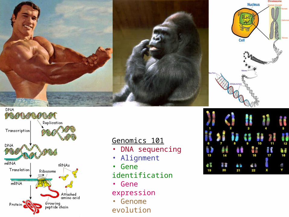
Genomics 101• DNA sequencing• Alignment• Gene identification• Gene expression• Genome evolution• …

Next Few Topics
• Gene Recognition
Finding genes in DNA with computational methods
• Large-scale alignment & multiple alignment
Comparing whole genomes, or large families of genes
• Gene Expression and Regulation
Measuring the expression of many genes at a time
Finding elements in DNA that control the expression of genes

Gene Recognition
Credits for slides:Marina AlexanderssonLior PachterSerge Saxonov

Reading
• GENSCAN
• EasyGene
• SLAM
• Twinscan
Optional:
Chris Burge’s Thesis

Gene expression
Protein
RNA
DNA
transcription
translation
CCTGAGCCAACTATTGATGAA
PEPTIDE
CCUGAGCCAACUAUUGAUGAA

Gene structure
exon1 exon2 exon3intron1 intron2
transcription
translation
splicing
exon = protein-codingintron = non-coding
Codon:A triplet of nucleotides that is converted to one amino acid

Where are the genes?Where are the genes?

In humans:
~22,000 genes~1.5% of human DNA

Finding Genes
1. Exploit the regular gene structureATG—Exon1—Intron1—Exon2—…—ExonN—STOP
2. Recognize “coding bias”CAG-CGA-GAC-TAT-TTA-GAT-AAC-ACA-CAT-GAA-…
3. Recognize splice sitesIntron—cAGt—Exon—gGTgag—Intron
4. Model the duration of regionsIntrons tend to be much longer than exons, in mammalsExons are biased to have a given minimum length
5. Use cross-species comparisonGene structure is conserved in mammalsExons are more similar (~85%) than introns

Approaches to gene finding
• Homology BLAST, Procrustes.
• Ab initio Genscan, Genie, GeneID.
• Hybrids GenomeScan, GenieEST, Twinscan, SGP, ROSETTA,
CEM, TBLASTX, SLAM.

Start codonATG
5’ 3’
Exon 1 Exon 2 Exon 3Intron 1 Intron 2
Stop codonTAG/TGA/TAA
Splice sites
1. Exploit the regular gene structure

Next Exon:Frame 0
Next Exon:Frame 1

2. Recognize “coding bias”
• Each exon can be in one of three framesag—gattacagattacagattaca—gtaag Frame 0ag—gattacagattacagattaca—gtaag Frame 1ag—gattacagattacagattaca—gtaag Frame 2
Frame of next exon depends on how many nucleotides are left over from previous exon
• Codons “tag”, “tga”, and “taa” are STOP No STOP codon appears in-frame, until end of gene Absence of STOP is called open reading frame (ORF)
• Different codons appear with different frequencies—coding bias

2. Recognize “coding bias”
Amino Acid SLC DNA codonsIsoleucine I ATT, ATC, ATALeucine L CTT, CTC, CTA, CTG, TTA, TTGValine V GTT, GTC, GTA, GTGPhenylalanine F TTT, TTCMethionine M ATGCysteine C TGT, TGCAlanine A GCT, GCC, GCA, GCG Glycine G GGT, GGC, GGA, GGG Proline P CCT, CCC, CCA, CCGThreonine T ACT, ACC, ACA, ACGSerine S TCT, TCC, TCA, TCG, AGT, AGCTyrosine Y TAT, TACTryptophan W TGGGlutamine Q CAA, CAGAsparagine N AAT, AACHistidine H CAT, CACGlutamic acid E GAA, GAGAspartic acid D GAT, GACLysine K AAA, AAGArginine R CGT, CGC, CGA, CGG, AGA, AGGStop codons Stop TAA, TAG, TGA
Can map 61 non-stop codons to frequencies & take log-odds ratios

atg
tga
ggtgag
ggtgag
ggtgag
caggtg
cagatg
cagttg
caggccggtgag

Biology of Splicing
(http://genes.mit.edu/chris/)

3. Recognize splice sites
(http://www-lmmb.ncifcrf.gov/~toms/sequencelogo.html)
Donor: 7.9 bitsAcceptor: 9.4 bits(Stephens & Schneider, 1996)

5’ 3’Donor site
Position
-8 … -2 -1 0 1 2 … 17
A 26 … 60 9 0 1 54 … 21C 26 … 15 5 0 1 2 … 27G 25 … 12 78 99 0 41 … 27T 23 … 13 8 1 98 3 … 25
3. Recognize splice sites

• WMM: weight matrix model = PSSM (Staden 1984)• WAM: weight array model = 1st order Markov (Zhang & Marr 1993)• MDD: maximal dependence decomposition (Burge & Karlin 1997)
Decision-tree algorithm to take pairwise dependencies into account
• For each position I, calculate Si = ji2(Ci, Xj)
• Choose i* such that Si* is maximal and partition into two subsets, until
• No significant dependencies left, or
• Not enough sequences in subset
Train separate WMM models for each subset
All donor splice sites
G5
not G5
G5G-1
G5
not G-1
G5G-1
A2
G5G-1
not A2
G5G-1
A2U6
G5G-1A2
not U6
3. Recognize splice sites

4. Model the duration of regions

GTCAGATGAGCAAAGTAGACACTCCAGTAACGCGGTGAGTACATTAA
exon exon exonintronintronintergene intergene
Hidden Markov Models for Gene Finding
Intergene State
First Exon State
IntronState

GTCAGATGAGCAAAGTAGACACTCCAGTAACGCGGTGAGTACATTAA
exon exon exonintronintronintergene intergene
Hidden Markov Models for Gene Finding
Intergene State
First Exon State
IntronState

TAA A A A A A A A A A A AA AAT T T T T T T T T T T T T T TG GGG G G G GGGG G G G GCC C C C C C
Exon1 Exon2 Exon3
duration
Duration HMM for Gene Finding
Duration Modeling
Introns: regular HMM states—geometric durationExons: special duration model
VE0,0(i) = maxd=1…D { Prob[duration(E0,0)=d]aIntron0,E0,0 j=i-d+1…ieE0,0(xj) }
where i is an admissible exon-ending state,D is restricted by the longest ORF
GENSCAN:Chris Burge and Sam Karlin, 1997
Best performing de novo gene finderHMM with duration modeling for Exon states

HMM-based Gene Finders
• GENSCAN (Burge 1997) Big jump in accuracy of de novo gene finding Currently, one of the best HMM with duration modeling for Exon states
• FGENESH (Solovyev 1997) Currently one of the best
• HMMgene (Krogh 1997)
• GENIE (Kulp 1996)
• GENMARK (Borodovsky & McIninch 1993)
• VEIL (Henderson, Salzberg, & Fasman 1997)

Better way to do it: negative binomial
• EasyGene:
Prokaryotic
gene-finder
Larsen TS, Krogh A
• Negative binomial with n = 3

GENSCAN’s hidden weapon
• C+G content is correlated with: Gene content (+) Mean exon length (+) Mean intron length (–)
• These quantities affect parameters of model
• Solution Train parameters of model in four
different C+G content ranges!

Evaluation of Accuracy
(Slide by NF Samatova)
Sensitivity (SN) Fraction of exons (coding nucleotides) whose boundaries are predicted exactly (that are predicted as coding)
•Specificity (Sp) Fraction of the predicted exons (coding nucleotides) that are exactly correct (that are coding)
•Correlation Coefficient (CC)
Combined measure of Sensitivity & Specificity Range: -1 (always wrong) +1 (always right)
TP FP TN FN TP FN TN
Actual
Predicted
Coding / No Coding
TNFN
FPTP
Pre
dic
ted
Actual
No
Co
din
g /
Co
din
g

Results of GENSCAN
• On the initial test dataset (Burset & Guigo) 80% exact exon detection
• 10% partial exons• 10% wrong exons
• In general
HMMs have been best in de novo prediction In practice they overpredict human genes by ~2x


