Alma Mater Studiorum Alma Mater Studiorum – Università di Bologna Università di Bologna DOTTORATO DI RICERCA IN Geofisica Ciclo XXVII Settore Concorsuale di afferenza: 04/A4 Settore Scientifico disciplinare:GEO/10 TITOLO TESI Turbulent Diffusion of the Geomagnetic Field and Dynamo Theories Presentata da: Enrico Filippi Coordinatore Dottorato Relatore Prof. Nadia Pinardi Dott. Angelo De Santis Correlatore Prof. Maurizio Bonafede Esame finale anno 2016
Transcript
Alma Mater Studiorum Alma Mater Studiorum –– Università di Bologna Università di Bologna
DOTTORATO DI RICERCA IN
Geofisica
Ciclo XXVII
Settore Concorsuale di afferenza: 04/A4 Settore Scientifico disciplinare:GEO/10
TITOLO TESI Turbulent Diffusion of the Geomagnetic Field and Dynamo
Theories
Presentata da: Enrico Filippi Coordinatore Dottorato Relatore Prof. Nadia Pinardi Dott. Angelo De Santis Correlatore Prof. Maurizio Bonafede
1.2.1 Toroidal and poloidal vectors. Free decay modes for a sphere . 141.3 Internal and external sources . . . . . . . . . . . . . . . . . . . . . . 161.4 Spatial and temporal spectra of the Geomagnetic Field . . . . . . . . 17
2 Random forcing in isotropic turbulence and Magnetohydrodynamics 192.1 A first approach to homogeneous isotropic turbulence . . . . . . . . . 192.2 Random Forcing and Turbulence in Magnetohydridynamics . . . . . . 20
3 Turbulent diffusive regime of the geomagnetic field during the last millen-nia 213.1 Magnetic induction equation and diffusion . . . . . . . . . . . . . . . 213.2 Global models analysis . . . . . . . . . . . . . . . . . . . . . . . . . 24
1.1 Reference frame for the magnetic field. I is the inclination or latitude.D is the declination or longitude (Figure by Parker, 2005). . . . . . . 11
1.2 Schematic representation of the different sources responsible for the Earth’s magnetic field. 121.3 Temperature vs depth (Figure by http://www.nhn.ou.edu/~jeffery/astro/astlec/lec011/earth_004_temperature.png).
131.4 Energy density vs n. . . . . . . . . . . . . . . . . . . . . . . . . . . . . . 17
3.1 ln (g10)2 vs t. The red parts of this graphic represent temporal in-
tervals longer than 100 years when ln (g10)2 decreased approximately
linearly with time; so we have decided to estimate τi by the data ofthese intervals. The g10 coefficients were synthesized by CALS7k modelexcept for the last red interval when the coefficients were synthesizedby IGRF model. . . . . . . . . . . . . . . . . . . . . . . . . . . . . . 28
3.2 Temporal trend of the geomagnetic field power on the Earth’s Surfaceand on the Core Mantle Boundary (CMB)(Figure by Korte and Con-stable, 2005). . . . . . . . . . . . . . . . . . . . . . . . . . . . . . . 29
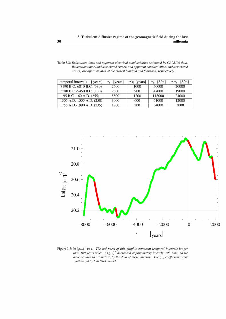
3.3 ln (g10)2 vs t. The red parts of this graphic represent temporal in-
tervals longer than 100 years when ln (g10)2 decreased approximately
linearly with time; so we have decided to estimate τi by the data ofthese intervals. The g10 coefficients were synthesized by CALS10k model. 30
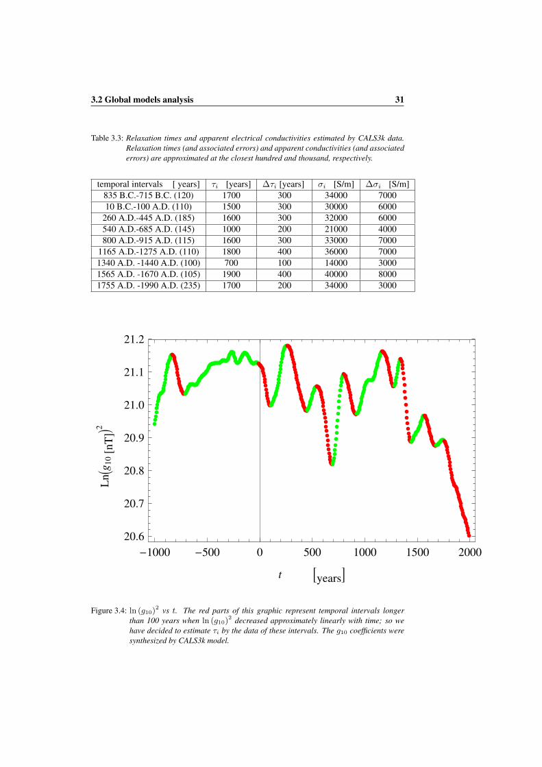
3.4 ln (g10)2 vs t. The red parts of this graphic represent temporal in-
tervals longer than 100 years when ln (g10)2 decreased approximately
linearly with time; so we have decided to estimate τi by the data ofthese intervals. The g10 coefficients were synthesized by CALS3k model. 31
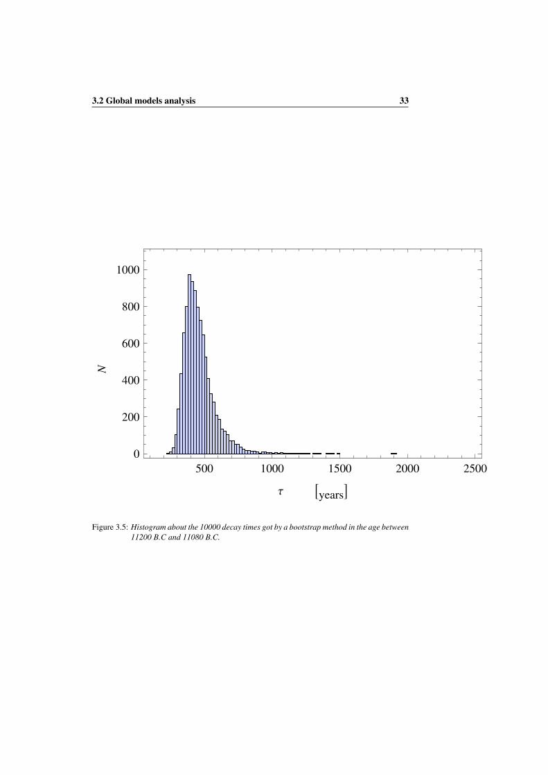
3.5 Histogram about the 10000 decay times got by a bootstrap method inthe age between 11200 B.C and 11080 B.C. . . . . . . . . . . . . . . 33
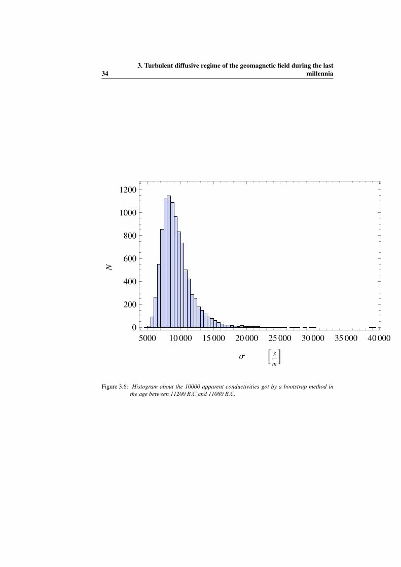
3.6 Histogram about the 10000 apparent conductivities got by a bootstrapmethod in the age between 11200 B.C and 11080 B.C. . . . . . . . . 34
3.7 Histogram about the 10000 decay times got by a bootstrap method inthe age between 6460 B.C and 6320 B.C. . . . . . . . . . . . . . . . 35
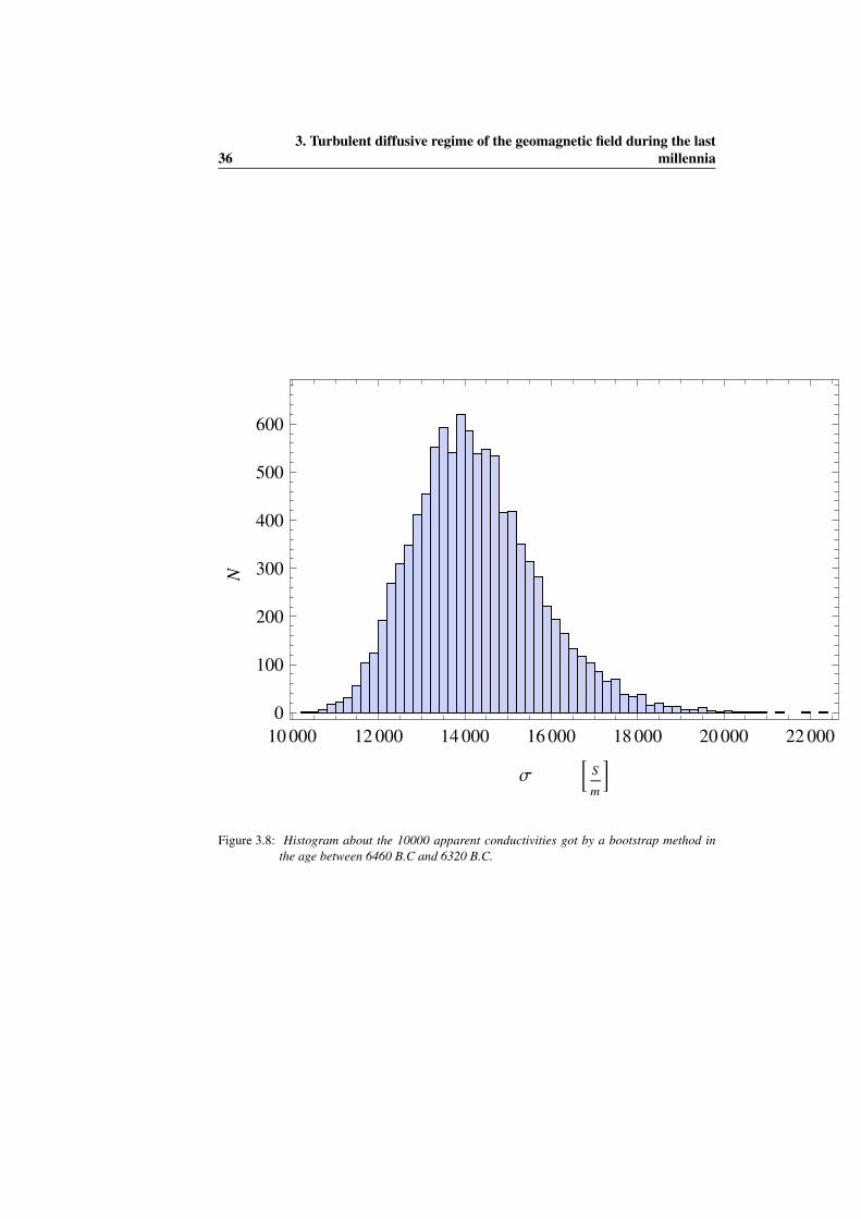
3.8 Histogram about the 10000 apparent conductivities got by a bootstrapmethod in the age between 6460 B.C and 6320 B.C. . . . . . . . . . 36
3.9 Histogram about the 10000 decay times got by a bootstrap method inthe age between 1750 A.D. and 1875 A.D. . . . . . . . . . . . . . . . 37
3.10 Histogram about the 10000 apparent conductivities got by a bootstrapmethod in the age between 1750 A.D. and 1875 A.D. . . . . . . . . . 38
4 LIST OF FIGURES
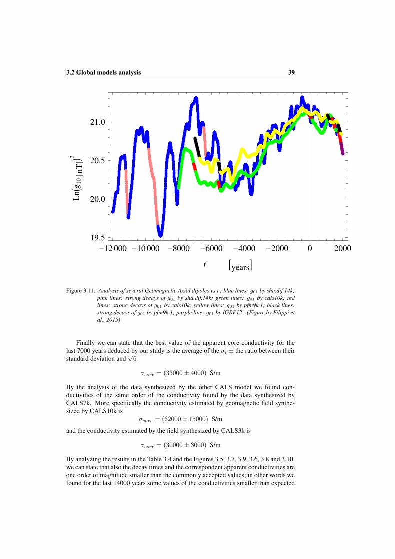
3.11 Analysis of several Geomagnetic Axial dipoles vs t ; blue lines: g01 bysha.dif.14k; pink lines: strong decays of g01 by sha.dif.14k; green lines:g01 by cals10k; red lines: strong decays of g01 by cals10k; yellow lines:g01 by pfm9k.1; black lines: strong decays of g01 by pfm9k.1; purpleline: g01 by IGRF12 . (Figure by Filippi et al., 2015) . . . . . . . . . 39
4.1 Maximum temporal variation of g01 in the ages between 1980 A.D.and 2015 A.D. (these coefficients are by IGRF12 model (Thebault etal., 2015)) . . . . . . . . . . . . . . . . . . . . . . . . . . . . . . . . 44
4.2 Maximum temporal variation of g01 in the ages between 1980 A.D.and 1990 A.D. (these coefficients are by CALS10k model (Korte et al.,2011)) . . . . . . . . . . . . . . . . . . . . . . . . . . . . . . . . . . 45
4.3 Maximum temporal variation of g01 in the ages between 1980 A.D.and 1990 A.D. (these coefficients are by CALS3k model (For referenceabout this modelKorte and Constable, 2003 and Korte et al., 2009)) . 46
List of Tables
1.1 Curie temperatures of some materials in the Earth (For references seee.g. Blaney, 2007, Heller, 1967, Kolel-Veetil and Keller, 2010, Pan etal., 2000) . . . . . . . . . . . . . . . . . . . . . . . . . . . . . . . . 12
3.1 Relaxation times and apparent electrical conductivities estimated byCALS7k and IGRF data. Relaxation times (and associated errors) andapparent conductivities (and associated errors) are approximated atthe closest hundred and thousand, respectively. . . . . . . . . . . . . 29
3.2 Relaxation times and apparent electrical conductivities estimated byCALS10k data. Relaxation times (and associated errors) and apparentconductivities (and associated errors) are approximated at the closesthundred and thousand, respectively. . . . . . . . . . . . . . . . . . . 30
3.3 Relaxation times and apparent electrical conductivities estimated byCALS3k data. Relaxation times (and associated errors) and apparentconductivities (and associated errors) are approximated at the closesthundred and thousand, respectively. . . . . . . . . . . . . . . . . . . 31
3.4 Relaxation times and apparent electrical conductivities estimated bySHA.DIF.14k data. Relaxation times (and associated errors) and ap-parent conductivities (and associated errors) are approximated at theclosest hundred and thousand, respectively. . . . . . . . . . . . . . . 32
6 LIST OF TABLES
Abstract
The thesis deals with the Dynamo Theories of the Earth’s Magnetic Field and mainlydeepens the turbulence phenomena in the fluid Earth’s core. Indeed, we think that thesephenomena are very important to understand the recent decay of the geomagnetic field.The thesis concerns also the dynamics of the outer core and some very rapid changesof the geomagnetic field observed in the Earth’s surface and some aspects regarding the(likely) isotropic turbulence in the Magnetohydrodynamics. These topics are related tothe Dynamo Theories and could be useful to investigate the geomagnetic field trends.
8 LIST OF TABLES
Introduction
The thesis deals with the Dynamo Theories of the Earth’s Magnetic Field and mainlydeepens the turbulence phenomena in the fluid Earth’s core. Indeed, we think thatthese phenomena are very important to understand the recent decay of the geomagneticfield. The thesis concerns also the dynamics of the outer core and some very rapidchanges of the geomagnetic field trend observed in the Earth’s surface and some aspectsregarding the (likely) isotropic turbulence in the Magnetohydrodynamics. These topicsare related to the Dynamo Theories and could be useful to investigate the geomagnetictrends.
In Chapter 1 we introduce the Magnetic Field of the Earth and the Dynamo Theo-ries. More specifically, we briefly describe the main sources of the Magnetic Field ofthe Earth, we recall Maxwell equations in the Earth core and we derive the MagneticInduction Equation by making some suitable geophysical approximations. We Finally,in a particular case, we discuss some properties and features of the geomagnetic fieldas the decay times.
The aim of Chapter 2 is to extend a methodology about Random Forcing in isotropicturbulence in order to understand better the dynamics of the fluid Earth’s Core. Weexplain some previous studies and computational methods aimed to study some tur-bulence problems. These methods use the "Random forcing" techniques in order toinvestigate on the isotropic turbulence of Navier-Stokes equation. The purpose is toadapt these methods to treat isotropic turbulence in Magnetohydrodynamics by mod-ifying in a suitable way some codes used by M. Maxey(see e.g.Ruetsch and Maxey,1991).
In Chapter 3 we deal with some turbulent dynamo theory problems. In other words,we discuss how some small scale phenomena affect the trend of the geomagnetic field.We study the temporal behaviour of the geomagnetic field in the last few millenniain the context of turbulent dynamo theory. We consider several global geomagneticmodels concerning up to 14000 years. In particular we analyze the recent trend of thedipolar geomagnetic field, in order to find some evidences for a turbulent diffusivity.This work contributes, in an original way, to improve the knowledge of the geodynamoturbulent regime and helps to understand how much of this regime can be observed inthe recent geomagnetic field. Moreover our approach uses a new method and our studyconcerns a temporal interval greater than the interval considered by previous works.
In Chapter 4 we consider some large scale dynamo theory problems. We use anoptimization method in order to estimate the rapid changes of the dipolar geomagneticfield. This method was firstly developped by P.W. Livermore, A. Fournier and YvesGallet ( Livermore et al., 2014) in order to evaluate the maximum of the intensityvariations and to search the links between the outer core dynamics and rapid changesof the geomagnetic field. Here we modify this method in a suitable way to our settingand we present the related results. This extension is new, flexible and it could have
10 Introduction
interesting applications.
Chapter 1
The Earth’s Magnetic Field:Dynamo Theories
1.1 IntroductionThe geomagnetic field is an important property of our planet and it is shared with otherplanets in the solar system and with the Sun itself. We can use the magnetic compassbecause the magnetic field is a vector quantity, so it has a magnitude and a direction;this feature requires to introduce a suitable reference frame to describe properly thegeomagnetic field as the following:
Gilbert’s earlier speculation. He was also responsible for beginning the measurement of the geomagnetic
field at globally distributed observatories, some of which are still running today.
Figure 1.1
The magnetic field is a vector quantity, possessing both magnitude and direction; at any point on Earth
a free compass needle will point along the local direction of the field. Although we conventionally think
of compass needles as pointing north, it is the horizontal component of the magnetic field that is directed
approximately in the direction of the North Geographic Pole. The difference in azimuth between magnetic
north and true or geographic north is known as declination (positive eastward). The field also has a vertical
contribution; the angle between the horizontal and the magnetic field direction is known as the inclination
and is by convention positive downward (see Figure 1.1). Three parameters are required to describe the
magnetic field at any point on the surface of the Earth, and the conventional choices vary according to
subfields of geomagnetism and paleomagnetism . Traditionally, the vector B at Earth’s surface is referred to
a right-handed coordinate system: north-east-down for x-y-z. But often instead of using the components in
this system, three numbers used are: intensity, B = |B|, declination, D, and inclination, I as shown in thesketch or D, H and Z; H , or equivalently Bh, is the projection of the field vector onto the horizontal plane
and Z, or equivalently Bz , is the projection onto the vertical axis. D is measured clockwise from North
and ranges from 0 → 360 (sometimes −180 → 180). I is measured positive down from the horizontal
and ranges from −90 → + 90 (because field lines can also point out of the Earth, indeed it is only in the
northern hemisphere that they are predominantly downward). From the diagram we have
H = BcosI; Bz = BsinI. (1)
2
Figure 1.1: Reference frame for the magnetic field. I is the inclination or latitude. D is thedeclination or longitude (Figure by Parker, 2005).
12 1. The Earth’s Magnetic Field: Dynamo Theories
If B is the magnitude of the geomagnetic field B, D is the declination and I is theinclination, by the Figure 1.1 we can easily deduce that
Bx = B cos I cos D
By = B cos I sin D
Bz = B sin I
1.2 Magnetic Induction EquationIn this section we deduce and analyze the Magnetic Induction Equation in a similarway as it is done in Gubbins and Roberts, (1987).
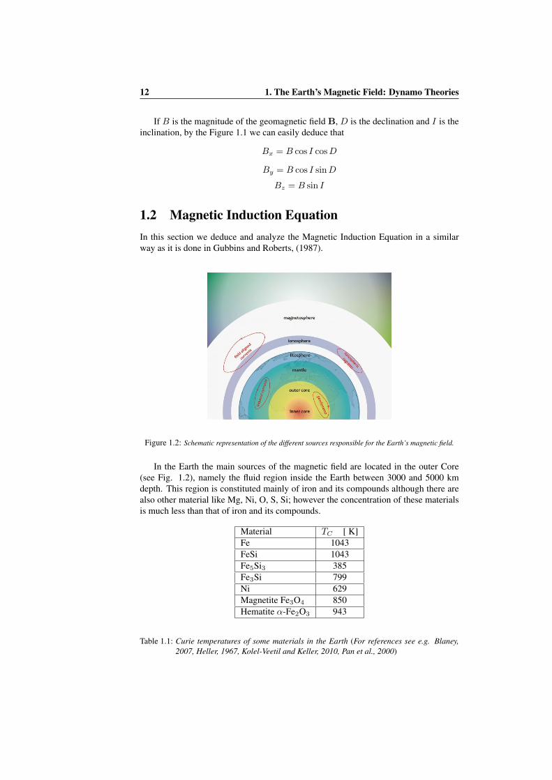
Figure 1.2: Schematic representation of the different sources responsible for the Earth’s magnetic field.
In the Earth the main sources of the magnetic field are located in the outer Core(see Fig. 1.2), namely the fluid region inside the Earth between 3000 and 5000 kmdepth. This region is constituted mainly of iron and its compounds although there arealso other material like Mg, Ni, O, S, Si; however the concentration of these materialsis much less than that of iron and its compounds.
Table 1.1: Curie temperatures of some materials in the Earth (For references see e.g. Blaney,2007, Heller, 1967, Kolel-Veetil and Keller, 2010, Pan et al., 2000)
1.2 Magnetic Induction Equation 13
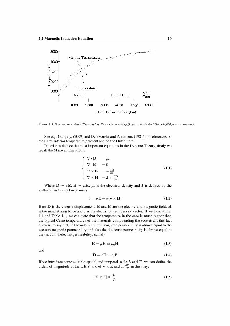
Figure 1.3: Temperature vs depth (Figure by http://www.nhn.ou.edu/~jeffery/astro/astlec/lec011/earth_004_temperature.png).
See e.g. Ganguly, (2009) and Dziewonski and Anderson, (1981) for references onthe Earth Interior temperature gradient and on the Outer Core.
In order to deduce the most important equations in the Dynamo Theory, firstly werecall the Maxwell Equations:
∇ · D = ρe
∇ · B = 0
∇×E = −∂B∂t
∇×H = J + ∂D∂t
(1.1)
Where D = εE, B = µH, ρe is the electrical density and J is defined by thewell-known Ohm’s law, namely
J = σE + σ(v ×B) (1.2)
Here D is the electric displacement, E and B are the electric and magnetic field, H
is the magnetizing force and J is the electric current density vector. If we look at Fig.1.4 and Table 1.1, we can state that the temperature in the core is much higher thanthe typical Curie temperatures of the materials compounding the core itself; this factallow us to say that, in the outer core, the magnetic permeability is almost equal to thevacuum magnetic permeability and also the dielectric permeability is almost equal tothe vacuum dielectric permeability, namely
B = µH µ0H (1.3)
andD = εE ε0E (1.4)
If we introduce some suitable spatial and temporal scale L and T , we can define theorders of magnitude of the L.H.S. and of ∇×E and of ∂B
∂tin this way:
|∇×E| ≈ EL
(1.5)
14 1. The Earth’s Magnetic Field: Dynamo Theories
and ∂B
∂t
≈BT
(1.6)
where B and E are the typical mean values of the magnetic and electric field. The IIIMaxwell’s equation and a comparison between (1.5) and (1.6) lead to:
EB ≈
L
T(1.7)
So, bearing in mind the (1.3), (1.4) and the (1.7) we can state that∂D
∂t
|∇×H| ≈ ε0µ0(L/T )2 (1.8)
But from electromagnetic theory ε0µ0 = 1/c2, where c is the light speed; the typicalgeomagnetic length-scales and time-scales allow us to say that the ratio (L/T ) is c(for references see e.g. Backus et al., 1996 and Parker, 2005); in other words in Geo-magnetism we can neglect the displacement current.
∇×H ≈ J (1.9)
The expression written above is called Magnetohydrodynamic approximation. By tak-ing the curl of the IV Maxwell’s equation and bearing in mind the (1.2), (1.3) and the(1.9) we obtain:
∂B
∂t=
1σµ0
∇2B +∇× (v ×B) (1.10)
The equation (1.10) is called Magnetic Induction Equation and it is the most im-portant equation in the Dynamo Theory and in Magnetohydrodynamics.
1.2.1 Toroidal and poloidal vectors. Free decay modes for a sphereThe B field is divergenceless, so it can be separated into toroidal and poloidal part.
B = ∇× ψT r +∇× (∇× ψP r) = BT + BP (1.11)
Now, it is convenient to use the spherical coordinates (r, θ,φ), where r is the radius, θis colatitude and φ is the latitude.
BT =
0,1
sin θ
∂ψT
∂φ,−∂ψT
∂θ
(1.12)
BP =
l2ψP
r,1r
∂2(rψP )∂θ∂r
,1
r sin θ
∂2(rψP )∂φ∂r
(1.13)
where l2 is the angular-momentum operator in quantum mechanics, namely
l2 ≡ −
1sin θ
∂
∂θ
sin θ
∂
∂θ
+
1sin2 θ
∂2
∂φ2
Note that the toroidal field BT cannot be measured on the Earth’s Surface, because itsradial component vanishes.
1.2 Magnetic Induction Equation 15
Now, if we consider the simple case where v = 0, the (1.10) is equal to the well-knowndiffusion equation
∂B
∂t= η∇2
B (1.14)
with η = 1µ0σ
; it is very easy to prove that any solution of the (1.14) can be written likethe (1.11) where ψT and ψP are solutions of the following equations:
∂ψT
∂t= η∇2ψT
∂ψP
∂t= η∇2ψP
(1.15)
The (1.15) can be solved by some standard techniques described e.g. in Gubbins andRoberts, (1987). After developping these techniques we can state that two solutions ofthe (1.15) are:
ψT (r, θ,φ, t) =∞
l=1
l
m=0
tml
(r)ylm(θ,φ)
ν
e−t/τνl (1.16)
ψP (r, θ,φ, t) =∞
l=1
l
m=0
pm
l(r)ylm(θ,φ)
ν
e−t/τνl (1.17)
where
ylm(θ,φ) =(2l + 1)(l − |m|)!
4π(l + |m|)!
1/2 12ll!
sinm θdl+|m|(cos2 θ − 1)l
d(cos θ)l+|m| eimφ
tml
= hlmjl
kT r
RC
pm
l= qlmjl
kP r
RC
and
τνl =R2
C
η(kνl)2(1.18)
where hlm and qlm are constants, jl are the Bessel functions of half-integer order,RC is the radius of the outer core, kT and kP are the solutions of the equations:
jl(kT ) = 0 (1.19)
jl−1(kP ) = 0 (1.20)
τνl are the decay times and each kνl is the ν-th solution of the equations (1.19), (1.20)Equations (1.18)-(1.20) can be easily derived according to Gubbins and Roberts,
(1987), by using the following property of the Bessel functions (see e.g. Abramowitzand Stegun, 1970)
jl(x) + (l + 1)
jl(x)x
= jl−1(x) (1.21)
and reminding these important continuity conditions of the electromagnetic fields:
16 1. The Earth’s Magnetic Field: Dynamo Theories
[n · B] = 0 su r = RN (1.22)
[n×B] = 0 su r = RN (1.23)
[n×E] = 0 su r = RN (1.24)
[n · J] = 0 su r = RN (1.25)
[n · E] = 0 su r = RN (1.26)
where [ ] denotes the jump across the Outer Core Surface.
1.3 Internal and external sourcesWe said in Section 1.2 that the main sources of the Geomagnetic Field are in the OuterCore. However, there are some relevant geomagnetic field sources also in the iono-sphere, the region of the upper atmosphere where the ionization is much greater than inthe low atmosphere. Indeed, this great ionization creates several electric currents (seeFig. 1.2). In other words, the main sources of the geomagnetic field are in the OuterCore (internal sources) and in the Ionosphere (external sources). From (1.9), we canformalize this fact in the following way:
∇×B(r, θ,φ) = 0 if RCMB ≤ r < Rion
∇×B(r, θ,φ) = µ0JC if RICB ≤ r < RCMB
∇×B(r, θ,φ) = µ0Jion if r ≥ Rion
(1.27)
where RCMB is the radius of the Outer Core, RICB is the radius of the Inner Core,Rion is the radius of the Ionosphere (by CMB we mean the Core Mantle Boundary,and by ICB the Inner Core Boundary). So, the B can be represented as a conservativefield, if RCMB ≤ r < Rion. This fact together with the II Maxwell’s equation, allowus to state that if RCMB ≤ r < Rion:
B = −∇V∇2V = 0V = Vint + Vext
(1.28)
where:
Vint = aNi
n=1
n
m=0
a
r
n+1(gnm cos(mφ) + hnm sin(mφ))Pm
n(cos θ) (1.29)
and
Vext = aNi
n=1
n
m=0
r
a
n
(qnm cos(mφ) + snm sin(mφ))Pm
n(cos θ). (1.30)
1.4 Spatial and temporal spectra of the Geomagnetic Field 17
1.4 Spatial and temporal spectra of the GeomagneticField
According to the contribution of De Santis et al., (2003), we can introduce the spatialand temporal spectra of the Geomagnetic Field. The spatial spectrum of the Geomag-netic Field and of its first temporal derivative B are:
B2 =
n
B2n B2
n = (n + 1)
n
m=0
g2
mn+ h2
mn
(1.31)
B2 =
n
B2n B2
n = (n + 1)
n
m=0
g2
mn+ h2
mn
(1.32)
where gmn and hmn are the coefficients defined at the end of the previous section andgmn and hmn are their time derivatives. It is possible to express:
B2n = keαn (1.33)
B2n = keα
n (1.34)
where k, k, α and α are suitable parameters. It is important to note that by means ofthe geomagnetic spatial spectrum we can distinguish core from crustal fields (see e.g.De Santis et al., 2016 ).
!!!
!"!!
#$%&'!()'&!
('$*%!
Figure 1.4: Energy density vs n.
18 1. The Earth’s Magnetic Field: Dynamo Theories
By the (1.33) and (1.34) we can define the temporal spectrum in the following way:
B2n ∝ (en)α = ω−γ
n(1.35)
where
ωn =
k
ke−(α−α
)n/2 and γ =2α
α− α.
Chapter 2
Random forcing in isotropicturbulence andMagnetohydrodynamics
In this chapter we describe a methodology about Random Forcing in isotropic turbu-lence in order to highlight the dynamics of the fluid Earth’s Core. We explain someprevious studies and computational methods aimed to study some turbulence prob-lems. These methods use the "Random forcing" techniques in order to investigate onthe isotropic turbulence of Navier-Stokes equation. Our aim is to discuss how muchis important the the turbulence in Magnetohydrodynamics and how can be observed inthe trend of the Geomagnetic Field.
2.1 A first approach to homogeneous isotropic turbu-lence
There are several works that used the Random Forcing methods to study the rotationalform of the Navier-Stokes equation, namely:
∂v
∂t+ ω × v = −∇
p
ρ+
12|v|2
+ ν∇2
v (2.1)
Firstly, we briefly explain a method to study a problem in homogeneous isotropic tur-bulence developped in Ruetsch and Maxey, (1991). This method for simplicity’ s sakeuses a simplified geometry. It considers a cube of side L = 2π, that is discretizedinto N3 grid points, with periodic boundary conditions in all three directions. The gridpoints in physical space are defined as
(xi, yj , zk) =
L
Ni,
L
Nj,
L
Nk
(2.2)
where i, j, k = 1, 2, ..., N . The grid points in Fourier space, or wave-number compo-nents, are of the form:
ki = ±ni(2π/L) (2.3)
20 2. Random forcing in isotropic turbulence and Magnetohydrodynamics
where ni = 0, 1, 2, ..., N/2 for i = 1, 2, 3. Data specified at the physical grid points,such as the velocity field v(r, t), can be transformed to Fourier space by
v(k, t) =1
N3
r
v(r, t) exp(−ik · r) (2.4)
and the Fourier coefficients v(k, t) can be transformed back to physical space by
v(r, t) =1
N3
k
v(k, t) exp(ik · r) (2.5)
Such transformations are of order (N3)2 operations, but with the use of FFT’s theoperation count is reduced to N3 ln(N3) operations.
2.2 Random Forcing and Turbulence in Magnetohydri-dynamics
A possible application to Magnetohydrodynamics is to use the method, described inthe section 2.1, in order to study a system like this:
∂v∂t
+ ω × v = −∇
p
ρ+ 1
2 |v|2
+ ν∇2v + 1
µ0(∇×B)×B
∂B∂t
= 1σµ0∇2
B +∇× (v ×B)(2.6)
In other words, if we suppose that in the velocity field of the outer core, there is arandom part, that creates a turbulence we can try to solve, also under suitable approxi-mations, the system (2.6) and then compare the Geomagnetic Field, we found with theobserved Geomagnetic Field; this , can help us to understand whether the Outer Earth’Core is in a turbulent regime or not.There is also another way to investigate on the (supposed) turbulence in the core: weconsider the the main equations of the Dynamo Theories when the geodynamo is ina turbulent state, we put, atfer assuming some hypothesis, these equations in a morehandy way, and then we deduce from then what we expect about the behaviour of thegeomagnetic field in these turbulent conditions. Finally, we analyze the trend of thegeomagnetic field in order to check whether this trend is consistent with a "turbulentgeodynamo" or not. For logistical reasons, we chose to use this second way in order toinvestigate on the turbulence in the core; we present the methodology and the results inChapter 3.
Chapter 3
Turbulent diffusive regime ofthe geomagnetic field during thelast millennia
In this chapter we report the study of the temporal behaviour of the geomagnetic fieldin the last few millennia in the context of turbulent dynamo theory, in order to estab-lish whether the corresponding geomagnetic field is in a turbulent diffusivity regimeor not. In the positive case, this would support the possibility of an imminent geo-magnetic reversal of the present polarity of the field, as some recent papers prospectedthis possible event (Hulot et al., 2002; De Santis et al., 2004; De Santis, 2007; but seealso Constable and Korte, 2006 ). To do this, in the next section, in order to introducethe problem and to explain the meaning of what we call “turbulent diffusivity”we willrecall the foundations of the theory of the turbulent phenomena in the Earth’s fluid corei.e. how the geomagnetic field is generated and sustained. This turbulence is a conse-quence of the strong non-linear interactions among the physical quantities involved inthe generation of the planetary magnetic field as shown in section 3.1. In the section 3.2we will analyse several global models to look at some properties of the diffusive partof the field in the last years: more specifically we analyse models of the geomagneticfield for the last 3000, 7000, 10000 and 14000 years. Finally, in the section 5 we willattempt to establish a connection between our results and the theoretical predictions ofa turbulent geomagnetic field in the Earth’s outer core, together with some discussionabout possible improvements of the present work.
3.1 Magnetic induction equation and diffusionIn the outer core the dynamics of the Earth’s magnetic field B is determined by thewell-known magnetic induction equation, already derived in Section 1.2
∂B
∂t= η∇2
B +∇× (V ×B) (3.1)
where V is the velocity field of the fluid core, η = 1σµ0
is called “magnetic diffusivity”or “coefficient of ohmic diffusion of the magnetic field”, σ is the electrical conductivityand µ0 is the vacuum magnetic permeability. The first part of the R.H.S. of the (3.1) is
223. Turbulent diffusive regime of the geomagnetic field during the last
millennia
a diffusive term, namely a term that gradually extinguishes the field; the second part ofthe R.H.S. is the “inductive term” and may contribute in producing (and possibly in-tensifying) new field. However, in some particular turbulence situations, the inductiveterm may increase the diffusion: we will better explain this concept below in a simi-lar way as it was explained by different authors (Moffatt, 1978; Rädler, 1968a; Rädler,1968b). When we have a turbulent situation the detailed properties of the main physicalquantities (B, V, etc.) are too complicated for either analytical description or obser-vational determination, so we have to determine these in terms of their given statistical(i.e. average) properties. First we introduce some suitable spatial and temporal scales,L and T , respectively. L is a ’global’ spatial scale, namely is of the same order as thelinear dimension of the region occupied by the conducting fluid: L = O(RC), whereRC is the radius of the outer core. T is the time-scale of variation of the various fieldscomposing the whole geomagnetic field produced in the outer core. The turbulencephenomena are generally confined in a length-scale l0 L and in a temporal scale t0 T . We may also define two intermediate scales a, t1 satisfying
l0 a L
t0 t1 T
So we can reasonably suppose that in a sphere of radius a or in a time t1 the mag-netic and velocity fields are weakly varying. Therefore we can, in general, define thefollowing averages for a certain quantity F (r, t)
F (r, t)a =3
4πa3
|r|<a
F (r + r, t)dr (3.2)
F (r, t)t1 =1
2t1
t1
−t1
F (r, t + τ )dτ (3.3)
In the next considerations we will not specify if we are making a temporal or spatialaverage; so we will not use the suffix a or t1, and from now on we use the more compactnotation
F = F and the following relations:
F = F + F , F = F , F = 0
F + G = F + G, FG = FG, FG = 0
FG = F G + F G
where G is another fluctuating field. Some of the previous relations hold only in anapproximate sense (as in the asymptotic limits l0/L → 0 and t0/T → 0). The aver-aging operator commutes with the differential and integration operators in both spaceand time.
Having thus defined a mean, either the velocity or the magnetic field may be sepa-rated into mean and fluctuating parts:
V(r, t) = V0(r, t) + v(r, t), v = 0 (3.4)
B(r, t) = B0(r, t) + b(r, t), b = 0 (3.5)
3.1 Magnetic induction equation and diffusion 23
where V0 and B0 have longer time and space scales than those of their associated fluc-tuating parts. By means of (3.4) and (3.5) we can decompose the magnetic inductionequation (3.1) into its mean and fluctuating parts:
∂B0
∂t= ∇× (V0 ×B0) +∇×∆ + η∇2
B0 (3.6)
∂b
∂t= ∇× (v ×B0) +∇× (V0 × b) + η∇2
b +∇×C (3.7)
with∆ = v × b
andC = v × b−∆
The term ∆, sometimes called mean electromotive force, is the most important partof the equation (3.7) because it describes the coupling between the fluctuating velocityand magnetic field; as we will show in more detail in the Appendix A, this term maybe developed as a series involving temporal and spatial derivatives of B0 and may berepresented as a sum of a power series of ascending powers of |v|n with n ≥ 2. Thesemanipulations are performed in order to rewrite in this manner the equation (3.6)
∂B0
∂t= ∇× (V0 ×B0) + (η + β)∇2
B0 + ... (3.8)
with β > 0, that we call "turbulent diffusivity " (see Appendix A).Therefore, as mentioned at the beginning of section 3.1, in particular turbulent
situations the inductive term may generate a “turbulent diffusivity”, namely it mayincrease the diffusion whereas, as we have reminded at the beginning of this section, inother conditions it may intensify the field. This phenomenon is also called “β-effect”(see e.g. Gruzinov and Diamond, 1994 or Leprovost and Kim, 2003). The fact thatthese inductive and diffusive terms of (3.1) are in cooperation or in competition, is aninteresting aspect of the Earth’s magnetic field. This interplay between cooperation andcompetition is a typical feature of complex systems, as it is explained for example inDe Santis (2009): therefore, in this sense, the geomagnetic field may be considered acomplex system (see also Baranger, 2001 for a general definition of a complex system).In the Appendix A we will derive also the following special case, at the order O(|v|2),of the (3.8) for each i-th component of the geomagnetic field :
∂Bi
∂t= (η +
13|v|2c(00))∇2Bi +
c(00)
3
∂|v|2∂xj
∂Bi
∂xj
− ∂|v|2∂xj
∂Bj
∂xi
+
+a(00)
3
Bi∇2|v|2 +
∂Bi
∂xj
∂|v|2∂xj
−Bj
∂2|v|2∂xj∂xi
+
+a(01)
3
∂2|v|2∂xj∂xi
∂Bj
∂t−∇2|v|2 ∂Bi
∂t− ∂|v|2
∂xj
∂2Bi
∂xj∂t
+ ... (3.9)
where the Einstein summation convention on the repeated indices is adopted; the coef-ficients a(00), a(01), c(00) depend on the geometry of the outer core and on the turbulentvelocity field and the term c(00) is connected with β; this expression, as we will sayin the section 5, might be a good starting point for future developments of the analysisdescribed in the next section.
243. Turbulent diffusive regime of the geomagnetic field during the last
millennia
3.2 Global models analysisIn this section we report the analysis of some global models of the geomagnetic field.In particular, we analyse 3 types of CALS models: CALS3k (see Korte and Constable,2003 and Korte et al., 2009), CALS7k (Korte and Constable, 2005) and CALS10k (Ko-rte et al., 2011); these models cover the last 3000, 7000 and 10000 years, respectively.Then, we analyze the SHA.DIF.14k model (Pavón-Carrasco et al., 2014) that covers14000 years and pfm9k.1 model (Nilsson et al., 2014) that covers 9000 years. We alsoanalyse the IGRF model to have a more detailed look at the last 100 years (Finlay etal., 2010). Our main purpose was to estimate the relaxation times at epochs when thegeomagnetic field was significantly decaying. First, as a simple working hypothesis,we suppose that when the field is in this specific situation only the diffusive term ofequation (3.1) will be present. Second, we analyse the typical time scales of the cor-responding geomagnetic dipole field decay. We would then expect that the relaxationtimes are those typical of a diffusive regime. If we do not find this, (as actually it willbe) we will interpret the results in terms of the presence of some "turbulent diffusivity".More discussion on these aspects will be given below.
3.2.1 Paleomagnetic and IGRF models
The CALS models are continuous global models of the geomagnetic field defined asspherical harmonics in space of the scalar magnetic potential and splines functions inspace. The CALS3k is valid from 1000 B.C. to 1990 A.D.(see Korte and Constable,2003 and Korte et al., 2009). This model is based on all available archeomagnetic andsediment data, without a priori quality selection; it currently constitutes the best globalrepresentation of the past field in its time of validity. Relative intensities from sedi-ment cores have been calibrated by a model based on archeomagnetic data or by usingarcheomagnetic data from nearby locations where available, and have subsequentlybeen used together with the sediment directional records. The CALS7k (Korte andConstable, 2005) is derived using a great number of archeomagnetic and paleomag-netic data covering the last 7000 years. The CALS10k is an average of 2000 individualmodels obtained by a bootstrap statistical approach based on data of the last 10 mil-lennia. The data used to develop it come from two distinct kinds of materials: rapidlyaccumulated sediments which preserve a post-depositional magnetic remanence, andmaterials which acquire a thermal remanent magnetization (Korte et al., 2011).The SHA.DIF.14k model is based on archaeomagnetic and lava flow data, avoiding theuse of lake sediment data. The remanent acquisition time for the archaeomagnetic andvolcanic lava flow material is nearly instantaneous. This feature allows to get a modelwith an unprecedented temporal resolution on the past evolution of the Earth’s mag-netic field.The pfm9k.1 is a spherical harmonic geomagnetic model covering the past 9000 years.It is based on magnetic field directions and intensity stored in archaeological artefacts,igneous rocks and sediment records. A new modelling strategy introduces alternativedata treatments with a focus on extracting more information from sedimentary data. Toreduce the influence of a few individual records all sedimentary data are resampled in50-yr bins, which also means that more weight is given to archaeomagnetic data dur-ing the inversion. The sedimentary declination data are treated as relative values andadjusted iteratively based on prior information. Finally, an alternative way of treatingthe sediment data chronologies has enabled us to both assess the likely range of ageuncertainties, often up to and possibly exceeding 500 yr and adjust the timescale of
3.2 Global models analysis 25
each record based on comparisons with predictions from a preliminary model.The IGRF is a spherical harmonic model of the Earth’s main magnetic field used widelyin studies of the Earth’s deep interior, its crust, ionosphere and magnetosphere. It pro-vides the Gauss coefficients from 1900 A.D. to the present times and is based on manymagnetic data from land observatories around the world and, more recently, from satel-lites (like Ørsted launched 1999, CHAMP launched 2000). For references about theversion of IGRF we have used see Finlay et al. (2010); for references about an earlierversion of the IGRF model see Maus et al. (2005a; 2005b).All above models represent the magnetic field as a conservative field, because they aremodels of the global magnetic field in source-free regions at the Earth’s surface andabove:
B = −∇
aNmax
n=1
n
m=0
a
r
n+1(gnm cos(mφ) + hnm sin(mφ))Pm
n(cos θ)
(3.10)where a is the Earth mean radius, r is the distance from the centre of the Earth, θ is thecolatitude and φ is the longitude, n and m, that ∈ N, are the spherical harmonic degreeand order, respectively. Pm
nare the so-called associate Legendre functions, namely
Pm
n=
12nn!
sinm θdn+m(cos2 θ − 1)n
d(cos θ)n+m(3.11)
The functions cos(mφ)Pm
nand sin(mφ)Pm
n, usually called spherical harmonics, have
the following orthogonality property 2π
0dφ
π
0Pm
n
cos(mφ)sin(mφ)
P l
k
cos(lφ)sin(lφ)
sin θdθ =
2mπ(n + m)!(2n + 1)(n−m)!
δlmδkn
(3.12)
where 0 = 2 and m = 1 if m > 0; with
cos(pφ)sin(pφ)
we want only remind that
2π
0 cos(pφ) sin(pφ)dφ = 0 ∀ p, p ∈ N.
The development of a Paleomagnetic model, like the models cited above, can besummarized in the following steps (for reference see e.g De Santis et al., 2016):
1. In terms of Spherical Harmonic Analysis (SHA), the internal potential of thegeomagnetic field can be established as:
Vint = aNi
n=1
n
m=0
a
r
n+1(gnm cos(mφ) + hnm sin(mφ))Pm
n(cos θ) (3.13)
2. The magnetic field components can be represented by the negative gradient ofthe potential:
B = −∇V = −∇ (Vint + Vest) (3.14)
3. Any scalar element d (e.g. total intensity ) of the geomagnetic field is expressedas a non-linear function f and depends on the time-dependent SH model coeffi-cients m:
d = f(m) + ε (3.15)
we used the "vector" m in the (3.15), because a function d in general depends onall m coefficients
263. Turbulent diffusive regime of the geomagnetic field during the last
millennia
4. The regularized weighted least square inversion applying the Newton-Raphsoniterative approach:
mi+1 = mi +“
Ai · Ce
−1Ai + α · Ψ + τ · Φ
”−1 “Ai
· Ce−1
γi − α · Ψ · mi − τ · Φ · mi
”
(3.16)
5. The Ψ and Φ matrices are the spatial and temporal regularization norms, respec-tively, with damping parameters α and τ :
Ns = α · Ψ =α
te − ts
1Ω0
te
ts
Ω|B|2dΩdt (3.17)
NT = τ · Φ =τ
te − ts
1Ω0
te
ts
Ω
∂2Br
∂t2
2
dΩdt (3.18)
3.2.2 Time scales, turbulent diffusivity and apparent core conductivity
In the data analysis we have used only the term proportional to the dipolar power(g10)2, instead of the term proportional to the total power
n(n + 1)
m
(gnm)2 +(hnm)2, for two reasons:
1. If we compare Figure 3.1 and Figure 3.2 we can see that the behaviours of bothterms (dipolar and total powers) are similar. This is because CALS7k modelprobably underestimates gnm with n > 1.
2. For our aims it is enough to use only g10 because that is the leading term ofthe total power of the field and it is important for defining the polarity of themagnetic field.
After drawing the graph in Figure 3.1, we supposed that in some temporal intervals, atleast longer than 100 years, characterised by a clear dipolar field decay the “dynamoeffect”, namely the intensification of the field due to the inductive term of magneticinduction equation, was negligible with respect to the ohmic diffusion of magneticfields. Therefore, for these intervals (here indicated in chronological order as i=1,...,6)we have supposed, in accordance with the diffusive term of the (3.1), a decay law ofthis type
g10(t) = g10(0)e−t/τi (3.19)
with
τi =R2
Cµ0σi
(k21)2(3.20)
where τi is the longest dipolar relaxation time of the i-th interval, RC is the outer coreradius and k21 is the least non-zero solution of the Bessel function J1/2(x) which isthe radial part of the solution of degree n = 1 of the heat equation/diffusive part of themagnetic induction equation; σi is the corresponding apparent electrical conductivityof the core, supposed solid and with the only diffusion process acting. It is for thisreason that we call σi "apparent" electrical conductivity. For references about the (3.20)see for example Gubbins and Roberts (1987) or Yukutake (1968) while for referencesabout Bessel functions see for example Abramowitz and Stegun, (1970). From (3.20)we can easily deduce
σi =τi (k21)
2
µ0R2C
(3.21)
3.2 Global models analysis 27
that was used to calculate σi from each τi.We performed several fits over the logarithm of the square of g10 coefficient at
different values of t; so we have written ln (g10)2 vs t in the Figs. 3.1, 3.3 and 3.4; the
argument of the logarithm in these graphs is not dimensionless but given in nT2.In order to estimate the errors on the τi and σi we bore in mind that the data synthesizedby the CALS7k model improve their quality in time, i.e. they are more precise in therecent centuries than in the earlier centuries (De Santis and Qamili, 2010). So we havedone the following assumptions on the relative errors on the τi
1. 40% concerning the age 5000 B.C.-4800 B.C.
2. 30% concerning the age 4465 B.C.-4360 B.C.
3. 30% concerning the age 2075 B.C.-1935 B.C.
4. 20% concerning the age 545 B.C.-415 B.C.
5. 20% concerning the age 580 A.D.-770 A.D.
6. 10% concerning the age 1900 A.D.-2010 A.D.
In practice this will mean that relaxation times (and associated errors) and apparentconductivities (and associated errors) are approximated at the closest hundred andthousand, respectively. We have done the same assumptions to perform the simula-tions using CALS3k and CALS10k models (see tables 3.2 and 3.3). In the next pagesthere are some figures and tables that summarize the results of our analysis.
283. Turbulent diffusive regime of the geomagnetic field during the last
millennia
!5000 !4000 !3000 !2000 !1000 0 1000 200019.6
19.8
20.0
20.2
20.4
20.6
20.8
21.0
t !years"
Ln#g
10$n
T%&2
Figure 3.1: ln (g10)2 vs t. The red parts of this graphic represent temporal intervals longer
than 100 years when ln (g10)2 decreased approximately linearly with time; so we
have decided to estimate τi by the data of these intervals. The g10 coefficients weresynthesized by CALS7k model except for the last red interval when the coefficientswere synthesized by IGRF model.
3.2 Global models analysis 29
Figure 3.2: Temporal trend of the geomagnetic field power on the Earth’s Surface and on theCore Mantle Boundary (CMB)(Figure by Korte and Constable, 2005).
Table 3.1: Relaxation times and apparent electrical conductivities estimated by CALS7k andIGRF data. Relaxation times (and associated errors) and apparent conductivities(and associated errors) are approximated at the closest hundred and thousand, re-spectively.
303. Turbulent diffusive regime of the geomagnetic field during the last
millennia
Table 3.2: Relaxation times and apparent electrical conductivities estimated by CALS10k data.Relaxation times (and associated errors) and apparent conductivities (and associatederrors) are approximated at the closest hundred and thousand, respectively.
95 B.C.-160 A.D. (255) 5800 1200 118000 240001305 A.D.-1555 A.D. (250) 3000 600 61000 120001755 A.D.-1990 A.D. (235) 1700 200 34000 3000
!8000 !6000 !4000 !2000 0 2000
20.2
20.4
20.6
20.8
21.0
t !years"
Ln#g
10$n
T%&2
Figure 3.3: ln (g10)2 vs t. The red parts of this graphic represent temporal intervals longer
than 100 years when ln (g10)2 decreased approximately linearly with time; so we
have decided to estimate τi by the data of these intervals. The g10 coefficients weresynthesized by CALS10k model.
3.2 Global models analysis 31
Table 3.3: Relaxation times and apparent electrical conductivities estimated by CALS3k data.Relaxation times (and associated errors) and apparent conductivities (and associatederrors) are approximated at the closest hundred and thousand, respectively.
260 A.D.-445 A.D. (185) 1600 300 32000 6000540 A.D.-685 A.D. (145) 1000 200 21000 4000800 A.D.-915 A.D. (115) 1600 300 33000 7000
1165 A.D.-1275 A.D. (110) 1800 400 36000 70001340 A.D. -1440 A.D. (100) 700 100 14000 30001565 A.D. -1670 A.D. (105) 1900 400 40000 80001755 A.D. -1990 A.D. (235) 1700 200 34000 3000
!1000 !500 0 500 1000 1500 2000
20.6
20.7
20.8
20.9
21.0
21.1
21.2
t !years"
Ln#g
10$n
T%&2
Figure 3.4: ln (g10)2 vs t. The red parts of this graphic represent temporal intervals longer
than 100 years when ln (g10)2 decreased approximately linearly with time; so we
have decided to estimate τi by the data of these intervals. The g10 coefficients weresynthesized by CALS3k model.
323. Turbulent diffusive regime of the geomagnetic field during the last
millennia
In the table below we report the results from the analysis of SHA.DIF.14k.
Table 3.4: Relaxation times and apparent electrical conductivities estimated by SHA.DIF.14kdata. Relaxation times (and associated errors) and apparent conductivities (and as-sociated errors) are approximated at the closest hundred and thousand, respectively.
We estimated the errors in this table, by a gaussian bootstrap method with 10000iterations. We used also this gaussian bootstrap method to estimate the errors, becauseit is a robust method widely used in geomagnetism (See e.g Korte et al., 2011 or Pavón-Carrasco et al., 2014) and there are several articles that highlight the importance of thefact that the statistics of the geophysical data is gaussian (see e.g Constable and Parker,1988). In the next pages there are some histograms about the relaxation times and the"apparent conductivities" got by the bootstrap method.
3.2 Global models analysis 33
500 1000 1500 2000 2500
0
200
400
600
800
1000
! !years"
N
Figure 3.5: Histogram about the 10000 decay times got by a bootstrap method in the age between11200 B.C and 11080 B.C.
343. Turbulent diffusive regime of the geomagnetic field during the last
Figure 3.6: Histogram about the 10000 apparent conductivities got by a bootstrap method inthe age between 11200 B.C and 11080 B.C.
3.2 Global models analysis 35
500 600 700 800 900 1000 1100
0
100
200
300
400
500
600
! !years"
N
Figure 3.7: Histogram about the 10000 decay times got by a bootstrap method in the age be-tween 6460 B.C and 6320 B.C.
363. Turbulent diffusive regime of the geomagnetic field during the last
millennia
10 000 12 000 14 000 16 000 18 000 20 000 22 000
0
100
200
300
400
500
600
! ! S
m
"
N
Figure 3.8: Histogram about the 10000 apparent conductivities got by a bootstrap method inthe age between 6460 B.C and 6320 B.C.
3.2 Global models analysis 37
2000 3000 4000 5000 6000 7000
0
200
400
600
800
1000
! !years"
N
Figure 3.9: Histogram about the 10000 decay times got by a bootstrap method in the age be-tween 1750 A.D. and 1875 A.D.
383. Turbulent diffusive regime of the geomagnetic field during the last
millennia
40 000 60 000 80 000 100 000 120 000 140 000
0
200
400
600
800
1000
! ! S
m
"
N
Figure 3.10: Histogram about the 10000 apparent conductivities got by a bootstrap method inthe age between 1750 A.D. and 1875 A.D.
3.2 Global models analysis 39
!12 000 !10 000 !8000 !6000 !4000 !2000 0 2000
19.5
20.0
20.5
21.0
t !years"
Ln#g
10$n
T%&2
Figure 3.11: Analysis of several Geomagnetic Axial dipoles vs t ; blue lines: g01 by sha.dif.14k;pink lines: strong decays of g01 by sha.dif.14k; green lines: g01 by cals10k; redlines: strong decays of g01 by cals10k; yellow lines: g01 by pfm9k.1; black lines:strong decays of g01 by pfm9k.1; purple line: g01 by IGRF12 . (Figure by Filippi etal., 2015)
Finally we can state that the best value of the apparent core conductivity for thelast 7000 years deduced by our study is the average of the σi ± the ratio between theirstandard deviation and
√6
σcore = (33000 ± 4000) S/m
By the analysis of the data synthesized by the other CALS model we found con-ductivities of the same order of the conductivity found by the data synthesized byCALS7k. More specifically the conductivity estimated by geomagnetic field synthe-sized by CALS10k is
σcore = (62000 ± 15000) S/m
and the conductivity estimated by the field synthesized by CALS3k is
σcore = (30000 ± 3000) S/m
By analyzing the results in the Table 3.4 and the Figures 3.5, 3.7, 3.9, 3.6, 3.8 and 3.10,we can state that also the decay times and the correspondent apparent conductivities areone order of magnitude smaller than the commonly accepted values; in other words wefound for the last 14000 years some values of the conductivities smaller than expected
403. Turbulent diffusive regime of the geomagnetic field during the last
millennia
So the found apparent core conductivities for the last 14000 years are, at least, oneorder of magnitude smaller than the commonly accepted values (see e.g. Gubbins andRoberts, 1987; Stacey and Loper, 2007; Pozzo et al., 2012 and the articles cited in thosepapers); this fact would have interesting implications as we will explain in Chapter 5 .
Chapter 4
Outer Core Dynamics and rapidintensity changes
In this chapter we use an interesting large scale method in order to estimate the rapidchanges of the dipolar geomagnetic field. This method was developped by P.W. Liv-ermore, A. Fournier and Yves Gallet and it is described in the paper Livermore et al.,(2014). We describe this method and then we present the results got by an extension ofthis method.
4.1 Introduction
The work described in Livermore et al., (2014) gives an estimation of the maximumtemporal variation of the Geomagnetic Field in some epochs by the Lagrange multi-pliers technique. The unique constraint assumed is that the root-mean-squared (rms)flow speed on the Core Mantle Boundary (CMB) is 13 km/yr (Holme, 2007). Thisconstraint is a results of several simulations performed on some geomagnetic models.In these models there are two fundamental assumptions:
1. The Geomagnetic Field is in the frozen-flux condition, namely the first term ofthe R.H.S of the (1.10) vanishes.
2. The flow of the liquid core is tangentially geostrophic, namely∇H · (v cos θ) =0, where∇H is the "horizontal divergence" and v is the velocity field of the outercore.
If we consider only short-time intervals, the Frozen-Flux hypothesis is reasonable, be-cause the diffusive effects are more effective after long-time intervals. If the gravity isfully radial the condition about the tangentially geostrophic flow is satisfied. The OuterCore is more spherical than the Earth’s Surface, so it is quite correct to assume thatthe gravity is fully radial on the CMB. So, we can state that it is a good approximationto assume the constraint that the root-mean-squared flow speed on the Core MantleBoundary (CMB) is 13 km/yr.
42 4. Outer Core Dynamics and rapid intensity changes
4.2 MethodologyThe geomagnetic intensity at S site is given by
F = |B| =
B2r
+ B2θ
+ B2φ
(4.1)
sodF
dt=
1F
Br
dBr
dt+ Bθ
dBθ
dt+ Bφ
dBφ
dt
=
1F
B · dB
dt
(4.2)
If we ignore the diffusion and assume ∇ · v = 0 the radial component of the magneticinduction equation at the CMB (r = c, c = 3485 km) becomes
∂Br
∂t= −∇H · (vHBr) (4.3)
where vH is the horizontal flow and ∇H = ∇ − r ∂
∂r, with r is the radial unit vector.
Since the main sources of the Geomagnetic Field are in the core, we can represent theB and hence dB
dtas a conservative field for each r ≥ c; by bearing in mind the (3.10),
we can formalize these concepts in the following way:
dB
dt= −∇
a∞
l=1
l
m=0
a
r
l+1(glm cos(mφ) + hlm sin(mφ))Pm
l(cos θ)
(4.4)
We are interested on the temporal evolution of the B field at P site; so we wrote aderivative and not a partial derivative in the equation above. In the (4.4) a is the Earth’sradius, l are the degrees of a Spherical Harmonic expansion, m are the orders of aSpherical Harmonic expansion, glm and hlm are the Gauss coefficients of the secularvariation; by the (4.3) and (4.4) we can deduce that these coefficients depend linearlyon v, from it follows that all the components of dB
dtat r = a and indeed dF
dtdepend
linearly on v at r = c. In other words:
dF
dt= G
Tq (4.5)
Where G is a suitable ad hoc column vector, and q is a vector verifying:
v =
k
qkvk (4.6)
Since the velocity field are divergence-free, the field v can be, in general, expressed asthe following sum of the Spherical Harmonic Y m
l(θ,φ):
v = ∇× (tml
Y m
l(θ,φ)r) +∇H (rsm
lY m
l(θ,φ)) (4.7)
up to a fixed spherical harmonic degree LU , where vk is defined by the vector ofcoefficients (tm
l, sm
l) of zeros except for a one in the k-th position.
For a given site location and prescribed magnetic field (to degree LB), the vectorG is then straightforward to assemble, one element at a time. Each mode of flow wastaken in sequence, so it is possible to calculate the spherical harmonic spectrum todegree LB +LU of ∂Br/∂t at r = c using a standard transform methodology based onGauss-Legendre quadrature and fast-Fourier transform; then using (4.4) it is possible
4.2 Methodology 43
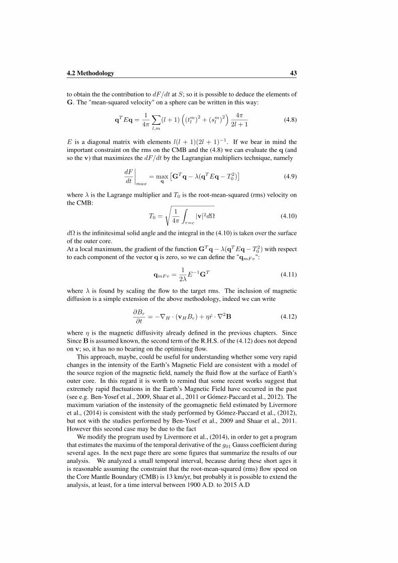
to obtain the the contribution to dF/dt at S; so it is possible to deduce the elements ofG. The "mean-squared velocity" on a sphere can be written in this way:
qT Eq =
14π
l,m
(l + 1)(tm
l)2 + (sm
l)2
4π
2l + 1(4.8)
E is a diagonal matrix with elements l(l + 1)(2l + 1)−1. If we bear in mind theimportant constraint on the rms on the CMB and the (4.8) we can evaluate the q (andso the v) that maximizes the dF/dt by the Lagrangian multipliers technique, namely
dF
dt
max
= maxq
G
Tq− λ(qT Eq− T 2
0 )
(4.9)
where λ is the Lagrange multiplier and T0 is the root-mean-squared (rms) velocity onthe CMB:
T0 =
14π
r=c
|v|2dΩ (4.10)
dΩ is the infinitesimal solid angle and the integral in the (4.10) is taken over the surfaceof the outer core.At a local maximum, the gradient of the function G
Tq− λ(qT Eq− T 2
0 ) with respectto each component of the vector q is zero, so we can define the "qmFv":
qmFv =12λ
E−1G
T (4.11)
where λ is found by scaling the flow to the target rms. The inclusion of magneticdiffusion is a simple extension of the above methodology, indeed we can write
∂Br
∂t= −∇H · (vHBr) + ηr ·∇2
B (4.12)
where η is the magnetic diffusivity already defined in the previous chapters. SinceSince B is assumed known, the second term of the R.H.S. of the (4.12) does not dependon v; so, it has no no bearing on the optimising flow.
This approach, maybe, could be useful for understanding whether some very rapidchanges in the intensity of the Earth’s Magnetic Field are consistent with a model ofthe source region of the magnetic field, namely the fluid flow at the surface of Earth’souter core. In this regard it is worth to remind that some recent works suggest thatextremely rapid fluctuations in the Earth’s Magnetic Field have occurred in the past(see e.g. Ben-Yosef et al., 2009, Shaar et al., 2011 or Gómez-Paccard et al., 2012). Themaximum variation of the instensity of the geomagnetic field estimated by Livermoreet al., (2014) is consistent with the study performed by Gómez-Paccard et al., (2012),but not with the studies performed by Ben-Yosef et al., 2009 and Shaar et al., 2011.However this second case may be due to the fact
We modify the program used by Livermore et al., (2014), in order to get a programthat estimates the maximu of the temporal derivative of the g01 Gauss coefficient duringseveral ages. In the next page there are some figures that summarize the results of ouranalysis. We analyzed a small temporal interval, because during these short ages itis reasonable assuming the constraint that the root-mean-squared (rms) flow speed onthe Core Mantle Boundary (CMB) is 13 km/yr, but probably it is possible to extend theanalysis, at least, for a time interval between 1900 A.D. to 2015 A.D
44 4. Outer Core Dynamics and rapid intensity changes
1980 1985 1990 1995 2000 2005 2010 2015
120.5
121.0
121.5
122.0
122.5
t !years"
Max#d
g10
dt$
! nT%y"
Figure 4.1: Maximum temporal variation of g01 in the ages between 1980 A.D. and 2015 A.D.(these coefficients are by IGRF12 model (Thebault et al., 2015))
4.2 Methodology 45
1980 1982 1984 1986 1988 1990
121.8
122.0
122.2
122.4
t !years"
Max#d
g10
dt$
! nT%y"
Figure 4.2: Maximum temporal variation of g01 in the ages between 1980 A.D. and 1990 A.D.(these coefficients are by CALS10k model (Korte et al., 2011))
46 4. Outer Core Dynamics and rapid intensity changes
1980 1982 1984 1986 1988 1990
121.8
122.0
122.2
122.4
t !years"
Max#d
g10
dt$
! nT%y"
Figure 4.3: Maximum temporal variation of g01 in the ages between 1980 A.D. and 1990 A.D.(these coefficients are by CALS3k model (For reference about this modelKorte andConstable, 2003 and Korte et al., 2009))
Chapter 5
Discussion and Conclusions
In this thesis we deal with some aspects of the Dynamo Theories. In the Chapter 3,we looked for a connection between the recent trend of the geomagnetic field and theturbulent dynamo theories. The models of the geomagnetic field of the last 3000, 7000,10000 and 14000 years show a field that has intermittent decays so that the magneticdiffusivity would correspond to a value of conductivity much smaller than the mostcommonly accepted value. If we compare Figs. 3.1, 3.3 and 3.4, we can see that thereis no contemporary turbulent diffusive behaviour in the different studied models; in factthe exponential decays of the dipole field occur in different epochs for different models.However, as we can check by the tables 3.1, 3.2 and 3.3, almost all apparent electricalconductivities are one order of magnitude smaller than the commonly accepted values,that are probably more correct than ours. In other words, all models show that whenthe geomagnetic dipolar field decays it does with a rate faster than the typical diffusiverate so we can speculate that this is a general feature of the geomagnetic field of thelast millennia. This is due to the presence of an additional term β in the diffusion part(see eq.(3.8)), so we can call this process a "turbulent diffusive" regime of the recentgeomagnetic field. This "turbulent diffusivity" is probably due to the turbulence effectsin the core and accelerates the process of field decay (according to the (3.8)). This tur-bulent diffusivity would explain why our conductivity values, obtained neglecting theinductive term in (3.1), are one order of magnitude smaller than the expected values forthe core. In this regard, we recall that 5 × 10⁵ S/m, a value we find quite often in theliterature (see e.g. Gubbins and Roberts, 1987 and also Stacey and Anderson, 2001)and 2.76 × 10⁵ S/m (that is a more recent estimate performed by Stacey and Loper,2007), are approximately one order of magnitude greater than our σi. This turbulentdiffusivity, in turn, could eventually bring the planetary magnetic field toward a fieldreversal in a sort of avalanche process, typical of a turbulent, and occasionaly chaotic,regime. This turbulent diffusive effect, as we will see in the Appendix A, is greater incase of a isotropic, homogeneous and mirror-symmetric turbulence. This is coherentwith some other papers (see for example De Santis, 2007 or Hulot et al., 2002, whichare based on fully different approaches) that suggest that an imminent magnetic fieldreversal is possible (about 1000 or 2000 years from now). Also the article of Liu andOlson (2009) could support our hypothesis; in fact it reminds the very fast decrease ofthe geomagnetic dipole moment in the last 160 years (at least one order of magnitudefaster than the free decay rate) and emphasizes that the process of advective mixing inthe core can enhance the magnetic diffusion. There are also other articles that show thatthe geomagnetic dipole moment has recently decayed with a rate faster than the typical
48 5. Discussion and Conclusions
diffusive rate (see e.g. Gubbins et al., 2006 and other references here cited). Howevermost of this works speak about the last century or the last 4 centuries. Instead, ourresults show a turbulent diffusive regime regime which lasts for at least 14000 years.This, in our opinion, strengthens the hypothesis that the recent geomagnetic field is ina turbulent diffusive regime. Furthermore, there is a paleomagnetic study described inNowaczyk et al. (2012) that shows that the Laschamp excursion occurred in a timemuch shorter than the time corresponding to the free decay rate due to the ohmic diffu-sion of the geomagnetic field. In fact the record relating to this excursion, shows a fullpolarity reversal, although temporary, that lasted for about 200 years; the whole pro-cess, namely from the beginning when there was the current geomagnetic polarity untilthe end, when there was again the current geomagnetic polarity, lasted for about 3600years, a time comparable to the relaxation times estimated by us from the geomagneticglobal models. Therefore, an excursion, and so probably also a polarity reversal, wouldoccur in a time faster than the time corresponding the typical magnetic diffusivity. Thisexperimental observation could suggest that before an excursion or reversal there is aturbulent diffusive regime. For some details about the Laschamp excursion see the ar-ticle of Nowaczyk et al. (2012). Of course, because of the limited number of caseshere analysed, further studies will be necessary to establish if the hypothesis of theturbulent diffusivity for the recent geomagnetic field is correct or not. This could beverified in several ways. For instance, we could try to estimate some other importantgeophysical parameters such as, for example, the β coefficient in the eq. (3.8). Infact, as it is shown in the Appendix A, this coefficient is connected with |v|2. In otherwords we could do some more accurate estimations of other important parameters, oruse some values reported in other woks, to try to solve the magnetic induction equationunder less restrictive assumptions and then compare the results with those of previousworks (e.g. with the Glatzmaier-Roberts dynamo described in Glatzmaier and Roberts(1995a; 1995b)) and with experimental data. More specifically, it will be worth tryingto solve the (3.9) or more simplified expressions (for example we can assume that |v|2is uniform and constant or that c(00) a(00) and c(00) a(01)). Furthermore we couldtry to estimate the terms O(|v|3) or O(|v|4) of ∆ (for more details see the AppendixA). In this manner we may find a solution of the magnetic field less approximate thanthe solution of the diffusive part of the (3.1) and we can, by simple numerical simu-lations, compare these results with experimental data. Moreover we could repeat ouranalyses on some regional models; so we can verify if there are some turbulent diffu-sive behaviours limited to more restricted regions. This would be important becausethere are some regions where the geomagnetic field decays more quickly than in othersand there also some regions where it seems that the magnetic field doesn’t decay at all(Gubbins, 1987). So we could try to understand if the turbulent diffusivity is also spacedependent.
There are several arguments that suggest that the turbulent diffusivity may be animportant component of any possible magnetic field reversal. In fact if the inductiveterm disappears, the decay times will be about 10000 years instead of about 1000-2000years as it reported in several papers (see e.g. Liu and Olson, 2009 or Hulot et al.,2002). But if the inductive term vanishes, maybe the magnetic field will not regener-ate itself. So we think that a better understanding of the turbulence in the core can beuseful to improve our knowledge about the generation, extinction and regeneration ofthe geomagnetic field. On the other hand, several authors believe that the geomagneticpolarity reversal might be connected with a magnetic flux of opposite sign in the south-ern hemisphere (see e.g. Gubbins, 1987); so we could try to compare these types ofstudies with our studies on the turbulent diffusivity of the geomagnetic field. Another
49
interesting aspect of the dynamo theories is the role of the symmetries as explained forexample in Rädler (1968a) or in Merrill et al. (1996). We think that these studies couldbe useful to understand better some aspects of the dynamics of the Earth’s MagneticField, that has several features not well-understood yet.It is interesting to note, by analyzing the Figures 4.1, 4.2 and 4.3 that when the dipolargeomagnetic field exponentially decay its temporal derivative linearly decrease. Maybeit could be interesting to do other analysis with simulations or during real situations, inorder to check whether this feature is verified before a polarity reversal or excursion.
50 5. Discussion and Conclusions
Appendix A
Calculation of the meanelectromotive force
In this appendix we will give some details on the calculation of the mean electromotiveforce within suitable approximations. We will perform some manipulations in a sim-ilar way as was already done by different authors (see Moffatt, 1978; Rädler, 1968a;1968b).
To discuss the term ∆ in (3.6) and (3.7) we need, at least, a formal solution of the(3.7); so we assume that V = V0, v, B0 = B and (for the moment) C are known andwe rewrite the (3.7) in tensor notation 1
η∇2bi + εimnεnpq
∂
∂xm
V pbq
− ∂bi
∂t= −εimn
∂
∂xm
εnpqvpBq + Cn) (A.1)
We may solve (A.1) with a suitable boundary condition on b(r, t0) in the form
bi(r, t) =
Gil(r, t; r, t0)bl(r, t0)dr+
+
t
t0
Gil(r, t; r, t)εlmn
∂
∂xm
εnpqvp(r, t)Bq(r, t) + Cn(r, t)
drdt
(A.2)where Gil(r, t; r, t) is a suitable function that satisfies the following properties
dr in the (A.2), are, of course, integrals that must
1In this appendix we adopt the Einstein summation convention everytime we write two repeated indicesand do not use the symbol of sum
P
52 A Calculation of the mean electromotive force
be taken over all the space. Now we set bi(r, t0) = 0 ∀ i and, for semplicity we supposethat V0 = 0. With this condition Gil is the following well-known Green’s function
Gil(r, t; r, t) = δil
1
η4π(t− t)
3/2
exp− |r− r
|24η(t− t)
With the condition bi(r, t0) = 0 ∀ i, after an integration by parts and other simple stepswe obtain
We can also write a more general expressions for ∆i
∆i =
t
t0
Kiq(r, t; r, t)Bq(r, t)drdt (A.7)
where Kiq(r, t; r, t) can be deduced from (A.6) and (A.2). Now we suppose that thecorrelation tensors, namely the expressions vj(r, t)vp(r, t), vj(r, t)vj(r, t)vp(r, t)and the other averages of higher order in vi, differ significantly from zero only for smallvalues of |r − r
| and t − t; this is a reasonable approximation because, as we havealready said, the turbulence phenomena are bounded in a small region and in time-scalemuch smaller than T ; we therefore need only to know Bq(r, t) in a small neighbour-hood of r
= r and t = t; so after a Taylor expansion of Bq(r, t) we can write
∆i = g(00)iq
Bq(r, t) +
k+ν≥1
g(kν)iqr...s
∂k+νBq(r, t)∂xr...∂xs∂tν
(A.8)
where k is the space-derivative order, ν is the time-derivative order and g(00)iq
So the main problem in the mean-field dynamo theory is to determine the correlationtensors. In the next pages we will give some details about this question (Rädler, 1968b).If we replace the integration variables r
and t by Ξ ≡ r−r and τ ≡ t−t respectively
we can rewrite the (A.9) in this manner
g(kν)iqr...s
= εijkεkmnεnpq
(−1)k+ν
k!ν!
t
t0
1Ξ
∂G(Ξ, τ)∂Ξ
·
·Rjp(r, t;−ξ,−τ )ΞmΞr...ΞsτνdΞdτ + O(|v|3) (A.10)
53
where Ξ = |Ξ|,
G(ξ, τ) =
1η4πτ
3/2
exp− Ξ2
4ητ
andRjp(r, t;Ξ, τ) = vj(r, t)vp(r + Ξ, t + τ)
It can be shown (see for example Rädler, 1968b) that within suitable approximations
where f0, g0, f1, g1, h1 and k1 are suitable functions that depend on the geometry andon the dynamics of the Earth’s outer core; the first three terms of the (A.11) (involv-ing f0 and g0) give the correlation tensor in the homogeneous, isotropic and mirror-symmetric case, while the remainder, involving ∇|v|2, described departures from thatstate.
We are mainly interested, as we will explain better later, only in a few terms of theexpression (A.8) so we write
∆i ≈ g(00)iq
Bq(r, t) + g(10)iqr
∂Bq(r, t)∂xr
+ g(01)iq
∂Bq(r, t)∂t
(A.12)
If we retain only O(|v|2) terms in the (A.9), bearing in mind the (A.11), we can easilydeduce from the (A.10) that
g(10)iqr
= εiqr
13|v|2(r, t)c(00) (A.13)
g(0ν)iq
= εiqj
(−1)ν
3ν!∂|v|2∂xj
(r, t)a(0ν) (A.14)
with
c(00) = −4π
3
t
t0
∂G(Ξ, τ)∂Ξ
f0(t; Ξ,−τ)Ξ3dΞdτ
and
a(0ν) = −4π
3
t
t0
∂G(Ξ, τ)∂Ξ
[f1(t; Ξ,−τ)+ g1(t; Ξ,−τ)+ k1(t; Ξ,−τ)]Ξ3τνdΞdτ
and in some situations c(00) is positive (see for example Rädler, 1968b) so if we sub-stitute (A.13) and (A.12) in (3.6) we obtain the equation (3.8)
∂B0
∂t= ∇× (V0 ×B0) + (η + β)∇2
B0 + ... (3.8)
54 A Calculation of the mean electromotive force
It is worth to note that if we assume a homogeneous, isotropic and mirror-symmetricturbulence the term g(0ν)
iq= 0 (see the comment under (A.11)); so in this situation if
we look at the (3.6) at the lowest orders we find only the turbulent diffusive term andwe do not find any terms derived by (A.14); in other words if there is a homogeneous,isotropic and mirror-symmetric turbulence the process of field decay is further acceler-ated and, consequently, the chance for a magnetic polarity reversal is even greater. Asanticipated at the end of the section 3.1, we can consider a more particular expressionof the (3.8) substituting (A.12), (A.13) and (A.14) in (3.6) and assuming V0 = 0
∂Bi
∂t= (η +
13|v|2c(00))∇2Bi +
c(00)
3
∂|v|2∂xj
∂Bi
∂xj
− ∂|v|2∂xj
∂Bj
∂xi
+
+a(00)
3
Bi∇2|v|2 +
∂Bi
∂xj
∂|v|2∂xj
−Bj
∂2|v|2∂xj∂xi
+
+a(01)
3
∂2|v|2∂xj∂xi
∂Bj
∂t−∇2|v|2 ∂Bi
∂t− ∂|v|2
∂xj
∂2Bi
∂xj∂t
+ ... (3.9)
Other useful references on the calculation of the correlation tensor and on his impor-tance in the dynamo theories in turbulent conditions can be found in the book of Krauseand Rädler, (1980) and in the article of Rädler (1974).
Bibliography
Abramowitz, M. and I.A. Stegun, Handbook of mathematical functions, 1046 pp., Dover Publications, NewYork, 1970.
Backus, G.E., R. Parker and C. Constable, Foundations of Geomagnetism, Cambridge University Press,Cambridge, 1996.
Baranger, M., Chaos, Complexity and Entropy: a Physics Talk for Non-Physicists, Wesleyan UniversityPhysics Dept. Colloquium, 2001.
Ben-Yosef, E.,L. Tauxe, T.E. Levy, R. Shaar, H. Ron and M. Najjar, Geomagnetic intensity spike recordedin high resolution slag deposit in Southern Jordan, Earth Planet. Sci. Lett., 287, 529–539, 2009.
Constable, C.G. and M. Korte, Is the Earth’s magnetic field reversing?, Earth Planet. Sci. Lett., 246, 1–16,2006.
Constable, C.G. and R. L. Parker, Statistics of theGeomagnetic Secular Variation for the Past 5 m.y., J.Geophys. Res., 93, 11569–11581, 1988.
De Santis, A., D.R. Barraclough and R. Tozzi, Spatial and temporal spectra of the geomagnetic field andtheir scaling properties, Phys. Earth Planet. Inter. 135, 125–134, 2003.
De Santis, A., R. Tozzi and L.R. Gaya-Piqué, Information content and K-Entropy of the present geomagneticfield, Earth Planet. Sci. Lett., 218, 269–275, 2004.
De Santis, A., How persistent is the present trend of the geomagnetic field to decay and, possibly, to reverse?,Phys. Earth Planet. Inter., 162, 217–226, 2007.
De Santis, A., Geosystemics, 3rd WSEAS International Conference on Geology and Seismology, Cambridge,36–40, 2009.
De Santis A. and E. Qamili, Shannon information of the geomagnetic field for the past 7000 years, NonlinearProc. Geophys., 17, 77–84, 2010.
De Santis et al., Geomagnetic Field Modelling, CSES-Limadou Mission, ASI–Aula Cassini, 2016.
Dziewonski, A. M. and D. L. Anderson Preliminary reference Earth model, Phys. Earth Planet. Inter., 25,297–356, 1981.
Filippi, E., A. De Santis, F.J. Pavón-Carrasco, B. Duka and K. Peqini, Some evidence for a TurbulentDiffusion in the Geodynamo from geomagnetic global models of the last few millennia, 26th IUGGGeneral Assembly, Prague, 2015(available at https://drive.google.com/file/d/0B-vFmSm_gnQfNFhTcTRrUEVXbHM/view?pref=2&pli=1)
Finlay, C. C., S. Maus, C. D. Beggan, T. N. Bondar, A. Chambodut, T. A. Chernova, A. Chulliat, V. P.Golovkov, B. Hamilton, M. Hamoudi, R. Holme, G. Hulot, W. Kuang, B. Langlais, V. Lesur, F. J. Lowes,H. Lühr, S. Macmillan, M. Mandea, S. McLean, C. Manoj, M. Menvielle, I. Michaelis, N. Olsen, J.Rauberg, M. Rother, T. J. Sabaka, A. Tangborn, L. Tøffner-Clausen, E. Thébault, A. W. P. Thomson, I.Wardinski, Z. Wei and T. I. Zvereva, International Geomagnetic Reference Field: the eleventh generation,Geophys. J. Int., 183, 1216–1230, 2010.
56 BIBLIOGRAPHY
Ganguly, J., Thermodynamics in Earth and Planetary Sciences, Springer, 2009.
Glatzmaier, G.A. and P.H. Roberts, A three-dimensional convective dynamo solution with rotating andfinitely conducting inner core and mantle, Phys. Earth Planet. Inter., 91, 63–75, 1995a.
Glatzmaier, G.A. and P.H. Roberts, A three-dimensional self-consistent computer simulation of a geomag-netic field reversal, Nature, 377, 203–209, 1995b.
Gómez-Paccard, M., A. Chauvin, P. Lanos, P. Dufresne, M. Kovacheva, M.J. Hill, E. Beamud, S. Blain, A.Bouvier and P. Guibert, Archaeological Working Team, Improving our knowledge of rapid geomagneticfield intensity changes observed in Europe between 200 and 1400 AD, Earth Planet. Sci. Lett., 355,131–143, 2012.
Gruzinov, A.V. and P.H. Diamond, Self-Consistent Theory of Mean-Field Electrodynamics, Phys. Rev. Let-ters, 72, 1651–1653, 1994.
Gubbins, D., Mechanism for geomagnetic polarity reversals, Nature, 362, 167–169, 1987.
Gubbins, D. and P.H. Roberts, Magnetohydrodynamics of the Earth Core, in Geomagnetism 2, Edited by J.A. Jacobs, 579 pp., Academic Press, London, 1987.
Gubbins, D., A.L. Jones and C.C. Finlay Fall in Earth’s Magnetic Field is Erratic, Science, 312, 900–902,2006.
Heller, P. Experimental investigations of critical phenomena, Rep. Prog. Phys., 30, 731–826, 1967.
Holme, R., Large-scale flow in the core, in Olson, P. (Ed.), in Treatise on Geophysics, 8, Elsevier, 107–130,2007.
Hulot, G., C. Eymin, B. Langlais, M. Mandea and N. Olsen, Small-scale structure of the geodynamo inferredfrom Oersted and Magsat satellite data, Nature, 416, 620–623, 2002.
Kolel-Veetil, M.K. and T.K. Keller Organometallic Routes into the Nanorealms of Binary Fe-Si Phases,Materials, 3, 1049–1088, 2010.
Korte, M. and C.G. Constable, Continuous global geomagnetic field models for the past 3000 years, Phys.Earth Planet. Inter., 140, 73–89, 2003.
Korte, M. and C.G. Constable, Continuous Geomagnetic Field Models for the Past 7 Millennia: 2.CALS7k,Geochem. Geophy. Geosy., 6, Q02H16, doi:10.1029/2004GC000801, 2005.
Korte, M., F. Donadini and C.G. Constable, Geomagnetic field for 0-3 ka: 2. A new series of time-varyingglobal models, Geochem. Geophy. Geosy., 10, Q06008, doi:10.1029/2008GC002297, 2009.
Korte, M., C. Constable, F. Donadini and R. Holme, Reconstructing the Holocene geomagnetic field, EarthPlanet. Sci. Lett., 312, 497–505, 2011.
Krause, F. and K.H. Rädler, Mean-Field Magnetohydrodynamics and Dynamo Theory, 271 pp., Akademie-Verlag, Berlin, 1980.
Leprovost, N. and E-J. Kim, Self-Consistent Mean Field Theory In Weakly Ionized Media, The Astroph.Journ., 598, L99–L102, 2003.
Liu, L. and P. Olson, Geomagnetic dipole moment collapse by convective mixing in the core, Geophys. Res.Lett., 36, L10305, doi:10.1029/2009GL038130, 2009.
Livermore, P.W., A. Fournier and Y. Gallet, Core-flow constraints on extreme archeomagnetic intensitychanges, Earth Planet. Sci. Lett., 387, 145–156, 2014.
Maus, S., S. Macmillan, T. Chernova, S. Choi, D. Dater, V. Golovkov, V. Lesur, F. Lowes, H. Lühr, W.Mai, S. McLean, N. Olsen, M. Rother, T. Sabaka, A. Thomson and T. Zvereva, The 10th GenerationInternational Geomagnetic Reference Field, Phys. Earth Planet. Inter., 151, 320–322, 2005a.
Maus, S., S. Macmillan, T. Chernova, S. Choi, D. Dater, V. Golovkov, V. Lesur, F. Lowes, H. Lühr, W.Mai, S. McLean, N. Olsen, M. Rother, T. Sabaka, A. Thomson and T. Zvereva, The 10th-GenerationInternational Geomagnetic Reference Field, Geophys. J. Int., 161, 561–565, 2005b.
BIBLIOGRAPHY 57
Merrill, R.T., M.W. McElhinny and P.L. McFadden, The Magnetic Field of the Earth, 531 pp., AcademicPress, San Diego, 1996.
Moffatt, H.K., Magnetic Field Generation in Electrically Conducting Fluids, 343 pp., Cambridge UniversityPress, Cambridge, 1978.
Nilsson, N., R. Holme, M. Korte, N.Suttie and M. Hill, Reconstructing Holocene geomagnetic field variation:new methods, models and implications, Geophys. J. Int., 198, 229–248, 2014.
Nowaczyk, N.R., H.W. Arz, H.W. Frank, J. Kind and B. Plessen, Dynamics of the Laschamp geomagneticexcursion from Black Sea sediments, Earth Planet. Sci. Lett., 351-352, 54–69, 2012.
Pan, Y., R. Zhu, S.K. Banerjee, J. Gill, Q. Williams, Rock magnetic properties related to thermal treatmentof siderite: Behavior and interpretation, J. Geophys. Res., 105, 783–794, 2000.
Parker, R.L., Notes on Geomagnetism, (available at http://igppweb.ucsd.edu/~parker/SIO229/index.html),2005.
Pavón-Carrasco, F.J., M.L. Osete, J.M. Torta and A. De Santis, A geomagnetic field model for the Holocenebased on archaeomagnetic and lava flow data, Earth Planet. Sci. Lett., 388, 98–109, 2014.
Pozzo, M., C. Davies, D. Gubbins and D. Alfè, Thermal and electrical conductivity of iron at Earth’s coreconditions, Nature, 485, 355–358, doi:10.1038/nature11031, 2012.
Rädler, K.H., On the Electrodynamics of Conducting Fluids in Turbulent Motion, I. The Principles of MeanField Electrodynamics, Z. Naturforsch., 23a, 1841–1851, 1968a. [English translation: Roberts and Stix,1971 pp. 247–265].
Rädler, K.H., On the Electrodynamics of Conducting Fluids in Turbulent Motion, II. Turbulent Conductivityand Turbulent Permeability, Z. Naturforsch., 23a, 1851–1860, 1968b. [English translation: Roberts andStix, 1971, pp. 267–289].
Rädler, K.H., On the Influence of a Large-scale Magnetic Field on Turbulent Motions in an ElectricallyConducting Medium, Astron. Nachr., 295, 265–273, 1974.
Roberts, P.H. and M. Stix, The Turbulent Dynamo: a Translation of a Series of Papers byKrause, F., Rädler, K.H., Steenbeck, M., NCAR Technical Note TN-60, June, 1971 (available athttp://nldr.library.ucar.edu/repository/collections/TECH-NOTE-000-000-000-045).
Ruetsch, G.R.and M.R. Maxey, Small-scale features of vorticity and passive scalar fields in homogeneousfluids, Phys. Fluids A, 3, 1587–1597, 1991.
Shaar, R., E. Ben-Yosef, H. Ron, L. Tauxe, A. Agnon and R. Kessel, Geomagnetic field intensity: How highcan it get? How fast can it change? Constraints from Iron Age copper slag, Earth Planet. Sci. Lett., 301,297–306, 2011.
Stacey, F.D. and O.L. Anderson, Electrical and thermal conductivities of Fe-Ni-Si alloy under core condi-tions, Phys. Earth Planet. Inter., 124, 153–162, 2001.
Stacey, F.D. and D.E. Loper, A revised estimate of the conductivity of iron alloy at high pressure and impli-cations for the core energy balance, Phys. Earth Planet. Inter., 161, 13–18, 2007.
Thébault, E. et al., International Geomagnetic Reference Field: the 12th generation, Earth, Planets andSpace, doi:10.1186/s40623-015-0228-9, 2015.
Yukutake, T., Free Decay of Non-Dipole Components of the Geomagnetic Field, Phys. Earth Planet. Inter.,1, 93–96, 1968.