57
Geoid modelling with GRAVSOFT Rene Forsberg, DTU-Space, Denmark

Geoid modelling with GRAVSOFT Rene Forsberg, DTU-Space, Denmark

Heights from GPS: H = hellipsoidal – N The 1 cm-geoid is within reach in countries with good gravity coverage or for special projects like large bridges ..
The geoid use
Marine areas: MDT = MSS – N MSS: mean sea surface (Altimetry or GPS) Several ”geoids” in prac- tical use, need for improved datums

Anomalous potential T = Wphysical – Unormal The anomalous gravity potential T is split into 3 parts:
T = TEGM + TRTM + Tres
TEGM – Global spherical harmonic model (EGM08/GOCE to degree 360 or
2190) TRTM – residual terrain effect (RTM) .. Computed by prism integration Tres – residual (i.e. unmodelled) local gravity effect Principle used much in gravimetric geoid determination: “remove-restore” Stokes function usually implemented by Fast Fourier Techniques and/or least-squares collocation
);( geoidonTNγ
=
Geoid determination
σψπγ
ζσ
d ) S()g+g( 4
R = 1∆∫∫
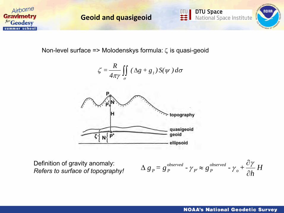
Non-level surface => Molodenskys formula: ζ is quasi-geoid
Definition of gravity anomaly: Refers to surface of topography! H
h + -g -g = g o
observedPP
observedPP ∂
∂≈∆ ′
γγγ
Geoid and quasigeoid

Hl/m]0.1543[mga -C C = H
l/m]H0.0424[mga +gC
gC = H
*o
*
PHelmert
γγ≈
≈
H g - Hl/m]H0.1967[mga + - g - H -H = N -
o
B
o
oP*PP γγ
γζ∆
≈⋅≈
Normal and orthometric (Helmert) heights <-> quasigeoid and geoid
Normal heights: quasigeoid Orthometric heights: geoid Theoretical problem: Density of Earth must be known to define geoid - ”New Theory” approx. 1960 by Molodensky
Height systems

Integral Formulas – space domain
∫∫∆==
σ
σψπ
γ dgSRNT )(4
Stokes Formula • Relating N with gravity observations.
• Stokes Kernel
• w is weight function … used to limit influence of low harmonics
ϕϕλλϕϕψ
ψψψψψψ
ψψ
coscos2
)(sin
2)(
sin2
sin
)2
sin2
ln(sincos3cos512
sin6)2/sin(
1
)(cos112)(
222
2
21
ppp
lPwllS
−+
−=
+−−+−
=−+
= ∑∞
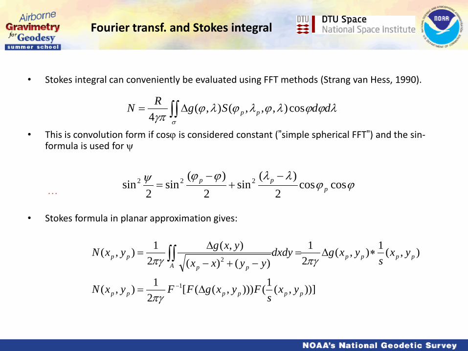
Fourier transf. and Stokes integral
• Stokes integral can conveniently be evaluated using FFT methods (Strang van Hess, 1990).
• This is convolution form if cosϕ is considered constant (”simple spherical FFT”) and the sin-formula is used for ψ …
• Stokes formula in planar approximation gives:
∫∫ ∆=σ
λϕϕλϕλϕλϕγπ
ddSgRN pp cos),,,(),(4
))],(1())),(([2
1),(
),(1),(2
1)()(
),(2
1),(
1
2
pppppp
ppppA pp
pp
yxs
FyxgFFyxN
yxs
yxgdxdyyyxx
yxgyxN
∆=
∗∆=−+−
∆=
−
∫∫
πγ
πγπγ
ϕϕλλϕϕψ coscos
2)(
sin2
)(sin
2sin 222
ppp −
+−
=

sin2 ψ2
≈ sin2 ϕp − ϕ2
+ sin2 λ p − λ2
cosϕ ι cos[ϕ ι − (ϕ ι − ϕ)]
≈ sin2 ϕ p − ϕ2
+ sin2 λ p − λ2
[cos 2 ϕ ι cos(ϕ ι − ϕ ) + cosϕ ι sinϕ ι sin(ϕ ι − ϕ )]
Improved method: bandwise FFT
Method is exact along borders between bands, linear interpolation in between (Forsberg and Sideris, 1987)
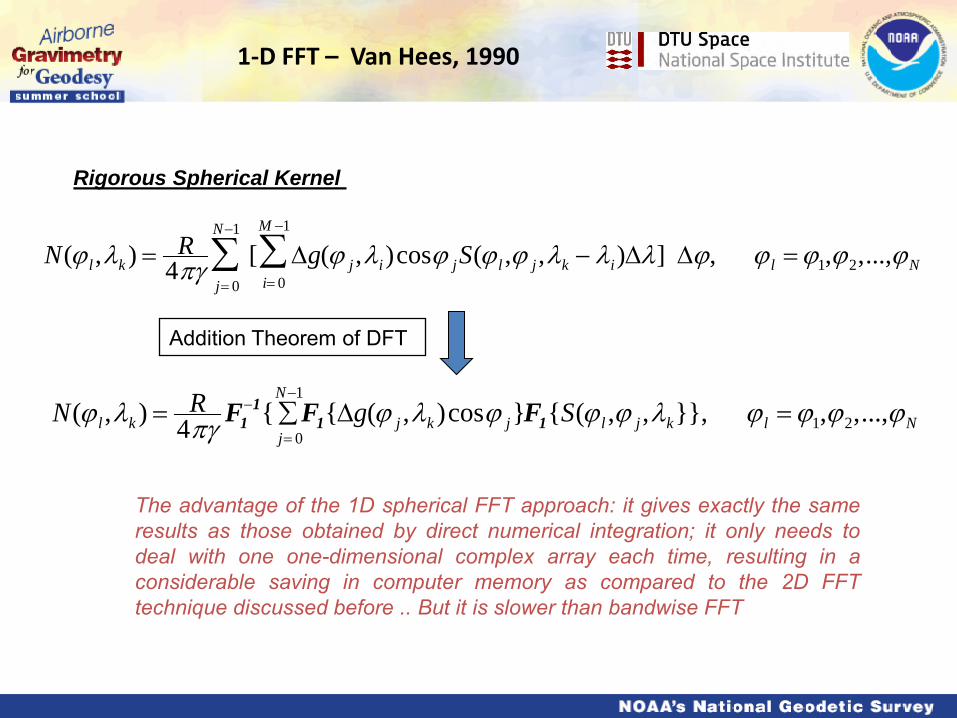
1-D FFT – Van Hees, 1990
Rigorous Spherical Kernel
N(ϕ l ,λk ) = R4πγ [ ∆
i= 0
M −1
∑j= 0
N−1
∑ g(ϕ j ,λi)cosϕ jS(ϕ l ,ϕ j ,λk − λi)∆λ] ∆ϕ, ϕ l = ϕ1,ϕ2,...,ϕN
Addition Theorem of DFT
N(ϕ l ,λk ) = R4πγ F1
−1{ F1{∆g(ϕ j ,λk )cosϕ j}j= 0
N−1∑ F1{S(ϕ l ,ϕ j ,λk}}, ϕ l = ϕ1,ϕ2,...,ϕN
The advantage of the 1D spherical FFT approach: it gives exactly the same results as those obtained by direct numerical integration; it only needs to deal with one one-dimensional complex array each time, resulting in a considerable saving in computer memory as compared to the 2D FFT technique discussed before .. But it is slower than bandwise FFT

Modified kernels needed
Takes into account the influence of possible (likely!) terrestrial+airborne biases
0
200
400
1 2 3 4
Mod 360Mod 60Mod 30
s (degrees)
S'(s
)Wong-Gore modified Stokes function
Choice of degree of modification for GOCE still an open problem! (requires good GPS-levelling)
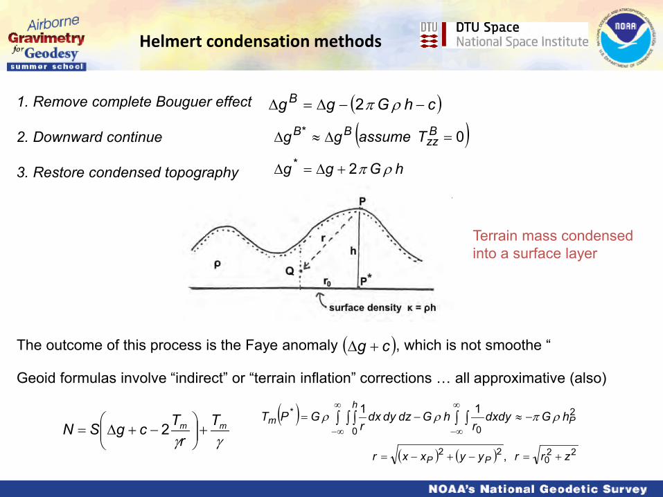
Helmert condensation methods 1. Remove complete Bouguer effect 2. Downward continue 3. Restore condensed topography
The outcome of this process is the Faye anomaly , which is not smoothe “ Geoid formulas involve “indirect” or “terrain inflation” corrections … all approximative (also)
( )chGggB −−∆=∆ ρπ2
( )0* =∆≈∆ Bzz
BB Tassumegg
hGgg ρπ2* +∆=∆
( )cg +∆
Terrain mass condensed into a surface layer
γγmm T
rTcgSN +
−+∆= 2
( ) ∫ ∫ ∫ ∫ ∫∞
∞−
∞
∞−−≈−=
hPm hGdxdy
rhGdzdydx
rGPT
0
2
0
* 11 ρπρρ
( ) ( ) 220
22 , zrryyxxr PP +=−+−=

Nordic geoid example
NKG geoids: Denmark,Sweden, Norway, Finland, Estonia, Latvia, Lithuania .. Joint geoid Next: NKG-2015 – goal: 1 cm geoid (2 cm in the mountains), airborne gravity fill-in (yellow)

Data reduction: GOCE R5+EGM08 composite model / terrain effects GRAVSOFT: HARMEXP, TC and SPFOUR
Free-air gravity Data
Land gravity
(434925)
Airborne gravity (17238)
Original Mean
1.0
-8.7
Std.dev. 25.2 23.3
-GOCE/EGM Mean
-1.1
1.2
Std.dev. 16.0 15.4
-RTM effect Mean
0.3
1.3
Std.dev. 10.8 15.4
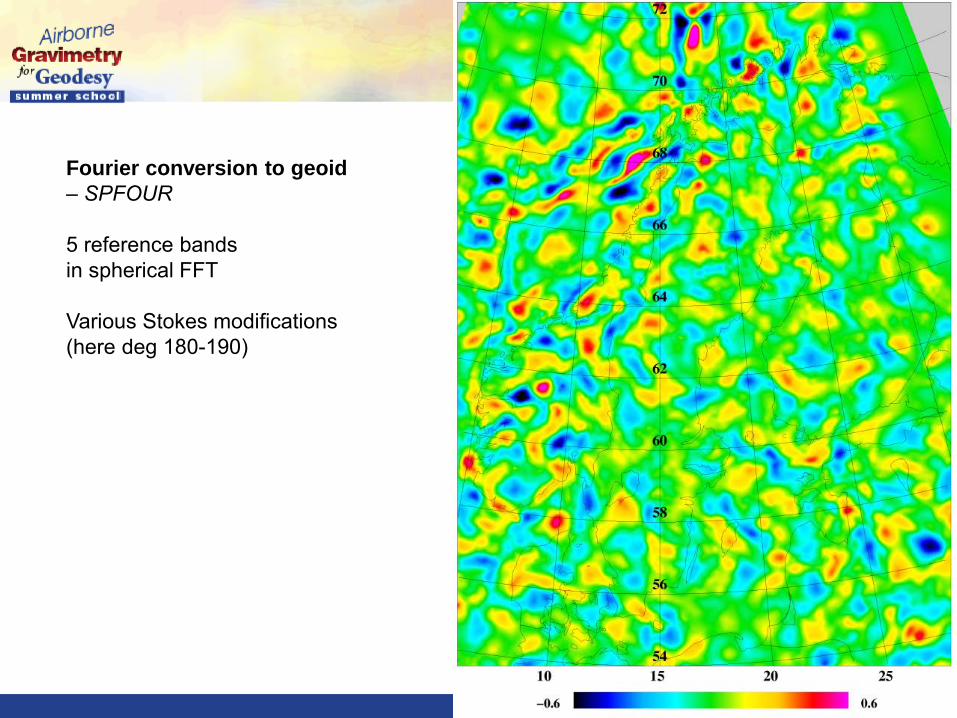
Fourier conversion to geoid – SPFOUR 5 reference bands in spherical FFT Various Stokes modifications (here deg 180-190)

Terrain effects Computed by FFT
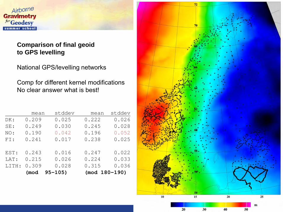
Comparison of final geoid to GPS levelling National GPS/levelling networks Comp for different kernel modifications No clear answer what is best!
mean stddev mean stddev DK: 0.209 0.025 0.222 0.026 SE: 0.249 0.030 0.245 0.028 NO: 0.190 0.042 0.196 0.052 FI: 0.241 0.017 0.238 0.025 EST: 0.243 0.016 0.247 0.022 LAT: 0.215 0.026 0.224 0.033 LITH: 0.309 0.028 0.315 0.036 (mod 95-105) (mod 180-190)

Gravity anomalies – Fehmarn Belt tunnel project Land, marine and airborne (DTU/BKG - COWI acft)
Fehmarn Belt link
Germany
Denmark

Difference DTU-BKG geoid
Operational geoid <1 cm to fixed link (tunnel project) … common elevation reference
Geoid connections across Fehmarn Belt

Geoid fits to GPS – Denmark
Fitted to DVR90 – 3rd national levelling (with geoid used for datum on small islands)
REFDK – national 10 km GPS net Geoid correction signal: - Bornholm in own datum - Small islands in geoid-determined datum

Geoid data – Unit m
All GPS except small islands (677 pts)
Bornholm (20 pts)
Mean Std.dev. Mean Std.dev.
NKG04 geoid -0.004 0.027 0.107 0.158
EGM2008 0.298 0.026 0.439 0.016
DKGEOID (GOCE mod. degree 150-160)
0.288 0.021 0.414 0.013
Fitted geoid 0.000 0.006 0.001 0.006
Denmark geoid compared to GPS
•The 1-cm geoid is available – used externsively • Current challenges: marine geoid … how to fit?

(EU Interreg project BLAST – Bringing Land And Sea Together)
Geoid (with 1.order GPS points) MDT (mean sea surface from satellites - geoid)
North Sea geoid surfaces
Greenland geoid

- Old one outdated – new data (DEM, GOCE, airborne) - More coastal construction and engineering (hydropower) - Need for joint vertical datum between towns - Reference for ice sheet modelling and remote sensing - North American geoid contribution (CDN 2013, US 2020) Computed from airborne gravity measurements + GOCE Challenges for geoid determination: - Ice sheet and glaciers … unknown thickness => errors - Deep fjords … mostly unsurveyed (until OMG!) - Mountains, sparse gravimetry, several airborne sources
Greenland geoid 2014
Greenland geoid model 2014

- Helicopter gravity surveys - Marine surveys (Nunaoil) - Few ice sheet profiles - Canada and Iceland data - Low-level airborne (DTU+partners) - High-level airborne (NRL 1991-92)
Airborne DTU-Space 1998-2003 NRL 1991-92
Helicopter surveys 1991-97
Gravimetry sources - older

- Marine/airborne UNCLOS - NASA IceBridge airborne - UNCLOS marine surveys in Arctic Ocean - Satellite altimetry gravity (DTU13)
NASA IceBridge 2009-13 (Sandar Geophysics AIRGRAV instrument .. draped flights along glaciers)
LOMGRAV2009 DTU-Space/NRCan 2009
Newer gravimetry sources

- New Greenland DEM (CryoSat/IceSat/Aster/Photogrammetry) - Ice thickness DEM from radar measurements (IceBridge + DTU/AWI, Bamber et al)
Ice thickness grid – outlying ice caps missing
New Greenland DEM from CryoSat and ASTER
DEMs – surface and ice thickness

Bouguer/free-anom. Downward continued
Data over the fjords, outlet glacier, ice sheet marginal zones => major improvements SGL OIB data high quality (~ 1 mGal)
Downward continuation
Data source
Orig. Mean
stdev
Red. mean
stdev
Land gravity -16.8 44.8 -4.6 16.0
IceBridge airborne 10.5 44.3 -1.7 12.9
NRL airborne 16.4 38.0 0.1 11.5
DTU airborne 9.8 38.0 0.3 16.1
Statistics of original andRTM- reduced gravity (mGal)

1. Terrain reduce data + QC
2. Downward continuation and gridding of reduced data (lsc, 1° blocks with overlap)
3. FFT conversion gravity -> quasigeoid (Wong-Gore)
4. Restore RTM terrain + ice effects
5. Restore GOCE/EGM08 geoid grids
Geoid part from FFT Geoid part from terrain+ice
Gravimetric computation steps

Fit to ”apparent geoid” from GPS and local survey benchmarks (ASIAQ) NGPS = hGPS – Hlocal Model offsets due to height system definition: - Height system from local tide gauges (Ocean not ”level” … dynamic topography) - Land uplift due to ice melt
H h
N
Nuuk
Geoid/height system validation
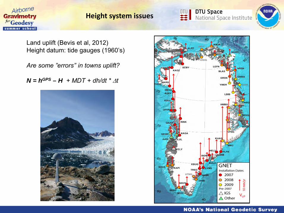
Land uplift (Bevis et al, 2012) Height datum: tide gauges (1960’s) Are some ”errors” in towns uplift? N = hGPS – H + MDT + dh/dt * ∆t
Height system issues
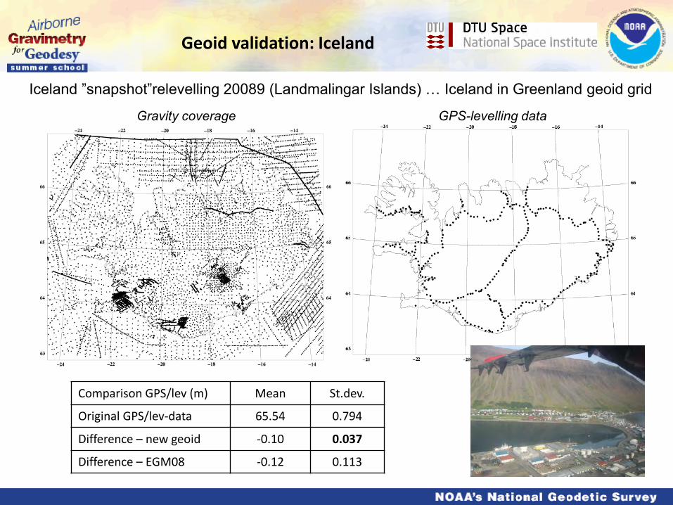
Geoid validation: Iceland
Gravity coverage GPS-levelling data
Comparison GPS/lev (m) Mean St.dev.
Original GPS/lev-data 65.54 0.794
Difference – new geoid -0.10 0.037
Difference – EGM08 -0.12 0.113
Iceland ”snapshot”relevelling 20089 (Landmalingar Islands) … Iceland in Greenland geoid grid

Greenland fjord tide gauge profiles
Sea level in fjords ”proxy” for geoid + MDT (small) – relative tidal measurements on land, GPS on ice
I
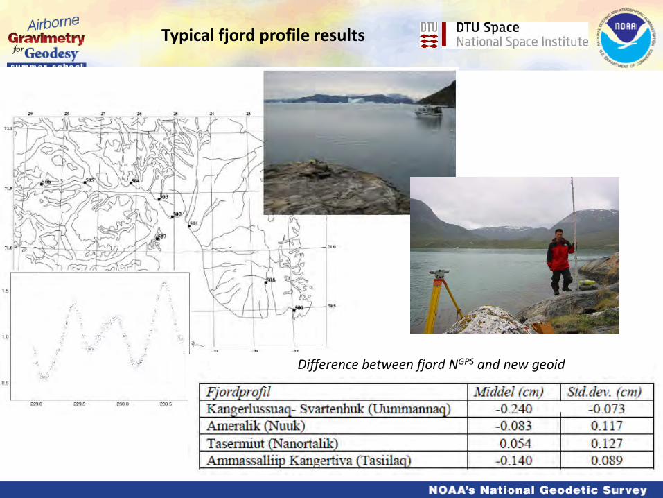
Typical fjord profile results
Difference between fjord NGPS and new geoid

Mt Everest Lhotse Makalu
A ”worst-case” geoid example - Nepal
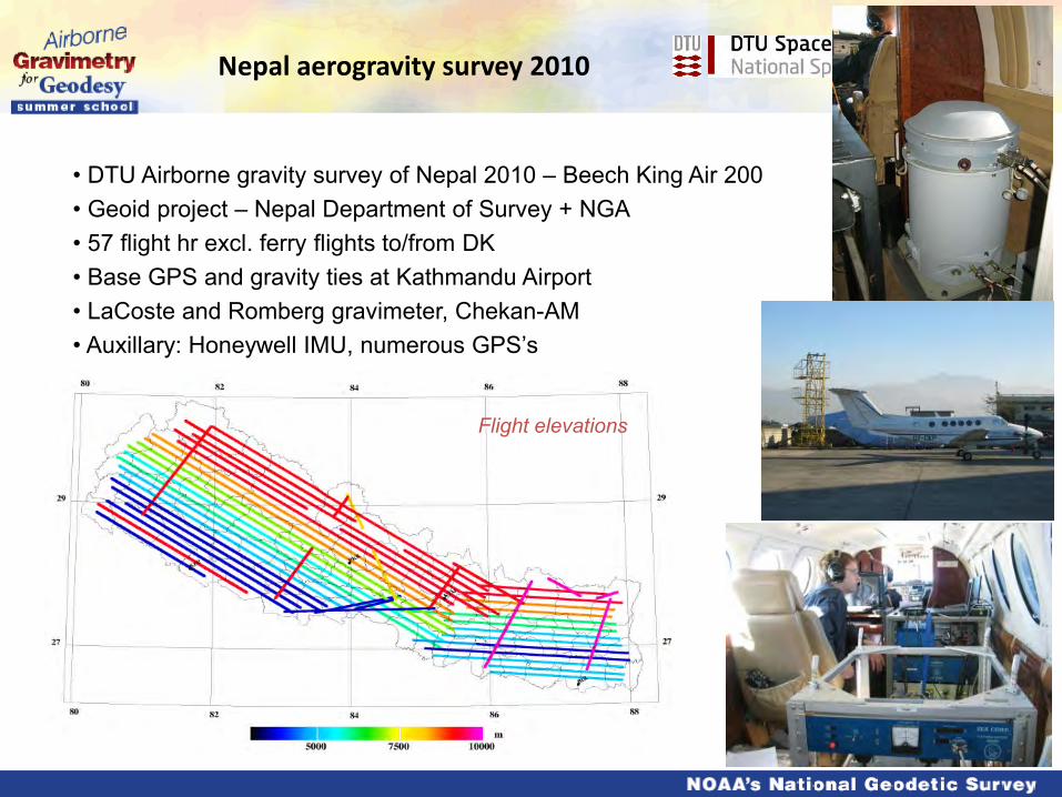
Nepal aerogravity survey 2010
• DTU Airborne gravity survey of Nepal 2010 – Beech King Air 200 • Geoid project – Nepal Department of Survey + NGA • 57 flight hr excl. ferry flights to/from DK • Base GPS and gravity ties at Kathmandu Airport • LaCoste and Romberg gravimeter, Chekan-AM • Auxillary: Honeywell IMU, numerous GPS’s
Flight elevations

Nepal SRTM terrain model
meter
Kathmandu
Everest
Annapurna

• Airborne processing with DTU-Space system – LCR and Chekan AM … cross-overs not reliable due to differing heights
Flight elevations
Free-air anomalies at altitude (mgal)
• Challenges: - mountain waves - jet streams - turbulence … especially Annapurna region
AG Results

• Chekan-AM (Russia) and LCR S-34 gravimeter processed independently Agreement between gravimeters: 4.3 mGal rms Merged set made by averaging Chekan-AM and LCR at common points • X-over errors: ~ 10 mgal rms .. cross-overs not useful for QC due to differing flight heights. After continuation to 6600 m: LCR: 4.6 mgal rms Chekan: 5.1 - Merged: 3.9 mgal rms
Free-air anomalies at altitude (mgal)
Lacoste&Romberg
Chekan-AM
AG Results
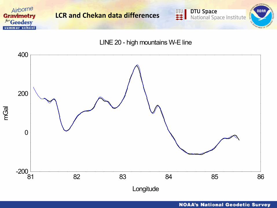
LCR and Chekan data differences
-200
0
200
400
81 82 83 84 85 86
Longitude
mG
al
LINE 20 - high mountains W-E line

LCR and Chekan – example #2
-100
0
100
200
300
81 82 83 84 85 86
LCRChekan
Longitude
mG
al
Line 24

LCR airborne data and GOCE GOCE satellite gravity @ 100 km resolution confirmed

Reference field: EGM2008 – augmented with GOCE (linear merging at degrees 80-90 and 180-190 with GOCE in middle band)
• Some special effects on airborne gravity: Terrain effects must be filtered with along-track filter corresponding to airborne gravity filter (forward/backward Butterworth filter ~ 90 sec time constant)
Data Mean Std.dev.
Airborne data -14.2 119.4
Airborne – GOCE (360) 1.4 36.5
Reduced airborne data 2.9 21.2
Surface data -87.3 103.0
Surface – GOCE -24.1 71.2
Reduced surface data -1.2 26.0
Statistics of data reductions (unit: mgal)
-200
0
200
400
600
800
0 40 80 120 160
Model covarianceEmpirical covariance
Distance (km)
mga
l**2
Covariance of airborne data
• Downward continuation of both surface and airborne data by least-squares collocation
Geoid determination – reduce steps

Reduced airborne and surface gravity
Reduced gravity data showing contribution from airborne data and surface data (changes in spacing on airborne lines due to headwind and tailwind from jet stream)

Downward continuation of all data
Deg 720 reference field

Quasigeoid contribution from spherical FFT relative to ref field
Geoid (reduced quasigeoid)

Geoid (terrain restore part)
Quasigeoid contribution from SRTM terrain 30” resolution

Difference N - ζ
Huge separation geoid-quasigeoid due to Tibetan Plateau
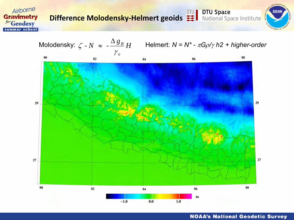
Difference Molodensky-Helmert geoids
H g - N - o
B
γζ
∆≈Molodensky: Helmert: N = N* - πGρ/γ h2 + higher-order
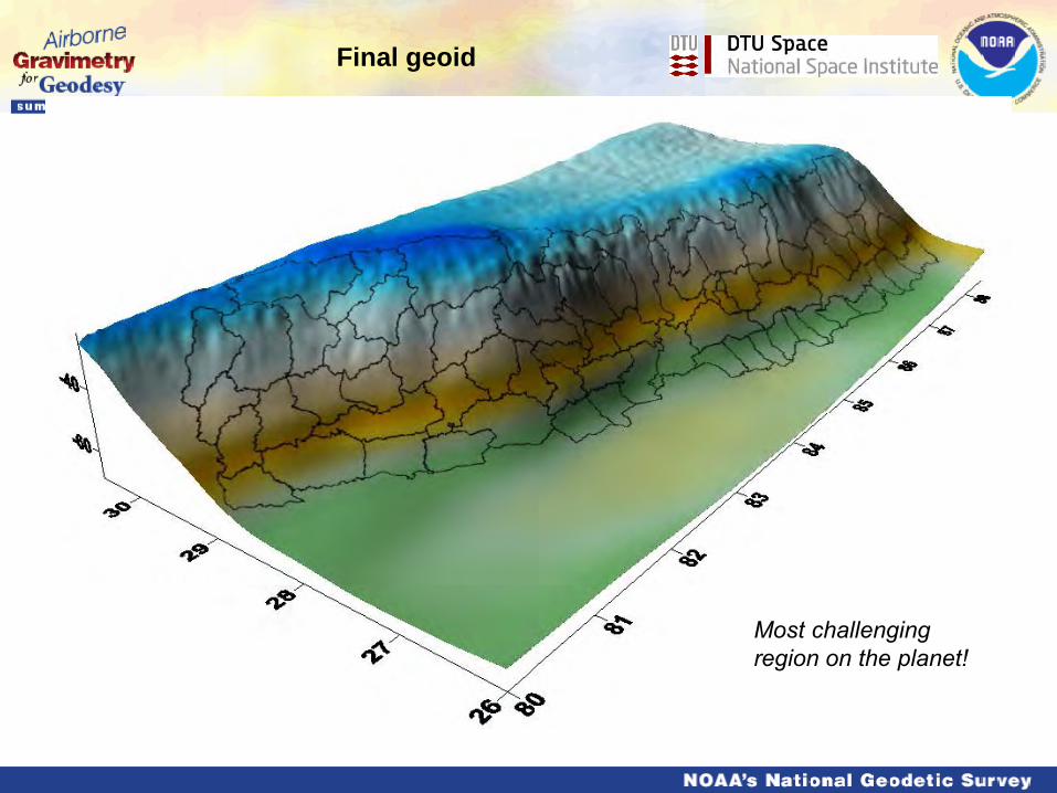
Final geoid
Most challenging region on the planet!

Geoid determination – GPS levelling comparison Very limited data set – 8 points in Kathmandu Valley (large bias due to datum error .. GPS height bias 18.5 m!)
Comparison of geoid in Kathmandu Valley
Geoid model Mean R.m.s. (m)
Geoid model (Molodensky) 19.32 0.07
Geoid model (Helmert) 19.19 0.08
GOCE 19.75 0.51
EGM08 18.51 0.30
Bias of GPS => Heights in Nepal datum lower than in (EGM08) World Height System δW0 ~ 70 cm

Height of Mt Everest
Mt Everest summit from south, Dec 17, 2010
• Classical determination: Triangulation from Himalaya foothills, Survey of India mid-1800’s (Bengal Bay datum) Chinese determination by levelling and triangulation from Yellow Sea (1970’s onwards) • GPS measurements: China and Italy – 1995, 1999, 2005 ..
Survey of Nepal Official value
8848
China (Y. Chen, 2005) 8847.93
Nat. Geographic Society (Washburn et al, 1999 - EGM96 based)
8850
Ellipsoidal height ITRF (Chen, 2005; Poretti et al, 2004)
8821.40 ±.03
Geoid height (Mol.meth) -25.71
Geoid-quasigeoid sep. -2.47
Height from Molodensky 8847.11
Geoid height (Helmert) -26.66
Height from Helmert 8848.06
Heights of Mt Everest (meter)
GRAVSOFT demo

Set of DTU-Space / UCPH (late C C Tscherning) Fortran programs … sharing common format Gridding, selection, interpolation, FFT, collocation, satellite altimetry, terrain models GEOCOL - least-squares collocation and computation of reference fields. GPCOL – least-squares collocation, especially good for downward continuation EMPCOV, COVFIT, GPFIT - empirical covariance function estimation and fitting. STOKES - Stokes' formula integration by grids. GEOFOUR, SPFOUR, SP1D - FFT gravity field modelling (planar or spherical). GEOGRID - rapid gridding by collocation or weighted means. TC - terrain effects by prism integration. TCFOUR - terrain effects by FFT methods. COVFFT - covariance functions by FFT. GEOIP - interpolation from grids to points or another grid. SELECT - thin data or make average grids. FCOMP - add/subtract data files GCOMB - add/subtract and merge grid data TCGRID - average grids and make reference topography POINTMASS - make grid or data list of point-mass effects. GEOID, GBIN - interpolation and conversion of fast binary grid format GRAVSOFT is not freeware … made available for non-commercial scientific work
GRAVSOFT
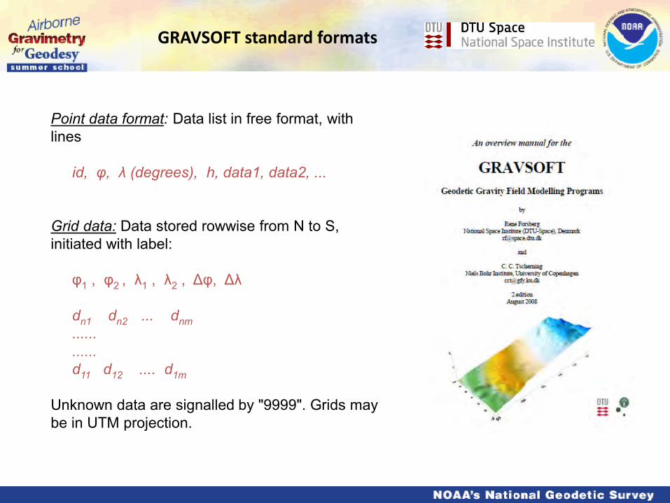
Point data format: Data list in free format, with lines id, φ, λ (degrees), h, data1, data2, ... Grid data: Data stored rowwise from N to S, initiated with label: φ1 , φ2 , λ1 , λ2 , Δφ, Δλ dn1 dn2 ... dnm ...... ...... d11 d12 .... d1m Unknown data are signalled by "9999". Grids may be in UTM projection.
GRAVSOFT standard formats

GRAVSOFT gridding
• GEOGRID central program to perform interpolation using collocation (mode 1) or weighted means (mode 2)
• Collocation: second order Gauss-Markov covariance function:
• s is the distance, C0 is the signal variance, α is the correlation length …
• Weighted means prediction (power 2) – “quick and dirty”: • In practice: select closest neighbours (e.g. 5/quadrant)
)/(0 )1()( α
αsesCsC −+=xCCs xxsx
1ˆ −=
∑
∑=
i i
i i
x
r
rs
i
2
2
1ˆ
• New 2008 module: ”fit_geoid” … does all steps of geoid fitting in one go

EF-commander – makes file navigation easy .. VI or EDITPLUS – essential with a good text editor .. MINGW32 – GNU fortran compiler SURFER – powerful graphics software (Golden Software) …. Gravsoft grid format -> surfer grid: G2SUR …. Coastline files: .BNA …. Allows posting (point plots), colour and contour plots, 3-D views .. Supplementary tool: ”job.bat” - allows UNIX-like job operations in windows (big help)! tcgrid <<! nmdtm5 nmdtmref 0 0 0 0 0 ! dummy values, may be used to select smaller area 2 2 9 9 ! average 2 x 2 cells, then do 9 x 9 moving window ! To run properly set up ”path” parameter in windows – also needed for Python to run (start – settings – control panel – system – advanced – environment variables)
Useful software for PC applications

Python interface to TC Data points to be computed
DEM file, must be larger than the data area. 2nd DEM optional
RTM reference DEM, filter with TCGRID or GFILT
Define r1 and r2
1=δg, 3=geoid, 5 = ∆g, 7 = Tzz ..
Important: prisms only used in this ”fixed” area
Reference to TC: Ohio State University report 355, 1984


