ERDC/GRL TR-20-5 Geointelligence – Geospatial Data Analysis and Decision Support Local Spatial Dispersion for Multiscale Modeling of Geospatial Data Exploring Dispersion Measures to Determine Optimal Raster Data Sample Sizes Geospatial Research Laboratory S. Bruce Blundell and Nicole M. Wayant February 2020 Approved for public release; distribution is unlimited.
Transcript
ER
DC
/G
RL T
R-2
0-5
Geointelligence – Geospatial Data Analysis and Decision Support
Local Spatial Dispersion for Multiscale
Modeling of Geospatial Data
Exploring Dispersion Measures to Determine Optimal Raster Data Sample Sizes
Ge
os
pa
tia
l R
es
ea
rch
La
bo
rato
ry
S. Bruce Blundell and Nicole M. Wayant February 2020
Approved for public release; distribution is unlimited.
The U.S. Army Engineer Research and Development Center (ERDC) solves
the nation’s toughest engineering and environmental challenges. ERDC develops
innovative solutions in civil and military engineering, geospatial sciences, water
resources, and environmental sciences for the Army, the Department of Defense,
civilian agencies, and our nation’s public good. Find out more at www.erdc.usace.army.mil.
To search for other technical reports published by ERDC, visit the ERDC online library
Exploring Dispersion Measures to Determine Optimal Raster Data Sample Sizes
S. Bruce Blundell and Nicole M. Wayant
Geospatial Research Laboratory
U.S. Army Engineer Research and Development Center
7701 Telegraph Road
Alexandria, VA 22315-3864
Final Report
Approved for public release; distribution is unlimited.
Prepared for Headquarters, U.S. Army Corps of Engineers
Washington, DC 20314-1000
Under PE 62784/Project 855/Task 22 “New and Enhanced Tools for Civil-Military
Operations”
ERDC/GRL TR-20-5 ii
Abstract
Scale, or spatial resolution, plays a key role in interpreting the spatial
structure of remote sensing imagery or other geospatially dependent data.
These data are provided at various spatial scales. Determination of an
optimal sample or pixel size can benefit geospatial models and
environmental algorithms for information extraction that require multiple
datasets at different resolutions. To address this, an analysis was
conducted of multiple scale factors of spatial resolution to determine an
optimal sample size for a geospatial dataset. Under the NET-CMO project
at ERDC-GRL, a new approach was developed and implemented for
determining optimal pixel sizes for images with disparate and
heterogeneous spatial structure. The application of local spatial dispersion
was investigated as a three-dimensional function to be optimized in a
resampled image space. Images were resampled to progressively coarser
spatial resolutions and stacked to create an image space within which
pixel-level maxima of dispersion was mapped. A weighted mean of
dispersion and sample sizes associated with the set of local maxima was
calculated to determine a single optimal sample size for an image or
dataset. This size best represents the spatial structure present in the data
and is optimal for further geospatial modeling.
DISCLAIMER: The contents of this report are not to be used for advertising, publication, or promotional purposes.
Citation of trade names does not constitute an official endorsement or approval of the use of such commercial products.
All product names and trademarks cited are the property of their respective owners. The findings of this report are not to
be construed as an official Department of the Army position unless so designated by other authorized documents.
DESTRUCTION NOTICE – Destroy by any method that will prevent disclosure of contents or
reconstruction of the document.
ERDC/GRL TR-20-5 iii
Contents
Abstract .......................................................................................................................................................... ii
Figures and Tables ........................................................................................................................................ iv
Preface ............................................................................................................................................................. v
2.3.2 Peakedness and optimal sample size .............................................................................. 11 2.4 Graphical user interface development ........................................................................ 13
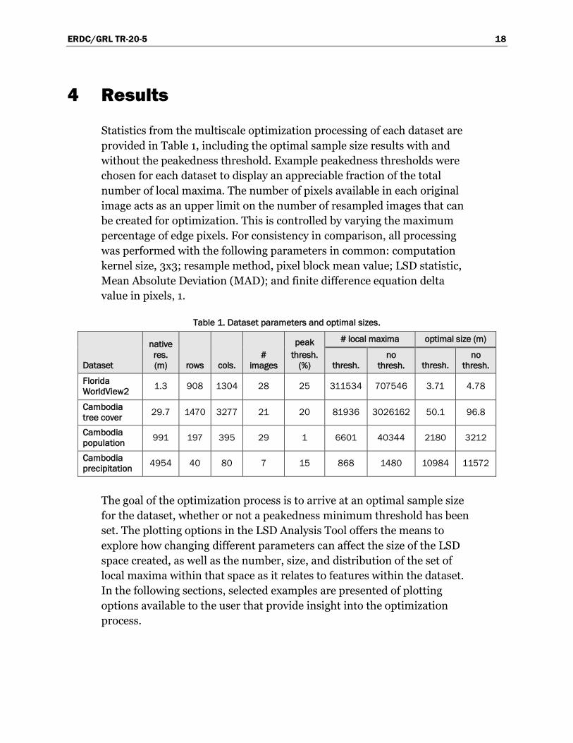
3 Data ....................................................................................................................................................... 16
Figure 23. Local maxima distribution in LSD space (Cambodia precipitation dataset).
ERDC/GRL TR-20-5 30
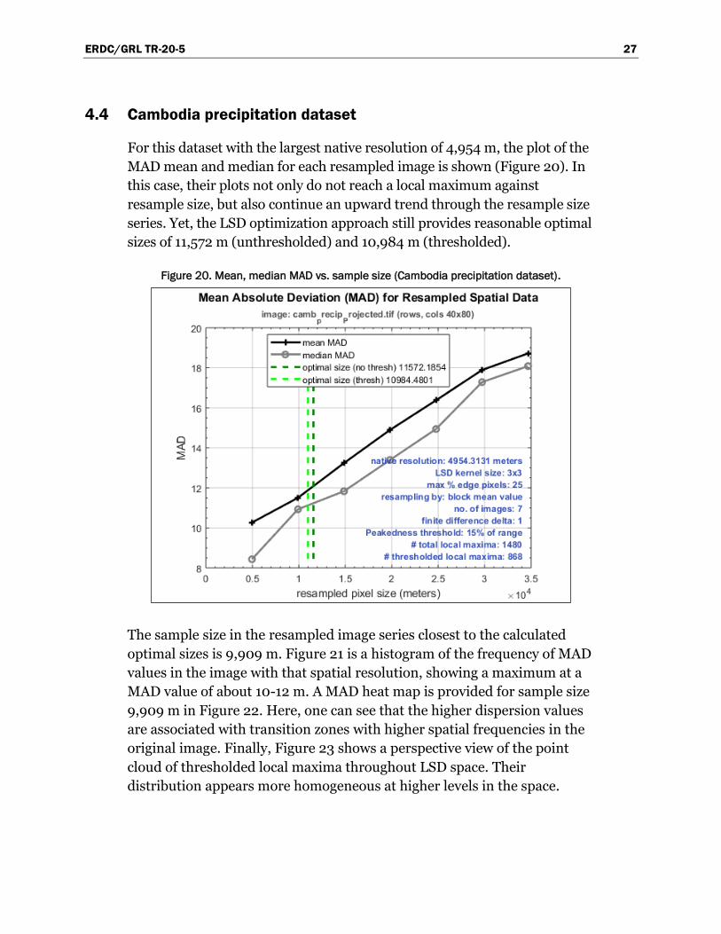
5 Discussion
In order to test this particular optimization approach, the algorithms that
implement it, and the LSD Analysis Tool, a small suite of images were
selected that represented a wide range of native resolutions, feature data
types, and spatial frequency regimes. Optimal sample sizes were
successfully calculated in all cases that scaled well with initial resolutions as
shown in Table 1. To maintain a degree of consistency, the following
processing parameters were kept constant for all four datasets: computation
kernel size, resample method, LSD statistic, and the delta interval for the
finite difference equations. At the time of writing, it is not known how
modification of these processing parameters would affect results in terms of
computed optimal sample sizes or local maxima distributions.
The results showed that optimal sizes for thresholded peakedness were
always slightly less than those that were unthresholded. The separation
depends on the choice of threshold. This suggests that local maxima with
lower values of peakedness are more concentrated near the top of LSD
space, increasing the representation of smaller resample sizes in the
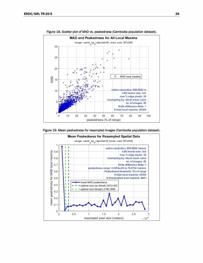
weighting process. In fact, it was found that the mean peakedness for each
image in LSD space was highest for the original resolution of each dataset
in the study. This result, as depicted in Figure 19, is typical.
In this methodology, optimal sample size results are driven by the number
and distribution of LSD local maxima as well as the LSD values associated
with each local maximum. If a peakedness threshold is chosen, the set of
local maxima is first winnowed by a minimum peakedness value. Whatever
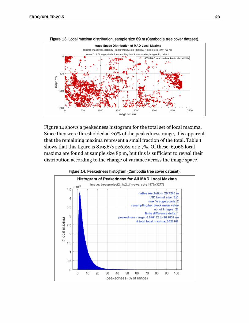
final set of maxima is used for optimization, they end up arranged in LSD
space according to feature locations at each sample size and define the
patterns of changing spatial frequencies therein (Figures 9, 13, and 17).
The setting of a peakedness threshold can be a useful tool for exploring the
distribution and peakedness of the local maxima set in LSD space by
examination of various plotting options in the LSD Analysis Tool. A
threshold is required if the retention of only high-value LSD optima for
optimal sample size calculations is indicated. However, a general strategy
has not been identified for choosing a threshold and, absent a supporting
rationale for its use, we recommend selecting the unthresholded optimal
size as a default procedure.
ERDC/GRL TR-20-5 31
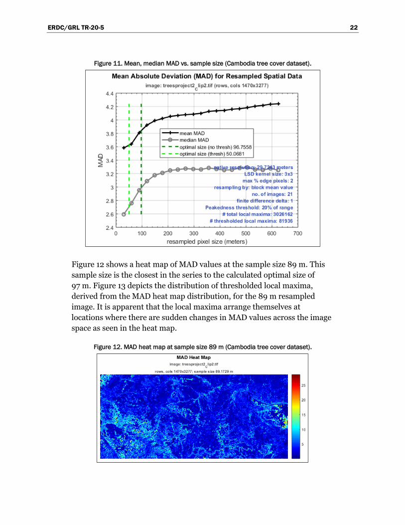
Dispersion heat maps may be useful in depicting the pattern of subtle
changes of spatial frequency inherent in the data (Figures 12, 16, and 22).
These maps may show structure not easily gleaned from a casual
examination of the original spatial data. Figure 16 shows small
concentrations of population density within the general region of higher
dispersion values around the large lake as seen in Figure 5. This pattern is
reflected in the local maxima distribution map of Figure 17. The
distribution clearly associates with population density around the lake and
along several watercourses that empty into it.
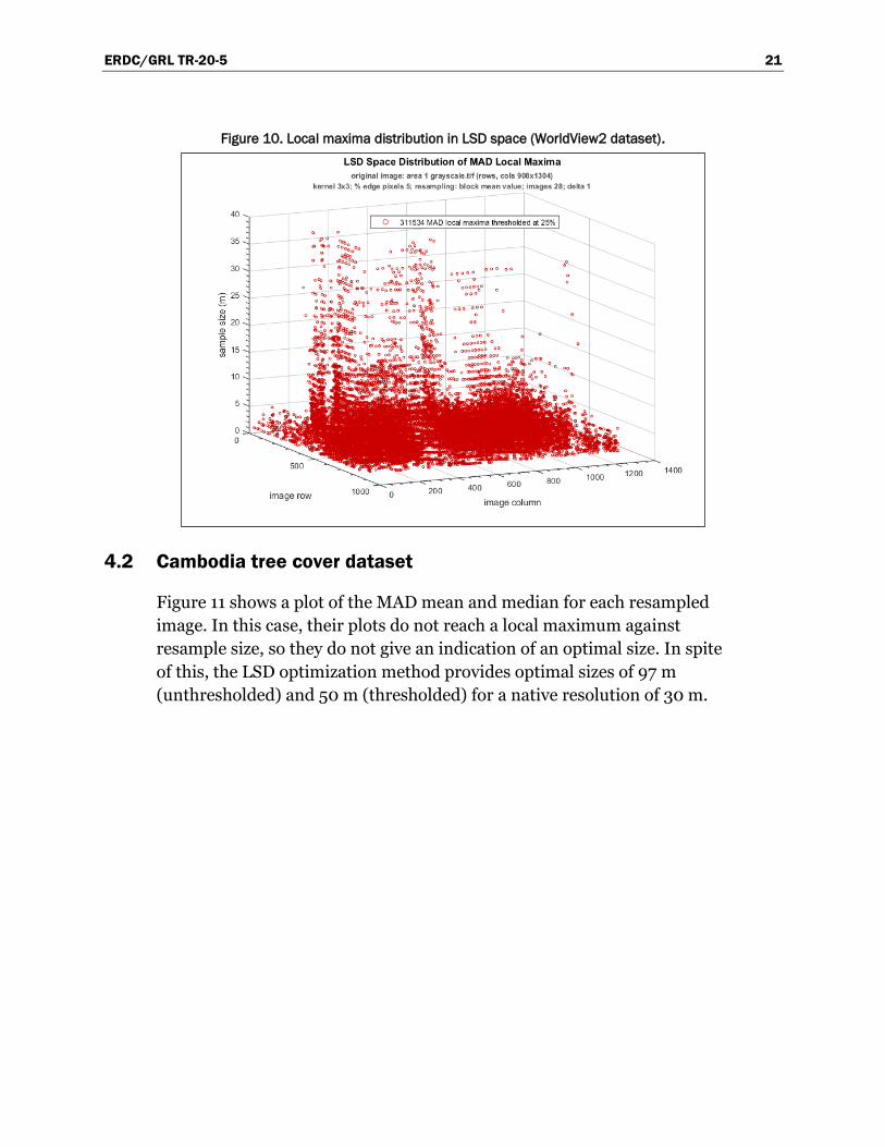
Perspective view plots of the point cloud of local maxima in LSD space can
demonstrate how they are associated with features at various sample sizes
(Figures 10 and 23). This association may extend well into the upper
reaches of LSD space as vertical features (Figure 10), or appear to acquire
a more homogeneous distribution at some point above the lowest sample
sizes (Figure 23).
The WorldView2 dataset was the only one showing a distinct maximum (at
a sample size of 6-7 m) of the mean and median for the LSD function of
sample size (Figure 7). Tree cover dominates this image. As suggested by
previous research, this LSD maximum may reflect the average size of
individual canopies visible in the image, and may be most sensitive to the
image’s predominant spatial variation. Earlier researchers have considered
the LSD maximum, where it exists, in different ways in light of their image
analysis objectives. These results indicate an optimal sample size of 4.8 m,
slightly less than that indicated by the LSD function maximum.
Results from the WorldView2 dataset suggest that this optimization
approach is in general agreement with previous work on the interpretation
of the LSD function maximum for a particular sample size. As shown in
Figures 7 and 8, it is found that a somewhat smaller sample size than that
indicated by the LSD function maximum is optimal, and may be driven by
the preponderance of local LSD maxima at lower sample sizes.
Results show that this optimization technique for a multidimensional LSD
function successfully processes the inherent dispersion of image data with
heterogeneous spatial structure. Most importantly, it provides an optimal
sample size whether or not a maximum for the mean LSD function of
sample size exists (Figures 11, 15, and 20).
ERDC/GRL TR-20-5 32
6 Summary and Conclusions
The spatial characteristics of continuously varying phenomena on the
Earth’s surface directly inform remotely sensed data or other types of
environmental information collected in a geospatial context. The spatial
domain or structure of this data can be used to optimize its interpretation
or extraction of spatial information. Effective mapping or modeling of
spatially dependent information requires capturing the spatial variation
patterns of features of interest. A key consideration in image analysis is the
relationship between spatial resolution and the spatial frequency structure
of features found in the image data.
In this work, this relationship was examined through a multiscale
modeling approach to determine an optimal sample size for raster images
containing remotely sensed or other environmental data with variable
spatial structure. Resampling an image dataset in this way can increase the
efficiency of image processing functions, such as feature segmentation or
of geospatial models, such as that employed in the NET-CMO project at
ERDC-GRL. Four image datasets were analyzed with disparate native
resolutions collected over Florida and Cambodia. These datasets depict a
variety of environmental feature data with heterogeneous spatial
structure. In each case, a multidimensional dispersion space was created
from which sets of local maxima were extracted. These local maxima were
used in a weighted mean formulation to compute optimal sample sizes
that did not depend on the single-variable functional relationship between
mean dispersion and resample size. This approach captures the locality of
variance in heterogeneous spatial datasets rather than relying on an
overall mean dispersion value for each resampled image.
A useful tool and user interface was created, the LSD Analysis Tool, to
exercise our algorithmic approach and allow a user to process a dataset
while in control of particular processing parameters. Various plotting
options display relationships among LSD values, local LSD maxima,
maxima peakedness, and LSD space locations. These output features and
level of user control provide for repeated experimentation and a better
understanding of the spatial structure of the data.
The authors believe that this multiscale modeling approach to optimizing
sample size is an effective and robust method as applied to geospatial data.
ERDC/GRL TR-20-5 33
References
Atkinson, P. M., and P. J. Curran. 1995. Defining an optimal size of support for remote sensing investigations. IEEE Transactions on Geoscience and Remote Sensing 33:768-776.
Chapra, S. C., and R. P. Canale. 2002. Numerical methods for engineers: with software and programming applications. Fourth ed., p. 355. New York: McGraw-Hill.
Costanza, R., and T. Maxwell. 1994. Resolution and predictability: An approach to the scaling problem. Landscape Ecology 9(1):47-57.
Curran, P. J. 2001. Remote sensing: Using the spatial domain. Environmental and Ecological Statistics 8:331-344.
Curran, P. J., P. M. Atkinson, G. M. Foody, and E. J. Milton. 2000. Linking remote sensing, land cover, and disease. Advances in Parasitology 47:37-81.
Goodchild, M. F. 2011. Scale in GIS: An overview. Geomorphology 130:5-9.
Marceau, D. J., D. J. Gratton, R. A. Fournier, and J. P. Fortin. 1994. Remote sensing and the measurement of geographical entities in a forested environment 2. The optimal spatial resolution. Remote Sensing of Environment 49:105-117.
McCloy, K. R., and P .K. Bøcher. 2007. Optimizing image resolution to maximize the accuracy of hard classification. Photogrammetric Engineering and Remote Sensing 73(8):893-903.
Rahman, A. F., J. A. Gamon, D. A. Sims, and M. Schmidts. 2003. Optimum pixel size for hyperspectral studies of ecosystem function in southern California chaparral and grassland. Remote Sensing of Environment 84:192-207.
Richards, J. A., and X. Jia. 1999. Remote sensing digital image analysis: an introduction. 3rd ed., pp. 162-164. Berlin Heidelberg: Springer-Verlag.
Woodcock, C. E., and A. H. Strahler. 1987. The factor of scale in remote sensing. Remote Sensing of Environment 21:311-322.
ERDC/GRL TR-20-5 34
Acronyms and Abbreviations
Acronym Meaning
ERDC Engineer Research and Development Center
GRL Geospatial Research Laboratory
GSD Ground Sample Distance
GUI Graphical User Interface
LSD Local Spatial Dispersion
LSV Local Spatial Variance
MAD Mean Absolute Deviation
NET-CMO New and Enhanced Tools for Civil-Military Operations
USACE U.S. Army Corps of Engineers
REPORT DOCUMENTATION PAGE Form Approved OMB No. 0704-0188
Public reporting burden for this collection of information is estimated to average 1 hour per response, including the time for reviewing instructions, searching existing data sources, gathering and maintaining the data needed, and completing and reviewing this collection of information. Send comments regarding this burden estimate or any other aspect of this collection of information, including suggestions for reducing this burden to Department of Defense, Washington Headquarters Services, Directorate for Information Operations and Reports (0704-0188), 1215 Jefferson Davis Highway, Suite 1204, Arlington, VA 22202-4302. Respondents should be aware that notwithstanding any other provision of law, no person shall be subject to any penalty for failing to comply with a collection of information if it does not display a currently valid OMB control number. PLEASE DO NOT RETURN YOUR FORM TO THE ABOVE ADDRESS.
1. REPORT DATE (DD-MM-YYYY)
February 2020
2. REPORT TYPE
Final report 3. DATES COVERED (From - To)
4. TITLE AND SUBTITLE
Local Spatial Dispersion for Multiscale Modeling of Geospatial Data: Exploring Dispersion
Measures to Determine Optimal Raster Data Sample Sizes
5a. CONTRACT NUMBER
5b. GRANT NUMBER
5c. PROGRAM ELEMENT NUMBER
62784
6. AUTHOR(S)
S. Bruce Blundell and Nicole M. Wayant
5d. PROJECT NUMBER
855
5e. TASK NUMBER
22
5f. WORK UNIT NUMBER
7. PERFORMING ORGANIZATION NAME(S) AND ADDRESS(ES) 8. PERFORMING ORGANIZATION REPORT NUMBER
Geospatial Research Laboratory
U.S. Army Engineer Research and Development Center