Discrete Comput Geom 4:591-604 (1989) Geom etryDi .rete & C4nntmtatk~tal

A Linear-Time Algorithm for Computing the Voronoi Diagram of a Convex Polygon*

Alok Aggarwal, 1 Leonidas J. Guibas , 2"3 James Saxe, 3 and Peter W. Shor 4

IBM T. J. Watson Research Center, P.O. Box 218, Yorktown Heights, NY 10598, USA

2 Department of Computer Science, Stanford University, Stanford, CA 94305, USA

3 DEC Systems Research Center, 130 Lytton Avenue, Palo Alto, CA 94301, USA

4 AT&T Bell Laboratories, 600 Mountain Avenue, Murray Hill, NJ 07974, USA

Abstract. We present an algorithm for computing certain kinds of three- dimensional convex hulls in linear time. Using this algorithm, we show that the Voronoi diagram of n sites in the plane can be computed in O(n) time when these sites form the vertices of a convex polygon in, say, counterclockwise order. This settles an open problem in computational geometry. Our techniques can also be used to obtain linear-time algorithms for computing the furthest-site Voronoi diagram and the medial axis of a convex polygon and for deleting a site from a general planar Voronoi diagram.

1. Introduction

Suppose we are given a set S of n sites, S={p~,p: , . . . ,p ,} , in the Eucl idean plane. For any two sites Pi and p~, the set of points closer to p~ than to pj is the open hal f -p lane con ta in ing Pi that is del imited by the perpendicular bisector of Pi-'~j. Let us denote this hal f -plane by H(p~, pj). The locus of points closer to p~ than to any other site, which we denote by V(i), is the intersect ion of n - 1 half-planes, i.e., V(i)=f'~i,,j H(p~, pj); V(i) is called the Voronoi region associ-

ated with p~. The n regions V(i), which may be u n b o u n d e d , divide the p lane

* This research began while the first and fourth authors were visiting the Mathematical Sciences Research Institute in Berkeley, California. Work by the fourth author was supported in part by NSF Grant No. 8120790.

592 A. Aggarwal, L. J. Guibas, J. Saxe, and P. W. Shot

into a convex net usually called the Voronoi diagram of S. The straight-line dual of the Voronoi diagram is called the Delaunay triangulation of $. Because of the extensive applications of Voronoi diagrams and Delaunay triangulations in diverse areas of science and technology, the problem of computing these structures has received considerable attention in recent years. In 1978 Shamos [10] showed that the Voronoi diagram of n sites in the plane can be computed in O(n log n) time, and, furthermore, that this bound is optimal (up to a multiplicative constant) since the convex hull of these sites can be extracted in O(n) time from the Voronoi diagram.

The f~(n log n) lower bound in Shamos [10] does not apply when the input sites are the vertices of a convex polygon (given in counterclockwise order) rather than an arbitrary set of points in the plane. Consequently, it has remained an open problem whether the Voronoi diagram of the vertices of a convex polygon can be computed in linear time [9]. In this paper we settle this question in the affirmative by demonstrating a linear-time algorithm for this problem. We also show that the technique used here can be used to reduce the time complexity of several other problems. This technique has a number of novel aspects that make it interesting in its own right.

Consider the following problem: construct the convex hull of a set of n given points in three dimensions when it is known that the projections of the given points on the xy plane form the vertices of a convex polygon and the counterclock- wise order of these projections in this plane is provided (see Fig. 1). The main result of this paper is that this problem can be solved in linear time. By using the lifting map given by Guibas and Stolfi [2] that takes (x, y) to (x, y, x2+y2), we can reduce the problem of constructing the closest-site Voronoi diagram for a set of n vertices of a convex polygon given in order to a special case of this problem and hence we can obtain the Voronoi diagram of such a set in linear time.

The geometric dual of this problem is also interesting. By dualizing our algorithm, we obtain the following: suppose we are given n half-spaces H~, H2,.. . , H,, in three dimensions. Suppose furthermore that we are also given a plane p on which these half-spaces define n half-planes intersecting in a convex

il I I I I I I I

Fig. 1. We can

/d

! i i i ~ \ V I

I I i ' ' ' ' " i

! I i i ! il !

find the convex hull of points a-j in linear time.

Voronoi Diagrams of Convex Polygons 593

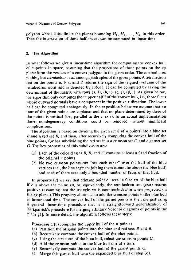
polygon whose sides lie on the planes bounding H~, H 2 , . . . , Hn, in this order. Then the intersection of these half-spaces can be computed in linear time.

2. The Algorithm

In what follows we give a linear-time algorithm for computing the convex hull of n points in space, assuming that the projections of these points on the xy plane form the vertices of a convex polygon in the given order. The method uses nothing but tetrahedron tests among quadruples of the given points. A tetrahedron test on the points a, b, c, and d returns the sign of the (signed) volume of the tetrahedron abcd and is denoted by (abcd). It can be computed by taking the determinant of the matrix with rows (a, 1), (b, 1), (c, 1), (d, 1). As given below, the algorithm only computes the "upper half" of the convex hull, i.e., those faces whose outward normals have a component in the positive z direction. The lower half can be computed analogously. In the exposition below we assume that no four of the given points are coplanar and that no plane determined by three of the points is vertical (i.e., parallel to the z axis). In an actual implementation these nondegeneracy conditions could be removed without significant complications.

The algorithm is based on dividing the given set S of n points into a blue set B and a red set R, and then, after recursively computing the convex hull of the blue points, further subdividing the red set into a crimson set C and a garnet set G. The key properties of this subdivision are:

(1) Each of the color classes B, R, and C contains at least a fixed fraction of the original n points.

(2) No two crimson points can "see each other" over the hull of the blue vertices (i.e., the line segment joining them cannot lie above the blue hull) and each of them sees only a bounded number of faces of that hull.

In property (2) we say that crimson point c "sees" a face rst of the blue hull if c is above the plane rst, or, equivalently, the tetrahedron test (crst) returns positive (assuming that the triangle rst is counterclockwise when projected on the xy plane.) This property allows us to add the crimson points to the blue hull in linear total time. The convex hull of the garnet points is then merged using a general linear-time procedure that is a straightforward generalization of Kirkpatrick's procedure for merging arbitrary Voronoi diagrams of points in the plane [3]. In more detail, the algorithm follows these steps:

Procedure CH (computes the upper hull of the n points) (a) Partition the original points into the blue and red sets B and R. (b) Recursively compute the convex hull of the blue points. (c) Using the structure of the blue hull, select the crimson points C. (d) Add the crimson points to the blue hull one at a time. (e) Recursively compute the convex hull of the garnet points G. (f) Merge this garnet hull with the expanded blue hull of step (d).

594 A. Aggarwal, L. J. Guibas, J. Saxe, and P. W. Shor

What makes the algorithm linear is the ability to add a fixed fraction of the red points to the blue hull at constant cost per point. The points added are the crimson points, that see disjoint subsets of the faces in the blue hull.

We now give some additional details. First we describe how the blue-red partitioning is done (in linear time).

Go counterclockwise around the convex polygon of projections on the xy plane. I f a, b, c, d are four consecutive points (more precisely, points whose projections are consecutive), then label the edge bc as D (for down) if triangle abc is above bcd (a "sees" bcd) and as U (for up) otherwise. This labeling is well defined, since the two triangles in question always overlap in z, because of convexity. The label o f an edge can be determined by using a single tetrahedron test (e.g., edge bc is labeled D iff test abcd is positive). Label each vertex by the labels of its two adjacent edges in counterclockwise order. Vertex labels can thus be UU, DD, UD, or DU (see Fig. 2).

Now color the vertices red or blue (as in Fig. 2) so that the following conditions are met:

(1) All UD vertices are colored red. (2) No two consecutive vertices are red. (3) No three consecutive vertices are blue.

It is easy to check that such a coloring is always possible: first color all the UD vertices red; clearly no two of them can be adjacent. Then consider each of the uncolored intervals thus formed. Proceeding counterclockwise from each partitioning UD vertex, color the remaining vertices alternatively blue and red. I f the interval has even length, then the last few vertices will be colored " . . . RBRR," where the last R belongs to the next UD vertex. Since two consecu- tive reds are not allowed, we change the last interval vertex to a blue, thus

Fig. 2.

13

Labeling the points blue and red. Blue vertices are dark and red are light.

Voronoi Diagrams of Convex Polygons 595

obtaining " . . . RBBR," which obeys the above conditions. Any coloring satisfying the above conditions provides a partitioning that has the following two additional properties:

(1) The number of blue and red vertices are each at least a fixed fraction of n. (2) No pair of red vertices consecutive in the circular ordering can "see each

other" across the blue hull.

The second assertion requires that we check two situations (R and B refer to vertex colors; ordering is counterclockwise). In each case we establish that the edge connecting two consecutive red vertices passes below some edge belonging to the blue hull.

(a) The RBR situation: the color sequence must be " . . . BtRBRIB . . . . " If the central blue vertex is a UU, then the RR diagonal is below the blue diagonal o l ° B o lB. I f it is a DD, then the RR diagonal is below the blue diagonal B I ° B o i °; and if it is a DU, then it is below both. In either case, RR cannot be above the blue hull (again "'below" here is to be understot~d in terms of the appropriate tetrahedron test). For example, in Fig. 2 the red diagonal ac is below the blue diagonals jb and bd.

(b) The RBBR situation: the color sequence must be " . . . BIRBBR[B....'" The two central blue vertices must arise out of an edge label sequence that is UUU, DUU, DDU, or DDD. In the * UU cases, the RR diagonal is below the blue diagonal o I o o B o IB, and in the DD* cases it is below the blue diagonal B I ° B o o [ o. For example, in Fig. 2 the red diagonal eh is below the blue diagonal gi.

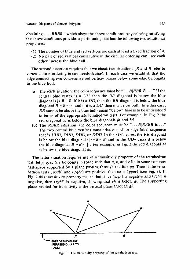
The latter situation requires use of a transitivity property of the tetrahedron test: let p, q, a, b, c be points in space such that a, b, and c lie in some comrr~on half-space supported by a plane passing through the line pq. Then if the tetra- hedron tests (pqab) and (pqbc) are positive, then so is (pqac) (see Fig. 3). In Fig. 2 this transitivity property means that since (efgh) is negative and (fghi) is negative, then (eghi) is negative, showing that eh is below gi. The supporting plane needed for transitivity is the vertical plane through gh.

b

p q

SUPPORTING PLANE (PERPENDICULAR TO PAGE)

Fig. 3. The transitivity property of the tetrahedron test,

596 A. Aggarwal, L. J. Guibas, J. Saxe, and P. W. Shor

10 11 I 9

1

2

5

Fig. 4. The topological ordering of vertices around a tree.

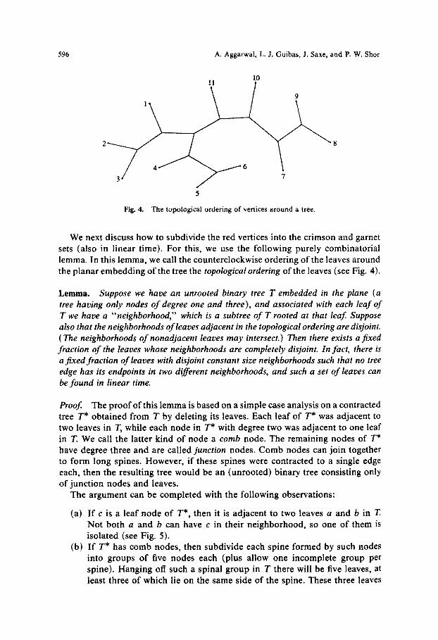
We next discuss how to subdivide the red vertices into the crimson and garnet sets (also in linear time). For this, we use the following purely combinatorial lemma. In this lemma, we call the counterclockwise ordering of the leaves around the planar embedding of the tree the topological ordering of the leaves (see Fig. 4).

Lemma. Suppose we have an unrooted binary tree T embedded in the plane ( a tree having only nodes of degree one and three), and associated with each leaf of T we have a "neighborhood," which is a subtree of T rooted at that leaf. Suppose also that the neighborhoods of leaves adjacent in the topological ordering are disjoint. (The neighborhoods of nonadjacent leaves may intersect.) Then there exists a fixed fraction of the leaves whose neighborhoods are completely disjoint. In fact, there is a fixed fraction of leaves with disjoint constant size neighborhoods such that no tree edge has its endpoints in two different neighborhoods, and such a set of leaves can be found in linear time.

Proof. The proof of this lemma is based on a simple case analysis on a contracted tree T* obtained from T by deleting its leaves. Each leaf of T* was adjacent to two leaves in T, while each node in T* with degree two was adjacent to one leaf in T. We call the latter kind of node a comb node. The remaining nodes of T* have degree three and are called junction nodes. Comb nodes can join together to form long spines. However, if these spines were contracted to a single edge each, then the resulting tree would be an (unrooted) binary tree consisting only of junction nodes and leaves.

The argument can be completed with the following observations:

(a) If c is a leaf node of T*, then it is adjacent to two leaves a and b in T. Not both a and b can have c in their neighborhood, so one of them is isolated (see Fig. 5).

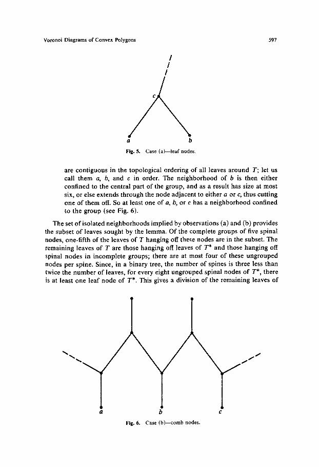
(b) If T* has comb nodes, then subdivide each spine formed by such nodes into groups of five nodes each (plus allow one incomplete group per spine). Hanging off such a spinal group in T there will be five leaves, at least three of which lie on the same side of the spine. These three leaves

Voronoi Diagrams of Convex Polygons 597

/ /

/

a b

Fig. 5. Case (a)--leaf nodes.

are contiguous in the topological ordering of all leaves around T; let us call them a, b, and c in order. The neighborhood of b is then either confined to the central part of the group, and as a result has size at most six, or else extends through the node adjacent to either a or c, thus cutting one of them off. So at least one of a, b, or c has a neighborhood confined to the group (see Fig. 6).

The set of isolated neighborhoods implied by observations (a) and (b) provides the subset of leaves sought by the lemma. Of the complete groups of five spinal nodes, one-fifth of the leaves of T hanging off these nodes are in the subset. The remaining leaves of T are those hanging off leaves of T* and those hanging off

spinal nodes in incomplete groups; there are at most four of these ungrouped nodes per spine. Since, in a binary tree, the number of spines is three less than twice the number of leaves, for every eight ungrouped spinal nodes of T*, there is at least one leaf node of T*. This gives a division of the remaining leaves of

a b c

Fig. 6. Case (b)--comb nodes.

598 A. Aggarwal, L. J. Guibas, J. Saxe, and P. W. Shor

T into groups of at most ten (eight or less hanging off spinal nodes of T*, and two hanging off a leaf node of T*), of which one will be in our set. Our set thus comprises at least one-tenth of all the leaves of T.

Furthermore, we can find this set in linear time. We first divide the spinal nodes of T* into groups of five. This can be done using depth-first search. We then check the neighborhoods of leaves of T. If a neighborhood has the right structure, we add it to our set. If we find a neighborhood is too large, then we can stop checking it after we know it has size more than six. (This assumes that we can incrementally compute a neighborhood of size k in O(k) time.) []

In our case the tree T is that given by the (planar graph) dual of the blue convex hull, where each face of the blue hull corresponds to an internal node of the tree T. The leaves of the tree T correspond to the outer edges of the blue hull, where an outer edge is an edge adjacent to only one face of the upper hull. The red points correspond to some of these leaves, and the neighborhood of a red leaf is the set of blue hull faces visible from the corresponding red point. If two red points are above the same blue face, then they can see each other over the blue hull. Thus, the "nonvisibility" condition between adjacent red points implies the disjoint neighborhoods condition of the lemma above. Since we have allowed up to two consecutive blue vertices in the original ordering, there may be some outer edges of the blue hull with no associated red point. However, this cannot be the case for more than half of the outer blue edges and so the corresponding "blue" leaves and all resulting degree-two nodes can be contracted out of T without affecting the tree size by more than a constant factor. We can now apply the above combinatorial lemma to this modified tree. The set of leaves with disjoint neighborhoods guaranteed by the lemma is the set of crimson points. The rest of the red points are the garnet ones. No two crimson points can see each other over the blue hull. If two points could see each other, then some blue edge would be visible from both points; this situation is impossible by the above lemma (it corresponds to a tree edge with endpoints in two different neighborhoods).

All other steps in the algorithm are done in the obvious way. Steps (c) and (d) are accomplished by exploring the collection of visible faces of the blue hull from each crimson point. For step (c), the number of faces that need to be tested for visibility per crimson point is proportional to the size of the neighborhood of the corresponding leaf in the tree. Because there is at most one blue leaf between two adjacent red leaves (in the topological order), replacing the blue nodes we contracted can increase the size of a neighborhood by at most a constant factor. Thus, even after the contracted blue nodes are replaced, neighborhoods of crimson points cannot have more than constant size. For step (d), since each crimson point sees only blue points, the crimson points can be added in incremental fashion in total linear time.

The convex hull of the garnet points is then computed recursively in step (e), and finally that hull is merged with the blue-crimson hull that is already available, again in linear total time.

Voronoi Diagrams of Convex Polygons 599

We must still show how to merge the garnet convex hull with the blue hull in linear time. (We recolor crimson points blue for this part.) This is done using a simple algorithm based on Kirkpatrick's Voronoi merging algorithm [3]. Consider the final convex hull. I f all the faces are triangles, it is easy to see that every face either has no or two "dichromatic" edges, where a dichromatic edge goes between a garnet and a blue point. To find the final hull, it suffices to find all dichromatic faces, since the remaining monochromatic faces from the red and blue convex hulls can easily be inserted. I f we consider two faces sharing a dichromatic edge to be connected, then the dichromatic faces form chains, each chain starting and ending with a face containing a dichromatic outer edge. There can be no interior cycles of dichromatic faces because the planar dual to the edge graph (of the upper hull) is a tree. To find all the dichromatic faces, we start with a dichromatic outer edge, find the face containing it, find the other dichromatic edge contained in this face, proceed to the other face on this dichromatic edge, and so on. When we reach the (dichromatic) outer edge at the end of this chain, we find another dichromatic outer edge and follow the chain of dichromatic faces leading from it. We continue until we have processed all dichromatic outer edges. Finding the dichromatic outer edges is easy, since all outer edges can be obtained directly from the input.

To go into the details of this procedure, we must first describe the data structures we need. For each vertex of the blue (garnet) hull, we use a linked list containing the blue (garnet) edges incident to that vertex in cyclic order. This list begins (and ends) with an outer edge of the blue (garnet) hull. We are thus able to use this list to explore the monochromatic edges around a vertex in clockwise or counterclockwise order. (In the following, when we talk about the cyclic order of edges around a vertex, we mean cyclic order as seen from above.)

Suppose we know a dichromatic edge ab (assume a is garnet and b blue) and we want to find a face containing it. In general, either ab is an outer edge, or we have already found one dichromatic face abc containing ab, so we need only find the dichromatic face on a given side of ab. There must be one monochromatic edge in the face we want, and it must contain either a or b. We already know all the monochromatic edges adjacent to a and b. We need only check these edges to see which one gives us the uppermost face meeting edge ab on the proper side of this edge. To do this, we first find a candidate face with a monochromatic garnet edge, next find a candidate edge with a monochromatic blue edge, and then compare these two faces to see which is above the other. (In Fig. 7 we need to check faces generated by the garnet edges ag3, ag4, and ags and the blue edges bb3 and bb4.) To find the candidate face containing a garnet edge quickly, we use the following fact: if we check, starting from either end of the cyclic list of garnet edges through a and on the proper side of ab, whether each face we test is above the following one, then the first face we find that is above the following one is the garnet candidate face (i.e., it is above every other face formed by b and a garnet edge through a that lies on the proper side of ab.) This is a consequence of the convexity of the garnet hull and the fact the b is outside this hull. I f we start, not with the outer edge of the garnet hull containing

600 A. Aggarwal, L J. Guibas, J. Saxe, and P. W. Shor

g3 ~ g~

~ . . . . . . . . . . ~ a

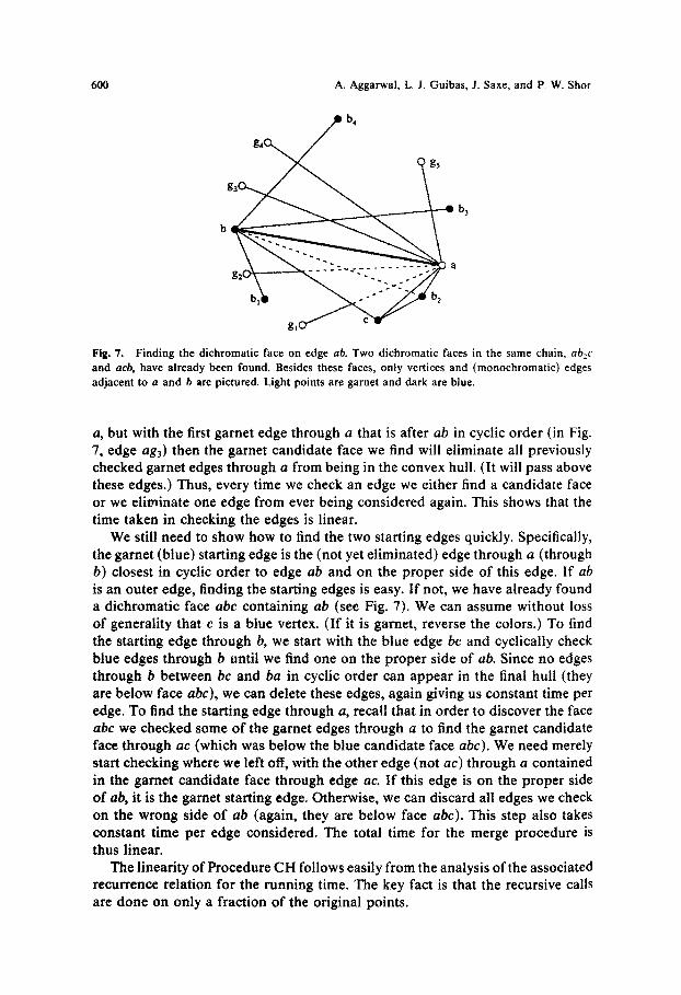
Fig. 7. Finding the dichromatic face on edge ab. Two dichromatic faces in the same chain, ab2c and acb, have already been found. Besides these faces, only vertices and (monochromatic) edges adjacent to a and b are pictured. Light points are garnet and dark are blue.

a, but with the first garnet edge through a that is after ab in cyclic order (in Fig. 7, edge ag3) then the garnet candidate face we find will eliminate all previously checked garnet edges through a from being in the convex hull. (It will pass above these edges.) Thus, every time we check an edge we either find a candidate face or we eliminate one edge from ever being considered again. This shows that the time taken in checking the edges is linear.

We still need to show how to find the two starting edges quickly. Specifically, the garnet (blue) starting edge is the (not yet eliminated) edge through a (through b) closest in cyclic order to edge ab and on the proper side of this edge. If ab is an outer edge, finding the starting edges is easy. If not, we have already found a dichromatic face abc containing ab (see Fig. 7). We can assume without loss of generality that c is a blue vertex. ( I f it is garnet, reverse the colors.) To find the starting edge through b, we start with the blue edge bc and cyclically check blue edges through b until we find one on the proper side of ab. Since no edges through b between bc and ba in cyclic order can appear in the final hull (they are below face abc), we can delete these edges, again giving us constant time per edge. To find the starting edge through a, recall that in order to discover the face abc we checked some of the garnet edges through a to find the garnet candidate face through ac (which was below the blue candidate face abc). We need merely start checking where we left off, with the other edge (not ac) through a contained in the garnet candidate face through edge ac. If this edge is on the proper side of ab, it is the garnet starting edge. Otherwise, we can discard all edges we check on the wrong side of ab (again, they are below face abc). This step also takes constant time per edge considered. The total time for the merge procedure is thus linear.

The lineadty of Procedure CH follows easily from the analysis of the associated recurrence relation for the running time. The key fact is that the recursive calls are done on only a fraction of the original points.

Voronoi Diagrams of Convex Polygons 601

3. Generalizations

Where was convexity of the xy projection used in this argument? It was implicitly used in two places: in the definition of the U and D labels for the edges, and in the transitivity of the tetrahedron test. In both places a weaker condition obviously suffices. The weaker condition states that through every side of our polygon in space, there should be a plane that leaves all other vertices in the same half-space. Furthermore, this should also be true for the vertices of any subpolygon that is defined by taking a subsequence of the vertices of the original polygon.

We can think of what we have proven as asserting that if we take a convex polygonal cylinder in space and draw a polygon with one side per face on the cylinder, then it is possible to compute the convex hull of that polygon in linear time. By the above remark, this obviously generalizes to convex cones. The cylinder is then the special case when the apex of the cone goes to infinity.

4. Consequences

The above result implies that the Voronoi diagram and Delaunay triangulation of a convex polygon in the plane can be computed in linear time. We simply use the standard lifting map onto the paraboloid of revolution z = x 2 + y2 and compute the lower hull of the lifted points [2]. This gives the Delaunay triangulation, which we can dualize to obtain the Voronoi diagram.

The furthest-site Voronoi diagram for a set of n given sites P l , . - - , Pn, is a partition of the plane into convex regions, V(pl) , . . . , V(pn), such that any point in V(pi) is farther from site p~ than from any other site. By using the same lifting map onto z = x: + y2, but computing the upper hull, we can construct the furthest- site Voronoi diagram in linear time when given the vertices of a convex polygon in counterclockwise order.

Our result also implies that we can delete a vertex from a convex polyhedron and then recompute the convex hull of the remaining vertices in linear time. This is so because the neighbor vertices of the vertex being deleted form a polygon on a convex cone, in the above sense. A corollary of the above observation is that it is possible to delete a site from a Voronoi diagram in the plane and update the diagram in linear time.

In the algorithm of Lee [5] for finding the kth order Voronoi diagram, the result of deleting a site from a Voronoi diagram is repeatedly calculated. Using our linear-time procedure instead of the standard O(n log n) time we reduce the time of Lee's algorithm from O(nk 2 log n) to O(nk2+ n log n).

Given two convex polygons, P and Q, with n and m vertices, respectively, consider the problem of finding the closest (or the furthest) vertex of P for every vertex of Q. Clearly, this problem can be solved in O((m + n)log(m + n)) time using the Voronoi diagram of P and any of the methods for point location in planar subdivisions that have been extensively studied in the literature. (See [4] and [9], for example.) However, we can use the linear-time algorithm given in

602 A. Aggarwal, L. J. Guibas, J. Saxe, and P. W. Shor

this paper to solve this problem in O(m+ n) time as follows: construct the closest-site Voronoi diagram of the vertices of P in O(n) time and, in another O(n) time, triangulate the convex regions of this diagram (i.e., partition the regions of this diagram into bounded or unbounded triangles). Since Q is convex, its perimeter can enter a triangle at most three times. Using this fact, locate the corresponding triangles that contain the vertices of Q in O(m + n) time. Finally, from this information, retrieve the closest vertex of P for every vertex of Q in O(m) additional time.

The medial axis of a simple polygon with n vertices is a partition of the poly- gon into n regions such that any point in the ith region is closest to the ith edge of the polygon. Preparata [8] has presented an O(n log n) algorithm for comput- ing the medial axis of a convex polygon. We can do this in linear time. Given a convex polygon in the xy plane, pass planes through its edges so that these planes meet the xy plane at a fixed angle. These n planes each define a half-space containing the polygon. The medial axis of the polygon is the projection on the xy plane of the edges of the region formed by the intersection of these half-spaces. This region can be found in linear time by using the dual of our algorithm.

Given a convex polygon with n vertices, in linear time we can obtain the largest circle that is entirely contained in the given polygon. This follows from the observation that the center of the largest inscribed circle must be a vertex of the medial axis of the given polygon. Thus, we can improve, by a log n factor, the straightforward time bound of O(n log n) for finding the largest inscribed circle in a given convex polygon. Likewise, we can find in linear time the largest circle having its center inside a given convex polygon and containing no vertices of that polygon. This follows from the fact that the center of the circle must be a vertex of the Voronoi diagram of the vertices of the polygon or the intersection of a Voronoi edge and a polygon edge.

We can use our algorithm for the following problem: suppose that we are given a set S of n sites in the left half-plane, sorted by their y coordinates. Then we can find the part of their Voronoi diagram that lies in the right half-plane in linear time. We do this as follows. First, we lift the sites onto the paraboloid z = x 2 + y2 We call the convex hull of these lifted points H. The Voronoi diagram in the plane is the dual of the projection of the lower hull of H into the xy plane. The faces that affect the Voronoi diagram on the right half-plane are exactly those faces of the lower hull of H which can be seen from the point at +xo~; i.e., the faces of the lower right hull of H. Since the left half of the paraboloid z = x 2 + y 2 is concave as seen from +xoo, the vertices of any faces of H that are visible from this point must be points on the horizon of H as seen from +xoo. Thus, if we take the projection of H onto the yz plane, and find its two-dimensional convex hull, the points of H projecting onto this two-dimensional convex hull are the only ones that can affect the Voronoi diagram on the right half-plane. (In fact, the points on the lower two-dimensional convex hull suffice.) As we know the y order of the points in this projection (y coordinates are not changed by the two transformations), we can find their two-dimensional convex hull in linear time. Since the points of H we are interested in project onto the vertices of a convex polygon in the yz plane, we can use our algorithm to find the

Voronoi Diagrams of Convex Polygons 603

three-dimensional convex hull of these points of H, and from this we can obtain the Voronoi diagram of S in the right half-plane, all in linear time.

We can also apply the algorithm in the preceding paragraph to a slightly different problem. If we are given a set of sites S on the left half-plane, and we know the Voronoi diagram of S restricted to the left half-plane, it is quite easy to obtain the order of the y coordinates of the sites of S that affect the Voronoi diagram in the right half-plane. We can then use the preceding algorithm to find the Voronoi diagram of S on the right half-plane.

5. Open Problems

Given a simple polygon, two points p and q are said to be visible from each other if the segment pq is contained in the interior of the polygon. With this concept, the circumcircle definition of the Delaunay triangulation generalizes naturally to the following definition of the constrained Delaunay triangulation of a simple polygon: given a simple polygon P, the constrained Delaunay triangula- tion of P is a triangulation of P such that the circumcircle of any triangle in this triangulation does not contain any vertex of P that is simultaneously visible from all three vertices of the triangle. (This terminology is due to Chew [1]; the same object has also been called a generalized [6] and a bounded [11] Delaunay triangulation.) Observe that the Delaunay triangulation of a convex polygon is identical to its constrained Delaunay triangulation and hence can be found in linear time. There are several O(n log n) time algorithms for constructing the constrained Delaunay triangulation of a simple polygon [1], [6], [11]; however, the only known lower bound for this problem is linear. Consequently, the optimality of these algorithms remains unclear and, in fact, optimal bounds for constructing the constrained Delaunay triangulation of a monotone or a star-shaped polygon also remain unknown.

Suppose we are given a Euclidean minimum spanning tree of n points in the plane and we are interested in computing the Delaunay triangulation of these points. The best known lower bound on time for any algorithm that constructs the Delaunay triangulation is only II(n) and the best upper bound on time for solving this problem is O(n log n). Closing the gap between the two bounds remains an open problem.

Suppose we are given the Voronoi diagram of a set S of n points in the plane and a subset So c $. Can we find the Voronoi diagram of So in O(n) time? No known algorithms do better than O(n log n) time. Both this problem and the previous problem involve finding the constrained Delaunay triangulation of certain simple polygons.

Acknowledgments

The authors would like to thank William Thurston, Jorge Stolfi, and Steve Fortune for helpful discussions; and the referees for several helpful suggestions.

604 A. Aggarwal, L. J. Guihas, J. Saxe, and P. W. Shor

References

1. L. P. Chew, Constrained Delaunay triangulations, Proc. 3rd Annual ACM Symposium on Computa- tional Geometry, 1987, pp. 223-232.

2. L. J. Guibas and J. Stolfi, Primitives for the manipulation of general subdivisions and the computation of Voronoi diagrams, A C M Trans. Graphics 4 {1985), 74-123.

3. D. G. Kirkpatrick, Efficient computation of continuous skeletons, Proc. 20th IEEE Annual Symposium on Foundations o f Computer Science, 1979, pp. 18-27.

4. D. G. Kirkpatrick, Optimal search in planar subdivisions, S l A M J. Comput. 12 (1983), 28-35. 5. D.T. Lee, On k-nearest neighbor Voronoi diagrams in the plane, IEEE Trans. Comput. 31 (1982),

478-487. 6. D. T. Lee and A. K. Lin, Generalized Delaunay triangulations of planar graphs, Discrete Comput.

Geom. 1 (1986), 201-217. 7. D. McCallum and D. Avis, A linear-time algorithm for finding the convex hull of a simple

polygon, Inform. Process. Lett. 9 (1979), 201-206. 8. F. P. Preparata, The medial axis of a simple polygon, in Mathematical Foundations of Computer

Science 1977 (Proc. 6th Syrup.), 443-450, Lecture Notes in Computer Science, Vol. 53, Springer- Verlag, Berlin, 1977.

9. F. P. Preparata and M. I. Shamos, Computational Geometry: An Introduction, Springer-Verlag, New York, 1985.

10. M. L Shamos, Computational Geometry, Ph.D. thesis, Yale University, New Haven, CT, 1978. 11. C. A. Wang and L. Schubert, An optimal algorithm for constructing the Delaunay triangulation

of a set of segments, Proc. 3rd Annual A C M Symposium on Computational Geometry, t987, pp. 223-232.

Received December 18, 1986, and in revised form November 3, 1987.