Page 1
GEOMETRIC ANALYSIS AND CONTROL OF UNDERACTUATED
MECHANICAL SYSTEMS
A Dissertation
Submitted to the Graduate School
of the University of Notre Dame
in Partial Fulfillment of the Requirements
for the Degree of
Joint Doctor of Philosophy
in
Aerospace and Mechanical Engineering and Mathematics
by
Jason Nightingale,
Bill Goodwine, Co-Director
Richard Hind, Co-Director
Graduate Program in Aerospace and Mechanical Engineering and Mathematics
Notre Dame, Indiana
July 2012
Page 2
c© Copyright by
Jason Nightingale
2012
All Rights Reserved
Page 3
GEOMETRIC ANALYSIS AND CONTROL OF UNDERACTUATED
MECHANICAL SYSTEMS
Abstract
by
Jason Nightingale
Geometric analysis and control of underactuated mechanical systems is a mul-
tidisciplinary field of study that overlaps diverse research areas in engineering and
applied mathematics. These areas include differential geometry, geometric me-
chanics and nonlinear control theory. Many challenging applications exist such
as robotics, autonomous aerospace and marine vehicles, multi-body systems, con-
strained systems and legged locomotion. These systems are characterized by the
fact that one or more degrees of freedom are unactuated. The unactuated nature
gives rise to many interesting control problems which require fundamental non-
linear approaches. This thesis contains contributions to modeling, analysis and
algorithm design for underactuated mechanical systems.
We provide two novel differential geometric formulations of the nonlinear con-
trol models for underactuated mechanical systems. The key feature of each for-
mulation is the partitioning of the equations of motion into those associated with
the actuated and unactuated dynamics. Both formulations are constructed using
control forces and the kinetic energy metric inherent in the classic problem for-
mulation. Interestingly, each formulation gives rise to an intrinsic vector-valued
symmetric bilinear form that can be associated with an underactuated mechanical
control system.
Page 4
Jason Nightingale
The first formulation models an underactuated mechanical system evolving
on an affine foliation of the tangent bundle. The affine foliation decomposes the
velocity curve of the underactuated system into affine and linear components. We
show that the affine component represents the unactuated velocity states and the
linear component represents the actuated velocity states. In this framework, the
ability to move from leaf to leaf in the affine foliation is characterized by the
definiteness of the intrinsic symmetric bilinear form.
The second formulation utilizes two linear connections. Specifically, we in-
troduce the actuated and unactuated connections which provide a coordinate-
invariant representation of the actuated and unactuated dynamics. We show that
feedback linearization of the actuated dynamics gives rise to a control-affine system
whose drift vector field is the geodesic spray of the unactuated connection. We call
this control-affine system the geometric normal form for underactuated mechani-
cal systems. The geometric normal form is the starting point for our reachability
analysis and motion algorithms for mechanical systems underactuated by one.
Our main analytical contribution is a unique characterization of the set of
reachable velocities from an arbitrary initial configuration and velocity (possibly
nonzero velocity) for mechanical systems underactuated by one control. The char-
acterization is computable and dependent upon the definiteness of the intrinsic
symmetric bilinear form. The proof of the existence of a control law that will drive
a mechanical system underactuated by one control from velocity to velocity is con-
structive. Therefore, our main result gives rise to a velocity to velocity motion
planning algorithm. The algorithm is applied to various examples of nonlinear
mechanical systems underactuated by one control.
Page 5
CONTENTS
FIGURES . . . . . . . . . . . . . . . . . . . . . . . . . . . . . . . . . . . . vi
ACKNOWLEDGMENTS . . . . . . . . . . . . . . . . . . . . . . . . . . . viii
CHAPTER 1: INTRODUCTION . . . . . . . . . . . . . . . . . . . . . . . 11.1 Motivating Example . . . . . . . . . . . . . . . . . . . . . . . . . 11.2 Statement of Contribution . . . . . . . . . . . . . . . . . . . . . . 3
1.2.1 Affine Foliation for Underactuated Mechanical Systems . . 51.2.2 Partitioning Connections for Underactuated Mechanical Sys-
tems . . . . . . . . . . . . . . . . . . . . . . . . . . . . . . 71.2.3 Characterization of Reachable Velocities for Mechanical Sys-
tems Underactuated by One . . . . . . . . . . . . . . . . . 81.2.4 Velocity to Velocity Algorithm for Mechanical Systems Un-
deractuated by One . . . . . . . . . . . . . . . . . . . . . . 111.3 Literature Review . . . . . . . . . . . . . . . . . . . . . . . . . . . 121.4 Outline of Thesis . . . . . . . . . . . . . . . . . . . . . . . . . . . 20
CHAPTER 2: MATHEMATICAL PRELIMINARIES . . . . . . . . . . . . 222.1 Differentiable Manifolds . . . . . . . . . . . . . . . . . . . . . . . 22
2.1.1 Topological and Differentiable Structure . . . . . . . . . . 222.1.2 Tangent Vector, Tangent Space and Tangent Bundle . . . 232.1.3 Covector, Cotangent Space and Cotangent Bundle . . . . . 262.1.4 Vector Field, Lie Derivative and Integral Curve . . . . . . 282.1.5 Vector Bundle, Vertical Subspace and Vertical Lift . . . . 312.1.6 Distribution, Integrability and Orbit . . . . . . . . . . . . 352.1.7 One-form, Codistribution and Annihilator . . . . . . . . . 38
2.2 Riemannian Geometry . . . . . . . . . . . . . . . . . . . . . . . . 402.2.1 Metric Structure and Musical Isomorphisms . . . . . . . . 402.2.2 Affine Connection and Christoffel Symbols . . . . . . . . . 422.2.3 Covariant Derivative, Parallel and Geodesic Spray . . . . . 442.2.4 Compatibility, Symmetry and Levi-Civita Connection . . . 48
ii
Page 6
2.2.5 Poincare Representation and Restricted Connection . . . . 492.2.6 Symmetric Product and Geodesic Invariance . . . . . . . . 512.2.7 Horizontal Subspace and Horizontal Lift . . . . . . . . . . 52
2.3 Affine Subbundle and Affine Foliation . . . . . . . . . . . . . . . . 55
CHAPTER 3: MECHANICAL CONTROL SYSTEMS ON RIEMANNIANMANIFOLDS . . . . . . . . . . . . . . . . . . . . . . . . . . . . . . . . 563.1 Geometric Mechanics . . . . . . . . . . . . . . . . . . . . . . . . . 57
3.1.1 Configuration Manifold . . . . . . . . . . . . . . . . . . . . 573.1.2 Tangent Bundle to the Configuration Manifold . . . . . . . 583.1.3 Kinetic Energy Metric . . . . . . . . . . . . . . . . . . . . 593.1.4 Potential Energy Function . . . . . . . . . . . . . . . . . . 603.1.5 Euler-Lagrange Equations and Affine Connection . . . . . 613.1.6 External Force . . . . . . . . . . . . . . . . . . . . . . . . 673.1.7 Lagrange-d’Alembert Principle . . . . . . . . . . . . . . . 683.1.8 Linear Velocity Constraint . . . . . . . . . . . . . . . . . . 733.1.9 Contrained Affine Connection . . . . . . . . . . . . . . . . 74
3.2 Nonlinear Control Systems . . . . . . . . . . . . . . . . . . . . . . 773.2.1 Control-Affine System . . . . . . . . . . . . . . . . . . . . 773.2.2 Simple Mechanical Control System . . . . . . . . . . . . . 783.2.3 Constrained Simple Mechanical Control System . . . . . . 81
3.3 Motivating Examples . . . . . . . . . . . . . . . . . . . . . . . . . 833.3.1 Planar Rigid Body . . . . . . . . . . . . . . . . . . . . . . 833.3.2 Roller Racer . . . . . . . . . . . . . . . . . . . . . . . . . . 853.3.3 Snakeboard . . . . . . . . . . . . . . . . . . . . . . . . . . 883.3.4 Three Link Manipulator . . . . . . . . . . . . . . . . . . . 89
CHAPTER 4: AFFINE FOLIATION FOR UNDERACTUATED MECHAN-ICAL SYSTEMS . . . . . . . . . . . . . . . . . . . . . . . . . . . . . . 924.1 Classic Geometric Model . . . . . . . . . . . . . . . . . . . . . . . 934.2 Affine Foliation Formulation . . . . . . . . . . . . . . . . . . . . . 94
4.2.1 Orthonormal Frame . . . . . . . . . . . . . . . . . . . . . . 944.2.2 Affine and Linear Parameters . . . . . . . . . . . . . . . . 974.2.3 Affine Foliation of Tangent Bundle . . . . . . . . . . . . . 994.2.4 Characterization of Affine and Linear Parameters . . . . . 1004.2.4.1 Unactuated Mechanical Systems . . . . . . . . . . . . . 1014.2.4.2 Underactuated Mechanical Systems with No Gravitation-
al Potential . . . . . . . . . . . . . . . . . . . . . . . . . 1104.2.4.3 Underactuated Mechanical Systems with Gravitational Po-
tential . . . . . . . . . . . . . . . . . . . . . . . . . . . . 1174.2.5 Intrinsic Vector-Valued Quadratic Forms . . . . . . . . . . 1224.2.6 Control-Affine System . . . . . . . . . . . . . . . . . . . . 124
iii
Page 7
4.3 Constrained Affine Foliation . . . . . . . . . . . . . . . . . . . . . 1284.4 Examples . . . . . . . . . . . . . . . . . . . . . . . . . . . . . . . 138
4.4.1 Planar Rigid Body . . . . . . . . . . . . . . . . . . . . . . 1384.4.2 Roller Racer . . . . . . . . . . . . . . . . . . . . . . . . . . 1414.4.3 Snakeboard . . . . . . . . . . . . . . . . . . . . . . . . . . 1434.4.4 Three Link Manipulator . . . . . . . . . . . . . . . . . . . 147
CHAPTER 5: PARTITIONING CONNECTIONS FOR UNDERACTUAT-ED MECHANICAL SYSTEMS . . . . . . . . . . . . . . . . . . . . . . 1495.1 Actuated Connection . . . . . . . . . . . . . . . . . . . . . . . . . 1535.2 Unactuated Connection . . . . . . . . . . . . . . . . . . . . . . . . 1555.3 Representation of Underactuated Simple Mechanical Systems . . . 1575.4 Partial Feedback Linearization . . . . . . . . . . . . . . . . . . . . 1585.5 Geometric Normal Form . . . . . . . . . . . . . . . . . . . . . . . 1615.6 Intrinsic Symmetric Bilinear Form . . . . . . . . . . . . . . . . . . 1625.7 Constrained Partitioning Connections . . . . . . . . . . . . . . . . 1645.8 Examples . . . . . . . . . . . . . . . . . . . . . . . . . . . . . . . 172
5.8.1 Planar Rigid Body . . . . . . . . . . . . . . . . . . . . . . 1735.8.2 Roller Racer . . . . . . . . . . . . . . . . . . . . . . . . . . 1745.8.3 Snakeboard . . . . . . . . . . . . . . . . . . . . . . . . . . 1755.8.4 Three Link Manipulator . . . . . . . . . . . . . . . . . . . 175
CHAPTER 6: CHARACTERIZATION OF REACHABLE VELOCITIESFOR MECHANICAL SYSTEMS UNDERACTUATED BY ONE . . . 1786.1 Main Results . . . . . . . . . . . . . . . . . . . . . . . . . . . . . 1796.2 Proof of First Technical Lemma . . . . . . . . . . . . . . . . . . . 1916.3 Proof of Second Technical Lemma . . . . . . . . . . . . . . . . . . 2016.4 Proof of Third Technical Lemma . . . . . . . . . . . . . . . . . . 2046.5 Proof of Secondary Technical Lemmas . . . . . . . . . . . . . . . 2146.6 Velocity to Velocity Algorithm . . . . . . . . . . . . . . . . . . . . 229
6.6.1 Planar Rigid Body . . . . . . . . . . . . . . . . . . . . . . 2306.6.2 Roller Racer . . . . . . . . . . . . . . . . . . . . . . . . . . 2336.6.3 Snakeboard . . . . . . . . . . . . . . . . . . . . . . . . . . 2336.6.4 Three Link Manipulator . . . . . . . . . . . . . . . . . . . 237
CHAPTER 7: CONCLUSIONS . . . . . . . . . . . . . . . . . . . . . . . . 2427.1 Future Work . . . . . . . . . . . . . . . . . . . . . . . . . . . . . . 243
7.1.1 Discrete Underactuated Mechanical Control Systems . . . 2437.1.2 Hybrid Mechanical Control Systems . . . . . . . . . . . . . 2437.1.3 Mechanical Systems Underactuated by More Than One Con-
trol . . . . . . . . . . . . . . . . . . . . . . . . . . . . . . . 244
iv
Page 8
APPENDIX A: PLANAR RIGID BODY . . . . . . . . . . . . . . . . . . . 246
APPENDIX B: ROLLER RACER . . . . . . . . . . . . . . . . . . . . . . 247
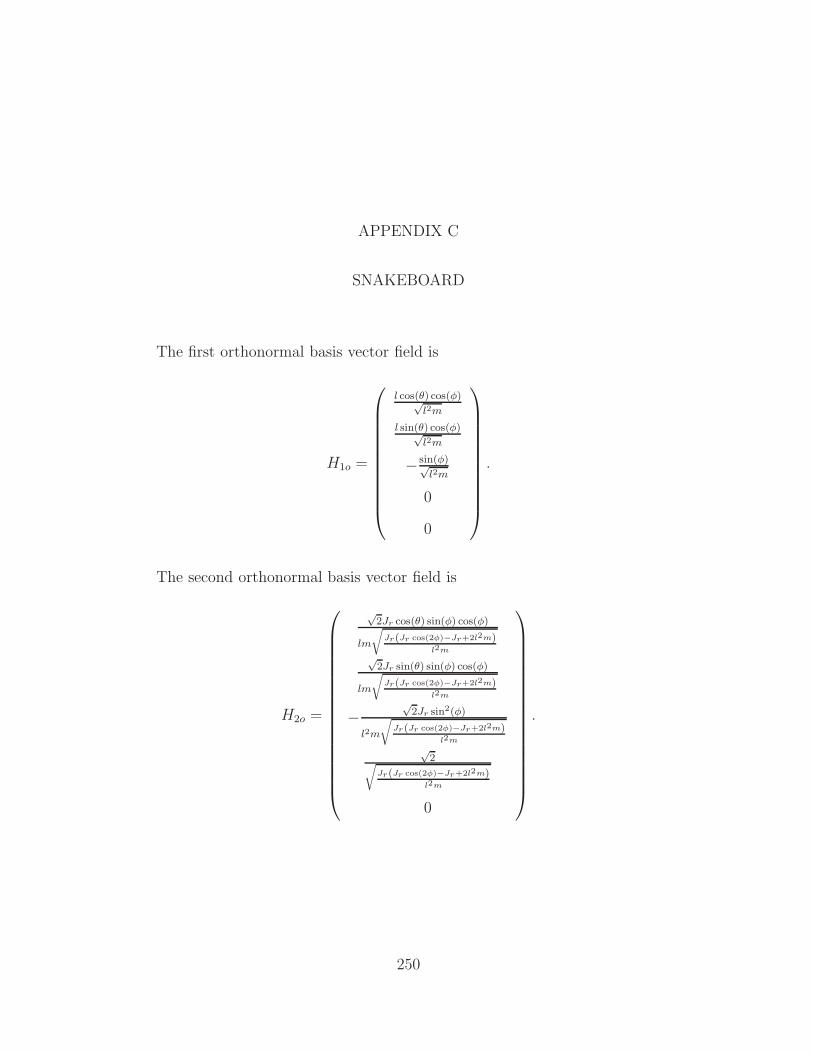
APPENDIX C: SNAKEBOARD . . . . . . . . . . . . . . . . . . . . . . . 250
APPENDIX D: THREE LINK MANIPULATOR . . . . . . . . . . . . . . 253
BIBLIOGRAPHY . . . . . . . . . . . . . . . . . . . . . . . . . . . . . . . 255
v
Page 9
FIGURES
1.1 A schematic of the planar ice skater. . . . . . . . . . . . . . . . . 2
3.1 A schematic of the forced planar rigid body. . . . . . . . . . . . . 84
3.2 A schematic of the roller racer. . . . . . . . . . . . . . . . . . . . 86
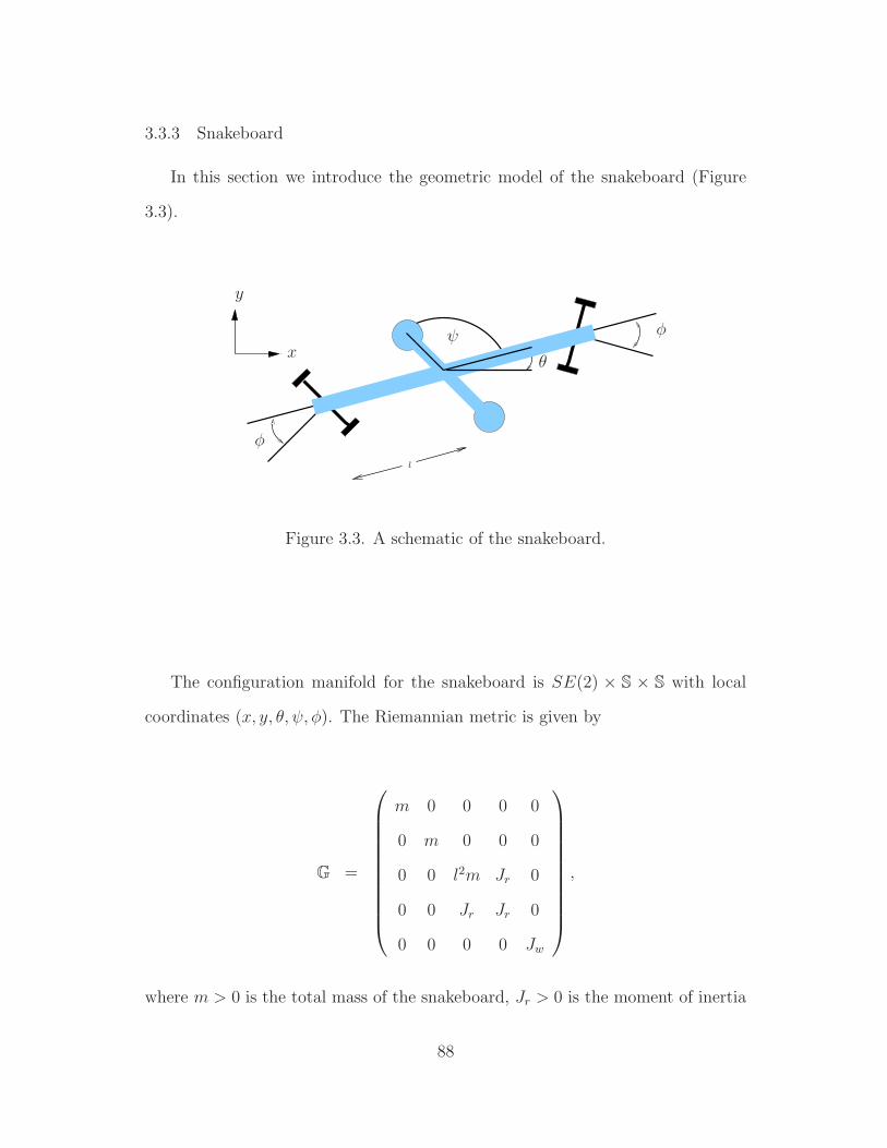
3.3 A schematic of the snakeboard. . . . . . . . . . . . . . . . . . . . 88
3.4 A schematic of the three link manipulator. . . . . . . . . . . . . . 90
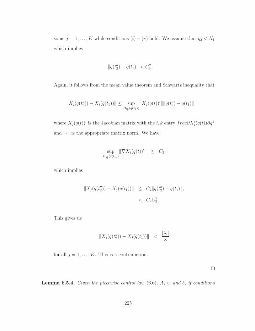
6.1 A simulation of the velocity to velocity algorithm for the planarrigid body. In each subplot, the trajectory of the velocity compo-nent is a solid line and the target velocity is a dashed line. PlotA displays the unactuated velocity component being driven froms(t0) = −15 to s(T ) = 0. Plot B displays the first actuated velocitycomponent being driven from w1(t0) = 25 to w1(T ) = 0. Plot Cdisplays the second actuated velocity component being driven fromw2(t0) = −10 to w2(T ) = 0. Note that the instantaneous changein slope found in Plot B and C corresponds to switching betweenstages in the control law. . . . . . . . . . . . . . . . . . . . . . . 231
6.2 A simulation of the velocity to velocity algorithm for the planarrigid body. Plot A displays the unactuated velocity componentbeing driven from s(t0) = −15 to s(T ) = −25. Plot B displaysthe first actuated velocity component being driven from w1(t0) =25 to w1(T ) = 10. Plot C displays the second actuated velocitycomponent being driven from w2(t0) = −10 to w2(T ) = 20. . . . 232
6.3 A simulation of the velocity to velocity algorithm for the planarrigid body. Plot A displays the unactuated velocity componentbeing driven from s(t0) = −15 to s(T ) = 5. Plot B displays thefirst actuated velocity component being driven from w1(t0) = 5 tow1(T ) = 10. Plot C displays the second actuated velocity compo-nent being driven from w2(t0) = −10 to w2(T ) = −10. . . . . . . 234
vi
Page 10
6.4 A simulation of the velocity to velocity algorithm for the planarrigid body. Plot A displays the unactuated velocity componentbeing driven from s(t0) = 15 to s(T ) = 0. Plot B displays the firstactuated velocity component being driven from w1(t0) = −10 tow1(T ) = 0. Plot C displays the second actuated velocity componentbeing driven from w2(t0) = 20 to w2(T ) = 0. . . . . . . . . . . . 235
6.5 A simulation of the velocity to velocity algorithm for the rollerracer. Plot A displays the unactuated velocity component beingdriven from s(t0) = 15 to s(T ) = 0. Plot B displays the actuatedvelocity component being driven from w1(t0) = 5 to w1(T ) = 0. . 236
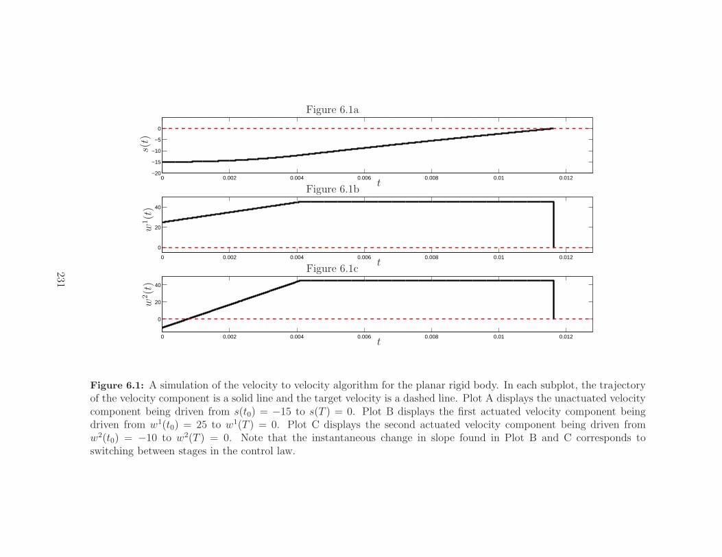
6.6 A simulation of the velocity to velocity algorithm for the snake-board. Plot A displays the unactuated velocity component be-ing driven from s(t0) = −15 to s(T ) = 5. Plot B displays thefirst actuated velocity component being driven from w1(t0) = 5 tow1(T ) = 10. Plot C displays the second actuated velocity compo-nent being driven from w2(t0) = −10 to w2(T ) = 20. . . . . . . . 238
6.7 A simulation of the velocity to velocity algorithm for the snake-board. Plot A displays the unactuated velocity component be-ing driven from s(t0) = −15 to s(T ) = 0. Plot B displays thefirst actuated velocity component being driven from w1(t0) = 5 tow1(T ) = 0. Plot C displays the second actuated velocity componentbeing driven from w2(t0) = −10 to w2(T ) = 0. . . . . . . . . . . . 239
6.8 A simulation of the velocity to velocity algorithm for the three link
manipulator. Plot A displays the unactuated velocity component being
driven from s(t0) = 5 to s(T ) = −6. Plot B displays the first actuated
velocity component being driven from w1(t0) = 5 to w
1(T ) = 10. Plot
C displays the second actuated velocity component being driven from
w2(t0) = −10 to w
2(T ) = 20. . . . . . . . . . . . . . . . . . . . . . 2406.9 A simulation of the velocity to velocity algorithm for the three link
manipulator. Plot A displays the unactuated velocity componentbeing driven from s(t0) = 5 to s(T ) = 0. Plot B displays thefirst actuated velocity component being driven from w1(t0) = 5 tow1(T ) = 0. Plot C displays the second actuated velocity componentbeing driven from w2(t0) = −10 to w2(T ) = 0. . . . . . . . . . . 241
vii
Page 11
ACKNOWLEDGMENTS
I wish to express my sincere appreciation to the Department of Aerospace and
Mechanical Engineering and Department of Mathematics for their extended long-
term support and especially to my advisors Professor Bill Goodwine and Professor
Richard Hind for their patience, encouragement and knowledge. This thesis would
never have been completed without the love, devotion and inspiration of my wife,
Alice. Thank you for always believing in me. I am truly blessed.
viii
Page 12
CHAPTER 1
INTRODUCTION
Mechanics and control theory are two well developed fields of study. Howev-
er, their intersection still provides a rich and challenging research area commonly
referred to as geometric control of mechanical systems. Underactuat-
ed mechanical systems or mechanical control systems with fewer actuators than
degrees of freedom form a large and important subclass. Whenever fewer input
forces are available than degrees of freedom, various control questions arise. The
linear approximation around equilibrium points may, in general, not be control-
lable. These systems require fundamental nonlinear approaches. The areas of
application of control theory for underactuated mechanical systems are diverse
and challenging. Such areas include autonomous aerospace and marine vehicles,
robotics, mobile robots, constrained systems and legged locomotion. The formal-
ism of linear connections and distributions on a Riemannian manifold provides an
elegant framework for modeling, analysis and control Lewis [42].
1.1 Motivating Example
As a concrete example, take the planar ice skater illustrated in Figure 1.1.
The schematic drawing illustrates the kinematics and actuator locations of the
model. Note that each leg is composed of two links which are connected by
1
Page 13
(x, y)
γ1
γ2
θb
B1
B2
X
Y
d1
d2
Figure 1.1. A schematic of the planar ice skater.
a translation joint at the knee and a pin joint at the hip. The foot is an ice
skate which is constrained to the plane in such a way that prohibits motion of
the foot perpendicular to the blade. Technically speaking, the skate blade forms a
nonholonomic constraint with the plane and gives rise to interesting geometries
that can be modeled using the affine connection formalism.
A single actuator capable of generating torque in both the clockwise and coun-
terclockwise directions is placed at each pin joint or hip. Another set of linear
actuators are placed at each translation joint or knee. The planar ice skater has
five degrees of freedom and only four actuators. This is an example of an un-
deractuated control system. Unactuated states give rise to many interesting
control questions. For instances, it is not immediately clear whether the mov-
ing ice skater can be “stopped” using the limited control authority. If it cannot
be stopped, then the set of reachable velocities does not include zero velocity. In
this, and other underactuated mechanical systems, existing geometric control theo-
ry does not provide a general test for stopping and more generally speaking, the set
2
Page 14
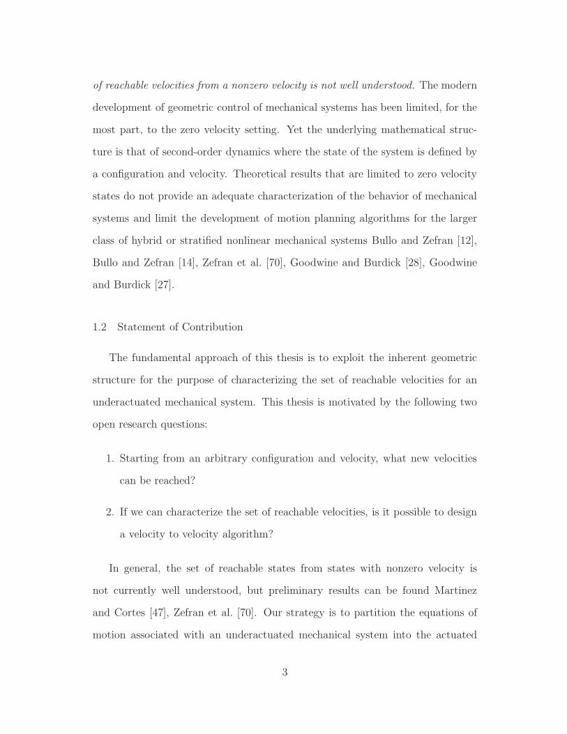
of reachable velocities from a nonzero velocity is not well understood. The modern
development of geometric control of mechanical systems has been limited, for the
most part, to the zero velocity setting. Yet the underlying mathematical struc-
ture is that of second-order dynamics where the state of the system is defined by
a configuration and velocity. Theoretical results that are limited to zero velocity
states do not provide an adequate characterization of the behavior of mechanical
systems and limit the development of motion planning algorithms for the larger
class of hybrid or stratified nonlinear mechanical systems Bullo and Zefran [12],
Bullo and Zefran [14], Zefran et al. [70], Goodwine and Burdick [28], Goodwine
and Burdick [27].
1.2 Statement of Contribution
The fundamental approach of this thesis is to exploit the inherent geometric
structure for the purpose of characterizing the set of reachable velocities for an
underactuated mechanical system. This thesis is motivated by the following two
open research questions:
1. Starting from an arbitrary configuration and velocity, what new velocities
can be reached?
2. If we can characterize the set of reachable velocities, is it possible to design
a velocity to velocity algorithm?
In general, the set of reachable states from states with nonzero velocity is
not currently well understood, but preliminary results can be found Martinez
and Cortes [47], Zefran et al. [70]. Our strategy is to partition the equations of
motion associated with an underactuated mechanical system into the actuated
3
Page 15
and unactuated dynamics. This partitioning gives rise to an intrinsic symmetric
bilinear form that represents the coupling between the actuated and unactuated
velocity states. We use the definiteness of the intrinsic symmetric bilinear form
as sufficient conditions for a general test for velocity reachability. We focus on a
constructive solution that naturally gives rise to a velocity to velocity algorithm.
This thesis contains contributions to modeling, analysis and algorithm design for
underactuated mechanical systems.
We provide two novel differential geometric formulations of the nonlinear con-
trol models for underactuated mechanical control systems. It is well-known that
the choice of representation for mechanical control systems can be a key step
in confronting any problem. For example, mechanical control systems with con-
straints can be described by a coordinate-invariant affine connection Lewis [41].
The coordinate-invariant model is elegant and provides a natural link to previous
results for unconstrained mechanical systems Lewis and Murray [44]. However,
the explicit representation of the so-called constrained affine connection requires
cumbersome differentiation of a tensor field. An alternative representation was
developed a few years later Bullo and Zefran [13]. This simplification led to a
more efficient method of computing and ultimately interpreting the Christoffel
symbols of the connection. The Christoffel symbols play an important role in
computing symmetric products which are used to characterize the structure of
the accessibility distribution at zero velocity. The accessibility distribution can
then be used to characterize the reachable set of velocities and configurations.
The key feature shared by both of our formulations is the partitioning of the
equations of motion into the actuated and unactuated dynamics. Both formula-
tions are constructed using control forces and the kinetic energy metric inherent
4
Page 16
in the classic problem formulation. Interestingly, each formulation gives rise to an
intrinsic vector-valued quadratic (symmetric bilinear) form that can be associat-
ed with an underactuated mechanical control system. The following subsections
detail each contribution of this thesis.
1.2.1 Affine Foliation for Underactuated Mechanical Systems
We develop an alternative representation of the equations of motion for the
general class of underactuated mechanical systems by constructing an affine fo-
liation of the tangent bundle. We use the Riemannian metric along with the
control forces to construct an orthonormal frame on the tangent bundle using the
input distribution Y and the Riemannian metric G included in the basic problem
formulation. Though Riemannian geometry is a classic technique in modeling un-
deractuated mechanical systems, affine foliations and affine subbundles are not.
In general, we think of an underactuated mechanical system as moving from leaf
to leaf in the affine foliation. Each leaf in the affine foliation is parameterized by
a family of one-forms referred to as the affine parameters. We will show that the
affine parameters represent the unactuated velocity states. Each leaf in the affine
foliation can also be associated with an affine subbundle. The linear part of the
affine subbundle is parameterized by a second family of one-forms referred to as the
linear parameters. We will show that the linear parameters represent the actuated
velocity states. We demonstrate that the characterization of the affine parame-
ters along system trajectories correspond to the unactuated dynamics while the
characterization of the linear parameters along system trajectories correspond to
the actuated dynamics. Our modeling leads to two important observations. First,
the actuated dynamics can be linearized using partial feedback linearization. This
5
Page 17
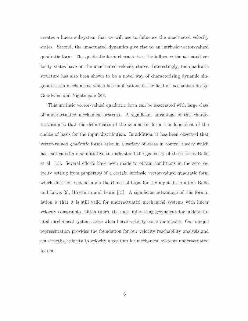
creates a linear subsystem that we will use to influence the unactuated velocity
states. Second, the unactuated dynamics give rise to an intrinsic vector-valued
quadratic form. The quadratic form characterizes the influence the actuated ve-
locity states have on the unactuated velocity states. Interestingly, the quadratic
structure has also been shown to be a novel way of characterizing dynamic sin-
gularities in mechanisms which has implications in the field of mechanism design
Goodwine and Nightingale [29].
This intrinsic vector-valued quadratic form can be associated with large class
of underactuated mechanical systems. A significant advantage of this charac-
terization is that the definiteness of the symmetric form is independent of the
choice of basis for the input distribution. In addition, it has been observed that
vector-valued quadratic forms arise in a variety of areas in control theory which
has motivated a new initiative to understand the geometry of these forms Bullo
et al. [15]. Several efforts have been made to obtain conditions in the zero ve-
locity setting from properties of a certain intrinsic vector-valued quadratic form
which does not depend upon the choice of basis for the input distribution Bullo
and Lewis [9], Hirschorn and Lewis [31]. A significant advantage of this formu-
lation is that it is still valid for underactuated mechanical systems with linear
velocity constraints. Often times, the most interesting geometries for underactu-
ated mechanical systems arise when linear velocity constraints exist. Our unique
representation provides the foundation for our velocity reachability analysis and
constructive velocity to velocity algorithm for mechanical systems underactuated
by one.
6
Page 18
1.2.2 Partitioning Connections for Underactuated Mechanical Systems
A common starting point for treatments of underactuated mechanical systems
is to assume that there exists a set of coordinates q = (q1, . . . , qn) such that the
local expression for the governing equations of motion are
M11(q)q1 +M12(q)q2 + F1(q, q) = B(q)u (1.1)
M21(q)q1 +M22(q)q2 + F2(q, q) = 0 (1.2)
where q1 ∈ Rm is the first m-components of q ∈ Rn and represents the actuated
degrees of freedom, q2 ∈ Rn−m is the remaining n−m-components of q ∈ Rn and
represents the unactuated degrees of freedom, and Mij(q) represents n×n inertia
matrix Spong [59], Reyhanoglu et al. [57], Olfati-Saber [53]. The basic idea is that
only the first m degrees of freedom are actuated. Equation (1.1) represents the
actuated dynamics, while Equation (1.2) represents the unactuated dynamics. A
known limitation of this formulation for underactuated mechanical systems is that
it requires that the input codistribution to be integrable Bullo and Lewis [10]. It
is not always physically valid to assume that the input codistribution is integrable
for a general underactuated mechanical system. Many of the mechanical systems
considered in this body of research have a single actuator which always gives rise to
integrable codistributions. For example, the forced planar rigid body and various
constrained systems considered in this thesis do not satisfy this assumption.
This thesis contains an alternative formulation for underactuated mechanical
systems that utilizes partitioning connections. We introduce two linear connec-
tions that provide a coordinate invariant representation that partitions the actu-
ated and unactuated dynamics. Our formulation does not require that the input
7
Page 19
codistribution be integrable, therefore can be viewed as a generalization of the par-
titioning used in existing literature on underactuated mechanical systems Spong
[59], Reyhanoglu et al. [57], Olfati-Saber [53]. We show that feedback linearization
of the actuated dynamics gives rise to a control-affine system whose drift vector
field is the geodesic spray of the unactuated connection associated with unactu-
ated dynamics. We call this control-affine system the geometric normal form for
underactuated mechanical systems. The geometric normal form is the starting
point for our reachability analysis and motion algorithms for mechanical systems
underactuated by one. Similar to the affine foliation formalism, the unactuated
connection gives rise to an intrinsic vector-valued symmetric bilinear (quadrat-
ic) form. Again, a significant advantage of the partitioning connections is that
the formulation is still valid for the extended class of underactuated mechanical
systems with linear velocity constraints.
1.2.3 Characterization of Reachable Velocities for Mechanical Systems Underac-
tuated by One
One of the fundamental problems in control theory is determining the set of
states reachable from an initial state. Problems of this nature are commonly re-
ferred to as controllability. A detailed review of controllability and existing results
for underactuated mechanical systems can be found in Section 1.3. The matter
of determining the general structure of states reachable from a nonzero velocity
state is currently unresolved Bullo and Lewis [10], Cortes et al. [21], Bullo and Ze-
fran [14]. We provide a general test for mechanical systems underactuated by one
control that depends on the definiteness of an intrinsic symmetric bilinear form
that determines the system’s ability to reach a specified velocity from a nonzero
8
Page 20
velocity state. In other words, we provide a sufficient condition dependent on
the definiteness of a symmetric bilinear form for velocity to velocity motion plan-
ning. A significant advantage of our result is that it applies to mechanical systems
underactuated by one control with linear velocity constraints. Underactuated me-
chanical systems with linear velocity constraints give rise to nontrivial geometries
that are challenging to analyze and control. Here is an informal statement of our
main result.
Theorem 1.2.1 (Reachability for Mechanical Systems Underactuated by One
Control). Consider a mechanical system underactuated by one control (possibly
with linear velocity constraints) whose intrinsic symmetric bilinear form is indef-
inite at the given configuration and velocity. For any ǫ, α,∆ > 0 and any target
velocity there exists a piecewise control law that will drive the system to any ǫ-ball
of the target velocity in time less than ∆ while staying within an α-ball of the
initial configuration.
Though our main result can be applied to nonzero velocity targets, we also
consider the problem of reaching rest which can be viewed as a form of stabiliza-
tion. This test is applicable to both constrained and unconstrained systems. Here
is the statement of our corollary for stopping.
Corollary 1.2.2 (Stopping for Mechanical Systems Underactuated by One Con-
trol). Consider a mechanical system underactuated by one control (possibly with
linear velocity constraints) whose intrinsic symmetric bilinear form is indefinite at
the given configuration and velocity. For any ǫ, α,∆ > 0 there exists a piecewise
control law that will drive the system to any ǫ-ball of rest in time less than ∆ while
staying within an α-ball of the initial configuration.
9
Page 21
Our theoretical results are useful for two reasons. First, such results are neces-
sary conditions for velocity to velocity motion algorithms. In terms of stopping, if
zero velocity is not contained in the set of reachable velocities, then it is impossible
to specify a control law that will drive the system to rest. Second, these results
are useful design tools which provide constructive strategies for actuator assign-
ment and help to make the control scheme robust to actuator failure Tafazoli [65].
The task of actuator assignment is always a balance between the sophistication
of the system design and the associated complexity of the controller. For exam-
ple, a system which is fully actuated requires a simple control scheme to drive it
to rest. In contrast, if the system is underactuated even by just one control, a
control scheme must take into account the underlying geometry or nonlinearities
of the geometric model. Such a control scheme is theoretically challenging due to
nonzero drift which indicates a component of the dynamics that is not directly
controlled or unactuated.
There has been preliminary work done on stopping underactuated mechanical
systems. It has been shown that the roller racer and the robotrikke could not be
stopped given a single control input from an arbitrary initial configuration and
velocity Krishnaprasad and Tsakiris [37], Chitta et al. [18]. It is important to note
that the existing investigations into the roller racer and robotrikke have focused
on a particular instance of a mechanical system underactuated by one control and
cannot be easily extended to different systems in the same class. Further, we show
that given certain conditions on the symmetric bilinear form and the relationship
between the initial unactuated velocity state and the targeted velocity state that
the roller racer can be driven arbitrarily close to rest.
It is true that nonlinear mechanical systems underactuated by one control is
10
Page 22
the simplest case next to fully actuated systems. However, these systems are not
feedback linearizable and thus not amendable to standard techniques in control
theory Isidori [33]. The literature on the analysis and control of mechanical sys-
tems underactuated by one control is vast. Such systems include underactuated
ships Do [23], gymnastic robots Xin and Kaneda [68], the Harrier which is a planar
vertical/short take-off and landing (V/STOL) aircraft in the absence of gravity
Sastry [58], a hovercraft type vehicle Tanaka et al. [66] and a planar rigid body
with two thrusters moving on a flat horizontal plane M’Closkey [48].
1.2.4 Velocity to Velocity Algorithm for Mechanical Systems Underactuated by
One
The problem of general motion planning for underactuated mechanical sys-
tems is still not well understood Martinez and Cortes [47], Bullo and Lewis [10].
Due to the challenging nature of these problems, many of the existing results have
been limited for example to gait generation algorithms applicable only to the
specific systems Ostrowski et al. [55], Chitta and Kumar [17], Chitta et al. [18],
configuration to configuration algorithms with zero-velocity transitions between
feasible motions for specific systems Bullo and Lewis [8], Bullo and Zefran [14]
and numerically generated optimal trajectories J.P. Ostrowski and Kumar [56].
In contrast, we demonstrate the utility of our alternative formulations and sym-
metric bilinear form by constructing a general velocity to velocity algorithm. The
algorithm is a natural consequence of the constructive proof of our main result on
velocity reachability. The use of the intrinsic symmetric form as a constructive
tool for motion algorithms for underactuated mechanical systems in this thesis is
a new contribution to existing control literature, although preliminary results can
11
Page 23
be found in Nightingale et al. [51], Nightingale et al. [50], Nightingale et al. [49].
Illustrative examples of the control algorithm can be found in Chapter 6.
1.3 Literature Review
This thesis has been inspired by a differential geometric approach to control
theory. Here we review the role that geometry has played in the development of
control theory and the influence it has had on modeling, analysis and control of
mechanical systems.
In general, control theory is the study of the manipulation of a dynamical
system in order to obtain a desired objective. The dynamical laws governing these
systems are not fixed as in classical physics, rather they depend on parameters
referred to as controls. Roughly speaking, a “mechanical control system” is a
system of second-order differential equations defined on the tangent bundle of the
configuration manifold in which the control function appears as parameters. An
important geometric observation is that the natural dynamics (geodesic spray)
and each control (external force) determines a vector field on the tangent bundle,
and thus a mechanical control system can be viewed as a family of vector fields on
the tangent bundle some of which are parameterized by controls. A trajectory of
such a system is a continuous curve made up of finitely many segments of integral
curves of the vector fields in the family.
The formalism of affine connections and distributions (geometric) have been
shown to provide an adequate geometric framework for modeling, analysis and
control given zero initial velocity Bullo and Lewis [10]. If the initial velocity of
the control system is zero, then we may associate the family of vector fields with
a distribution. The distribution can then be used to derive controllability results.
12
Page 24
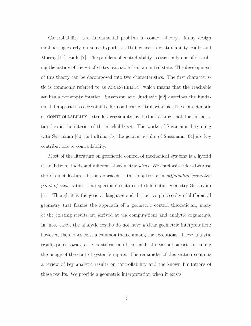
Controllability is a fundamental problem in control theory. Many design
methodologies rely on some hypotheses that concerns controllability Bullo and
Murray [11], Bullo [7]. The problem of controllability is essentially one of describ-
ing the nature of the set of states reachable from an initial state. The development
of this theory can be decomposed into two characteristics. The first characteris-
tic is commonly referred to as accessibility, which means that the reachable
set has a nonempty interior. Sussmann and Jurdjevic [62] describes the funda-
mental approach to accessibility for nonlinear control systems. The characteristic
of controllability extends accessibility by further asking that the initial s-
tate lies in the interior of the reachable set. The works of Sussmann, beginning
with Sussmann [60] and ultimately the general results of Sussmann [64] are key
contributions to controllability.
Most of the literature on geometric control of mechanical systems is a hybrid
of analytic methods and differential geometric ideas. We emphasize ideas because
the distinct feature of this approach is the adoption of a differential geometric
point of view rather than specific structures of differential geometry Sussmann
[61]. Though it is the general language and distinctive philosophy of differential
geometry that frames the approach of a geometric control theoretician, many
of the existing results are arrived at via computations and analytic arguments.
In most cases, the analytic results do not have a clear geometric interpretation;
however, there does exist a common theme among the exceptions. These analytic
results point towards the identification of the smallest invariant subset containing
the image of the control system’s inputs. The remainder of this section contains
a review of key analytic results on controllability and the known limitations of
these results. We provide a geometric interpretation when it exists.
13
Page 25
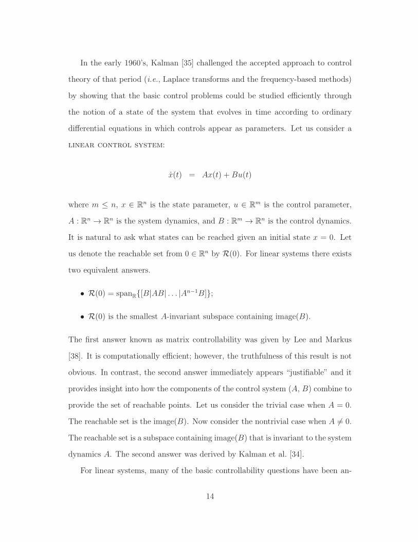
In the early 1960’s, Kalman [35] challenged the accepted approach to control
theory of that period (i.e., Laplace transforms and the frequency-based methods)
by showing that the basic control problems could be studied efficiently through
the notion of a state of the system that evolves in time according to ordinary
differential equations in which controls appear as parameters. Let us consider a
linear control system:
x(t) = Ax(t) +Bu(t)
where m ≤ n, x ∈ Rn is the state parameter, u ∈ R
m is the control parameter,
A : Rn → Rn is the system dynamics, and B : Rm → Rn is the control dynamics.
It is natural to ask what states can be reached given an initial state x = 0. Let
us denote the reachable set from 0 ∈ Rn by R(0). For linear systems there exists
two equivalent answers.
• R(0) = spanR{[B|AB| . . . |An−1B]};
• R(0) is the smallest A-invariant subspace containing image(B).
The first answer known as matrix controllability was given by Lee and Markus
[38]. It is computationally efficient; however, the truthfulness of this result is not
obvious. In contrast, the second answer immediately appears “justifiable” and it
provides insight into how the components of the control system (A, B) combine to
provide the set of reachable points. Let us consider the trivial case when A = 0.
The reachable set is the image(B). Now consider the nontrivial case when A 6= 0.
The reachable set is a subspace containing image(B) that is invariant to the system
dynamics A. The second answer was derived by Kalman et al. [34].
For linear systems, many of the basic controllability questions have been an-
14
Page 26
swered. The matter of providing general conditions for determining the structure
of the reachable set for a general nonlinear control system is currently unresolved,
however there have been many deep and insightful contributions.
In 1963, Hermann [30] related Chow’s theorem [19] to control theory. Let us
consider the following driftless nonlinear system:
x(t) = u1(t)g1(x) + · · · + um(t)gm(x)
where x ∈ M is the state parameter, M is a smooth manifold, u : R → Rm is
the control parameter, and {g1, . . . , gm} is a family of control vector fields on M .
Loosely speaking, the family of vector fields can be associated with a distribution
D on M . A distribution D on M is a smooth assignment of a subspace Dx, for
each x ∈M , of the tangent space TxM . Chow’s theorem implies that the closure
of the distribution D under the Lie bracket, denoted by Lie(∞)(D), is the smallest
invariant subspace of the tangent space containing the image(D). Provided that
the set of inputs u satisfy certain restrictions, the geometric interpretation is
that the reachable set is the submanifold S ⊂ M such that TxS = Lie(∞)(D)
for each x ∈ M . The driftless control system is small-time locally controllable if
TxM = Lie(∞)(D) for each x ∈M .
The most general class of nonlinear control systems presented in this thesis is
commonly referred to as control-affine systems. The problem of determining
controllability for underactuated control-affine systems is difficult. Let us consider
the following control-affine system:
x(t) = f(x) + u1(t)g1(x) + · · · + um(t)gm(x)
15
Page 27
where x ∈M is the state parameter, M is a smooth manifold, u : R → Rm is the
control parameter, f is the drift vector field on M , and {g1, . . . , gm} is a family
of control vector fields on M . The extreme challenge of deriving controllability
conditions for this class of nonlinear control systems is a consequence of the drift
vector field. The drift vector field represents system dynamics that are not pa-
rameterized by controls or unactuated dynamics. As mentioned earlier, Sussmann
and Jurdjevic [62] have characterized the fundamental approach to accessibility
for control-affine systems. It is the case that accessibility for control-affine sys-
tems has a geometric interpretation in the context of orbits. In contrast, local
controllability for control-affine systems has only been characterized analytically.
Sussmann [64] provides sufficient conditions for small-time local controllability
for control-affine systems that follow a Lie series approach which incorporates the
ideas of Crouch and Byrnes [22] concerning input symmetries. The formal proof
employs the use of free Lie algebras. Note that a detailed statement of these results
requires the introduction of a significant amount of notation that the uninitiated
reader can expect to devote some time to understanding due to the use of free Lie
algebras. There are three well-known limitations to the results by Sussmann [64]:
1. The general sufficient conditions for local controllability of a control-affine
system are restricted to an equilibrium point.
2. The general conditions are dependent upon the choice of basis for the input
distribution and thus sufficient.
3. The general sufficient conditions for local controllability of a control-affine
system gives rise to a geometric growth in the number of elements to test.
Despite these limitations, Sussmann’s work [64] on sufficient conditions for small-
16
Page 28
time local controllability forms the cornerstone of many existing analyzes of me-
chanical control systems. In contrast to the vast majority of literature on control-
lability for underactuated mechanical systems, this thesis is not an application of
the results of Sussmann [64].
Let us consider the following mechanical control system:
Ψ′(t) = Z(v) + u1(t)Y vlft1 (v) + · · · + um(t)Y vlft
m (v)
where Ψ ∈ TM is the state parameter, TM is the tangent bundle, u : R → Rm
is the control parameter, Z is the geodesic spray of the Levi-Civita connection or
drift vector field on TM , and {Y vlft1 , . . . , Y vlft
m } is a family of control vector fields
on M vertically lifted to TM . A mechanical control system can be identified with
a control-affine system on TM , and thus the results of Sussmann [64] on con-
trollability will apply. However, mechanical control systems carry an additional
metric or connection structure which simplifies their analysis. Lewis and Murray
[44] study this class of nonlinear control systems because their unique structure
had been underexploited in literature. Relying on the results of Sussmann [64],
Lewis and Murray [44] provide computable sufficient conditions for small-time
configuration controllability for a class of mechanical systems. Configu-
ration controllability is strictly concerned with the reachable set of configuration
states and not velocity states. Lewis and Murray [44] focus on simple mechani-
cal systems, which forms an important subset of all mechanical systems. Simple
mechanical systems are characterized by the Lagrangian equal to the difference
between kinetic energy and potential energy. Note that the results obtained by
Lewis and Murray [44] inherited the limitations associated with the original work
Sussmann [64]. However, Lewis and Murray [44] were able to show that the ge-
17
Page 29
ometric growth in the number of elements to test can be pruned by using the
unique Riemannian or affine connection structure associated with simple mechan-
ical systems. There are two key features associated with the results of Lewis and
Murray [44]:
1. The general sufficient conditions for accessibility and small-time local con-
trollability of simple mechanical control systems is limited to initial states
with zero velocity.
2. The general conditions are dependent upon the choice of basis for the input
distribution and thus sufficient.
These results were extended by Lewis [41] to affine connection control systems
with constraints and used to provide a decomposition for affine connection control
systems Lewis and Murray [43]. Affine connection control systems form a subclass
of simple mechanical systems where the Lagrangian is strictly kinetic energy Bullo
and Lewis [10]. Finally, the results of Lewis and Murray [44] have been extended
to affine connection control systems with dissipation Cortes et al. [20] and to
the larger class of simple mechanical control systems (i.e., nonzero potential)
with dissipation Kang et al. [36]. Note that each of these extensions inherit the
limitations of the original results Sussmann [64] and are restricted to initial states
with zero velocity.
Let us return to the second limitation of Sussmann [64]. It implies that the
conditions are not invariant under input transformations. The consequences of the
lack of feedback invariance can be seen even in simple examples, where the system
can fail the sufficient condition test, but still be controllable. This indicates the
need to develop controllability tests independent of the choice of basis for the in-
put distribution. There have been several attempts to sharpen the configuration
18
Page 30
controllability results using the Riemannian or affine connection structure associ-
ated with mechanical systems. Lewis [39] investigated the single-input case from
rest, building on previous results for general scalar-input systems Sussmann [63].
However, mechanical control systems with a single-input are special cases.
The results of Lewis and Murray Lewis and Murray [44] provide an analytic
description of the reachable set. The geometric interpretation of the reachable
set was obtained by Lewis [40] at a later date. Lewis [40] introduces the notion
of a geodesically invariant distribution and provides a product of vector
fields (symmetric product) which allows one to test for geodesic invariance in the
same way one uses the Lie bracket to test for integrability. A distribution D
is geodesically invariant if and only if D ⊂ TM is invariant under the geodesic
flow. Geometrically, a geodesically invariant distribution plays the same role in
interpreting the reachable set that the “smallest A-invariant subspace containing
the image(B)” does for linear control systems. Loosely speaking, the geodesically
invariant distribution D is a distribution on the tangent bundle of the phase
manifold and represents all possible velocities that can be reached from rest. The
identification of this invariant distribution was the key insight into the geometric
interpretation of the reachable set for affine connection control systems.
This thesis is most closely related to the work of Bullo and Lewis [8],Hirschorn
and Lewis [31], Tyner and Lewis [67],Hirschorn and Lewis [32],Bullo et al. [15].
These papers mark a shift in literature towards a geometric, rather than analyt-
ic, investigation into properties of local controllability. Hirschorn and Lewis [31]
study the basic geometric properties of local controllability for control-affine sys-
tems. They contend that in a geometric point of view, a nonlinear control system,
affine in the controls, can be thought of as an affine subbundle of the tangent
19
Page 31
bundle of the state space. Further, Hirschorn and Lewis [31] derive geometric
conditions dependent upon the properties of the affine subbundle that either en-
sure or prohibit local controllability. These results are limited to second-order
conditions and affine subbundles containing zero velocity. The advantage of this
approach, at least for low-order controllability, is that the conditions are indepen-
dent of the basis representing the input distribution. The controllability results
by Bullo and Lewis [8] bear strong resemblance to the more general conditions of
Hirschorn and Lewis [31]. However, Bullo and Lewis [8] are able to provide more
detail in this case because they restrict their attention to affine connection control
systems. They obtain low-order controllability results using a certain intrinsic
vector-valued quadratic form that can be associated to an affine connection con-
trol system. Additional uses of vector-valued quadratic forms in control theory
are outlined by Bullo et al. [15].
1.4 Outline of Thesis
A brief outline of the content of the various chapters is as follows:
Chapter 1. Here we provide a motivating example, statement of the contribu-
tions and literature review.
Chapter 2. Here we review necessary tools from differential geometry and Rie-
mannian geometry. We include numerous local coordinate expressions that
are required to analyze and numerical simulate specific examples.
Chapter 3. Here we review the formulation of mechanical control systems on
Riemannian manifolds.
Chapter 4. Here we present the first modeling contribution of this thesis. We
20
Page 32
construct an affine foliation of the tangent bundle for underactuated me-
chanical systems. We use the affine foliation to partition the actuated and
unactuated dynamics. We provide a characterization of an underactuated
mechanical systems ability to move from leaf to leaf in the affine foliation.
Chapter 5. Here we present the second modeling contribution of this thesis. We
construct two partitioning connections for underactuated mechanical sys-
tems. We use the two connections to partition the actuated and unactuated
dynamics. We also introduce a partial feedback linearization control law
that gives rise to our geometric normal form. The geometric normal form
serves as a starting point for our reachability analysis and velocity to velocity
algorithm.
Chapter 6. Here we present the main analytical contribution of this thesis. We
provide a unique characterization of the reachable set of velocities from an
arbitrary initial configuration and velocity that depends on the definiteness
of an intrinsic symmetric bilinear form. A natural consequence of the con-
structive proof of our main result is a velocity to velocity algorithm. The
algorithm is applied to the forced planar rigid body, roller racer, snakeboard
and three link manipulator. Numerical simulations are included to illustrate
the velocity to velocity algorithm.
Chapter 7. Here we make concluding remarks and state possible directions of
future research.
21
Page 33
CHAPTER 2
MATHEMATICAL PRELIMINARIES
This thesis examines mechanical control systems in the context of differentiable
manifolds and vector bundles. This chapter contains a review of necessary tools
from differential and Riemannian geometry. For an introduction to linear and
multilinear algebra see Abraham et al. [2]. For an introduction to Riemannian
geometry see Carmo [16], Gallot et al. [24], Boothby [6], Yano and Ishihara [69].
For an introduction to geometric mechanics see Arnold [4], Abraham and Marsden
[1] and Oliva [54].
2.1 Differentiable Manifolds
2.1.1 Topological and Differentiable Structure
A n-dimensional topological manifold M is a set that is locally homeomor-
phic to Euclidean space, i.e., there exists a homeomorphism from an open set of
M to an open set of Rn. A homeomorphism φα is a one-to-one map where φα and
its inverse are continuous. A pair (Uα, φα) is called a system of coordinates
or coordinate chart of M at q ∈ M where Uα is an open set of M containing
q and φα is a continuous bijection from Uα to φα(Uα) ⊂ Rn. The homeomor-
phism φα defined on Uα ⊂ M is composed of n local coordinate functions
(x1(q), . . . , xn(q)). For the point q ∈M , the n-tuple (x1, . . . , xn) of φα(q) in Rn is
22
Page 34
called the coordinate of the point q. The local properties of a manifold can be
described by the local coordinate system. We use the coordinate system to write
explicit coordinate-dependent expressions even though the coordinate system itself
has no geometric significance.
In general, it is not possible to cover the whole manifold M with a single
chart. If we need more than one coordinate system {(Uα, φα)} to cover M then
we require that⋃α Uα = M . The collection of opens sets {Uα} is called the open
covering of M . The family of all coordinate charts A = {(Uα, φα)} is called the
atlas of M . If we further require that φα be a smooth bijection that satisfies the
usual compatibility condition then the family {(Uα, φα)} is called a differentiable
structure. In other words, if two open sets Uα and Uβ in the collection of open sets
{Uα} overlap, i.e., Uα∩Uβ 6= 0, then φα◦φ−1β : φβ(Uα∩Uβ) → φα(Uα∩Uβ) must be a
diffeomorphism. The overlap map φα◦φ−1β is a diffeomorphism from φβ(Uα∩Uβ) 7→
φα(Uα ∩ Uβ) if it is a homeomorphism and the map along with its inverse are
smooth. A smooth manifold M is a topological manifold endowed with a C∞
differentiable structure. Intuitively, a manifold’s differentiable structure measures
its smoothness and shows how different open sets in an open covering of the
manifold are patched together.
2.1.2 Tangent Vector, Tangent Space and Tangent Bundle
Let C∞(M) denote the set of all smooth functions f : M → R. Let γ(t) be
a smooth curve through a point q ∈M defined by the map
γ : (−ǫ, ǫ) ⊂ R →M
23
Page 35
where t = 0 is mapped to γ(0) = q. If we restrict f to the smooth curve γ(t) then
we obtain a differentiable function f(γ(t)) with respect to the parameter t. The
rate of change of the function along the curve at point q is given by
d
dtf(γ(t))
∣∣∣∣t=0
.
We define the tangent vector Xq along the curve γ(t) at the point q ∈M to be
the linear differential operator ddt|q that acts on functions along a curve on the
manifold. Tangent vectors defined this way can be thought of as a generalization
of the directional derivative on Rn.
The tangent space TqM to the manifold M is the set of all differential oper-
ators Xq : C∞(M) → R along all curves on the manifold passing through q that
satisfy the Leibniz rule and linearity. Note that TqM is isomorphic to Rn. This
implies that there is a well-defined notion of adding two or more tangent vectors
that live in the same tangent space or multiplying a tangent vector by a real num-
ber. Tangent vectors that live in different tangent spaces cannot be combined or
compared in a natural way. This requires us to either define a one parameter Lie
transformation group or we must introduce additional geometric structure called
a connection.
Let φα(q) = (x1(q), . . . , xn(q)) be the local coordinate functions in the neigh-
borhood Uα ⊂ M containing q. If we take a curve through point q chosen along
the coordinate direction xi, i.e. xi = t, then the rate of change of a function f
along the coordinate curve at point q is
d
dtf(xi(t))
∣∣∣∣t=0
.
24
Page 36
We can expand this expression by applying the chain rule to get
d
dtf(xi(t))
∣∣∣∣t=0
=∂f
∂xi
∣∣∣∣q
∂xi
∂t
∣∣∣∣t=0
.
By definition, we have xi = t which further reduces the expression to
d
dtf(xi(t))
∣∣∣∣t=0
=∂
∂xi
∣∣∣∣q
f.
We see that the tangent vector X iq ∈ TqUα along the coordinate curve xi is ∂
∂xi
∣∣q. In
fact, the tangent vector Xq ∈ TqUα along an arbitrary curve or direction can be ex-
pressed as a linear combination of { ∂∂x1
∣∣q, . . . , ∂
∂xn
∣∣q}. The set { ∂
∂x1
∣∣q, . . . , ∂
∂xn
∣∣q}
is called the local coordinate frame or natural basis for TqUα. Any tangent
vector Xq ∈ TqUα can be written Xq = X i ∂∂xi
∣∣q
where X i ∈ R are called the com-
ponents of Xq with respect to the local coordinate frame. The local expression
for the tangent vector Xq along the curve γ(t) is
f 7→ dγi
dt
∣∣∣∣t=0
∂
∂xi
∣∣∣∣q
f
where γi(t) = xi ◦ γ(t). The components dγi
dt
∣∣∣t=0
of the tangent vector Xq a-
long the curve γ(t) with respect to the local coordinate frame are the velocity
components of γ(t) at t = 0.
The tangent bundle TM is the disjoint union
TM =⋃
q∈MTqM
of all tangent spaces. The tangent bundle is a 2n-dimensional manifold, which is
locally a product manifold. The coordinate charts (Uα, φα) on the manifold M
25
Page 37
give rise to natural charts on the tangent bundle (TUα, Tφα) where
TUα =⋃
q∈Uα
TqUα
and Tφα : TUα → Rn × Rn. The local expression for Tφα is
(q, v) 7→(
(x1(q), . . . , xn(q)),
(∂x1(q)
∂xjvj , . . . ,
∂xn(q)
∂xjvj))
where (v1, . . . , vn) are the components of v with respect to the natural basis for
TqUα. The coordinates for a point (q, v) = vq ∈ TM with respect to the natural
chart on TM will be denoted by ((x1, . . . , xn), (v1, . . . , vn)) ∈ Rn × Rn. The
tangent bundle projection is the map πTM : TM →M defined by πTM(vq) = q
when vq ∈ TqM . The local expression for πTM associated with the natural chart
on TM is
Rn × R
n ∋ ((x1, . . . , xn), (v1, . . . , vn)) 7→ (x1, . . . , xn) ∈ Rn.
2.1.3 Covector, Cotangent Space and Cotangent Bundle
We define the differential of a smooth function f at a point q ∈M to be the
linear map df |q that takes a tangent vector Xq ∈ TqM to R. The differential of
a smooth function df |q is an example of a geometric objected called a covector
ψq. The set of all covectors ψq : TqM → R at the point q on M is called the
cotangent space T ∗qM . Let (Uα, φα) be a coordinate chart on M with the local
coordinate functions (x1(q), . . . , xn(q)) on Uα ⊂M . We can take the differential of
the coordinate functions at a point q ∈ Uα to get the covectors (dx1|q, . . . , dxn|q) ∈
T ∗q Uα. We say that the set of covectors {dx1|q, . . . , dxn|q} are the dual basis to
26
Page 38
{ ∂∂x1
∣∣q, . . . , ∂
∂xn
∣∣q} because dxj |q · ∂
∂xi|q = δji at each point q ∈ Uα where δji is the
Kronecker delta. The Kronecker delta δji is 1 when i and j are equal, and 0
otherwise. The cotangent space is also isomorphic to Rn. Any covector ψq ∈ T ∗q Uα
can be expressed as a linear combination of {dx1|q, . . . , dxn|q} written ψq = ψidxi|q
where ψi ∈ R are components ψq with respect to the dual basis for T ∗q Uα. The
local expression for the differential of a smooth function df |q at a point q ∈ Uα is
C∞(M) ∋ f 7→ ∂f
∂xi
∣∣∣∣q
dxi|q ∈ T ∗q Uα
where ∂f∂xi
|q ∈ R is the component of df |q with respect to the dual basis for T ∗q Uα.
The cotangent bundle T ∗M is the disjoint union
T ∗M =⋃
q∈MT ∗qM
of all cotangent spaces. The cotangent bundle is a 2n-dimensional manifold, which
is locally a product manifold. The coordinate charts (Uα, φα) on the manifold M
give rise to natural charts on the tangent bundle (T ∗Uα, T∗φα) where
T ∗Uα =⋃
q∈Uα
T ∗q Uα
and T ∗φα : T ∗Uα → Rn × Rn. The local expression for T ∗φα is
(q, ψ) 7→(
(x1(q), . . . , xn(q)),
(∂xj(q)
∂x1ψj , . . . ,
∂xj(q)
∂xnψj))
where (ψ1, . . . , ψn) are the components of ψ with respect to the dual basis for T ∗qM .
The coordinates for a point (q, ψ) = ψq ∈ T ∗M with respect to the natural chart
associated with T ∗M will be denoted by ((x1, . . . , xn), (ψ1, . . . , ψn)) ∈ Rn × Rn.
27
Page 39
The cotangent bundle projection is the map πT ∗M : T ∗M → M defined by
πT ∗M(ψq) = q when ψq ∈ T ∗qM . The local expression for πT ∗M associated with the
natural chart on T ∗M is
Rn × R
n ∋ ((x1, . . . , xn), (ψ1, . . . , ψn)) 7→ (x1, . . . , xn) ∈ Rn.
2.1.4 Vector Field, Lie Derivative and Integral Curve
A vector field X on M is a smooth map that associates to each point q ∈M
a tangent vector Xq ∈ TqM . We can also think of X on M as a linear differential
operator that maps
C∞(M) ∋ f 7→ X · f ∈ C∞(M).
We can pair the differential of a smooth function df with X to get a useful object
called the Lie derivative of a function. The Lie derivative of f with respect to
X is defined by the map
q 7→ df(q) ·X(q).
Given the local coordinate function φα(q) = (x1(q), . . . , xn(q)) in the neighborhood
Uα ⊂M containing q, we can define n unique vector fields denoted by ∂∂x1, . . . , ∂
∂xn
on Uα using the Lie derivative of the local coordinate functions with respect to
these vector fields. We define ∂∂xi
to be
L ∂
∂xixj = δji
where i, j ∈ {1, . . . , n} and δij is the Kronecker delta. At each point q ∈ Uα these
vector fields are linearly independent and give rise to the natural basis for TqUα.
We can write X = X i(q) ∂∂xi
for functions X i(q) ∈ C∞(M) called the components
28
Page 40
of X with respect to the chart (Uα, φα). Further, the local expression for the Lie
derivative of a function f with respect to the vector field X denoted by LXf in
the chart (Uα, φα) is
C∞(M) ∋ f 7→ X i(q)∂f
∂xi∈ C∞(M).
Let Γ(TUα) be the set of all smooth vector fields on Uα ⊂ M and Γ(TRn) ≃
Γ(Rn × Rn) be the set of all smooth vector fields on Rn × Rn. Given the natural
chart (Tφα, TUα) on TM , Tφα naturally induces a mapping Tφα : Γ(TUα) →
Γ(TRn) ≃ Γ(Rn × Rn) given by the expression
Γ(TUα) ∋ X i(q)∂
∂xi7→ X i(x1, . . . , xn)ei ∈ Γ(Rn × R
n)
where the set of vectors {e1, . . . , en} is the standard basis for Rn. It follows that
Tφα takes the set of vector fields { ∂∂x1, . . . , ∂
∂xn} into the standard basis on Rn.
Let Γ(TM) be the set of all smooth vector fields on M . The addition of two
or more vector fields is well-defined. In addition, there is a well-defined product
between two vector fields called the Lie bracket. For any X, Y ∈ Γ(TM), the
vector field [X, Y ] defined by
L[X,Y ]f = LXLY f − LYLXf,
is the Lie bracket of X and Y , or the Lie derivative of a vector field Y with
respect to X which is also denoted by LXY . Given the local coordinate function
φα(q) = (x1(q), . . . , xn(q)) in the neighborhood Uα ⊂ M containing q, the local
components for [X, Y ] with respect to the set of vector fields ∂∂x1, . . . , ∂
∂xnon Uα
29
Page 41
are
[X, Y ]i =∂Y i
∂xjXj − ∂X i
∂xjY j .
The Lie bracket of two vector fields is still a vector field [X, Y ] ∈ Γ(TM). In
fact, the set Γ(TM) is a space of vector fields with a Lie algebraic structure. A
Lie algebra is an algebra where the product is the Lie bracket. The Lie bracket
operation satisfies two fundamental properties: skew symmetry
[X, Y ] = −[Y,X ]
and the Jacobi identity
[[X, Y ], Z] + [[Y, Z], X ] + [[Z,X ], Y ] = 0.
An integral curve of a vector field X with initial condition q0 ∈M is a smooth
curve c : I → M where I is an open interval about 0, c(0) = q0 and dcdt
(t) = X(c(t))
for t ∈ I. Basically, the tangent vector to the curve c is equal to the tangent vector
specified by the vector field at each point along the curve. In local coordinates,
the condition that c be the integral curve of X is equivalent to a system of first-
order ordinary differential equations. Given the local coordinate function φα(q) =
(x1(q), . . . , xn(q)) in the neighborhood Uα ⊂ M containing q, let (c1(t), . . . , cn(t))
and (X1(x1, . . . , xn), . . . , Xn(x1, . . . , xn)) be the local representations for c and X
where ci(t) = xi ◦ c(t) is a curve on φα(Uα) ⊂ Rn and X i(x1, . . . , xn) ∈ C∞(Rn)
for i ∈ {1, . . . , n} are the components of Tφα(X) ∈ Γ(Rn × Rn) with respect to
the standard basis {e1, ..., en} for Rn. If we assume that dcdt
(t) = X(c(t)) is true,
30
Page 42
then
c1(t) = X1(c1(t), . . . , cn(t))
... =...
cn(t) = Xn(c1(t), . . . , cn(t))
where “ ˙ ” means derivative with respect to the parameter t. In general, it is not
possible to explicitly solve for c(t).
Finally, we introduce notation for the derivative of the curve c : I → M .
We say that the curve c′ : I → TM is the velocity curve of c. Given the
chart (Uα, φα) the curve c can be written locally t 7→ (c1(t), . . . , cn(t)) where
ci(t) = xi ◦ c(t) for i ∈ {1, . . . , n}. The local expression for the velocity curve c′ is
defined to be
t 7→ ((c1(t), . . . , cn(t)), (c1(t), . . . , cn(t))).
In coordinates, c′ is the usual velocity along with the curve c.
2.1.5 Vector Bundle, Vertical Subspace and Vertical Lift
A fiber bundle is given by a surjective submersion π : M → B which has
the property of being locally trivial. A special class of fiber bundles are vector
bundles whose fibers have a vector space structure. A section of a vector bundle
π : E →M is a map ξ : M → E so that π◦ξ = idM . The set of sections of a vector
bundle E will be typically denoted by Γ(E). If π : E → M is a vector bundle,
then M can be naturally realised as a submanifold of E by identifying q ∈M with
the zero vector in π−1(q). We will denote this submanifold by Z(E) and call it
the zero section of E. For each q ∈ M , we denote by 0q the corresponding point
31
Page 43
in the zero section of E.
The tangent bundle is a specific example of a vector bundle. Intuitively, the
tangent bundle consists of a total space (TM), a base space (M) and a pro-
jection πTM . The fiber of a point in the base space (TqM) is the preimage of
the point under the projection map. Again, the tangent bundle is a vector bundle
since the fiber for each point q of the base space is a vector space. A vector field
X on M is an element of Γ(TM) or section of the tangent bundle TM .
Given the local coordinate function Tφα that takes
vq 7→(
(x1(q), . . . , xn(q)),
(∂x1(q)
∂xjvj, . . . ,
∂xn(q)
∂xjvj))
in the neighborhood TUα ⊂ TM containing vq, the natural coordinates of vq ∈
TM are ((x1, . . . , xn), (v1, . . . , vn)). Using the natural coordinates for TM , we
can construct a natural basis for the tangent space to the tangent bundle
TvqTUα. If we pick a curve on TUα ⊂ TM through the point vq that is along the
coordinate direction xi, i.e. xi = t, then the tangent vector W ivq ∈ TvqTUα along
the coordinate curve xi is ∂∂xi
|vq for i ∈ {1, . . . , n}. Note that “tangent vector”
∂∂xi
|q ∈ TqUα is not the same “tangent vector” ∂∂xi
|vq ∈ TvqTUα because they live
in different spaces. Similarly, if we pick a curve on TUα ⊂ TM through the point
vq that is along the coordinate direction vi then the tangent vector V ivq ∈ TvqTUα
along the coordinate curve vi is ∂∂vi
|vq for i ∈ {1, . . . , n}. All tangent vectors
Wvq , Vvq ∈ TvqTUα along an arbitrary curve or direction can be expressed as a lin-
ear combination of {( ∂∂x1
|vq , . . . , ∂∂xn
|vq), ( ∂∂v1
|vq , . . . , ∂∂vn
|vq)}. This set is a natural
basis for TvqTUα which is isomorphic to R2n. The natural coordinates for a tangen-
t vector Wvq ∈ TvqTUα are ((x1, . . . , xn), (v1, . . . , vn), (w1, . . . , wn), (u1, . . . , un))
where wi ∈ R are the components of Wvq with respect to the basis tangent vectors
32
Page 44
∂∂xi
|vq and ui ∈ R are the components of Wvq with respect to the basis tangent
vectors ∂∂vi
|vq .
Recall that πTM denotes the projection map TM 7→ M . Given the natural
coordinates ((x1, . . . , xn), (v1, . . . , vn)) associated with the chart (TUα, Tφα) con-
taining vq ∈ TM , the local expression for πTM is ((x1, . . . , xn), (v1, . . . , vn)) 7→
(x1, . . . , xn). The projection map πTM naturally induces the map
π(TM)∗ : Tvq(TM) → TqM
where Tvq(TM) is the tangent space to the tangent bundle at vq ∈ TM . The local
expression for π(TM)∗ is
((x1, . . . , xn), (v1, . . . , vn), (w1, . . . , wn), (u1, . . . , un)) 7→
((x1, . . . , xn), (w1, . . . , wn)).
Any curve γ in M has a natural lift to TM given by the curve t 7→ γ′(t) where
γ′(t) is the tangent vector to γ at γ(t). This is the velocity curve introduced in the
previous section. A vector field on TM whose integral curves are velocity curves
or natural lifts of curves on M is called a second-order differential equation
field. The namesake follows from the fact that the projections of its integral
curves onto M are the solutions of a system of second-order differential equation
given in local coordinates. Let us show that if a vector field Z on TM is a second-
order differential equation field, then it satisfies the condition π(TM)∗Zvq = (q, v)
for all vq ∈ TM . We begin with the assumption that Z(γ′(t)) = ddtγ′(t) holds,
which is equivalent to saying that the velocity curve γ′(t) is an integral curve of Z.
Let us take the natural chart (TUα, Tφα) on TM along with the associated local
33
Page 45
coordinate frame {( ∂∂x1
|vq , . . . , ∂∂xn
|vq), ( ∂∂v1
|vq , . . . , ∂∂vn
|vq)} for TvqTUα. Recall that
the local expression for γ′(t) is
t 7→ ((γ1(t), . . . , γn(t)), (γ1, . . . , γn(t)))
where γi(t) = xi ◦ γ(t) in the given chart. The local representation for Z(γ′(t)) =
ddtγ′(t) is the system of 2n ordinary differential equations given by
γ1(t) = Z1((γ1(t), . . . , γn(t)), (γ1(t), . . . , γn(t)))
... =...
γn(t) = Zn((γ1(t), . . . , γn(t)), (γ1(t), . . . , γn(t)))
γ1(t) = Zn+1((γ1(t), . . . , γn(t)), (γ1(t), . . . , γn(t)))
... =...
γn(t) = Z2n((γ1(t), . . . , γn(t)), (γ1(t), . . . , γn(t)))
where “ ¨ ” means the second derivative with respect to the parameter t, and
(Z1, . . . , Z2n) are the local components of Z with respect to the standard basis on
R2n. Given the natural coordinate chart, we can write
Zγ(t) = ((γ1(t), . . . , γn(t)), (γ1(t), . . . , γn(t)), (γ1(t), . . . , γn(t)), (γ1(t), . . . , γn(t))).
Now we apply π(TM)∗ to Zγ(t) to get
((γ1(t), . . . , γn(t)), (γ1(t), . . . , γn(t)), (γ1(t), . . . , γn(t)), (γ1(t), . . . , γn(t))) 7→
((γ1(t), . . . , γn(t)), (γ1(t), . . . , γn(t)))
34
Page 46
which is clearly the local expression for the velocity curve γ′(t).
An element wvq ∈ Tvq(TM) satisfies π(TM)∗wvq = 0q if and only if it is tangent
to the fiber π−1TM (q). The set of all wvq ∈ Tvq(TM) satisfying this condition is
referred to as the vertical subspace Vvq(TM) ⊂ Tvq (TM) and the elements of
Vvq(TM) are called vertical vectors. A vector field W is said to be vertical if
Wvq is vertical for each vq ∈ TM . Any element Xq of TqM determines a vertical
vector at any point vq in the fiber over q called the vertical lift to vq. The vertical
lift of Xq at the point vq is denoted by Xvlftvq and is the tangent vector at t = 0
to the curve t 7→ vq + tXq on the fiber π−1TM(q) = TqM of the point q ∈ M . In
addition, ·vlft : TqM → Vvq(TM) is an isomorphism which is analogous to the
canonical isomorphism of a finite-dimensional real vector space with its tangent
space at any point. Finally, the vertical lift Xvlft of a vector field X on M is
the vertical vector field defined by Xvlftvq = (Xq)
vlftvq which is constant along the
fibers, i.e., Xvlftvq does not depend on the v of vq ∈ TM . Though the definition
of the vertical subspace Vvq(TM) ⊂ Tvq(TM) is natural, we will need additional
geometric structure called the connection to completely split Tvq (TM) into its
vertical and horizontal subspaces.
2.1.6 Distribution, Integrability and Orbit
A distribution D on M is a subset D ⊂ TM having the property that for
each q ∈M there exists a family of vector fields V = {X1, . . . , Xm} on M so that
for each q ∈ M we have
Dq ≡ D ∩ TqM = spanR{X1(q), . . . , Xm(q)}.
35
Page 47
We refer to the family of vector fields V as generators for D. A distribution
is called regular if the rank K is constant. The rank of a distribution is the
dimension of the subspace Dq. We assume that distributions are regular unless
specified and that it is possible to find a family of smooth vector fields that locally
span them.
A distribution D is involutive if for any pair of smooth vector fields X and
Y taking values in D it holds that the vector field [X, Y ] also takes values in D
for each q ∈M . Given a set of generators for D, involutivity of D can be checked
by showing that
[Xi, Xj](q) = bkij(q)Xk(q)
for some functions bkij ∈ C∞(M), i, j, k ∈ {1, . . . , m}. The notion of involutivity is
closely related to the notion of integrability. A local integral manifold through
q0 for D is an immersed submanifold S of a neighborhood U of q0 with the property
that, for each q ∈ S, TqS ⊂ Dq. A local integral manifold is said to be maximal
if TqS = Dq for each q ∈ S. Finally, the distribution D is integrable if there
exists a maximal local integral manifold through each q ∈ M . Note that TS is a
subbundle of rank K of the tangent bundle TM . The classical result of Frobenius
equates integrability and involutivity.
The set of all vector fields on M is a Lie algebra which we denote by Γ(TM).
Since Γ(TM) is a Lie algebra, the smallest Lie algebra of Γ(TM) which contains
a family of vector fields V is the set of vector fields on M generated by repeated
Lie brackets of elements in V. We will denote the smallest Lie algebra of V by
Lie(∞)(V).
Related to integrable distributions are foliations. Loosely speaking, a folia-
tion, F , of a differentiable manifold M is a collection of disjoint immersed sub-
36
Page 48
manifolds of M whose disjoint union equals M . Each connected submanifold F
is called a leaf of the foliation. Given an integrable distribution D, the collection
of maximal integral manifolds for D defines a foliation of M . This foliation is
denoted by FD.
A foliation, F , of M defines an equivalence relation on M such that two points
in M are equivalent if they lie in the same leaf of F . The set of equivalence classes
is denoted M/F and will be called the leaf space of F . A foliation F is said to
be simple if M/F inherits a manifold structure so that the projection from M to
M/F is a surjective submersion.
Let D be a distribution on M , and let us denote the vector fields {X1, . . . , Xn}
that generate D by V. Let us also denote by Diff(D) the set of diffeomorphisms
of M generated by diffeormorphisms of the form
ΦX1t1 ◦ · · · ◦ ΦXk
tk, t1, . . . , tk ∈ R, X1, . . . , Xk ∈ V, k ∈ N.
We say that ΦXiis the flow of the vector field X i on M . Therefore, a diffeomor-
phism of this form, applied to q, sends q to the point obtained by flowing along
Xk for time tk, then along Xk−1 for time tk−1, and so on, down to flowing along
X1 for time t1. The D-orbit through q0 is the set
O(q0,D) = {Φ(q0) | Φ ∈ Diff(D)}.
Loosely speaking, the D-orbit through q0 are those points in M that can be
reached from q0 by finite concatenations of curves γ1, . . . , γk, defined on the in-
tervals [0, t1], . . . , [0, tk], satisfying γ′i(t) ∈ Dγ(t), t ∈ [0, ti], i ∈ {1, . . . , k}, and for
which the concatenated curve is continuous.
37
Page 49
The smallest involutive distribution containing D is called the involutive clo-
sure of D and is denoted by Lie(∞)(D). We may compute Lie(∞)(D) using the
following algorthim. We denote Lie(0)(D) = D, and inductively define distribu-
tions Lie(l)(D) on M by
Lie(l)(Y)q = Lie(l−1) + spanR{[X, Y ](q) |
X ∈ Γ(Lie(l1)(Y)), Y ∈ Γ(Lie(l2)(Y)), l1 + l2 = l − 1}.
for l ∈ N. The following result is from the paper of Sussmann and Jurdjevic [62].
Theorem 2.1.1 (Orbit Theorem for distributions). If D is an analytic distribu-
tion on M and q0 ∈M , then the following statements hold:
(i) O(q0,D) is an analytic immersed submanifold;
(ii) for each q ∈ O(q0,D), Tq(O(q0,D)) = Lie(∞)(D)q;
(iii) M is the disjoint union of all orbits of D.
The D-orbit through each point q foliates M . We say that two points in M lie
on the same leaf if they lie on the same D-orbit. Each D-orbit forms an equivalence
class of the leaf space. The orbit theorem for distributions is a generalization of
Chow’s theorem [19].
Corollary 2.1.2 (Chow’s theorem). If M is connected and if, for a distribution
D on M , Lie(∞)(D) = TM , then O(q0,D) = M .
2.1.7 One-form, Codistribution and Annihilator
A one-form or covector field ψ on M associates to each point q ∈ M a
covector ψq ∈ T ∗qM . From a vector bundle perspective, ψ ∈ Γ(T ∗M) is a section
38
Page 50
of the cotangent bundle T ∗M that pairs with a vector field X ∈ Γ(TM) to give
an element of C∞(M), i.e., ψ : Γ(TM) → C∞(M). Let (Uα, φα) be a coordinate
chart for M with the local coordinate functions (x1(q), . . . , xn(q)). We showed in
a previous section that the family of vector fields { ∂∂x1, . . . , ∂
∂xn} is a basis for TqUα
when evaluated at q ∈ Uα. Recall that the Lie derivative of the local coordinate
functions with respect to each of the basis elements { ∂∂xi
} is L ∂
∂xixj = δji . We also
know that by definition L ∂∂xixj = dxi · ∂
∂xj. Therefore the set of covector fields
{dx1, . . . , dxn} is the dual basis to { ∂∂x1, . . . , ∂
∂xn} when evaluated at q ∈ Uα. For
any ψ ∈ Γ(T ∗M) we write ψ = ψi(q)dxi for the functions ψi : Uα → R called the
components of ψ with respect to the chart (Uα, φα).
Similar to the notion of a distribution, a codistribution Λ on M is a subbun-
dle of T ∗M . A codistribution Λ on M is a subset Λ ⊂ T ∗M having the property
that for each q ∈ M there exists a family of one-forms Ψ = {ψ1, . . . , ψm} on M
so that for each q ∈M we have
Λq ≡ Λ ∩ T ∗qM = spanR{ψ1(q), . . . , ψm(q)}.
We refer to the family of one-forms Ψ as cogenerators for Λ. The rank of Λ
at q ∈ M is the dimension of the subspace Λq. Given a distribution D on a
manifold M , its annihilator ann(D) is defined to be the set of one-forms ψ such
that ψ · X = 0, for all X ∈ Γ(D). Similarly, given a codistribution Λ on M ,
its coannihilator coann(Λ) is defined to be the set of vector fields X such that
ψ ·X = 0, for all ψ ∈ Γ(Λ). We say that a regular codistribution Λ is integrable
when the distribution coann(Λ) is integrable.
39
Page 51
2.2 Riemannian Geometry
2.2.1 Metric Structure and Musical Isomorphisms
A Riemannian metric (or Riemannian structure), G, is a smooth assign-
ment of an inner-product G(·, ·) on the tangent space TqM at each point q ∈ M .
Recall that an inner-product is a symmetric, bilinear, positive-definite form. A
Riemannian manifold is a pair, (M,G), where M is a smooth manifold and G
is a Riemannian metric on M . Let (TUα, Tφα) be a coordinate chart for TM with
the local coordinates ((x1, . . . , xn), (v1, . . . , vn)) and the local coordinate frame
{ ∂∂x1
|q, . . . , ∂∂xn
|q} for TqUα. Given the tangent vectors Xq = X i ∂∂xi
|q ∈ TqUα and
Yq = Y i ∂∂xi
|q ∈ TqUα, the local expression for G at the point q is
TqUα × TqUα ∋ (Xq, Yq) 7→ Gij(x1, . . . , xn)X iY j ∈ R
where Gij(x1, . . . , xn) = G(ei, ej)(x1,...,xn) are the n2 component of G at the point
(x1, . . . , xn) with respect to the standard basis {e1, . . . , en} for Rn.
Given a Riemannian metric G, there are two natural isomorphisms: G♯ :
T ∗M → TM and G♭ : TM → T ∗M defined by
ψq ·G♯(ωq) = G−1(ψq, ωq)
G♭(Xq) · Yq = G(Xq, Yq)
where Xq, Yq ∈ TqM and ψq, ωq ∈ T ∗qM . These isomorphisms are commonly re-
ferred to as musical isomorphisms. The namesake follows from the raising (G♯)
or lowering (G♭) of the component indices associate with image of a covector and
tangent vector under the appropriate musical isomorphisms. Using the natural
40
Page 52
coordinates
((x1, . . . , xn), (v1, . . . , vn))
on TM and the natural coordinates
((x1, . . . , xn), (ψ1, . . . , ψn))
on T ∗M , the local representation for G♭ is
((x1, ..., xn), (v1, . . . , vn)) 7→
((x1, ..., xn), (viGi1(x1, . . . , xn), . . . , viGin(x1, . . . , xn)))
and the local representation for G♯ is
((x1, ..., xn), (ψ1, . . . , ψn)) 7→
((x1, ..., xn), (ψjG1j(x1, . . . , xn), . . . , ψjG
nj(x1, . . . , xn)))
where Gij(x1, . . . , xn) is the inverse of Gij(x1, . . . , xn).
Let f be a smooth function on M . We define the gradient of f at q ∈ M to
be grad(f)|q = G♯(df |q). Using the natural coordinates (x1, ..., xn) on M and the
dual basis {dx1|q, . . . , dxn|q}, the local representation for grad(f) at q ∈M is
((x1, ..., xn),
(∂f
∂x1, . . . ,
∂f
∂xn
))7→
((x1, . . . , xn),
(∂f
∂xjG
1j(x1, . . . , xn), . . . ,∂f
∂xjGnj(x1, . . . , xn)
))
where grad(f)|q ∈ TqM .
41
Page 53
If we do not specify a point q on the base manifold M , then we can think of G♯
and G♭ as the isomorphisms: G♯ : Γ(T ∗M) → Γ(TM) and G♭ : Γ(TM) → Γ(T ∗M)
defined by
ψ ·G♯(ω) = G−1(ψ, ω)
G♭(X) · Y = G(X, Y )
where X, Y ∈ Γ(TM) and ψ, ω ∈ Γ(T ∗M). Given the local coordinate function
φα(q) = (x1(q), . . . , xn(q)) in the neighborhood Uα ⊂ M containing q and the
resulting set of vector fields ∂∂x1, . . . , ∂
∂xnon Uα, the local components for G♯(ψ)
are
G♯(ψ)i(q) = G
ij(q)ψj(q)
for i, j ∈ {1, . . . , n}. Given the local coordinate function φα(q) = (x1(q), . . . , xn(q))
in the neighborhood Uα ⊂ M containing q and the resulting set of dual one-forms
dx1, . . . , dxn on Γ(TUα), the local components for G♭(X) are
G♭(X)j(q) = Gij(q)X
i(q)
for i, j ∈ {1, . . . , n}. Now we define the grad(f) to be the vector field G♯(df) with
components
G♯(df)i(q) = G
ij(q)∂f
∂xj(q)
relative to the local coordinate frame ∂∂x1, . . . , ∂
∂xnon Uα.
2.2.2 Affine Connection and Christoffel Symbols
An affine connection ∇ on a smooth manifold M is a mapping ∇ : Γ(TM)×
Γ(TM) → Γ(TM) denoted by (X, Y ) 7→ ∇XY that satisfies the following proper-
42
Page 54
ties:
1. R-linear in both X and Y , and
2. ∇fXY = f∇XY and ∇XfY = f∇XY + (LXf)Y for each f ∈ C∞(M).
Let (TUα, Tφα) be a coordinate chart for TM with the local coordinates
((x1, . . . , xn), (v1, . . . , vn)) and the family of vector fields { ∂∂x1, . . . , ∂
∂xn} on Uα
that, when evaluated at the point q ∈ Uα, generate the local coordinate frame for
TqUα. Given the two vector fields X = X i(q) ∂∂xi
and Y = Y i(q) ∂∂xi
on Uα ⊂ M ,
the local expression for the affine connection is
Γ(TUα) × Γ(TUα) ∋ (X, Y ) 7→
(∂Y k(q)
∂xiX i(q) + Γkij(q)X
i(q)Y j(q)
)∂
∂xk∈ Γ(TUα)
where Γkij(q) ∈ C∞(M) is the n3 component functions of the affine connection.
The component functions of the affine connection Γkij(q) are called the Christoffel
symbols. The Christoffel symbols are defined to be the local components of the
vector field
∇ ∂∂xi
∂
∂xj= Γkij(q)
∂
∂xk
defined on Uα. Note that the definition of the Christoffel symbols is not coordinate
invariant and is therefore not a coordinate invariant geometric object.
Suppose there exists family of vector fields V = {X1, . . . , Xn} on Uα ⊂ M
such that V evaluated at each q ∈ Uα forms a basis for TqUα. We define the
generalized Christoffel symbols, Γkij , i, j, k ∈ {1, . . . , n}, for ∇ on Uα to be
∇XiXj = ΓkijXk.
43
Page 55
Let (Uα, φα) be a coordinate chart for M with the family of vector fields
{ ∂
∂x1, . . . ,
∂
∂xn}
on Uα that, when evaluated at the point q ∈ Uα, generate the local coordinate
frame for TqUα. If we set Xi = ∂∂xi
for i ∈ {1, . . . , n}, then the generalized
Christoffel symbols are the usual Christoffel symbols.
An affine connection is the second mapping that we have introduced that
takes two vector fields (X, Y ) ∈ Γ(TM) × Γ(TM) and returns a vector field
∇XY ∈ Γ(TM). Recall that the first of such mappings was the Lie derivative of
a vector field Y with respect to the vector field X denoted by LXY . Not only are
∇XY and LXY different, we can see from their local components that ∇XY is
punctual in X and local in Y whereas LXY is local in X and Y . In otherwords,
the components of ∇XY only depend on the value of the vector field X at the
point q ∈ M (i.e. not on the extension of X on Uα) whereas the components of
∇XY depend on the local extension of Y on Uα. In contrast, LXY depends on
the local extension of X and Y on Uα.
2.2.3 Covariant Derivative, Parallel and Geodesic Spray
An affine connection can be used to define a method for comparing two tangent
vectors that live in different tangent spaces. This method depends on a general-
ization of the usual notion of parallelism encountered in flat Euclidean space. The
generalization takes into account the curvature of the manifold or the tendency
of parallel lines to converge towards or diverge away from each other as lines are
extended. Curvature is the central topic of differential geometry. It is important
to understand the interpretation of an affine connection in the context of paral-
44
Page 56
lelism and curvature. Let us begin by defining a closely related object called the
covariant derivative.
Given (M,∇) there exists a unique correspondence which associates to a vector
field V along a smooth curve γ : I → M another vector field DdtV along γ called
the covariant derivative of V along γ. The covariant derivative is linear
D
dt(V +W ) =
D
dtV +
D
dtW
and satisfies the property that
D
dtfV =
(d
dt· f)V + f
D
dtV
where f is a smooth function restricted to the curve γ and ddt
is the tangent
vector field along γ. The tangent vector field ddt
along γ is also a linear differential
operator that acts on functions along the curve on the manifold. Let Γ(γ′(t)) be
the set of all vector fields along the curve γ and (TUα, Tφα) be a coordinate chart
for TM that induces the family of vector fields { ∂∂x1, . . . , ∂
∂xn} on Uα. Given the
vector field V = V i(t) ∂∂xi
along the curve γ ⊂ Uα, the local expression for the
covariant derivative of V along the curve γ is
Γ(γ′(t)) ∋ V 7→(V k(t) + Γkij(γ(t))γi(t)V j(γ(t))
) ∂
∂xk∈ Γ(γ′(t))
where γi(t) are components of the tangent vector field ddt
to the curve γ with
respect to the given chart.
A vector field V along a curve γ : I → M is called parallel when DdtV = 0
for all t ∈ I. Given (M,∇) there exists a unique parallel vector field V along γ,
such that V (t0) = V0. We refer to such a V (t) as the parallel transport of V (t0)
45
Page 57
along γ. A parameterized curve γ : I →M is a geodesic if
D
dtγ′(t) = 0, ∀ t ∈ I
where γ′(t) is alternative notation for the tangent vector field along the curve γ.
Let (TUα, Tφα) be a coordinate chart for TM that induces the family of vector
fields { ∂∂x1, . . . , ∂
∂xn} on Uα. The local expression for the tangent vector field is
d
dt= xi(t)
∂
∂xi.
The covariant derivative of the tangent vector field γ′(t) along the curve γ(t)
is equivalent to ∇γ′(t)γ′(t). Let us derive the local expression that a geodesic
satisfies. In coordinates, we can expand ∇γ′(t)γ′(t) = 0 by substituting xi(t) ∂
∂xi
into the second appearance of γ′(t) and applying the second property of an affine
connection to get
∇ ddtxi(t)
∂
∂xi=
(d
dtxk(t) + xi(t)∇γ′(t)
∂
∂xj
)∂
∂xk= 0.
We now take the derivative of the component xi(t) with respect to the parameter
t to get (xk(t) + xi(t)∇γ′(t)
∂
∂xj
)∂
∂xk= 0.
Finally, we substitute xi(t) ∂∂xi
for the remaining γ′(t) and apply the first property
of an affine connection to get
(xk(t) + Γkij(t)x
i(t)xj(t)) ∂
∂xk= 0.
46
Page 58
In coordinates, this is equivalent to the following system of n second-order differ-
ential equations
x1(t) + Γ1ij(t)x
i(t)xj(t) = 0
... =...
xn(t) + Γnij(t)xi(t)xj(t) = 0.
This system of n second-order differential equations corresponds to the local rep-
resentation of a second-order differential equation field Z on TM whose integral
curves is the velocity curve γ′(t) that satisifes ∇γ′(t)γ′(t). Recall that the local
representation for Z(γ′(t)) = ddtγ′(t) is the system of 2n ordinary differential e-
quations given by
γ1(t) = Z1((γ1(t), . . . , γn(t)), (γ1(t), . . . , γn(t)))
... =...
γn(t) = Zn((γ1(t), . . . , γn(t)), (γ1(t), . . . , γn(t)))
γ1(t) = Zn+1((γ1(t), . . . , γn(t)), (γ1(t), . . . , γn(t)))
... =...
γn(t) = Z2n((γ1(t), . . . , γn(t)), (γ1(t), . . . , γn(t))).
Let (TUα, Tφα) be a coordinate chart for TM with the local coordinate functions
((x1, . . . , xn), (v1, . . . , vn)) on TUα. The local representation of the velocity curve
γ′(t) is given by
t 7→ ((x1(t), . . . , xn(t)), (v1(t), . . . , vn(t)))
47
Page 59
where vi(t) = xi(t). In these coordinates, the local representation for Z(γ′(t)) =
ddtγ′(t) is
x1(t) = v1(t)
... =...
xn(t) = vn(t)
x1(t) = −Γ1ij(t)v
i(t)vj(t)
... =...
xn(t) = −Γnij(t)vi(t)vj(t)
where the right hand side of this system of 2n first-order differential equations is
the local representation of the components of the vector field Z along the velocity
curve γ′(t) that satisfies ∇γ′(t)γ′(t). The vector field Zγ′(t) along the velocity curve
γ′(t) on TM that satisfies ∇γ′(t)γ′(t) = 0 is called the geodesic spray. Let us take
the natural chart (TUα, Tφα) on TM along with the associated family of vector
fields { ∂∂x1, . . . , ∂
∂xn, ∂∂v1, . . . , ∂
∂vn} that when evaluated at point vq ∈ TUα generate
a local coordinate frame for TvqTUα. The local expression for the geodesic spray
Zγ′(t) along the velocity curve γ′(t) is
Zγ′(t) = vi(t)∂
∂xi− Γijk(t)v
j(t)vk(t)∂
∂vi.
2.2.4 Compatibility, Symmetry and Levi-Civita Connection
Given (M,G,∇), a connection is called compatible with the metric G, when
for any smooth curve γ and any pair of parallel vector fields P and P ′ along γ,
G(P, P ′) ∈ R is constant along γ. A connection ∇ on M is compatible with the
48
Page 60
metric G if and only if for any vector fields V and W along the smooth curve γ it
holds that
d
dtG(V,W ) = G(
D
dtV,W ) + G(V,
D
dtW )
for all t ∈ I. This is also equivalent to
XG(Y, Z) = G(∇XY, Z) + G(Y,∇XZ)
where X, Y, Z ∈ Γ(TM). Finally, an affine connection ∇ on M is said to be
symmetric when
∇XY −∇YX = [X, Y ]
for all X, Y ∈ Γ(TM).
Given (M,G) there exists a unique affine connection ∇ on M such that ∇ is
symmetric and compatible. This connection is known as the Levi-Civita con-
nection. The Christoffel symbols associated with the Levi-Civita connection are
Γkij(q) =1
2Gkl(q)
(∂
∂xjGil(q) +
∂
∂xiGjl(q) −
∂
∂xlGij(q)
)
where Gij(q) = G( ∂∂xi, ∂∂xj
) and Gij(q)Gij(q) = δji for i, j, k, l ∈ {1, . . . , n}.
2.2.5 Poincare Representation and Restricted Connection
The Poincare Representation for the geodesic equations is the local coor-
dinate representation of the system of n second-order differential equations for
∇γ′(t)γ′(t) = 0 using generalized Christoffel symbols. Let γ : I → Uα ⊂ M be
a smooth curve and V = {X1, . . . , Xn} be a family of vector fields on Uα such
that V evaluated at each q ∈ Uα forms a basis for TqUα. Now let vi : I → R for
49
Page 61
i ∈ {1, . . . , n} be the components of the tangent vector field γ′(t) with respect to
the family of vector fields V, i.e., γ′(t) = vi(t)Xi(γ(t)). The local expression for
∇γ′(t)γ′(t) with respect to V is
∇γ′(t)γ′(t) = (vk(t) + Γkij(γ(t))vi(t)vj(t))Xk(γ(t)).
We say that the functions vi : I → R for i ∈ {1, . . . , n} are the pseudo-velocities
of the curve γ(t) because in general the components vi(t) associated with the fam-
ily of vector fields {X1, . . . , Xn} are not equal to the usual time derivative com-
ponents xi(t) associated with the family of vector fields { ∂∂x1, . . . , ∂
∂xn} associated
with coordinate chart (Uα, φα) on M .
Let D be a distribution on Uα such that D is generated by the family of vector
fields {X1, . . . , XK} where K is the rank of D. We say that the affine connection
∇ restricts to D if ∇XY ∈ Γ(D) for every Y ∈ Γ(D). If γ′(t) ∈ Dγ(t) for each
t ∈ I then the local expression for ∇γ′(t)γ′(t) with respect to {X1, . . . , XK} is
∇γ′(t)γ′(t) = (vr(t) + Γrap(γ(t))va(t)vp(t))Xr(γ(t))
where a, p, r ∈ {1, . . . , K}. Further, the system of K second-order differential
equations
v1(t) + Γ1ap(t)v
a(t)vp(t) = 0
... =...
vK(t) + ΓKap(t)va(t)vp(t) = 0
is the coordinate representation of the geodesic equations ∇γ′(t)γ′(t) = 0.
50
Page 62
2.2.6 Symmetric Product and Geodesic Invariance
Given a pair of vector fields X, Y ∈ Γ(TM), their symmetric product is the
vector field defined by
〈X : Y 〉 = ∇XY + ∇YX.
A distribution D on M is geodesically invariant with respect to an affine con-
nection ∇ if every geodesic γ : I →M , with the condition γ′(t0) ∈ Dγ(t0) for some
t0 ∈ I, satisfies γ′(t) ∈ Dγ(t) for all t ∈ I. The symmetric product can be used to
determine whether or not a distribution is geodesically invariant.
Theorem 2.2.1 (Characterization of geodesic invariance). A distribution D on
M is geodesically invariant if and only if 〈X : Y 〉 ∈ Γ(D) for all vector fields X, Y
taking values in D.
Proof. Use the definition of generalized Christoffel symbols along with the com-
ponents of ∇γ′(t)γ′(t) to prove the theorem above.
Let D be the distribution generated by the family of vector fields V. The clo-
sure of the distribution D under the symmetric product will be denoted Sym(∞)(D).
A symmetric algebra is an algebra where multiplication is the symmetric prod-
uct. The smallest symmetric algebra of V is the set of vector fields on M
generated by repeated symmetric products of elements of V. We will denote the
smallest symmetric algebra of V by Sym(∞)(D). The integrable distribution gener-
ated by Sym(∞)(D) will be denoted Lie(∞)(Sym(∞)(D)). Since this distribution is
integrable, through each q0 ∈M there is an immersed maximal integral manifold
Sq0 with the property that TqSq0 = Lie(∞)(Sym(∞)(D)) for each q ∈ Sq0 .
51
Page 63
2.2.7 Horizontal Subspace and Horizontal Lift
The tangent space of TM at any point vq ∈ TM splits into the horizontal
and vertical subspace with respect to an affine connection ∇. The split can be
written as a direct sum TvqTM = HvqTM ⊕ VvqTM where HvqTM denotes the
horizontal subspace and VvqTM the vertical subspace. Recall that the definition
of the vertical subspace is
VvqTM = {w ∈ Tvq(TM) | π(TM)∗w = 0}
where π(TM)∗ : TvqTM → TqM . If vq ∈ TM is specified then for any vector
Xq ∈ TqM there exists a unique vector Xhlftq ∈ HvqTM such that π(TM)∗X
hlftq =
Xq. We call Xhlftq the horizontal lift of Xq to the point vq ∈ TM . Let us take
the natural chart (TUα, Tφα) on TM along with the associated family of vector
fields { ∂∂x1, . . . , ∂
∂xn, ∂∂v1, . . . , ∂
∂vn} that when evaluated at point vq ∈ TUα generate
a local coordinate frame for TvqTUα. Given a tangent vector Xq = X i ∂∂xi
∈ TqM
and an affine connection ∇ on M , the local components for the horizontal lift of
Xq at the point vq are
Xhlftq = X i ∂
∂xi− Γkij(q)X
ivj∂
∂vk
for i, j, k ∈ {1, . . . , n}. The natural coordinates for a tangent vector Wvq ∈ TvqTUα
are ((x1, . . . , xn), (v1, . . . , vn), (w1, . . . , wn), (u1, . . . , un)) where wi ∈ R are the
components of Wvq with respect to the basis tangent vectors ∂∂xi
|vq and ui ∈ R are
the components of Wvq with respect to the basis tangent vectors ∂∂vi
|vq . We define
52
Page 64
the horizontal subspace Hvq(TM) ⊂ Tvq(TM) to be the set
{Wvq ∈ Tvq(TM) | uk + Γkij(q)wivj = 0}
where Γkij is the usual Christoffel symbols associated with affine connection ∇ on
M . Recall that the local expression for the geodesic spray is
Zγ′(t) = vi(t)∂
∂xi− Γijk(t)v
j(t)vk(t)∂
∂vi
where the coordinates with respect to the local coordinate frame
{∂
∂x1|vq , . . . ,
∂
∂xn|vq ,
∂
∂v1|vq , . . . ,
∂
∂vn|vq}
on TvqTUα are
((x1(t), . . . , xn(t)), (vi(t), . . . , vn(t)),
(v1(t), . . . , vn(t)), (−Γ1ij(t)v
i(t)vj(t), . . . ,−Γnij(t)vi(t)vj(t))).
By examining the coordinates for Zγ′(t), we see that the geodesic spray when
evaluated at a point along the velocity curve γ′(t) gives a tangent vector Zγ′(t) ∈
Hγ′(t)(TM). In addition, the definition of the horizontal lift of a tangent vector
Xq at the point vq ∈ TM is easily shown to be consistent with the definition
of the horizontal subspace Hvq(TM). This can be seen by simply examining the
coordinates
((x1, . . . , xn), (X1, . . . , Xn), (X1, . . . , Xn), (−Γ1ijX
ivj, . . . ,−ΓnijXivj))
53
Page 65
of Xhlftq with respect to the local coordinate frame
{∂
∂x1|vq , . . . ,
∂
∂xn|vq ,
∂
∂v1|vq , . . . ,
∂
∂vn|vq}
for TvqTUα. In fact, the horizontal lift of the tangent vector field γ′(t) is the
geodesic spray which is the vector field Zγ′(t) whose integral curves γ′(t) satisfy
the geodesic equation ∇γ′(t)γ′(t) = 0.
Note that the map Xq 7→ Xhlftq is an isomorphism between vector spaces TqM
and HvqTM . Analogously, the map Xq 7→ Xvlftq is also an isomorphism between
vector spaces TqM and VvqTM . All tangent vectors Wvq ∈ TvqTM can be written
in the form Wvq = Xhlftq + Y vlft
q where Xq, Yq ∈ TqM are uniquely determined.
The definition of the vertical subspace follows from the assignment of a differ-
ential structure to a topological manifold whereas the definition of the horizontal
subspace requires the assignment of an affine connection. However, if we restrict
our attention to Z(TM) we may define the horizontal subspace in the following
manner. Recall that Z(TM) denotes the zero section of TM . Since M is natural-
ly diffeomorphic to Z(TM), there exists a natural inclusion of TqM into T0qTM
for each q ∈ M . We may define the image of this inclusion to be the horizontal
subspace. Now we have the following decomposition
T0qTM = TqM ⊕ V0qTM
for each q ∈ M . Again, this definition of horizontal is only valid on Z(TM).
54
Page 66
2.3 Affine Subbundle and Affine Foliation
An affine subbundle on M is a subset A ⊂ TM having the property that
for each q ∈M there exists a family of vector fields V = {X0, . . . , Xk} so that for
each q ∈ U we have
Aq ≡ A ∩ TqM = {X0(q)} + spanR{X1(q), . . . , Xk(q)}.
The subfamily of vector fields {X1, . . . , Xk} ⊂ V are referred to as linear gen-
erators of A. Corresponding to an affine subbundle is a distribution L(A) where
L(A)q is the linear part of the affine subspace Aq. If the dimension of Aq is a
constant K and K = n for each q ∈M , then we call A an affine bundle.
An affine section is a map from the base space M to the total space A with
the following property: if ξA is an affine section and q is a point in the base
space, the ξA belongs to the affine fiber of q. An affine foliation, A, on TM is
a collection of disjoint immersed affine subbundles of TM whose disjoint union
equals TM . Each connected affine subbundle A is called an affine leaf of the
affine foliation.
An affine foliation, A, of TM defines an equivalence relation on TM such that
two points in TM are equivalent if they lie in the same leaf of A. The set of
equivalence classes is denoted by TM/A and will be called the affine leaf space
of A. An affine foliation A is said to be simple if TM/A inherits a manifold
structure so that the projection from TM to TM/A is a surjective submersion.
55
Page 67
CHAPTER 3
MECHANICAL CONTROL SYSTEMS ON RIEMANNIAN MANIFOLDS
In contrast to the classical approach of Goldstein [25], the basic mathematical
models of unforced mechanical systems presented in this proposal are formulated
using geometric techniques developed by Abraham and Marsden [1], Marsden [45],
Marsden and Ratiu [46]. The modern approach to mechanics is commonly referred
to as geometric mechanics. Geometric mechanics develops the classical notions
in the context of differentiable manifolds and vector bundles. These geometric
objects provide a more natural mathematical setting for the study of mechanical
systems than real vector spaces encountered in classical “vector mechanics”. Both
the Hamiltonian and Lagrangian viewpoints have benefited tremendously from the
renewed attention to the fundamental geometric framework.
Although Bullo and Lewis [10] can be viewed as an adaptation of the methods
of nonlinear control theory to mechanical systems, it is also true that their work
is an extension of the methods of geometric mechanics to systems with external
forces. Prior to their work, the modern development of geometric mechanics had
left this important control feature out. Another missing piece in geometric me-
chanics that was developed by Bullo and Lewis [10] was the inclusion of constraints
in the formulations. The basic mathematical models of the forced mechanical sys-
tems with constraints presented in this thesis follow the development by Bullo and
Lewis [10].
56
Page 68
3.1 Geometric Mechanics
Geometric mechanics is the study of classical mechanics in the context of
manifolds. Physically speaking, mechanical systems represent a collection of
particles and rigid bodies. We take a particle to be a physical object having mass
and position but no volume where a rigid body is a collection of particles whose
position relative to one another is fixed. Mathematically speaking, mechanical
systems naturally evolve on a configuration space that is a smooth manifold. This
is why differential geometry is such a powerful mathematical tool used to model
mechanical systems.
3.1.1 Configuration Manifold
We say that the set of configurations of a mechanical system is in 1 − 1 corre-
spondence with a smooth manifold called a configuration manifold M . Specif-
ically, the configuration manifold M is an n-dimensional smooth manifold where
the dimension n corresponds to the n degrees of freedom of the mechanical
system.
Recall that a smooth manifold is basically a set that can be locally parameter-
ized by an open set φα(Uα) ⊂ Rn using the local coordinate functions φα : Uα ⊂
M → Rn. The behavior of the mechanical system on the open set φα(Uα) ⊂ Rn is
not an approximation. The mapping φα is a diffeomorphism from Uα 7→ φα(Uα)
which implies that the behavior of the mechanical system on Uα is in 1 − 1 cor-
respondence with the behavior of the mechanical system on φα(Uα). This local
correspondence requires additional analysis to extend results, if applicable, to the
global level. Depending on the context, both the local parametrization of the
configuration manifold assigned to a mechanical system and the linearization of
57
Page 69
the nonlinear differential equations of motion governing the time evolution of the
mechanical system are referred to as linearization. We make the distinction that
the latter approach is an approximation to the models we present. These approx-
imations are often useful and easier to understand, however by their very nature
are subject to well-known limitations.
The differential geometric approach to modeling mathematical systems places
a heavy emphasis on coordinate-invariant formulations of the mathematical mod-
el. This allows us to clearly model physical concepts using differential geometric
objects such as manifolds, tangent vectors, vector fields, distributions, Rieman-
nian metrics, etc... We believe that the resulting mathematical model represents
the real structure of the problem. From this perspective, the choice of local
parametrization or coordinates is viewed as ad hoc or not intrinsic to the prob-
lem. Our goal is to use mathematical models where our analysis and results are
not limited to a choice of coordinates. This approach is fundamental to geometric
mechanics and distinguishes it from classical and analytical mechanics where it is
implicit that mechanical systems evolve on Euclidean space Rn. With that said,
a choice of parametrization when simulating the behavior of or constructing an
explicit control algorithm for a specific mechanical system is unavoidable.
3.1.2 Tangent Bundle to the Configuration Manifold
There are two basic approaches to geometric mechanics. The Hamiltonian
approach views mechanical systems evolving on the momentum-phase space (i.e.,
cotangent bundle) while the Lagrangian approach views mechanical systems e-
volving on the velocity-phase space (i.e., tangent bundle). Our research focuses
on the Lagrangian formulation of mechanical systems. Furthermore, we restric-
58
Page 70
t our attention to simple mechanical systems. Simple mechanical systems
are characterized by the fact that the Lagrangian is equal to the difference be-
tween kinetic energy and potential energy. Simple does not imply easy: a more
appropriate descriptor would be natural mechanical systems.
The tangent bundle TM to the configuration manifold M is the set of all
possible configurations and velocities of a mechanical system. Let (Tφα, TUα) be
the natural charts on TM . The natural coordinates for vq ∈ TM are
((x1, . . . , xn), (v1, . . . , vn))
where vi are the components associated with the natural basis { ∂∂x1
|q, . . . , ∂∂xn
|q}
for TqM . This representation of local coordinates implies a local product structure
on the tangent bundle. However, the tangent bundle TM is not the Cartesian
product of the configuration manifold and the set of velocities. We use the sub-
script notation vq instead of the product structure notation (q, v) to reinforce that,
in general, the tangent bundle is not a product space.
3.1.3 Kinetic Energy Metric
One of the key features to the differential geometric approach to modeling me-
chanical systems is that the kinetic energy defines a Riemannian metric G on the
configuration manifold M . The Riemannian metric is considered an additional
geometric structure and does not naturally follow from the assignment of a differ-
ential structure to a topological manifold. In classical mechanics, this structure is
commonly referred to as the “inertia matrix” or the “mass matrix”. The kinetic
energy metric is a mapping that when evaluated at a configuration q of the me-
chanical system takes two tangent vectors vq, uq ∈ TqM and returns an element
59
Page 71
G(vq, uq)q ∈ R. The kinetic energy is the function on TM given by
KE(vq) =1
2G(vq, vq)q.
Let (Tφα, TUα) be the natural charts on TM . The natural coordinates for vq ∈
TM are ((x1, . . . , xn), (v1, . . . , vn)) where vi are the components associated with
the natural basis { ∂∂x1
|q, . . . , ∂∂xn
|q} for TqM . The local expression for the kinetic
energy is
Tφα(Uα) ∋ ((x1, . . . , xn), (v1, . . . , vn)) 7→ vjGij(x1, . . . , xn)vi ∈ R.
3.1.4 Potential Energy Function
We use a potential function V ∈ C∞(M) to construct a potential force
F (q) = −dV (q)
where −dV (q) is the differential of the potential function V on M . Thus, the
potential force is a one-form −dV (q) ∈ Γ(T ∗M). Let (Uα, φα) be a coordinate
chart for M with the local coordinate functions (x1(q), . . . , xn(q)). The set of
one-forms {dx1, . . . , dxn} evaluated at q ∈ Uα is a dual basis for T ∗qM . The local
representation for the potential force is
−dV (q) = −∂V (q)
∂xidxi
where ∂V (q)∂xi
are the component functions on M relative to the set of one-forms
{dx1, . . . , dxn}. We can use the musical isomorphism G♯ : Γ(T ∗M) → Γ(TM) to
associate a vector field G♯(−dV (q)) with the potential force −dV (q). Recall that
60
Page 72
the family of vector fields { ∂∂x1, . . . , ∂
∂xn} is a basis for TqUα when evaluated at
q ∈ Uα. The local representation for the vector field associated with the potential
force is
G♯(−dV (q)) = −∂V (q)
∂xjGij(q)
∂
∂xi
where −∂V (q)∂xj
Gij(q) are the component functions on M relative to the family
of vector fields { ∂∂x1, . . . , ∂
∂xn}. We denote the vector field associated with the
potential force by − gradV (q). The most common potential force encountered in
this research is a gravitational force. A simple mechanical system that evolves on a
configuration manifold M naturally carries with it two forms of energy: potential
energy defined by V : TM → R and kinetic energy defined by KE : TM → R.
We say that the natural Lagrangian is the difference between the kinetic and
potential energies.
3.1.5 Euler-Lagrange Equations and Affine Connection
The general Lagrangian is a smooth function L on the tangent bundle TM
to the configuration manifold M . This function depends on the configuration
and velocity of the mechanical system. Let (Tφα, TUα) be the natural charts
on TM with the natural coordinates ((x1, . . . , xn), (v1, . . . , vn)) for vq ∈ TM . In
coordinates, the local expression for L is
TM ∋ vq 7→ L(x1, . . . , xn, v1, . . . , vn) ∈ R.
Let γ : [0, a] → M be a smooth curve on M . A variation of γ is a smooth
map ϕ : (−ǫ, ǫ) × [0, a] →M such that:
(i) ϕ(0, t) = γ(t) ∀ t ∈ [0, a],
61
Page 73
(ii) ϕ(s, 0) = γ(0) ∀ s ∈ (−ǫ, ǫ), and
(iii) ϕ(s, a) = γ(a) ∀ s ∈ (−ǫ, ǫ).
For each s ∈ (−ǫ, ǫ), the parameterized curve ϕs : [0, a] → M given by ϕs(t) =
ϕ(s, t) is called a curve in the variation. A variation determines a family ϕs(t)
of nearby curves of ϕ0(t) = γ(t). The variational vector field of ϕ is the vector
field along γ defined by
δϕ(t) =d
ds
∣∣∣∣s=0
ϕ(s, t) ∈ Γ(Tγ(t)M).
Let M be the configuration manifold with a ∈ R, 0 < a and q0, qa ∈ M . We
say that
C∞([0, a], q0, qa) = {γ : [0, a] →M | γ(0) = q0, γ(a) = qa, γ ∈ C∞(M)}
is the set of smooth curves on the interval [0, a] that start at q0 and end at qa.
The action for a Lagrangian L on M is the function
AL : C∞([0, a], q0, qa) → R
defined by
AL(γ) =
∫ a
0
L(γ′(t))dt
where γ′(t) is the velocity curve of γ(t). The fundamental problem in the s-
tudy of calculus of variations is finding the curve γ∗ ∈ C∞([0, a], q0, qa) such that
AL(γ∗) ≤ AL(γ) for all γ ∈ C∞([0, a], q0, qa). We say that this curve minimizes
AL. Hamilton’s principle states that the motion of a mechanical system from
time t1 to time t2 is such that the action AL(γ) has a stationary value for the
62
Page 74
actual path of the motion. We say that the curve γ describing the motion of a
mechanical system is an extremal for the action AL. In fact, the curve γ that is
an extremal is exactly the curve that satisfies
d
ds
∣∣∣∣s=0
∫ a
0
L
(d
dtϕ(s, t)
)dt = 0
for all variations ϕ of γ. We can now state that Hamilton’s principle is a sufficient
condition for deriving the Euler-Lagrange equations.
Theorem 3.1.1 (Hamilton’s principle and the Euler-Lagrange equations). Let
(Uα, φα) be any chart where γ(t) ∈ Uα for all t ∈ [0, a]. The local expression for
γ in this chart is t 7→ (x1(t), . . . , xn(t)). If such a curve γ ∈ C∞([0, a], q0, qa)
minimizes AL, then
d
dt
(∂L
∂vi
)− ∂L
∂xi= 0, ∀i ∈ {1, . . . , n}.
Proof. If γ is a minimizer for AL then s = 0 should be the minimum of AL(ϕs).
Let xs be the coordinate representation of ϕs. In coordinates, Hamilton’s principle
states
0 =d
ds
∣∣∣∣s=0
∫ a
0
L(xs(t), xs(t))dt.
If we allow the variational vector field dds
∣∣s=0
to act inside the integral on the
Lagrangian and apply the chain rule then we get
0 =
∫ a
0
(∂L
∂xidxis(t)
ds
∣∣∣∣s=0
+∂L
∂vidxis(t)
ds
∣∣∣∣s=0
)dt.
Note that
dxis(t)
ds
∣∣∣∣s=0
=d
ds
∣∣∣∣s=0
dxisdt
=d
dt
dxisds
∣∣∣∣s=0
.
63
Page 75
Substituting this relationship into the previous expression gives us
0 =
∫ a
0
(∂L
∂xidxis(t)
ds
∣∣∣∣s=0
+∂L
∂vid
dt
dxisds
∣∣∣∣s=0
)dt
=
∫ a
0
(∂L
∂xi− d
dt
(∂L
∂vi
))dxisds
∣∣∣∣s=0
dt+∂L
∂vidxisdt
∣∣∣∣s=0
∣∣∣∣t=a
t=0
=
∫ a
0
(∂L
∂xi− d
dt
(∂L
∂vi
))dxisds
∣∣∣∣s=0
dt
Therefore,
0 =
∫ a
0
(∂L
∂xi− d
dt
(∂L
∂vi
))dxisds
∣∣∣∣s=0
dt
for all variations and since
dxisds
∣∣∣∣s=0
is arbitrary then
∂L
∂xi− d
dt
(∂L
∂vi
)= 0
when evaluated at (x(t), x(t)) for all t ∈ [0, a].
The system of n equations above are called the Euler-Lagrange equation-
s with respect to the Lagrangian L. These equations are implict second-order
differential equations. The following result describes the solutions to the Euler-
Lagrange equations for the Lagrangian LG. This is the first connection made
between mechanics and the affine connection.
Theorem 3.1.2 (Euler-Langrange equations on a Riemannian manifold). Let M
be the configuration manifold for a mechanical system, G denote the kinetic energy
of the system, and LG on TM be the Lagrangian defined by LG(vq) = KE(vq).
The solutions of the Euler-Lagrange equations corresponding to LG are exactly the
geodesics of the Levi-Civita connection ∇.
64
Page 76
Proof. Let (Uα, φα) be the natural chart on M with local coordinates (x1, . . . , xn).
The Euler-Lagrange equations are
∂L
∂xi− d
dt
∂L
∂xi= 0
where i = 1, . . . , n. Let us derive a local expression for the Euler-Lagrange e-
quations in terms of the Riemannian metric G. First, we substitute the local
expression
LG(xi, xi) =1
2Gij x
ixj
into the Euler-Lagrange equations. If we take the partial derivative of LG with
respect x we get
∂L
∂xi= Gij x
j .
Now we use the product and chain rule to expand
d
dtGij x
j =dGij
dtxj + Gij x
j =∂Gij
∂xkxkxj + Gij x
j .
Again, it follows from the chain rule that
∂L
∂xi=
1
2
∂Gkj
∂xixkxj .
We combine these two results to get the following expression
d
dt
∂L
∂xi− ∂L
∂xi=
∂Gij
∂xkxkxj + Gij x
j − 1
2
∂Gkj
∂xixkxj
= Gij xj +
(∂Gim
∂xkxkxm − 1
2
∂Gkm
∂xixkxm
)
= Gij xj +
(∂Gim
∂xk− 1
2
∂Gkm
∂xi
)xkxm.
65
Page 77
We can then factor Gij out of the expression above to get
d
dt
∂L
∂xi− ∂L
∂xi= Gij
(xj + G
ij
(∂Gim
∂xk− 1
2
∂Gkm
∂xi
)xkxm
).
Recall that the Riemannian metric G is symmetric, i.e., Gij = Gji. This allows
us to write
d
dt
∂L
∂xi− ∂L
∂xi= Gij
(xj + G
ij
(∂Gjm
∂xk− 1
2
∂Gkm
∂xj
)xkxm
).
Now let us examine the term
∂Gjm
∂xk− 1
2
∂Gkm
∂xj
and recall the expression for the Christoffel symbols. It follows from the symmetry
of the Levi-Civita connection that Γikm = Γimk. This implies that
Γikm =1
2Gij
(∂Gmj
∂xk+∂Gjk
∂xm− ∂Gkm
∂xj
)= G
ij
(∂Gmj
∂xk− 1
2
∂Gkm
∂xj
).
The Euler-Lagrange equations can now be written
d
dt
∂L
∂xi− ∂L
∂xi= Gij(x
j + Γjkmxkxm).
Recall that solutions ((x1(t), . . . , xn(t)), (x1(t), . . . , xn(t))) to the Euler-Lagrange
equations must satisfy
∂L
∂xi− d
dt
∂L
∂xi= 0
where i = 1, . . . , n. By definition, we know that G is nondegenerate which implies
that solutions ((x1(t), . . . , xn(t)), (x1(t), . . . , xn(t))) to the Euler-Lagrange equa-
66
Page 78
tions also satisfy the geodesic equations
xj + Γjkmxkxm = 0
for j = 1, . . . , n. This proves that the geodesics of the Levi-Civita connection ∇ are
in one-to-one correspondence with the solutions of the Euler-Lagrange equations
for the Lagrangian LG(vq) = 12G(vq, vq).
3.1.6 External Force
We consider two classes of force that influence the motion of a mechanical
control system. The first class is called an external force such as a potential force,
friction or dissipative force. The second class is called a control force. We restrict
our attention to control forces that only depend on the position of the mechanical
system. In a differential geometric setting for mechanical systems, forces take
values in the cotangent bundle T ∗M of the configuration manifold M . The reason
why we model forces as elements of the cotangent bundle is that a force does
work on system as it moves. Let the curve γ : I → M describe the motion of a
mechanical system. Suppose that a force F (γ(t)) is applied to the system. We
know that the work done by the force on the system is
Work =
∫
I
F (γ(t)) · γ′(t)dt.
Note that the work is the integral of the product of force and velocity
F (γ(t)) · γ′(t).
67
Page 79
Since work is a scalar quantity, we expect that a force is a differential geometric
object that when paired with a velocity returns a real number R. This is exactly
why a force is modeled as a element of the cotangent bundle.
The total control force F differs slightly from an external force in that
the total control force is a linear combination of the one-forms F 1, . . . , Fm with
F = uaF a where summation is assumed over the repeated indice a. The term ua
is called the controls which can be a function of position, velocity, and/or time.
3.1.7 Lagrange-d’Alembert Principle
Let L be a Lagrangian on TM and F be a force that takes values in the
cotangent bundle T ∗M . A smooth curve γ : [0, a] → M satisfies the Lagrange-
d’Alembert Principle for the force F and Lagrangian L along the curve γ if for
all variations (−ǫ, ǫ) × [0, a] →M of γ it holds that
d
ds
∣∣∣∣s=0
∫ a
0
L
(d
dtϕ(s, t)
)dt+
∫ a
0
F (γ′(t)) · δϕ(t)dt = 0.
The following well-know result describes the motion of a Lagrangian system in
the presence of forces.
Theorem 3.1.3 (Forced Euler-Lagrange equations). Let L be a Lagrangian on
M with force F on M . A smooth curve γ : [0, a] → M satisfies the Lagrange-
d’Alembert Principle for the force F and Lagrangian L if and only if, for any
coordinate chart (Uα, φα) where γ(t) ∈ Uα for all t ∈ [0, a], the local expression for
the curve γ given by (x1(t), . . . , xn(t)) satisfies
d
dt
(∂L
∂vi
)− ∂L
∂xi= Fi, i ∈ {1, . . . , n}
68
Page 80
where F1, . . . , Fn are the components of F .
Proof. Let (Uα, φα) be a coordinate chart such that γ(t) ∈ Uα for all t ∈ [0, a].
Let xs be the coordinate representation for the curve in variation ϕs of γ. In
coordinates, Lagrange-d’Alembert principle states
0 =d
ds
∣∣∣∣s=0
∫ a
0
L(xs(t), xs(t))dt+
∫ a
0
F (x(t), x(t)) · d
ds
∣∣∣∣s=0
xs(t)dt.
We know from our proof of Hamilton’s principle being a sufficient condition for
the Euler-Lagrange equations that the first term on the right-hand-side of the
expression above
d
ds
∣∣∣∣s=0
∫ a
0
L(xs(t), xs(t))dt
is equivalent to ∫ a
0
(∂L
∂xi− d
dt
(∂L
∂vi
))dxisds
∣∣∣∣s=0
dt.
The second term in the right-hand-side of the coordinate representation of Lagrange-
d’Alembert principle
∫ a
0
F (x(t), x(t)) · d
ds
∣∣∣∣s=0
xs(t)dt
in component form is equivalent to
∫ a
0
F i dxis
ds
∣∣∣∣s=0
dt.
Combining the new coordinate representations of the first and second term of the
69
Page 81
right-hand-side of the Lagrange-d’Alembert principle gives
0 =
∫ a
0
(∂L
∂xi− d
dt
(∂L
∂vi
)+ F i
)dxisds
∣∣∣∣s=0
dt.
Since this must hold for arbitrary variations, we conclude that
d
dt
(∂L
∂vi
)− ∂L
∂xi= F i.
The coordinate-invariant expression for the Lagrange-d’Alembert Principle for
the force F and the Lagrangian LG on Riemannian manifolds is
d
ds
∣∣∣∣s=0
1
2
∫ a
0
G(ϕ′s(t), ϕ
′s(t))dt+
∫ a
0
F (ϕ′s(t)) · δϕ(t)dt = 0.
Let us define
Sϕ(s, t) =d
dsϕ(s, t)
to be the vector field along the curve ϕs and
Tϕ(s, t) =d
dtϕ(s, t)
to be the tangent vector field along the curve ϕs. We compute the following
d
ds
∣∣∣∣s=0
1
2
∫ a
0
G(ϕ′s(t), ϕ
′s(t))dt =
d
ds
∣∣∣∣s=0
1
2
∫ a
0
G(d
dtϕ(s, t),
d
dtϕ(s, t))dt
=
∫ a
0
G(∇ ddsϕ(s,t)
d
dtϕ(s, t),
d
dtϕ(s, t))dt
∣∣∣∣s=0
.
It follows from the definition of a Lie bracket and a coordinate calculation that
70
Page 82
[Sϕ(s, t), Tϕ(s, t)] = 0 along ϕ. Therefore, we compute
d
ds
∣∣∣∣s=0
1
2
∫ a
0
G(ϕ′s(t), ϕ
′s(t))dt =
∫ a
0
G(∇ ddsϕ(s,t)
d
dtϕ(s, t),
d
dtϕ(s, t))dt
∣∣∣∣s=0
.
=
∫ a
0
G(∇ ddtϕ(s,t)
d
dsϕ(s, t),
d
dtϕ(s, t))dt
∣∣∣∣s=0
.
We can remove the explicit dependence on the parameter s by evaluating the
argument inside the integral at s = 0 to get
∫ a
0
G(∇γ′(t)δϕ(t), γ′(t))dt.
Now we expand the left-hand-side of the expression above using the compatibility
of the Levi-Civita connection to get
∫ a
0
(d
dtG(δϕ(t), γ′(t)) −G(∇γ′(t)γ
′(t), δϕ(t))
)dt.
By definition, δϕ vanishes at the endpoints, so
d
ds
∣∣∣∣s=0
1
2
∫ a
0
G(ϕ′s(t), ϕ
′s(t))dt =
∫ a
0
−G(∇γ′(t)γ′(t), δϕ(t))dt.
Now substitute the right-hand-side of the expression above into the coordinate-
invariant expression for the Lagrange-d’Alembert Principle to get
0 =
∫ a
0
−G(∇γ′(t)γ′(t), δϕ(t))dt+
∫ a
0
F (γ′(t)) · δϕ(t)dt (3.1)
for all variations ϕ. This can be rewritten using the musical isomorphism G♯ to
71
Page 83
be
0 =
∫ a
0
G(∇γ′(t)γ′(t), δϕ(t)) −G(G♯(F (γ′(t))), δϕ(t))dt. (3.2)
Again, this expression must hold for all variations ϕ which implies that
∇γ′(t)γ′(t) = G
♯(F (γ′(t)))
where ∇ is the Levi-Civita connection. We call this the coordinate-invariant
representation of the equations of motion for a Lagrangian system LG in the
presence of an external force F . Let us take the natural chart (TUα, Tφα) on TM
with natural coordinates ((x1, . . . , xn), (v1, . . . , vn)) for vq ∈ TM . Recall that the
family of vector fields { ∂∂x1, . . . , ∂
∂xn} on Uα when evaluated at each point q ∈ Uα
defines a natural basis for TqUα. In coordinates, the velocity curve is
γ′(t) = ((x1(t), . . . , xn(t)), (v1(t), . . . , vn(t))).
The local representation of the equations of motion for a Lagrangian system
LG in the presence of an external force F is given by
vi(t) + Γijk(x1(t), . . . , xn(t))vj(t)vk(t)
q
Fj(x1(t), . . . , xn(t))Gij(x1(t), . . . , xn(t))
where Fj are the components of the external force with respect to the family of
dual one-forms dx1, . . . , dxn on Γ(TUα) that when evaluated at q ∈ M form the
72
Page 84
dual basis for T ∗q Uα.
Furthermore, if the force F is the potential force −dV (q) then the coordinate-
invariant equations of motion are
∇γ′(t)γ′(t) = − gradV (γ(t))
where − gradV (γ(t)) = G♯(−dV (γ(t))). We call a mechanical system with ki-
netic energy Lagrangian LG in the presence of a potential force −dV a simple
mechanical system denoted by the 3-tuple {M,G, V }. The local representation
of the equations of motion for a simple mechanical system {M,G, V } is given by
vi(t) + Γijk(x1(t), . . . , xn(t))vj(t)vk(t)
q
− ∂V
∂xj(x1(t), . . . , xn(t))Gij(x1(t), . . . , xn(t))
where − ∂V∂xj
are the components of the potential force with respect to the family
of dual one-forms dx1, . . . , dxn on Γ(TUα) that when evaluated at q ∈M form the
dual basis for T ∗q Uα.
3.1.8 Linear Velocity Constraint
A linear velocity constraint is a distribution H on the configuration man-
ifold M such that the annihilator associated with H is a codistribution denoted
by ann(H). We say that a smooth curve γ : I → M is consistent with the linear
velocity constraint or constraint distribution H on M if γ′(t) ∈ Hγ(t) for all
t ∈ I. In other words, we specify a subspace Hq ⊂ TqM that describes the set of
73
Page 85
velocities admissible at each configuration q ∈ M . A constraint distribution H is
holonomic if H is integrable. If the constraint distribution H is not integrable,
we say it is nonholonomic. This is equivalent to saying that all curves γ that
pass through q ∈M consistent with the constraint distribution H have to stay on
the maximal integral manifold for H through q. Finally, we say that a constraint
distribution H is totally nonholonomic if the H-orbits through q denoted by
O(q,H) is equal to M for all q ∈M .
Given a constraint distribution H, the constraint force is a force taking val-
ues in the annihilator which is the codistribution ann(H). Let γ : I → M be a
smooth curve, we say that a constraint force along γ is a one-form ψ : I → T ∗M
along γ such that ψ(t) ∈ ann(H)γ(t) for all t ∈ I. A constrained simple me-
chanical system is the 4-tuple {M,G, V,H}, where M is the configuration man-
ifold, G is the kinetic energy metric, V is the potential function and H is the
constraint. A curve γ : I → M is a trajectory for the constrained simple
mechanical system {M,G, V,H} if the curve γ is consistent with the constraint
distribution H and the curve γ is consistent with the Lagrange-d’Alembert Prin-
ciple for the force −dV + ψ and Lagrangian LG.
3.1.9 Contrained Affine Connection
Let {M,G, V,H} be a constrained simple mechanical system. Given a con-
straint distribution H, we may restrict the Levi-Civita affine connection ∇ to H.
The constrained solutions are those curves γ that satisfy
∇γ(t)γ(t) = λ(t)
P⊥H (γ(t)) = 0
74
Page 86
where λ ∈ Γ(H⊥), H⊥ is the G-orthogonal complement to H along γ, and P⊥H :
TM → TM is the orthogonal projection onto H⊥. We may combine the two
equations above to eliminate λ and arrive at a single expression
H∇XY = ∇XY + (∇XP
⊥H )(Y )
where γ is a geodesic of the new affine connectionH∇ called the constrained
affine connection.
Let {H1, . . . , HK} be the family of vector fields on q ∈ Uα such that
{H1(q), . . . , HK(q)}
is a G-orthonormal basis for Hq ⊂ TqUα and the rank of H be K. The generalized
Christoffel symbols for the constrained affine connectionH∇ are
Γικν(q) = G(∇HκHν(q), Hι(q))
for ι, κ, ν ∈ {1, . . . , K}. Given Uα ⊂M and the local representation of the velocity
curve γ′(t) = vι(t)Hι(γ(t)), the local components ofH∇γ′(t)γ
′(t) with respect to the
family of vector fields {H1, . . . , HK} are
vι(t) + Γικν(γ(t))vκ(t)vν(t)
for ι, κ, ν ∈ {1, . . . , K}. Recall that the functions vι for ι ∈ {1, . . . , K} are called
pseudo-velocities and are not necessarily locally equivalent to the time derivative
of the configuration.
The coordinate-invariant representation for the equations of motion for a con-
75
Page 87
strained Lagrangian LG system in the presence of the constraint distribution H
and an external force F is
H∇γ′(t)γ
′(t) = PH(G♯(F ))
where PH is the G-orthogonal projection onto Hq. Let Uα ⊂ M with the local
coordinates (x1, . . . , xn) and the local representation of the velocity curve be
γ′(t) = ((x1(t), . . . , xn(t)), (v1(t), . . . , vK(t)))
where vι(t) are the pseudo-velocity components of γ′(t) with respect to the fam-
ily of vector fields {H1, . . . , HK} generates H. The local representation for the
equations of motion for a Lagrangian LG system in the presence of the constraint
distribution H and an external force F is
vι(t) + Γικν(x1(t), . . . , xn(t))vκ(t)vν(t)
q
Gap(x1(t), . . . , xn(t))Fj(x
1(t), . . . , xn(t))Gaj(x1(t), . . . , xn(t))Hpι
where ι, κ, ν ∈ {1, . . . , K} and a, p, j ∈ {1, . . . , n}. Similarly, the local representa-
tion for the equations of motion for a simple mechanical system in the presence
of the constraint distribution H is
vι(t) + Γικν(x1(t), . . . , xn(t))vκ(t)vν(t)
q
76
Page 88
−Gap(x1(t), . . . , xn(t))
∂V
∂xj(x1(t), . . . , xn(t))Gaj(x1(t), . . . , xn(t))Hp
ι .
3.2 Nonlinear Control Systems
Nonlinear control theory is the study of the manipulation of nonlinear dynam-
ical systems to achieve desired objectives. The dynamical laws governing these
systems are not fixed as in classical physics, rather they depend on parameters
referred to as controls. The most general class of nonlinear control system that
we consider is a control-affine system. We restrict our attention to the class of
control-affine systems commonly referred to as simple mechanical control systems.
We assume that the set of all possible configurations and velocities of a simple
mechanical control system is the tangent bundle TM of a smooth n-dimensional
Riemannian manifold (M,G). Furthermore, the dynamics of the system are de-
scribed by vector fields on TM that may depend on control parameters.
3.2.1 Control-Affine System
A control-affine system is the triple (M,V = {f0, f1, . . . , fm}, U) where M
is a smooth manifold, V is a family of smooth vector fields on M and U ⊂ Rm.
The coordinate-invariant expression for the equations of motion for a control-affine
system are
γ′(t) = f0(γ(t)) + ua(t)fa(γ(t))
where ua are the components of the map u : I → U ⊂ RM . This mapping
u is called the control or input that takes values in the control set U . The
smooth manifold M is called the state manifold. The curve γ : I → M is the
trajectory of the system. The vector field f0 is called the drift vector field
which represents the natural dynamics of the system (i.e. no control). Finally, the
77
Page 89
family of vector fields {f1, . . . , fm} are the control vector fields or input vector
fields. A control-affine system (M,V = {f0, f1, . . . , fm}, U) is fully actuated at
the state q ∈ M if the distribution F generated by the family of vector fields
{f1, . . . , fm} is such that Fq = TqM . Otherwise, we say the control-affine system
is underactuated at q ∈M .
A linear control system is the triple (V,A,B) where V is a vector space,
A : V → V and B : Rm → V are linear maps. We can assign a control-affine
system to each linear control system (V,A,B) by setting the state manifold M =
V , the drift vector field f0(x) = A(x), the control vector field fa(x) = B(ea) for
a ∈ {1, . . . , m} and U = Rm. The governing equations for a linear control system
is
x(t) = A(x(t)) +B(u(t)).
Given a nonlinear control system, we can often assign to it an approximate linear
control system using the process of linearization.
3.2.2 Simple Mechanical Control System
A simple mechanical control systems is the set of elements containing
an n-dimensional configuration manifold M ; a Riemannian metric G which
is the kinetic energy metric; a R-valued function V on M which is the po-
tential function; m linearly independent one forms F 1, . . . , Fm on M which are
the control forces; and U ⊂ Rm is the control set. We say that the simple
mechanical control system is fully actuated if m = n, otherwise it is underac-
tuated. Note that though we represent the control forces as one forms, we will
use the associated dual vector fields Yi = G♯(F i), i = 1, . . . , m in our represen-
tation of the governing equations of motion. Given the local coordinate function
78
Page 90
φα(q) = (x1(q), . . . , xn(q)) in the neighborhood Uα ⊂M containing q, we take the
family of n vector fields denoted by ∂∂x1, . . . , ∂
∂xnon Uα to be the natural basis for
TqM when evaluated at each q ∈ Uα. The local expression for the vector fields
dual to the control forces is given by
Yi(q) = F ik(q)G
jk(q)∂
∂xj
where F ik is the kth component of the ith one-form with respect to the dual one-
forms dx1, . . . , dxn that form the dual basis for T ∗qM at each q ∈ Uα.
Formally, we denote the control system by the tuple Σ = {M,G, V,F , U}
where F is the input codistribution generated by the family of one-forms
{F i | i = 1, . . . , m}. Analogously, we will refer to Y as the input distribu-
tion generated by the family of vector fields {Yi | Yi = G♯(F i) ∀ i = 1, . . . , m}
such that
Yq ≡ Y ∩ TqM = spanR{Y1(q), . . . , Ym(q)}.
Note we restrict ourselves to control systems where the input forces are dependent
upon configuration and independent of velocity and time. The control forces are
linear combinations of the one-forms F 1, . . . , Fm, with the coefficients ua : I → R
being the U -valued functions of time.
The equations of motion for a simple mechanical control system follows from
the Lagrange-d’Alembert Principle. The global representation of the equations of
motion is
∇γ′(t)γ′(t) = − gradV (γ(t)) + ua(t)G♯(F a(γ(t)))
where summation is assumed over index a ∈ {1, . . . , m}. We can think of a simple
mechanical control system as a control-affine system evolving on the state manifold
79
Page 91
TM . This requires us to construct a representation of the equations of motion on
TM . First, we take the vertical lift of vector field Yi = G♯(F i) along the velocity
curve γ′(t) to get
Y vlfti (γ(t)) =
d
ds
∣∣∣∣s=0
(γ′(t) + s(Yi)γ(t)
)
and the vector field associated with the potential force − gradV to get
− gradV vlft(γ(t)) =d
ds
∣∣∣∣s=0
(γ′(t) + s(− gradV )γ(t)
).
Second, we take the horizontal lift of the tangent vector field ddt
= γ′(t) at each
point along the velocity curve γ′(t) (unavoidable poor notation). Let us take the
natural chart (TUα, Tφα) on TM along with the associated family of vector fields
{ ∂∂x1, . . . , ∂
∂xn, ∂∂v1, . . . , ∂
∂vn} that when evaluated at point vq ∈ TUα generate a
local coordinate frame for TvqTUα. The local components of the tangent vector
field are written γ′(t) = γi(t) ∂∂xi
. In coordinates, we have
γ′(t)hlft = γi(t)∂
∂xi− Γijk(γ(t))γj(t)γk(t)
∂
∂vi.
By inspection, γ′(t)hlft is the geodesic spray Zγ(t) associated with the Levi-Civita
connection ∇. Now we combine Zγ(t), − gradV vlft(γ(t)) and Y vlfti (γ(t)) to get
a system of first-order differential equations on TM . The coordinate-invariant
representation is given by
Θ(t) = Z(γ′(t)) − gradV vlft(γ′(t)) + Y vlfti (γ′(t)).
Now we make the following association between the simple mechanical control sys-
80
Page 92
tem Σ = {M,G, V,F , U} and the control-affine system (M,V = {f0, f1, . . . , fm}).
Let the drift vector field f0 = Z − gradV vlft, the control vector fields fa = Y vlfta
for a ∈ {1, . . . , m} and U = U .
Let (Uα, φα) be the coordinate chart onM with the local coordinates (x1, . . . , xn)
and let the local representation of the velocity curve γ′(t) be
t 7→ ((x1(t), . . . , xn(t)), (v1(t), . . . , vn(t))).
The local representation for the equations of motion of Σ is the system given by
xi = vi (3.3)
vi = −Γijkvjvk − ∂V
∂xjGij + uaY i
a (3.4)
where i, j, k ∈ {1, . . . , n} and a ∈ {1, . . . , m}.
A controlled trajectory for Σ is a pair (γ, u) where u : I → U is locally
integrable and γ : I → M satisfying γ(t0) ∈ Hγ(t0) for some t0 ∈ I such that
the local representation of the system defined by Equations (3.3) and (3.4) hold.
We denote by Ctraj(Σ) the controlled trajectories for Σ, and by Ctraj(Σ, T ) the
controlled trajectories defined on [0, T ].
3.2.3 Constrained Simple Mechanical Control System
A constrained simple mechanical control system is the set
{M,G, V,F ,H, U}
81
Page 93
where the new element H is the distribution that represents the linear velocity
constraints or constraint distribution. If we set H = TM , then we have a
simple mechanical control system, i.e. no linear velocity constraints. The con-
strained affine connection can be used to express the global representation of the
equations of motion. These equations are written
H∇γ′(t)γ
′(t) = PH(G♯(− gradV (γ(t)))) + ua(t)PH(Ya(γ(t)))
whereH∇ is the constrained affine connection associated with H and PH is the
G-orthogonal projection mapping TM 7→ H.
Let us assume that the family of vector fields
{H1, . . . , HK}
are the G-orthonormal set of vector fields that generate the constraint distribution
Hq at each q ∈ Uα ⊂ M . The orthonormal Poincare representation of the
constrained equations of motion is the set of first-order differential equations given
by
xi = X iνv
ν
vι = −Γικνvκvν + uaGipY
iaH
pι −Gkp
∂V
∂xjGkjHp
ι
where i, p, j, k ∈ {1, . . . , n}, a = 1, . . . , m and ι, κ, ν ∈ {1, . . . , K}. Although the
coordinate representations are easily programmable using symbolic solver software
such as Mathematica R©, our choice of an orthonormal set of vector fields used to
generate the constraint distribution H significantly simplifies the symbolic compu-
82
Page 94
tations required to explicitly write the local equations of motion for a constrained
system.
3.3 Motivating Examples
In this section we present some motivating examples. These examples will be
revisited throughout this thesis and are intended to illustrate our contributions to
modeling, analysis and algorithm design for underactuated mechanical systems.
3.3.1 Planar Rigid Body
In this section we introduce the geometric model of the forced planar rigid
body (Figure 3.1). The linearization of this underactuated mechanical system is
not controllable.
The configuration manifold for the system is the Lie group SE(2) and the
potential function is assumed to be identically zero. Let us use coordinates (x, y, θ)
for the planar robot where (x, y) describes the position of the center of mass and
θ describes the orientation of the body frame {b1, b2} with respect to the inertial
frame {e1, e2}. In these coordinates, the Riemannian metric is given by
G =
m 0 0
0 m 0
0 0 J
,
where m is the mass of the body and J is the moment of inertia about the center
of mass. The inputs for this system consist of forces applied to a point that is a
distance h > 0 from the center of mass along the b1 body-axis and a torque about
the center of mass. Physically, the input force can be thought of as a variable-
83
Page 95
e1
e2
b2
b1
F 2
F 1
h
F 3
Figure 3.1. A schematic of the forced planar rigid body.
direction thruster on the body which can be resolve into components along the b1
and b2 directions. The control inputs are given by
F 1 = cos θdx + sin θdy,
F 2 = − sin θdx+ cos θdy − hdθ,
F 3 = dθ.
We compute the corresponding control vector fields to be
Y1 =cos θ
m
∂
∂x+
sin θ
m
∂
∂y,
Y2 = −sin θ
m
∂
∂x+
cos θ
m
∂
∂y+ −h
J
∂
∂θ,
Y3 =1
J
∂
∂θ.
84
Page 96
The governing equations of motion given the control set {Y1, Y2} is
qi(t) = vi(t)
v1(t) =cos θ(t)
mu1(t) − sin θ(t)
mu2(t)
v2(t) =sin θ(t)
mu1(t) +
cos θ(t)
mu2(t)
v3(t) = −hJu2(t)
for i = 1, . . . , 3. The governing equations of motion given the control set {Y1, Y3}
is
qi(t) = vi(t)
v1(t) =cos θ(t)
mu1(t)
v2(t) =sin θ(t)
mu1(t)
v3(t) =h
Ju3(t)
for i = 1, . . . , 3.
3.3.2 Roller Racer
In this section we introduce the geometric model of the roller racer (Figure
3.2).
The configuration manifold for the roller racer is SE(2) × S1 and we begin
with the local coordinates (x, y, θ, ψ). We assume that the center of mass of the
body of the roller racer is located over the wheel axle. The Riemannian metric is
85
Page 97
θ
ψ
x
y
l1
l2
Figure 3.2. A schematic of the roller racer.
given by
G =
m 0 0 0
0 m 0 0
0 0 I1 + I2 I2
0 0 I2 I2
where m > 0 is the mass of the body of the roller racer, I1 > 0 is the moment of
inertia of the body about its center of mass and I2 > 0 is the moment of inertia
of the wheel assembly about the pivot point. The constraint one-forms are given
86
Page 98
by
ω1 = − sin θdx + cos θdy,
ω2 = − sinψdx + cosψdy + l1 cos(θ − ψ)dθ + I2dψ.
The constraints one-forms above induce a constraint distribution H which is
a subbundle of the tangent bundle. The constraint distribution is the largest
potential reachable set of velocities. The constraint distribution H is spanned by
the two vector fields
H1 = cos θ∂
∂x+ sin θ
∂
∂y+
sinψ
l1 cosψ + l2
∂
∂θ,
H2 = − l2l2 + l1 cosψ
∂
∂θ+
∂
∂ψ.
We use Gram-Schmidt and normalization to construct the corresponding G -
orthonormal basis vector fields {H1o, H2o} for H (see Appendix B). The single
control force is defined by the one form F1 = dφ. The corresponding control vector
fieldHY1 projected onto the constraint distribution H can be found in Appendix
B. The governing equations of motion given the single input control set {Y1} is
qi(t) = v1(t)H i1o(θ(t), ψ(t)) + v2(t)H i
2o(θ(t), ψ(t))
vk(t) = −Γklj(ψ(t))vl(t)vj(t) + u1(t)HY1
k(ψ(t))
where i = 1, . . . , 4, j, k, l = 1, 2 and the nonzero generalized Christoffel symbols
Γklj can be found in Appendix B.
87
Page 99
3.3.3 Snakeboard
In this section we introduce the geometric model of the snakeboard (Figure
3.3).
φ
ψ
θ
φ
x
y
l
Figure 3.3. A schematic of the snakeboard.
The configuration manifold for the snakeboard is SE(2) × S × S with local
coordinates (x, y, θ, ψ, φ). The Riemannian metric is given by
G =
m 0 0 0 0
0 m 0 0 0
0 0 l2m Jr 0
0 0 Jr Jr 0
0 0 0 0 Jw
,
where m > 0 is the total mass of the snakeboard, Jr > 0 is the moment of inertia
88
Page 100
of the rotor mounted on top of the body’s center of mass, and Jw > 0 is the
moment of inertia of the wheel axles. The constraint one-forms are given by
α1 = sin (φ− θ) dx+ cos (φ− θ) dy + l cos (φ) dθ,
α2 = − sin (φ+ θ) dx+ cos (φ+ θ) dy − l cos (φ) dθ.
We use Gram-Schmidt and normalization to construct the corresponding G -
orthonormal basis vector fields {H1o, H2o, H3o} for H (see Appendix C). The
two control forces are pure torques F 1 = dψ and F 2 = dφ. The corresponding
control vector fieldsHY1 and
HY2 projected onto the constraint distribution H can
be found in Appendix C. The governing equations of motion given the two input
control set {HY1,
HY2} is
qi(t) = v1(t)H i1o(θ(t), φ(t)) + v2(t)H i
2o(θ(t), φ(t)) + v3(t)H i3o(θ(t), φ(t))
vk(t) = −Γklj(φ(t))vl(t)vj(t) + u1(t)HY1
k(φ(t)) + u2(t)HY2
k
where i = 1, . . . , 5, j, k, l = 1, . . . , 3 and the nonzero generalized Christoffel sym-
bols Γklj can be found in Appendix C.
3.3.4 Three Link Manipulator
In this section we introduce the geometric model of the three link manipulator
(Figure 3.4).
We consider the underactuated horizontal three link manipulator presented in
[3]. We assume that the potential is zero thus no gravity is applied on the joints.
The third joint is passive and is not equipped with an actuator. The passive
joint is a revolute joint around a vertical axis. The first and second joint are
89
Page 101
Figure 3.4. A schematic of the three link manipulator.
actuated and control the position of the passive joint in the plane. The passive
joint can rotate freely and is indirectly driven by the dynamic coupling between
the actuate joints and passive joint. To simplify the model, the dynamics of the
first and second joint are neglected. The dynamics can then be modeled with
regard to only the free link [3].
The configuration manifold for the system is the Lie group SE(2). Let us
use coordinates (x, y, θ) for the free link where (x, y) describes the position of
the origin of the body frame {b1, b2}. The origin is at the third joint and the
b1-axis coincides with the center of mass of the link. Finally, the θ coordinate
describes the orientation of the body frame {b1, b2} with respect to the inertial
90
Page 102
frame {e1, e2}. In these coordinates, the Riemannian metric is given by
G =
m 0 −Lm sin θ
0 m Lm cos θ
−Lm sin θ Lm cos θ Ic + L2m
,
where m is the mass of the third link, L is the distance between the third joint
and the center of mass of the third link and Ic is the moment of inertia of the
third link about the center of mass. The inputs for this system consist of two
translational forces applied to the third joint. The control inputs are given by
F 1 = dx,
F 2 = dy.
The corresponding control vector fields Y1 and Y2 can be found in Appendix D.
The governing equations of motion given the two input control set {Y1, Y2} is
qi(t) = vi(t)
vk(t) = −Γkij(θ(t))vi(t)vj(t) + u1(t)Y k
1 (θ(t)) + u2(t)Y k2 (θ(t))
where i, j, k = 1, . . . , 3 and the nonzero Christoffel symbols Γkij can be found in
Appendix D.
91
Page 103
CHAPTER 4
AFFINE FOLIATION FOR UNDERACTUATED MECHANICAL SYSTEMS
This chapter contains a refinement of the basic geometric framework for me-
chanical control systems. Specifically, we account for the additional structure re-
sulting from the underactuated nature of this class of mechanical control systems.
Here we introduce an alternative geometric framework that models an underac-
tuated mechanical system evolving on an affine foliation of the tangent bundle.
The affine foliation of the tangent bundle is constructed from the input distribu-
tion Y and the Riemannian metric G included in the basic problem formulation.
Though Riemannian geometry is a classic technique in modeling underactuated
mechanical control systems, affine foliations and affine subbundles are not. In
general, we think of an underactuated mechanical control system as moving from
leaf to leaf in the affine foliation. Each leaf in the affine foliation is parameterized
by a family of one-forms referred to as the affine parameters. We will show that
the affine parameters represent the unactuated velocity states. Each leaf in the
affine foliation can also be associated with an affine subbundle. The linear part of
the affine subbundle is parameterized by a second family of one-forms referred to
as the linear parameters. We will show that the linear parameters represent the
actuated velocity states. Preliminary work can be found in two conference papers
[50], [51].
92
Page 104
Our alternative framework provides several important insights into the motion
of an underactuated mechanical control system.
1. The affine and linear parameters naturally decompose the equations of mo-
tion into the actuated and unactuated dynamics.
2. The decomposition of the equations of motion for the underactuated system
gives rise to an intrinsic quadratic structure that couples the actuated and
unactuated dynamics.
3. The set of reachable states for an underactuated mechanical control system
depends on the basic properties of the intrinsic quadratic structure.
4.1 Classic Geometric Model
We begin with the set Σ = {M,G, V,F , U} that denotes a simple mechanical
control system. Recall that we model the control forces as a codistribution F
generated by the set of one-forms
{F a | a = 1, . . . , m}.
We assume that the control system is underactuated m < n and the control
forces are linearly independent. We can use this set of one-forms along with the
Riemannian metric G to construct a set of dual vector fields Ya = G♯(F a) for
a = 1, . . . , m. The set of dual vector fields generates a distribution Y defined by
Yq ≡ Y ∩ TqM = spanR{Y1(q), . . . , Ym(q)}
93
Page 105
called the input distribution. Given the local coordinate function
φα(q) = (x1(q), . . . , xn(q))
in the neighborhood Uα ⊂ M containing q, we take the family of n vector fields
denoted by ∂∂x1, . . . , ∂
∂xnon Uα to be the natural basis for TqM when evaluated at
each q ∈ Uα. The local expression for the one-forms that generate the codistribu-
tion F is
F a(q) = F ai (q)dxi
where F ai is the ith component of the ath one-form with respect to the dual one-
forms dx1, . . . , dxn that form the dual basis for T ∗qM at each q ∈ Uα. The local
expression for the dual vector fields that generate the input distribution is
Ya(q) = F ak (q)Gjk(q)
∂
∂xj
where F ak (q)Gjk(q) is the jth component of the ath vector field with respect to
the family of vector fields ∂∂x1, . . . , ∂
∂xn.
4.2 Affine Foliation Formulation
4.2.1 Orthonormal Frame
By definition, the set of vector fields
{G♯(F 1), . . . ,G♯(Fm)}
are linearly independent and form a basis for Yq at each q ∈ M . We can use
the Riemannian metric G and the set of vector fields Ya = G♯(F a) to construct
94
Page 106
another set of vector fields Ya such that G(Ya, Yb) = 0 if a 6= b and G(Ya, Ya) = 1
for all a = 1, . . . , m. In other words, we use the set of vector fields Ya = G♯(F a)
to produce a G-orthonormal basis for each subspace Yq ⊂ TqM . The construction
requires two steps. First, if we follow the Gram-Schmidt process given by
Y1 = Y1
Y2 = Y2 −G(Y2, Y1)
G(Y1, Y1)Y1
Y3 = Y3 −G(Y3, Y1)
G(Y1, Y1)Y1 −
G(Y3, Y2)
G(Y2, Y2)Y2
... =...
Ym = Ym − G(Ym, Y1)
G(Y1, Y1)Y1 −
G(Ym, Y2)
G(Y2, Y2)Y2 − · · · − G(Ym, Ym−1)
G(Ym−1, Ym−1)Ym−1
then {Y1, . . . , Ym} is an orthogonal basis for Yq ⊂ TqM . Second, we construct an
orthonormal basis from the orthogonal basis {Y1, . . . , Ym} by simply normalizing
each Ya for a = 1, . . . , m with respect to the Riemannian metric G. The elements
of the orthonormal basis are computed using
Y1 =1
‖Y1‖2GY1
... =...
Ym =1
‖Ym‖2GYm.
Remark 4.2.1. Let us simplify our notation by dropping the · and assume that
the set of vector fields {Y1, . . . , Ym} when evaluated at each q ∈ M forms a G-
orthonormal basis for Yq ⊂ TqM .
Let O(M) denote the set of G-orthonormal frames on a Riemannian manifold
95
Page 107
(M,G). If B ∈ O(M) is a G-orthonormal frame then
Bq = spanR{B1(q), . . . , Bn(q)} = TqM
where G(Bi(q), Bj(q)) = 0 if i 6= j otherwise G(Bi(q), Bj(q)) = 1 for each q ∈M .
Let the set of G-orthonormal vector fields {Y1, . . . , Ym} be the first m elements of
the G-orthonormal frame B = {B1, . . . , Bn}. We know that
spanR{Y1(q), . . . , Ym(q)} = Yq
is a m-dimensional subspace of TqM for each q ∈ M . It is also true that the re-
maining n−m elements of the G-orthonormal frame B defines a n−m-dimensional
subspace
Y⊥q = spanR{Bm+1(q), . . . , Bn(q)} ⊂ Bq = TqM
that is the G-orthogonal complement to Yq. Let us denote the remaining n−m
elements of the G-orthonormal frame B by {Y ⊥1 , . . . , Y
⊥n−m}. We are able to split
TqM = Yq ⊕Y⊥q
at each q ∈M where
Yq = spanR{Y1(q), . . . , Ym(q)}
and
Y⊥q = spanR{Y ⊥
1 (q), . . . , Y ⊥n−m(q)}.
96
Page 108
4.2.2 Affine and Linear Parameters
Now we construct a family of one-forms
sb : TqM → R
such that
sb(Ya(q)) = 0
for all q ∈ M , a = 1, . . . , m b = 1, . . . , n −m and sb(·) 6= 0. Such a one-form is
given by
vq 7→ G(Y ⊥b , vq)
where vq ∈ TM and Y ⊥b ∈ Y⊥. Given the natural coordinates
((x1, . . . , xn), (v1, . . . , vn))
on TM , the local components are given by
sbi = (Y ⊥b )jGij
with respect to the dual one-forms {dx1, . . . , dxn}. Here is the formal definition.
Definition 4.2.2 (Affine Parameters). Given the family of G-orthonormal vector
fields {Y ⊥1 , . . . , Y
⊥n−m} on M , the affine parameters s = {s1, . . . , sn−m} is the
smooth assignment of the family of one-forms sb(·) = G(Y ⊥b , ·) on TqM for each
q ∈M and b = 1, . . . , n−m.
97
Page 109
Now we construct a second family of one-forms
wa : TqM → R
such that
wa(Y ⊥b (q)) = 0
for all q ∈ M , a = 1, . . . , m b = 1, . . . , n −m and wa(·) 6= 0. Such a one-form is
given by
vq 7→ G(Ya, vq)
where vq ∈ TM and Ya ∈ Y . Given the natural coordinates
((x1, . . . , xn), (v1, . . . , vn))
on TM , the local components are given by
wai = (Ya)jGij
with respect to the dual one-forms {dx1, . . . , dxn}.Here is the formal definition.
Definition 4.2.3 (Linear Parameters). Given the family of G-orthonormal vec-
tor fields {Y1, . . . , Ym} on M , the linear parameters w = {w1, . . . , wm} is the
smooth assignment of the family of one-forms wa(·) = G(Ya, ·) on TqM for each
q ∈M and a = 1, . . . , m.
98
Page 110
4.2.3 Affine Foliation of Tangent Bundle
Let us examine the set (M,G, V,Y ,Y⊥, {w1, . . . , wm}, {s1, . . . , sn−m}). Given
the G-orthonormal frame
{Y ⊥1 , . . . , Y
⊥n−m, Y1, . . . , Ym}
on M , we make three important observations. First, the G-orthonormal frame
can be used to define an affine subbundle. Specifically, we define the an affine
subbundle A ⊂ TM on M with the property that for each q ∈M we have
Aq ≡ A ∩ TqM = {Y ⊥1 (q)} + · · · + {Y ⊥
n−m(q)} + spanR{Y1(q), . . . , Ym(q)}.
The vector fields {Y1, . . . , Ym} are the linear generators of A. Recall that the
linear generators of an affine subbundle also generate a distribution L(A) defined
by asking that L(A)q is the linear part of the affine subspace Aq. In this case, the
distribution L(A) is the input distribution Y .
Second, the affine parameters {s1, . . . , sn−m} constructed from the elements
{Y ⊥1 , . . . , Y
⊥n−m} of the G-orthonormal frame naturally induces an affine foliation
A of TM parameterized by s ∈ Rn−m where s = (s1(vq), . . . , sn−m(vq)). An affine
leaf As of the affine foliation A is defined by
As(q) = {vq ∈ TM | G(Y ⊥b , vq) = sb, s ∈ R
n−m}.
Each affine leaf is an affine subbundle As of TM . Note that when s = 0, A0 = D
and A0(q) = Dq where D is an immersed submanifold of TM and Dq is a linear
subspace of TqM . Thus, the distribution D is a single leaf of the affine foliation.
99
Page 111
Third,the G-orthonormal frame
{Y ⊥1 , . . . , Y
⊥n−m, Y1, . . . , Ym}
provides an orthogonal decomposition of the tangent bundle TM at each
q ∈M where
TqM = Yq ⊕ Y⊥q .
Using the linear and affine parameters {w1, . . . , wm} and {s1, . . . , sn−m}, every
vq ∈ TM can be expressed as a sum
vq = wa(vq)Ya + sb(vq)Y⊥q
where a = 1, . . . , m and b = 1, . . . , n−m. The G-orthonormal frame
{Y ⊥1 , . . . , Y
⊥n−m, Y1, . . . , Ym}
also provides an orthogonal decomposition of the affine subbundle Aq as-
signed to each affine leaf As(q). We can decompose each vq ∈ Aq ⊂ TqM into
affine components sb(vq) for b = 1, . . . , n − m and linear components wa(vq) for
a = 1, . . . , m.
4.2.4 Characterization of Affine and Linear Parameters
Now we derive a measure of the change in the affine parameters sb : TM → R
and the linear parameters wa : TM → R along trajectories of three classes of
mechanical system.
1. Unactuated Mechanical System
100
Page 112
2. Underactuated Mechanical System with No Potential
3. Underactuated Mechanical System with Gravitational Potential
4.2.4.1 Unactuated Mechanical Systems
The first class we consider is an unactuated mechanical system whose La-
grangian is LG = 12G(vq, vq). Recall that trajectories of a simple mechanical
system whose Lagrangian is LG are geodesics γ satisfying the expression
∇γ′(t)γ′(t) = 0
where ∇ is the Levi-Civita connection and γ′(t) is the tangent vector field to the
curve γ(t). Given the G-orthonormal frame
{Y ⊥1 , . . . , Y
⊥n−m, Y1, . . . , Ym}
that provides an orthogonal decomposition of TqM for each q ∈M , we may express
the tangent vector field as the sum
γ′(t) = wa(t)Ya(γ(t)) + sb(t)Y ⊥b (γ(t))
where wa(t) = G(Ya(γ(t)), γ′(t))γ(t) and sb(t) = G(Y ⊥b (γ(t)), γ′(t))γ(t) for a =
1, . . . , m and b = 1, . . . , n−m.
Proposition 4.2.4 (Characterization of Affine Parameters Along Geodesics). Let
the affine parameters s = {s1, . . . , sn−m} be the smooth assignment of the family
of one-forms on TqM for each q ∈M . The following holds along a geodesic γ that
101
Page 113
satisfies ∇γ′(t)γ′(t) = 0:
d
dtsb(t) = −wa(t)wp(t)G(∇YaYp, Y
⊥b ) − wa(t)sr(t)G(∇YaY
⊥r , Y
⊥b )
−sr(t)wp(t)G(∇Y ⊥rYp, Y
⊥b ) − sr(t)sk(t)G(∇Y ⊥
rY ⊥k , Y
⊥b )
where a, p ∈ {1, . . . , m}, b, k, r ∈ {1, . . . , n−m}.
Proof. It follows from the definition of the affine parameters s = {s1, . . . , sn−m}
that
d
dtsb(t) =
d
dtG(Y ⊥
b , γ′(t)) (4.1)
where {Y ⊥1 , . . . , Y
⊥n−m} is the family of G-orthonormal vector fields that generate
the distribution Y⊥. Let us begin by expanding the right-hand-side of Equation
(4.1) by taking advantage of the compatibility associated with the Levi-Civita
connection. This gives us
d
dtsb(t) = G(∇γ′(t)Y
⊥b , γ
′(t)) + G(Y ⊥b ,∇γ′(t)γ
′(t)). (4.2)
It follows from the definition of a geodesic that the second term on the right-hand-
side of Equation (4.2) vanishes. This gives us the expression
d
dtsb(t) = G(∇γ′(t)Y
⊥b , γ
′(t)). (4.3)
Recall that the tangent vector field γ′(t) can be written as the sum
γ′(t) = wa(t)Ya(γ(t)) + sr(t)Y ⊥r (γ(t)) (4.4)
where a = 1, . . . , m and r = 1, . . . , n − m. We substitute Equation (4.4) into
102
Page 114
Equation (4.3) to get
d
dtsb(t) = G(∇wa(t)Ya(γ(t))+sr(t)Y ⊥
r (γ(t))Y⊥b , w
p(t)Yp(γ(t)) + sk(t)Y ⊥k (γ(t))) (4.5)
where a, p = 1, . . . , m and b, r, k = 1, . . . , n − m. We use the bilinearity of the
Riemannian metric G to split the right-hand-side of Equation (4.5) into
d
dtsb(t) = G(∇wa(t)Ya(γ(t))+sr(t)Y ⊥
r (γ(t))Y⊥b , w
p(t)Yp(γ(t))) (4.6)
+G(∇wa(t)Ya(γ(t))+sr(t)Y ⊥r (γ(t))Y
⊥b , s
k(t)Y ⊥k (γ(t))).
Again, we expand Equation (4.6) to simplify the task of interpretation. We use
the R-linearity associated with the first argument of an affine connection to get
d
dtsb(t) = G(∇wa(t)Ya(γ(t))Y
⊥b , w
p(t)Yp(γ(t))) (4.7)
+G(∇sr(t)Y ⊥r (γ(t))Y
⊥b , w
p(t)Yp(γ(t)))
+G(∇wa(t)Ya(γ(t))Y⊥b , s
k(t)Y ⊥k (γ(t)))
+G(∇sr(t)Y ⊥r (γ(t))Y
⊥b , s
k(t)Y ⊥k (γ(t))).
We use the bilinearity of G and the C∞(M)-linearity of the first argument of an
affine connection to pull the linear and affine parameters w and s out of the inner
products in Equation (4.7) to get
d
dtsb(t) = wa(t)wp(t)G(∇Ya(γ(t))Y
⊥b , Yp(γ(t))) (4.8)
+sr(t)wp(t)G(∇Y ⊥r (γ(t))Y
⊥b , Yp(γ(t)))
+wa(t)sk(t)G(∇Ya(γ(t))Y⊥b , Y
⊥k (γ(t)))
+sr(t)sk(t)G(∇Y ⊥r (γ(t))Y
⊥b , Y
⊥k (γ(t))).
103
Page 115
Let us assume that each vector field {Y1, . . . , Ym, Y ⊥1 , . . . , Y
⊥n−m} is evaluated at
the point γ(t) so that we may simplify our notation. This gives us the simplified
expression
d
dtsb(t) = wa(t)wp(t)G(∇YaY
⊥b , Yp) (4.9)
+sr(t)wp(t)G(∇Y ⊥rY ⊥b , Yp)
+wa(t)sk(t)G(∇YaY⊥b , Y
⊥k )
+sr(t)sk(t)G(∇Y ⊥rY ⊥b , Y
⊥k ).
Now we observe that given vector fields X, Y, Z on a Riemannian manifold M
and the Levi-Civita affine connection ∇ the following is true:
XG(Y, Z) = G(∇XY, Z) + G(Y,∇XZ). (4.10)
Using Equation (4.10), we place the terms
G(∇YaY⊥b , Yp)
,
G(∇Y ⊥rY ⊥b , Yp)
,
G(∇YaY⊥b , Y
⊥k )
and
G(∇Y ⊥rY ⊥b , Y
⊥k )
104
Page 116
in Equation (4.9) into the following four expressions:
YaG(Y ⊥b , Yp) = G(∇YaY
⊥b , Yp) + G(Y ⊥
b ,∇YaYp) (4.11)
Y ⊥r G(Y ⊥
b , Yp) = G(∇Y ⊥rY ⊥b , Yp) + G(Y ⊥
b ,∇Y ⊥rYp)
YaG(Y ⊥b , Y
⊥k ) = G(∇YaY
⊥b , Y
⊥k ) + G(Y ⊥
b ,∇YaY⊥k )
Y ⊥r G(Y ⊥
b , Y⊥k ) = G(∇Y ⊥
rY ⊥b , Y
⊥k ) + G(Y ⊥
b ,∇Y ⊥rY ⊥k ).
Recall that the vector fields {Y1, . . . , Ym, Y ⊥1 , . . . , Y
⊥n−m} are G-orthonormal.
This implies that the left-hand-side of each expression in Equation (4.11) is equal
to zero for all indices. We are left with the following four equalities:
G(∇YaY⊥b , Yp) = −G(∇YaYp, Y
⊥b ) (4.12)
G(∇Y ⊥rY ⊥b , Yp) = −G(∇Y ⊥
rYp, Y
⊥b )
G(∇YaY⊥b , Y
⊥k ) = −G(∇YaY
⊥k , Y
⊥b )
G(∇Y ⊥rY ⊥b , Y
⊥k ) = −G(∇Y ⊥
rY ⊥k , Y
⊥b ).
Now substitute the relations established in Equation (4.12) into Equation (4.9)
to get
d
dtsb(t) = −wa(t)wp(t)G(∇YaYp, Y
⊥b ) (4.13)
−sr(t)wp(t)G(∇Y ⊥rYp, Y
⊥b )
−wa(t)sk(t)G(∇YaY⊥k , Y
⊥b )
−sr(t)sk(t)G(∇Y ⊥rY ⊥k , Y
⊥b ).
This completes the proof.
105
Page 117
Remark 4.2.5. This result will be useful when proving Theorem 4.2.8 and The-
orem 4.2.14 which characterize the affine parameters along trajectories of under-
actuated simple mechanical control systems in the absence and presence of the
gravitational potential force.
Proposition 4.2.6 (Characterization of Linear Parameters Along Geodesics). Let
the linear parameters w = {w1, . . . , wm} be the smooth assignment of the family
of one-forms on TqM for each q ∈M . The following holds along a geodesic γ that
satisfies ∇γ′(t)γ′(t) = 0:
d
dtwl(t) = −wa(t)wp(t)G(∇YaYp, Yl) − wa(t)sr(t)G(∇YaY
⊥r , Yl)
−sr(t)wp(t)G(∇Y ⊥rYp, Yl) − sr(t)sk(t)G(∇Y ⊥
rY ⊥k , Yl)
where a, p, l ∈ {1, . . . , m}, k, r ∈ {1, . . . , n−m}.
Proof. It follows from the definition of the linear parameters w = {w1, . . . , wm}
that
d
dtwl(t) =
d
dtG(Yl, γ
′(t)) (4.14)
where {Y1, . . . , Ym} is the family of G-orthonormal vector fields that generate
the distribution Y . Let us begin by expanding the right-hand-side of Equation
(4.14) by taking advantage of the compatibility associated with the Levi-Civita
connection. This gives us
d
dtwl(t) = G(∇γ′(t)Yl, γ
′(t)) + G(Yl,∇γ′(t)γ′(t)). (4.15)
It follows from the definition of a geodesic that the second term on the right-hand-
106
Page 118
side of Equation (4.15) vanishes. This gives us the expression
d
dtwl(t) = G(∇γ′(t)Yl, γ
′(t)). (4.16)
Recall that the tangent vector field γ′(t) can be written as the sum
γ′(t) = wa(t)Ya(γ(t)) + sr(t)Y ⊥r (γ(t)) (4.17)
where a = 1, . . . , m and r = 1, . . . , n − m. We substitute Equation (4.17) into
Equation (4.16) to get
d
dtwl(t) = G(∇wa(t)Ya(γ(t))+sr(t)Y ⊥
r (γ(t))Yl, wp(t)Yp(γ(t)) + sk(t)Y ⊥
k (γ(t))) (4.18)
where a, p, l = 1, . . . , m and r, k = 1, . . . , n − m. We use the bilinearity of the
Riemannian metric G to split the right-hand-side of Equation (4.18) into
d
dtwl(t) = G(∇wa(t)Ya(γ(t))+sr(t)Y ⊥
r (γ(t))Yl, wp(t)Yp(γ(t))) (4.19)
+G(∇wa(t)Ya(γ(t))+sr(t)Y ⊥r (γ(t))Yl, s
k(t)Y ⊥k (γ(t))).
Again, we expand Equation (4.19) to simplify the task of interpretation. We use
the R-linearity associated with the first argument of an affine connection to get
d
dtwl(t) = G(∇wa(t)Ya(γ(t))Yl, w
p(t)Yp(γ(t))) (4.20)
+G(∇sr(t)Y ⊥r (γ(t))Yl, w
p(t)Yp(γ(t)))
+G(∇wa(t)Ya(γ(t))Yl, sk(t)Y ⊥
k (γ(t)))
+G(∇sr(t)Y ⊥r (γ(t))Yl, s
k(t)Y ⊥k (γ(t))).
107
Page 119
We use the bilinearity of G and the C∞(M)-linearity of the first argument of an
affine connection to pull the linear and affine parameters w and s out of the inner
products in Equation (4.20) to get
d
dtwl(t) = wa(t)wp(t)G(∇Ya(γ(t))Yl, Yp(γ(t))) (4.21)
+sr(t)wp(t)G(∇Y ⊥r (γ(t))Yl, Yp(γ(t)))
+wa(t)sk(t)G(∇Ya(γ(t))Yl, Y⊥k (γ(t)))
+sr(t)sk(t)G(∇Y ⊥r (γ(t))Yl, Y
⊥k (γ(t))).
Let us assume that each vector field {Y1, . . . , Ym, Y ⊥1 , . . . , Y
⊥n−m} is evaluated at
the point γ(t) so that we may simplify our notation. This gives us the simplified
expression
d
dtwb(t) = wa(t)wp(t)G(∇YaYl, Yp) (4.22)
+sr(t)wp(t)G(∇Y ⊥rYl, Yp)
+wa(t)sk(t)G(∇YaYl, Y⊥k )
+sr(t)sk(t)G(∇Y ⊥rYl, Y
⊥k ).
Now we observe that given vector fields X, Y, Z on a Riemannian manifold M
and the Levi-Civita affine connection ∇ the following is true:
XG(Y, Z) = G(∇XY, Z) + G(Y,∇XZ). (4.23)
Using Equation (4.23), we place the terms
G(∇YaYl, Yp)
108
Page 120
,
G(∇Y ⊥rYl, Yp)
,
G(∇YaYl, Y⊥k )
and
G(∇Y ⊥rYl, Y
⊥k )
in Equation (4.22) into the following four expressions:
YaG(Yl, Yp) = G(∇YaYl, Yp) + G(Yl,∇YaYp) (4.24)
Y ⊥r G(Yl, Yp) = G(∇Y ⊥
rYl, Yp) + G(Yl,∇Y ⊥
rYp)
YaG(Yl, Y⊥k ) = G(∇YaYl, Y
⊥k ) + G(Yl,∇YaY
⊥k )
Y ⊥r G(Yl, Y
⊥k ) = G(∇Y ⊥
rYl, Y
⊥k ) + G(Yl,∇Y ⊥
rY ⊥k ).
Recall that the vector fields {Y1, . . . , Ym, Y ⊥1 , . . . , Y
⊥n−m} are G-orthonormal.
This implies that the left-hand-side of each expression in Equation (4.24) is equal
to zero for all indices. We are left with the following four equalities:
G(∇YaYl, Yp) = −G(∇YaYp, Yl) (4.25)
G(∇Y ⊥rYl, Yp) = −G(∇Y ⊥
rYp, Yl)
G(∇YaYl, Y⊥k ) = −G(∇YaY
⊥k , Yl)
G(∇Y ⊥rYl, Y
⊥k ) = −G(∇Y ⊥
rY ⊥k , Yl).
Now substitute the relations established in Equation (4.25) into Equation
109
Page 121
(4.22) to get
d
dtwl(t) = −wa(t)wp(t)G(∇YaYp, Yl) (4.26)
−sr(t)wp(t)G(∇Y ⊥rYp, Yl)
−wa(t)sk(t)G(∇YaY⊥k , Yl)
−sr(t)sk(t)G(∇Y ⊥rY ⊥k , Yl).
This completes the proof.
Remark 4.2.7. This result will be useful when proving Theorem 4.2.11 and The-
orem 4.2.16 which characterize the linear parameters along trajectories of under-
actuated simple mechanical control systems in the absence and presence of the
gravitational potential force.
4.2.4.2 Underactuated Mechanical Systems with No Gravitational Potential
Proposition 4.2.8 (Characterization of Affine Parameters Along ΣLG-Trajectories).
Let the affine parameters s = {s1, . . . , sn−m} be the smooth assignment of the fam-
ily of one-forms on TqM for each q ∈ M . The following holds along trajectories
Ctraj(ΣLG) = (γ, u) that satisfies ∇γ′(t)γ
′(t) = ua(t)G♯(F a(γ(t))):
d
dtsb(t) = −wa(t)wp(t)G(∇YaYp, Y
⊥b ) − wa(t)sr(t)G(∇YaY
⊥r , Y
⊥b )
−sr(t)wp(t)G(∇Y ⊥rYp, Y
⊥b ) − sr(t)sk(t)G(∇Y ⊥
rY ⊥k , Y
⊥b ) (4.27)
where a, p ∈ {1, . . . , m}, b, k, r ∈ {1, . . . , n−m}.
Proof. It follows from the definition of the affine parameters s = {s1, . . . , sn−m}
110
Page 122
that
d
dtsb(t) =
d
dtG(Y ⊥
b , γ′(t)) (4.28)
where {Y ⊥1 , . . . , Y
⊥n−m} is the family of G-orthonormal vector fields that generate
the distribution Y⊥. Let us begin by expanding the right-hand-side of Equation
(4.28) by taking advantage of the compatibility associated with the Levi-Civita
connection. This gives us
d
dtsb(t) = G(∇γ′(t)Y
⊥b , γ
′(t)) + G(Y ⊥b ,∇γ′(t)γ
′(t)). (4.29)
It follows from the definition of a simple mechanical control system with the
Lagrangian LG = 12G(vq, vq) on TM that trajectories Ctraj(ΣLG
) = (γ, u) satisfy
∇γ′(t)γ′(t) = ua(t)G♯(F a(γ(t))) (4.30)
where F 1, . . . , Fm are the control one-forms. We substitute the relation given in
Equation (4.30) into the second term on the right-hand-side of Equation (4.29) to
get
d
dtsb(t) = G(∇γ′(t)Y
⊥b , γ
′(t)) + G(Y ⊥b , u
a(t)G♯(F a(γ(t)))). (4.31)
Let us examine the term G(Y ⊥b , u
a(t)G♯(F a(γ(t)))) in the right-hand-side of E-
quation (4.31). First, due to the bilinearity of G we can pull the u term out
of the inner product to get ua(t)G(Y ⊥b ,G
♯(F a(γ(t)))). Second, the vector field-
s G♯(F 1(γ(t))), . . . ,G♯(Fm(γ(t))) when evaluated at a point γ(t) take values in
Yγ(t). Recall that the family of vector fields {Y1, . . . , Ym} when evaluated at each
γ(t) form a G-orthonormal basis for Yγ(t). Therefore, we can express G♯(F a(γ(t)))
as a linear combination of the family of G-orthonormal vector fields {Y1, . . . , Ym}
111
Page 123
for each a = 1, . . . , m. The linear combination is given by
G♯(F a(γ(t))) = G(G♯(F a(γ(t))), Y1)Y1 + · · · + G(G♯(F a(γ(t))), Ym)Ym. (4.32)
We can substitute the relation given by Equation (4.32) into the term
ua(t)G(Y ⊥b ,G
♯(F a(γ(t))))
to get
ua(t)G(Y ⊥b ,G(G♯(F a(γ(t))), Y1)Y1 + · · · + G(G♯(F a(γ(t))), Ym)Ym) (4.33)
Using the bilinearity of G, we expand Equation (4.33) to get
ua(t)(G(G♯(F a(γ(t))), Y1)G(Y ⊥b , Y1) + · · · (4.34)
+G♯(F a(γ(t))), Ym)G(Y ⊥
b , Ym))
It follows from the construction of the G-orthonormal frame that each term
G(Y ⊥b , Y1), . . . ,G(Y ⊥
b , Ym)
in Equation (4.34) vanishes for all b = 1, . . . , n−m. This implies that the second
term on the right-hand-side of Equation (4.31) also vanishes. We are left with the
expression
d
dtsb(t) = G(∇γ′(t)Y
⊥b , γ
′(t))
which is equivalent to Equation (4.3) in the proof of Theorem 4.2.4. The remainder
of this proof precedes from Equation (4.3) in the proof of Theorem 4.2.4.
112
Page 124
Remark 4.2.9. This result will be useful when proving Theorem 4.2.14 which
characterizes the affine parameters along trajectories of underactuated simple me-
chanical control systems in the presence of the gravitational potential force.
Remark 4.2.10. Note the absence of the control parameter u in Equation (4.27).
This expression represents the unactuated dynamics of the underactuated sim-
ple mechanical control system with the Lagrangian LG. The right-hand-side of
Equation (4.27) is quadratic in the affine and linear parameters. The quadratic
structure couples the unactuated dynamics to the actuated dynamics. The affine
parameters are the unactuated velocity states.
Proposition 4.2.11 (Characterization of Linear Parameters Along ΣLG-Trajectories).
Let the linear parameters w = {w1, . . . , wm} be the smooth assignment of the fam-
ily of one-forms on TqM for each q ∈ M . The following holds along trajectories
Ctraj(ΣLG) = (γ, u) that satisfies ∇γ′(t)γ
′(t) = ua(t)G♯(F a(γ(t))):
d
dtwl(t) = −wa(t)wp(t)G(∇YaYp, Yl) − wa(t)sr(t)G(∇YaY
⊥r , Yl)
−sr(t)wp(t)G(∇Y ⊥rYp, Yl) − sr(t)sk(t)G(∇Y ⊥
rY ⊥k , Yl)
+ua(t)G(G♯(F a(γ(t))), Yl) (4.35)
where a, p, l ∈ {1, . . . , m}, k, r ∈ {1, . . . , n−m}.
Proof. It follows from the definition of the linear parameters w = {w1, . . . , wm}
that
d
dtwl(t) =
d
dtG(Yl, γ
′(t)) (4.36)
where {Y1, . . . , Ym} is the family of G-orthonormal vector fields that generate
113
Page 125
the distribution Y . Let us begin by expanding the right-hand-side of Equation
(4.36) by taking advantage of the compatibility associated with the Levi-Civita
connection. This gives us
d
dtwl(t) = G(∇γ′(t)Yl, γ
′(t)) + G(Yl,∇γ′(t)γ′(t)). (4.37)
It follows from the definition of a simple mechanical control system with the
Lagrangian LG = 12G(vq, vq) on TM that trajectories Ctraj(ΣLG
) = (γ, u) satisfy
∇γ′(t)γ′(t) = ua(t)G♯(F a(γ(t))) (4.38)
where F 1, . . . , Fm are the control one-forms. We substitute the relation given in
Equation (4.38) into the second term on the right-hand-side of Equation (4.37) to
get
d
dtwl(t) = G(∇γ′(t)Yl, γ
′(t)) + G(Yl, ua(t)G♯(F a(γ(t)))). (4.39)
Let us examine the term G(Yl, ua(t)G♯(F a(γ(t)))) in the right-hand-side of E-
quation (4.39). First, due to the bilinearity of G we can pull the u term out
of the inner product to get ua(t)G(Yl,G♯(F a(γ(t)))). Second, the vector field-
s G♯(F 1(γ(t))), . . . ,G♯(Fm(γ(t))) when evaluated at a point γ(t) take values in
Yγ(t). Recall that the family of vector fields {Y1, . . . , Ym} when evaluated at each
γ(t) form a G-orthonormal basis for Yγ(t). Therefore, we can express G♯(F a(γ(t)))
as a linear combination of the family of G-orthonormal vector fields {Y1, . . . , Ym}
for each a = 1, . . . , m. The linear combination is given by
G♯(F a(γ(t))) = G(G♯(F a(γ(t))), Y1)Y1 + · · · + G(G♯(F a(γ(t))), Ym)Ym. (4.40)
114
Page 126
We can substitute the relation given by Equation (4.40) into the term
ua(t)G(Yl,G♯(F a(γ(t))))
to get
ua(t)G(Yl,G(G♯(F a(γ(t))), Y1)Y1 + · · · + G(G♯(F a(γ(t))), Ym)Ym) (4.41)
Using the bilinearity of G, we expand Equation (4.41) to get
ua(t)(G(G♯(F a(γ(t))), Y1)G(Yl, Y1) + · · · (4.42)
+G♯(F a(γ(t))), Ym)G(Yl, Ym))
It follows from the construction of the G-orthonormal frame that the terms
G(Yl, Y1), . . . ,G(Yl, Ym)
in Equation (4.42) are equal to 1 when the indices are equivalent, otherwise the
term vanishes. This is equivalent to the term
ua(t)G(G♯(F a(γ(t))), Yl)
Now we substitute the term given by Equation (4.43) into the second term on the
right-hand-side of Equation (4.37) to get
d
dtwl(t) = G(∇γ′(t)Yl, γ
′(t)) + ua(t)G(G♯(F a(γ(t))), Yl). (4.43)
115
Page 127
The expansion of the first term on the right-hand-side of Equation (4.43) was
shown in the proof of Theorem 4.2.6 to be
G(∇γ′(t)Yl, γ′(t)) = −wa(t)wp(t)G(∇YaYp, Yl) (4.44)
−wa(t)sr(t)G(∇YaY⊥r , Yl)
−sr(t)wp(t)G(∇Y ⊥rYp, Yl)
−sr(t)sk(t)G(∇Y ⊥rY ⊥k , Yl).
Now we substitute the relation given in Equation (4.47) for the first term on the
right-hand-side of Equation (4.43) to get
d
dtwl(t) = −wa(t)wp(t)G(∇YaYp, Yl) − wa(t)sr(t)G(∇YaY
⊥r , Yl)
−sr(t)wp(t)G(∇Y ⊥rYp, Yl) − sr(t)sk(t)G(∇Y ⊥
rY ⊥k , Yl)
+ua(t)G(G♯(F a(γ(t))), Yl) (4.45)
This completes the proof.
Remark 4.2.12. This result will be useful when proving Theorem 4.2.16 which
characterizes the linear parameters along trajectories of underactuated simple me-
chanical control systems in the presence of the gravitational potential force.
Remark 4.2.13. Note the explicit occurrence of the control parameter u in E-
quation (4.35). This expression represents the actuated dynamics of the under-
actuated simple mechanical control system with the Lagrangian LG. The linear
parameters are the actuated velocity states.
116
Page 128
4.2.4.3 Underactuated Mechanical Systems with Gravitational Potential
Proposition 4.2.14 (Characterization of Affine Parameters Along Σ-Trajectories).
Let the affine parameters s = {s1, . . . , sn−m} be the smooth assignment of the fam-
ily of one-forms on TqM for each q ∈ M . The following holds along trajectories
Ctraj(Σ) = (γ, u) that satisfies ∇γ′(t)γ′(t) = − gradV (γ(t)) + ua(t)G♯(F a(γ(t))):
d
dtsb(t) = −wa(t)wp(t)G(∇YaYp, Y
⊥b ) − wa(t)sr(t)G(∇YaY
⊥r , Y
⊥b )
−sr(t)wp(t)G(∇Y ⊥rYp, Y
⊥b ) − sr(t)sk(t)G(∇Y ⊥
rY ⊥k , Y
⊥b )
−G(gradV (γ(t)), Y ⊥b ) (4.46)
where a, p ∈ {1, . . . , m}, b, k, r ∈ {1, . . . , n−m}.
Proof. It follows from the definition of the affine parameters s = {s1, . . . , sn−m}
that
d
dtsb(t) =
d
dtG(Y ⊥
b , γ′(t)) (4.47)
where {Y ⊥1 , . . . , Y
⊥n−m} is the family of G-orthonormal vector fields that generate
the distribution Y⊥. Let us begin by expanding the right-hand-side of Equation
(4.47) by taking advantage of the compatibility associated with the Levi-Civita
connection. This gives us
d
dtsb(t) = G(∇γ′(t)Y
⊥b , γ
′(t)) + G(Y ⊥b ,∇γ′(t)γ
′(t)). (4.48)
It follows from the definition of a simple mechanical control system
{M,G, V,F , U}
117
Page 129
that trajectories Ctraj(Σ) = (γ, u) satisfy
∇γ′(t)γ′(t) = − gradV (γ(t)) + ua(t)G♯(F a(γ(t))) (4.49)
where F 1, . . . , Fm are the control one-forms and gradV (γ(t)) = G♯(dV )(γ(t))
is the gravitational potential vector field. We substitute the relation given in
Equation (4.49) into the second term on the right-hand-side of Equation (4.48) to
get
d
dtsb(t) = G(∇γ′(t)Y
⊥b , γ
′(t)) (4.50)
+G(Y ⊥b ,− gradV (γ(t)) + ua(t)G♯(F a(γ(t)))).
We can use the bilinearity of G to expand the right-hand-side of Equation (4.50)
to get
d
dtsb(t) = G(∇γ′(t)Y
⊥b , γ
′(t)) (4.51)
+G(Y ⊥b ,− gradV (γ(t)))
+G(Y ⊥b , u
a(t)G♯(F a(γ(t)))).
The first term in the right-hand-side of Equation (4.51) was shown in the proof
of Theorem 4.2.4 to be
G(∇γ′(t)Y⊥b , γ
′(t)) = −wa(t)wp(t)G(∇YaYp, Y⊥b ) (4.52)
−wa(t)sr(t)G(∇YaY⊥r , Y
⊥b )
−sr(t)wp(t)G(∇Y ⊥rYp, Y
⊥b )
−sr(t)sk(t)G(∇Y ⊥rY ⊥k , Y
⊥b ).
118
Page 130
The third term in the right-hand-side of Equation (4.51) was shown in the proof of
Theorem 4.2.8 to vanish for each b = 1, . . . , n−m. Now we substitute the relation-
ship given by Equation (4.52) into Equation (4.51) and set G(Y ⊥b , u
a(t)G♯(F a(γ(t)))) =
0 to get the expression
d
dtsb(t) = −wa(t)wp(t)G(∇YaYp, Y
⊥b ) − wa(t)sr(t)G(∇YaY
⊥r , Y
⊥b )
−sr(t)wp(t)G(∇Y ⊥rYp, Y
⊥b ) − sr(t)sk(t)G(∇Y ⊥
rY ⊥k , Y
⊥b )
−G(gradV (γ(t)), Y ⊥b ). (4.53)
This completes the proof.
Remark 4.2.15. Note the absence of the control parameter u in Equation (4.46).
This expression represents the unactuated dynamics of the underactuated simple
mechanical control system in the presence of the gravitational potential force. The
right-hand-side of Equation (4.46) consists of the quadratic in the affine and linear
parameters and the gravitational potential force. In the language of control-affine
systems, they can be combined to form part of the drift term. Again, the quadratic
structure couples the unactuated dynamics to the actuated dynamics and the affine
parameters are the unactuated velocity states.
Proposition 4.2.16 (Characterization of Linear Parameters Along Σ-Trajectories).
Let the linear parameters w = {w1, . . . , wm} be the smooth assignment of the fam-
ily of one-forms on TqM for each q ∈ M . The following holds along trajectories
119
Page 131
Ctraj(Σ) = (γ, u) that satisfies ∇γ′(t)γ′(t) = − gradV (γ(t)) + ua(t)G♯(F a(γ(t))):
d
dtwl(t) = −wa(t)wp(t)G(∇YaYp, Yl) − wa(t)sr(t)G(∇YaY
⊥r , Yl)
−sr(t)wp(t)G(∇Y ⊥rYp, Yl) − sr(t)sk(t)G(∇Y ⊥
rY ⊥k , Yl)
−G(gradV (γ(t)), Yl) + ua(t)G(G♯(F a(γ(t))), Yl) (4.54)
where a, p, l ∈ {1, . . . , m}, k, r ∈ {1, . . . , n−m}.
Proof. It follows from the definition of the linear parameters w = {w1, . . . , wm}
that
d
dtwl(t) =
d
dtG(Yl, γ
′(t)) (4.55)
where {Y1, . . . , Ym} is the family of G-orthonormal vector fields that generate
the distribution Y . Let us begin by expanding the right-hand-side of Equation
(4.55) by taking advantage of the compatibility associated with the Levi-Civita
connection. This gives us
d
dtwl(t) = G(∇γ′(t)Yl, γ
′(t)) + G(Yl,∇γ′(t)γ′(t)). (4.56)
It follows from the definition of a simple mechanical control system
{M,G, V,F , U}
that trajectories Ctraj(Σ) = (γ, u) satisfy
∇γ′(t)γ′(t) = − gradV (γ(t)) + ua(t)G♯(F a(γ(t))) (4.57)
where F 1, . . . , Fm are the control one-forms and gradV (γ(t)) = G♯(dV )(γ(t))
120
Page 132
is the gravitational potential vector field. We substitute the relation given in
Equation (4.57) into the second term on the right-hand-side of Equation (4.56) to
get
d
dtwl(t) = G(∇γ′(t)Yl, γ
′(t)) + G(Yl,− gradV (γ(t)) + ua(t)G♯(F a(γ(t)))). (4.58)
We can use the bilinearity of G to expand the right-hand-side of Equation (4.58)
to get
d
dtwl(t) = G(∇γ′(t)Yl, γ
′(t)) (4.59)
+G(Yl,− gradV (γ(t)))
+G(Yl, ua(t)G♯(F a(γ(t)))).
The first term in the right-hand-side of Equation (4.59) was shown in the proof
of Theorem 4.2.6 to be
G(∇γ′(t)Yl, γ′(t)) = −wa(t)wp(t)G(∇YaYp, Yl) (4.60)
−wa(t)sr(t)G(∇YaY⊥r , Yl)
−sr(t)wp(t)G(∇Y ⊥rYp, Yl)
−sr(t)sk(t)G(∇Y ⊥rY ⊥k , Yl)
The third term in the right-hand-side of Equation (4.59) was shown in the proof
of Theorem 4.2.11 to be equal to
G(Yl, ua(t)G♯(F a(γ(t)))) = ua(t)G(G♯(F a(γ(t))), Yl). (4.61)
121
Page 133
Now we substitute the relations given by Equation (4.60) and Equation (4.61)
into Equation (4.59) to get the expression
d
dtwl(t) = −wa(t)wp(t)G(∇YaYp, Yl) − wa(t)sr(t)G(∇YaY
⊥r , Yl)
−sr(t)wp(t)G(∇Y ⊥rYp, Yl) − sr(t)sk(t)G(∇Y ⊥
rY ⊥k , Yl)
−G(gradV (γ(t)), Yl) + ua(t)G(G♯(F a(γ(t))), Yl). (4.62)
This completes the proof.
Remark 4.2.17. Note the explicit occurrence of the control parameter u in Equa-
tion (4.54). The linear parameters are the actuated velocity states. This expression
represents the actuated dynamics of the underactuated simple mechanical control
system in the presence of the gravitational potential force.
4.2.5 Intrinsic Vector-Valued Quadratic Forms
Here we associate a vector-valued quadratic form to an underactuated simple
mechanical control system. Recall that the set of G-orthonormal vector fields
{Y1, . . . , Ym} generates the input distribution Y at each q ∈ M . If vq ∈ Yq then
the linear parameters w evaluated at vq are the components of vq with respect to
the G-orthonormal basis Y1(q), . . . , Ym(q) for Yq. We define Qq : Yq ⊂ TqM → Y⊥q
as the Y⊥q -valued quadratic map on Yq given by
Yq ∋ vq 7→ G(Ya(q), vq)G(Yp(q), vq)G((∇YaYp)(q), Y⊥b (q))Y ⊥
b (q) ∈ Y⊥q
where {Y ⊥1 (q), . . . , Y ⊥
n−m(q)} is the G-orthonormal basis for Y⊥q . Given the G-
orthonormal basis {Y ⊥1 (q), . . . , Y ⊥
n−m(q)} for Y⊥q , the local components for Qq(vq)
122
Page 134
with respect to each basis vector Y ⊥b (q) for b = 1, . . . , n−m are
wawpGij(∇YaYp)i(Y ⊥
b )j
where a, p = 1, . . . , m, i, j = 1, . . . , n. Let ((x1, . . . , xn), (v1, . . . , vn)) be the
natural coordinates on TM where (v1, . . . , vn) are the coefficients of a tangent
vector given the usual basis { ∂∂x1, . . . , ∂
∂xn}. The local expression for Qq(vq) with
respect to the natural coordinates is
GijYiav
jGijY
jpGαβ
(Y ia
∂Y αp
∂xi(Y ⊥
b )β + ΓαijYiaY
jp (Y ⊥
b )β)
(Y ⊥b )k
∂
∂xk
where
(Qq)bap = G(∇YaYp, Y
⊥b ) (4.63)
= Gαβ
(Y ia
∂Y αp
∂xi(Y ⊥
b )β + ΓαijYiaY
jp (Y ⊥
b )β)
and α, β, i, j, k = 1, . . . , n, a, p = 1, . . . , m, b = 1, . . . , n−m.
Remark 4.2.18. The vector-valued quadratic form will play a critical role in our
analysis and control of underactuated simple mechanical control systems. Specifi-
cally, we will use the definiteness of the vector-valued quadratic form to determine
possible motion in the affine foliation of the tangent bundle. The analysis will lead
to a constructive algorithm for motion planning that utilizes the intrinsic quadratic
structure.
123
Page 135
4.2.6 Control-Affine System
Now we assign a control-affine system to the underactuated simple mechanical
control system with Lagrangian LG using the local representation of the kine-
matics, actuated dynamics and unactuated dynamics. Given the chart (φα, Uα)
for M with coordinates (x1, . . . , xn) for q ∈ M and the G-orthonormal frame
{Y ⊥1 , . . . , Y
⊥n−m, Y1, . . . , Ym} on M , the local representation for the kinematic e-
quations are
xi(t) = wa(t)Y ia + sb(t)(Y ⊥
b )i (4.64)
where wa(t) and sb(t) are the linear and affine parameters along trajectories
Ctraj(Σ) = (γ, u) that satisfy
∇γ′(t)γ′(t) = − gradV (γ(t)) + ua(t)G♯(F a(γ(t))).
The local representation for the actuated dynamic equations are
wl(t) = −wa(t)wp(t)Gαβ
(Y ia
∂Y αp
∂xiY βl + ΓαijY
iaY
jp Y
βl
)
−wa(t)sr(t)Gαβ
(Y ia
∂(Y ⊥r )α
∂xiY βl + ΓαijY
ia (Y ⊥
r )jY βl
)
−sr(t)wp(t)Gαβ
((Y ⊥
r )i∂Y α
p
∂xiY βl + Γαij(Y
⊥r )iY j
p Yβl
)
−sr(t)sk(t)Gαβ
((Y ⊥
r )i∂(Y ⊥
k )α
∂xiY βl + Γαij(Y
⊥r )i(Y ⊥
k )jY βl
)
−Gαβ∂V
∂xjGαjY β
l
+ua(t)(GαβG
αjF aj Y
βl
)(4.65)
124
Page 136
where a, p, l = 1, . . . , m, k, r = 1, . . . , n − m, α, β, i, j = 1, . . . , n. The local
representation for the unactuated dynamic equations are
sb(t) = −wa(t)wp(t)Gαβ
(Y ia
∂Y αp
∂xi(Y ⊥
b )β + ΓαijYiaY
jp (Y ⊥
b )β)
−wa(t)sr(t)Gαβ
(Y ia
∂(Y ⊥r )α
∂xi(Y ⊥
b )β + ΓαijYia (Y ⊥
r )j(Y ⊥b )β
)
−sr(t)wp(t)Gαβ
((Y ⊥
r )i∂Y α
p
∂xi(Y ⊥
b )β + Γαij(Y⊥r )iY j
p (Y ⊥b )β
)
−sr(t)sk(t)Gαβ
((Y ⊥
r )i∂(Y ⊥
k )α
∂xi(Y ⊥
b )β + Γαij(Y⊥r )i(Y ⊥
k )j(Y ⊥b )β
)
−Gαβ∂V
∂xjGαj(Y ⊥
b )β (4.66)
where a, p = 1, . . . , m, k, r, b = 1, . . . , n−m, i, j, α, β = 1, . . . , n.
Remark 4.2.19. These expression can be imposing in their most explicit form.
However, it is important to note that they are implementable in a symbolic pro-
gramming language. These expression are also in a form that can be numerically
integrated for simulations.
Here u : I → U ⊂ Rm are the controls or inputs taking values in the control
set U . The state manifold is TM with local coordinates
((x1, . . . , xn), (w1, . . . , wm), (s1, . . . , sn−m))
which represent the configuration, actuated velocity and unactuated velocity s-
tates. The local components for the drift vector field f0 on TM when evaluated
at vq ∈ TM is the 2n-tuple where the first n components are
((wa(t)Y 1
a + sb(t)(Y ⊥b )1), . . . , (wa(t)Y n
a + sb(t)(Y ⊥b )n)
)
125
Page 137
and the next m components are
((w1 − ua(t)
(GαβG
αjF aj Y
β1
)), . . . ,
(wm − ua(t)
(GαβG
αjF aj Y
β1
)))
and the last n−m components are
(s1(t), . . . , sn−m(t)
)
with respect to the basis of tangent vectors
{ ∂
∂x1, . . . ,
∂
∂xn, Y vlft
1 , . . . , Y vlftm , (Y ⊥
1 )vlft, . . . , (Y ⊥n−m)vlft}
for TvqTM . The local components of control vector fields or input vector fields
f1, . . . , fm are
(0, . . . , 0)︸ ︷︷ ︸
n
,((
GαβGαjF a
j Yβ1
), . . . , 0
)
︸ ︷︷ ︸m
, (0, . . . , 0)︸ ︷︷ ︸n−m
...(0, . . . , 0)︸ ︷︷ ︸
n
,(0, . . . ,
(GαβG
αjF aj Y
βm
))︸ ︷︷ ︸
m
, (0, . . . , 0)︸ ︷︷ ︸n−m
with respect to the basis of tangent vectors
{ ∂
∂x1, . . . ,
∂
∂xn, Y vlft
1 , . . . , Y vlftm , (Y ⊥
1 )vlft, . . . , (Y ⊥n−m)vlft}
for TvqTM .
Let us take the natural chart (TUα, Tφα) on TM along with the associated
126
Page 138
family of vector fields
{ ∂
∂x1, . . . ,
∂
∂xn,∂
∂v1, . . . ,
∂
∂vn}
that when evaluated at point vq ∈ TUα generate the natural basis for TvqTUα. We
provide an alternative representation of the drift and control vector fields with
respect to the natural basis for TvqTUα. The local components for the drift vector
field f0 on TM when evaluated at vq ∈ TM is the 2n-tuple where the first n
components are
((wa(t)Y 1
a + sb(t)(Y ⊥b )1), . . . , (wa(t)Y n
a + sb(t)(Y ⊥b )n)
)
and the last n components are
(sb(t)(Y ⊥
b )1 +(wa(t) − ua(t)
(GαβG
αjF aj Y
β1
))Y 1a
), . . . ,
(sb(t)(Y ⊥
b )n +(wa(t) − ua(t)
(GαβG
αjF aj Y
β1
))Y na
)
with respect to the basis of tangent vectors
{ ∂
∂x1, . . . ,
∂
∂xn,∂
∂v1, . . . ,
∂
∂vn}
for TvqTM where
wa(t) = GijYiav
j
and
sb(t) = Gij(Y⊥b )ivj.
The local components of control vector fields or input vector fields f1, . . . , fm is
127
Page 139
the 2n-tuple
(0, . . . , 0)︸ ︷︷ ︸
n
,((Gα1G
αjF aj Y
11
), . . . ,
(GαnG
αjF aj Y
n1
))︸ ︷︷ ︸
n
...(0, . . . , 0)︸ ︷︷ ︸
n
,((Gα1G
αjF aj Y
1m
), . . . ,
(GαnG
αjF aj Y
nm
))︸ ︷︷ ︸
n
with respect to the basis of tangent vectors
{ ∂
∂x1, . . . ,
∂
∂xn,∂
∂v1, . . . ,
∂
∂vn}
for TvqTM .
4.3 Constrained Affine Foliation
Often times, the most interesting geometries for underactuated mechanical
systems arise when linear velocity constraints exist. Recall that a linear velocity
constraint is a distribution H on the configuration manifold M . A smooth curve
γ : I → M is consistent with the linear velocity constraint H on M if γ′(t) ∈
Hγ(t) for all t ∈ I. Here we present the formulation of an affine foliation for
underactuated mechanical systems with linear velocity constraints.
We begin by constructing a constrained G-orthonormal frame for the
constraint distribution H with rank K. Recall that the set of vector fields
{G♯(F 1), . . . ,G♯(Fm)}
are linearly independent and form a basis for Yq at each q ∈ M . Let the set of
128
Page 140
vector fields
{H1, . . . , HK}
generate the constraint distribution H. Our first step is to project PH : TM → H
the set of vector fields {G♯(F 1), . . . ,G♯(Fm)} onto {H1, . . . , HK}. This process is
given by
HY1 =
G(G♯(F 1), H1)
G(H1, H1)H1 + · · · +
G(G♯(F 1), HK)
G(HK , HK)HK
... =...
HYm =
G(G♯(Fm), H1)
G(H1, H1)H1 + · · · +
G(G♯(Fm), HK)
G(HK , HK)HK .
We assume that m < K. Then the set of vector fields
{HY1, . . . ,
HYm}
generates a distribution PH(Y) ⊂ H. We need to construct a G-orthonormal
frame where the first m elements generate PH(Y). This process can be completed
by following the procedure given in Section 4.2.1. Let us refer to the resulting
constrained G-orthonormal frame for H as the set of vector fields
{HX1, . . . ,
HXK}
where the first m elements generate PH(Y) and last K −m elements generate the
G-orthogonal complement to PH(Y) with respect to H.
We define the constrained affine parameters to be the mapping
sb−m : Hq → R
129
Page 141
such that
sb−m(HXa) = 0
for all q ∈ M , a = 1, . . . , m, b = m + 1, . . . , K. The local components are given
by
sb−mi =HXjbGij
with respect to the dual one-forms {dx1, . . . , dxn}.
We define the constrained linear parameters to be the mapping
wa : Hq → R
such that
wa(HXb) = 0
for all q ∈ M , a = 1, . . . , m, b = m + 1, . . . , K. The local components are given
by
wai =HXjaGij
with respect to the dual one-forms {dx1, . . . , dxn}.
Now we derive a measure of the change in the constrained affine parameters
sb : TM → R and the constrained linear parameters wa : TM → R along trajec-
tories of an underactuated mechanical system with linear velocity constraints and
gravitational potential. Recall that trajectories Ctraj(ΣH) = (γ, u) satisfy
H∇γ′(t)γ
′(t) = PH(G♯(− gradV (γ(t)))) + ua(t)PH(Ya(γ(t)))
whereH∇ is the constrained affine connection associated with H, PH is the G-
130
Page 142
orthogonal projection mapping TM 7→ H and γ′(t) ∈ H is the tangent vector
field to the curve γ(t). Given the constrained G-orthonormal frame {HX1, . . . ,
HXK}
that provides an orthogonal decomposition of Hq for each q ∈M , we may express
the tangent vector field as the sum
γ′(t) = wa(t)HXa(γ(t)) + sb−m(t)
HXb(γ(t))
where a = 1, . . . , m and b = m + 1, . . . , K.
Proposition 4.3.1 (Characterization of Constrained Affine Parameters). Let the
constrained affine parameters s = {s1, . . . , sK−m} be the smooth assignment of the
family of one-forms on Hq for each q ∈M . The following holds along trajectories
Ctraj(ΣH) = (γ, u)
that satisfyH∇γ′(t)γ
′(t) = PH(G♯(− gradV (γ(t)))) + ua(t)PH(Ya(γ(t))):
d
dtsb−m(t) = −wa(t)wp(t)G(
H∇HXa
HXp,
HXb) − wa(t)sr−m(t)G(
H∇HXa
HXr,
HXb)
−sr−m(t)wp(t)G(H∇HXr
HXp,
HXb) − sr−m(t)sk−m(t)G(
H∇HXr
HXk,
HXb)
−G(gradV (γ(t)),HXb) (4.67)
where a, p = 1, . . . , m, b, k, r = m+ 1, . . . , K.
Proof. It follows from the definition of the constrained affine parameters s =
{s1, . . . , sK−m} that
d
dtsb−m(t) =
d
dtG(
HXb, γ
′(t)) (4.68)
where {HXm, . . . ,
HXK} is the family of G-orthonormal vector fields that generate the
131
Page 143
G-orthogonal complement to PH(Y) with respect to H. Let us begin by expanding
the right-hand-side of Equation (4.68) by taking advantage of the compatibility
associated with the constrained connection. This gives us
d
dtsb−m(t) = G(
H∇γ′(t)
HXb, γ
′(t)) + G(HXb,
H∇γ′(t)γ
′(t)). (4.69)
It follows from the definition of a mechanical control system with linear velocity
constraints
{M,G, V,H,F , U}
that trajectories Ctraj(ΣH) = (γ, u) satisfy
H∇γ′(t)γ
′(t) = PH(G♯(− gradV (γ(t)))) + ua(t)PH(Ya(γ(t))) (4.70)
where F 1, . . . , Fm are the control one-forms and gradV (γ(t)) = G♯(dV )(γ(t))
is the gravitational potential vector field. We substitute the relation given in
Equation (4.70) into the second term on the right-hand-side of Equation (4.69) to
get
d
dtsb−m(t) = G(
H∇γ′(t)
HXb, γ
′(t)) (4.71)
+G(HXb, PH(G♯(− gradV (γ(t)))) + ua(t)PH(Ya(γ(t)))).
We can use the bilinearity of G to expand the right-hand-side of Equation (4.71)
132
Page 144
to get
d
dtsb−m(t) = G(
H∇γ′(t)
HXb, γ
′(t)) (4.72)
+G(HXb, PH(G♯(− gradV (γ(t)))))
+G(HXb, u
a(t)PH(Ya(γ(t)))).
Using the proof of Theorem 4.2.4, we know that the first term in the right-hand-
side of Equation (4.72) can be written
G(H∇γ′(t)
HXb, γ
′(t)) = −wa(t)wp(t)G(H∇HXa
HXp,
HXb) (4.73)
−wa(t)sr−m(t)G(H∇HXa
HXr,
HXb)
−sr−m(t)wp(t)G(H∇HXr
HXp,
HXb)
−sr−m(t)sk−m(t)G(H∇HXr
HXk,
HXb).
It follows from the proof of Theorem 4.2.8 that the third term in the right-hand-
side of Equation (4.72) will vanish for each b = m, . . . , K. Now we substitute the
relationship given by Equation (4.73) into Equation (4.72) and set
G(HXb, u
a(t)G♯(F a(γ(t)))) = 0
to get the expression
d
dtsb(t) = −wa(t)wp(t)G(∇H
Xa
HXp,
HXb) − wa(t)sr−m(t)G(∇H
Xa
HXr,
HXb)
−sr−m(t)wp(t)G(∇HXr
HXp,
HXb) − sr−m(t)sk−m(t)G(∇H
Xr
HXk,
HXb)
−G(grad V (γ(t)),HXb). (4.74)
133
Page 145
This completes the proof.
Remark 4.3.2. Note the absence of the control parameter u in Equation (4.67).
This expression represents the unactuated dynamics of the underactuated me-
chanical system in the presence of the gravitational potential force and linear ve-
locity constraints.
Proposition 4.3.3 (Characterization of Constrained Linear Parameters). Let the
linear parameters w = {w1, . . . , wm} be the smooth assignment of the family of
one-forms on Hq for each q ∈M . The following holds along trajectories
Ctraj(ΣH) = (γ, u)
that satisfyH∇γ′(t)γ
′(t) = PH(G♯(− gradV (γ(t)))) + ua(t)PH(Ya(γ(t))):
d
dtwl(t) = −wa(t)wp(t)G(
H∇HXa
HXp,
HXl) − wa(t)sr−m(t)G(
H∇HXa
HXr,
HXl)
−sr−m(t)wp(t)G(H∇HXr
HXp,
HXl) − sr−m(t)sk−m(t)G(
H∇HXr
HXk,
HXl)
−G(gradV (γ(t)),HXl) + ua(t)G(G♯(F a(γ(t))),
HXl) (4.75)
where a, p, l = 1, . . . , m, k, r = m+ 1, . . . , K.
Proof. It follows from the definition of the linear parameters w = {w1, . . . , wm}
that
d
dtwl(t) =
d
dtG(
HXl, γ
′(t)) (4.76)
where {HX1, . . . ,
HXm} is the family of G-orthonormal vector fields that generate the
distribution PH(Y). Let us begin by expanding the right-hand-side of Equation
(4.76) by taking advantage of the compatibility associated with the constrained
134
Page 146
connection. This gives us
d
dtwl(t) = G(
H∇γ′(t)
HXl, γ
′(t)) + G(HXl,
H∇γ′(t)γ
′(t)). (4.77)
It follows from the definition of a mechanical control system with linear velocity
constraints
{M,G, V,H,F , U}
that trajectories Ctraj(ΣH) = (γ, u) satisfy
H∇γ′(t)γ
′(t) = PH(G♯(− gradV (γ(t)))) + ua(t)PH(Ya(γ(t))) (4.78)
where F 1, . . . , Fm are the control one-forms and gradV (γ(t)) = G♯(dV )(γ(t))
is the gravitational potential vector field. We substitute the relation given in
Equation (4.78) into the second term on the right-hand-side of Equation (4.77) to
get
d
dtwl(t) = G(
H∇γ′(t)
HXl, γ
′(t))+G(HXl, PH(G♯(− gradV (γ(t))))+ua(t)PH(Ya(γ(t)))).
(4.79)
We can use the bilinearity of G to expand the right-hand-side of Equation (4.79)
to get
d
dtwl(t) = G(
H∇γ′(t)
HXl, γ
′(t))
+G(HXl, PH(G♯(− gradV (γ(t)))))
+G(HXl, u
a(t)PH(Ya(γ(t))))).
Using the proof of Theorem 4.2.6, we know that the first term in the right-hand-
135
Page 147
side of Equation (4.80) can be written
G(H∇γ′(t)
HXl, γ
′(t)) = −wa(t)wp(t)G(H∇HXa
HXp,
HXl) (4.80)
−wa(t)sr−m(t)G(H∇HXa
HXr,
HXl)
−sr−m(t)wp(t)G(H∇HXr
HXp,
HXl)
−sr−m(t)sk−m(t)G(H∇HXr
HXk,
HXl)
It follows from the proof of Theorem 4.2.11 that the third term in the right-hand-
side of Equation (4.80) will be equal to
G(HXl, u
a(t)G♯(F a(γ(t)))) = ua(t)G(G♯(F a(γ(t))),HXl). (4.81)
Now we substitute the relations given by Equation (4.80) and Equation (4.81)
into Equation (4.80) to get the expression
d
dtwl(t) = −wa(t)wp(t)G(∇H
Xa
HXp,
HXl) − wa(t)sr−m(t)G(∇H
Xa
HXr,
HXl)
−sr−m(t)wp(t)G(∇HXr
HXp,
HXl) − sr−m(t)sk−m(t)G(∇H
Xr
HXk,
HXl)
−G(gradV (γ(t)),HXl) + ua(t)G(G♯(F a(γ(t))),
HXl). (4.82)
This completes the proof.
Remark 4.3.4. Note the explicit occurrence of the control parameter u in Equa-
tion (4.75). The linear parameters are the actuated velocity states. This expression
represents the actuated dynamics of the underactuated mechanical system in the
presence of the gravitational potential force and linear velocity constraints.
Now we associate a vector-valued quadratic form to an underactuated mechan-
136
Page 148
ical system with linear velocity constraints. We define
HQq : PH(Yq) ⊂ TqM → H/PH(Yq)
as the H/PH(Yq)-valued quadratic map on PH(Yq) given by
PH(Yq) ∋ vq 7→ G(HXa(q), vq)G(
HXp(q), vq)G((
H∇HXa
HXp)(q),
HXb(q))
HXb(q) ∈ H/PH(Yq)
where {HXm(q), . . . ,
HXK(q)} is the G-orthonormal basis for H/PH(Yq). Given the
G-orthonormal basis {HXm(q), . . . ,
HXK(q)} for H/PH(Yq), the local components for
Q
Hq(vq) with respect to each basis vectorHXb(q) for b = m + 1, . . . , K are
wawpGij(∇HXa
HXp)
i(HXb)
j
where a, p = 1, . . . , m, i, j = 1, . . . , n. Let ((x1, . . . , xn), (v1, . . . , vn)) be the
natural coordinates on TM where (v1, . . . , vn) are the coefficients of a tangent
vector given the usual basis { ∂∂x1, . . . , ∂
∂xn}. The local expression for
HQq(vq) with
respect to the natural coordinates is
Gij
HX iavjGij
HX ipvjGαβ
(HX ia
∂HXαp
∂xi(
HXb)
β +HΓαij
HX ia
HXjp(
HXb)
β
)(
HXb)
k ∂
∂xk
where
(HQq)
b−map = G(
H∇HXa
HXp,
HXb) (4.83)
= Gαβ
(HX ia
∂HXαp
∂xi(
HXb)
β +HΓαij
HX ia
HXjp(
HXb)
β
)
and i, j, k = 1, . . . , n, a, p = 1, . . . , m, b = m, . . . , K.
137
Page 149
Remark 4.3.5. The vector-valued quadratic form will play a critical role in our
analysis and control of underactuated mechanical systems with linear velocity con-
straints. Specifically, we will use the definiteness of the vector-valued quadratic
form to determine possible motion in the affine foliation of the tangent bundle.
The analysis will lead to an iterative algorithm for motion planning that utilizes
the intrinsic quadratic structure.
4.4 Examples
In this section we construct the affine foliation formulation for our motivating
examples. The classic geometric model for each of these systems can be found in
Section 3.3.
4.4.1 Planar Rigid Body
Let us consider the planar rigid body with control set {Y1, Y2}. The G-
orthonormal frame is the set of vector fields {X1, X2, X3} given by
√1m
cos(θ)
− sin(θ)
m
√
h2
J+ 1m
−h sin(θ)√
1h2m+J
,
√1m
sin(θ)
cos(θ)
m
√
h2
J+ 1m
h cos(θ)√
1h2m+J
,
0
− h
J
√
h2
J+ 1m√
1h2m+J
with respect to the natural frame
{ ∂∂x,∂
∂y,∂
∂θ}.
138
Page 150
The linear parameters are
w1 =cos(θ)√
1m
dx+sin(θ)√
1m
dy
w2 = − sin(θ)√h2
J+ 1
m
dx+cos(θ)√h2
J+ 1
m
dy + − h√h2
J+ 1
m
dθ
and the affine parameter is
s = −hm sin(θ)
√1
h2m+ Jdx+ hm cos(θ)
√1
h2m + Jdy + J
√1
h2m + Jdθ
with respect to the dual basis {dx, dy, dθ}. The actuated dynamics are
d
dtw1(t) = −wa(t)wp(t)G(∇XaXp, X1) − wa(t)s(t)G(∇XaX3, X1)
−s(t)wp(t)G(∇X3Xp, X1) − s(t)s(t)G(∇X3X3, X1)
+u1(t)G(G♯(F 1(γ(t))), X1) + u2(t)G(G♯(F 2(γ(t))), X1)
d
dtw2(t) = −wa(t)wp(t)G(∇XaXp, X2) − wa(t)s(t)G(∇XaX3, X2)
−s(t)wp(t)G(∇X3Xp, X2) − s(t)s(t)G(∇X3X3, X2)
+u1(t)G(G♯(F 1(γ(t))), X2) + u2(t)G(G♯(F 2(γ(t))), X2) (4.84)
where a, p = 1, 2 and the nonzero coefficients G(∇XiXj, Xk) can be found in
Appendix A. The unactuated dynamics are
d
dts(t) = −wa(t)wp(t)G(∇XaXp, X3) − wa(t)s(t)G(∇XaX3, X3)
−s(t)wp(t)G(∇X3Xp, X3) − s(t)s(t)G(∇X3X3, X3)
139
Page 151
where a, p = 1, 2 and the nonzero coefficients G(∇XiXj, Xk) can be found in
Appendix A. The entries of the quadratic form are
Qap = G(∇XaXp, X3).
Let us consider the planar rigid body with control set {Y1, Y3}. The G-
orthonormal frame is the set of vector fields {X1, X2, X3} given by
√1m
cos(θ)
0
−√
1m
sin(θ)
,
√1m
sin(θ)
0√
1m
cos(θ)
,
0√
1J
0
with respect to the natural frame
{ ∂∂x,∂
∂y,∂
∂θ}.
The linear parameters are
w1 =cos(θ)√
1m
dx+sin(θ)√
1m
dy
w2 =1√1J
dθ
and the affine parameter is
s = −sin(θ)√1m
dx+cos(θ)√
1m
dy
140
Page 152
with respect to the dual basis {dx, dy, dθ}. The actuated dynamics are
d
dtw1(t) = −wa(t)wp(t)G(∇XaXp, X1) − wa(t)s(t)G(∇XaX3, X1)
−s(t)wp(t)G(∇X3Xp, X1) − s(t)s(t)G(∇X3X3, X1)
+u1(t)G(G♯(F 1(γ(t))), X1) + u3(t)G(G♯(F 3(γ(t))), X1)
d
dtw2(t) = −wa(t)wp(t)G(∇XaXp, X2) − wa(t)s(t)G(∇XaX3, X2)
−s(t)wp(t)G(∇X3Xp, X2) − s(t)s(t)G(∇X3X3, X2)
u1(t)G(G♯(F 1(γ(t))), X2) + u3(t)G(G♯(F 3(γ(t))), X2) (4.85)
where a, p = 1, 2 and the nonzero coefficients G(∇XiXj, Xk) can be found in
Appendix A. The unactuated dynamics are
d
dts(t) = −wa(t)wp(t)G(∇XaXp, X3) − wa(t)s(t)G(∇XaX3, X3)
−s(t)wp(t)G(∇X3Xp, X3) − s(t)s(t)G(∇X3X3, X3)
where a, p = 1, 2 and the nonzero coefficients G(∇XiXj, Xk) can be found in
Appendix A. The entries of the quadratic form are
Qap = G(∇XaXp, X3).
4.4.2 Roller Racer
Let us consider the roller racer with the single control {Y1}. The constrained
G-orthonormal frame with respect to the natural frame { ∂∂x, ∂∂y, ∂∂θ, ∂∂ψ} can be
141
Page 153
found in Appendix B. The components of the constrained linear parameter are
w1 =2m cos(θ) sin(ψ)(I1L2 − I2L1 cos(ψ))
C(ψ) (I2 cos(2ψ) (L21m− I1) + I1 (I2 + 2L2
2m) + I2L21m)
w2 =2m sin(θ) sin(ψ)(I1L2 − I2L1 cos(ψ))
C(ψ) (I2 cos(2ψ) (L21m− I1) + I1 (I2 + 2L2
2m) + I2L21m)
w3 = − 2m(L1 cos(ψ) + L2)(I1L2 − I2L1 cos(ψ))
C(ψ) (I2 cos(2ψ) (L21m− I1) + I1 (I2 + 2L2
2m) + I2L21m)
w4 =I2 (cos(2ψ) (L2
1m− I1) + I1 + L21m + 2L1L2m cos(ψ))
C(ψ) (I2 cos(2ψ) (L21m− I1) + I1 (I2 + 2L2
2m) + I2L21m)
with respect to the dual basis {dx, dy, dθ, dψ}. The term C(ψ) can be found in
Appendix B. The components of the constrained affine parameter with respect to
the dual basis {dx, dy, dθ, dψ} are
s1 =m cos(θ)
K(ψ)
s2 =m sin(θ)
K(ψ)
s3 =(I1 + I2) sin(ψ)
(L1 cos(ψ) + L2)K(ψ)
s4 =I2 sin(ψ)
(L1 cos(ψ) + L2)K(ψ)
where
K(ψ) =
√(I1 + I2) sin2(ψ)
(L1 cos(ψ) + L2)2+m.
The control vector field projected onto the G-orthonormal frame are
HY1 = C(ψ)
HX1
142
Page 154
The actuated dynamics are
d
dtw(t) = −w(t)w(t)G(∇H
X1
HX1,
HX1) − w(t)s(t)G(∇H
X1
HX2,
HX1)
−s(t)w(t)G(∇HX2
HX1,
HX1) − s(t)s(t)G(∇H
X2
HX2,
HX1)
+u1(t)C(ψ)
where the nonzero coefficients G(∇HXi
HXj,
HXk) can be found in Appendix B. The
unactuated dynamics are
d
dts(t) = −w(t)w(t)G(∇H
X1
HX1,
HX2) − w(t)s(t)G(∇H
X1
HX2,
HX2)
−s(t)w(t)G(∇HX2
HX1,
HX2) − s(t)s(t)G(∇H
X2
HX2,
HX2)
where the nonzero coefficients G(∇HXi
HXj,
HXk) can be found in Appendix B. The
single entry of the quadratic form are
Q11 = G(∇X1X1, X2).
4.4.3 Snakeboard
Let us consider the snakeboard with the set of control vector fields {Y1, Y2}.
The constrained G-orthonormal frame is the set of vector fields {HX1,
HX2,
HX3} given
143
Page 155
by
√2Jr cos(θ) sin(φ) cos(φ)
lm
√
Jr(Jr cos(2φ)−Jr+2l2m)l2m
√2Jr sin(θ) sin(φ) cos(φ)
lm
√
Jr(Jr cos(2φ)−Jr+2l2m)l2m
−√2Jr sin2(φ)
l2m
√
Jr(Jr cos(2φ)−Jr+2l2m)l2m
√2
√
Jr(Jr cos(2φ)−Jr+2l2m)l2m
0
,
0
0
0
0
1√Jw
,
l cos(θ) cos(φ)√l2m
l sin(θ) cos(φ)√l2m
− sin(φ)√l2m
0
0
with respect to the natural frame { ∂∂x, ∂∂y, ∂∂θ, ∂∂ψ, ∂∂φ}.
The components of the constrained linear parameters are
w11 =
√2Jr cos(θ) sin(φ) cos(φ)
l√
Jr(Jr cos(2φ)−Jr+2l2m)l2m
w12 =
√2Jr sin(θ) sin(φ) cos(φ)
l√
Jr(Jr cos(2φ)−Jr+2l2m)l2m
w13 =
√2Jr cos2(φ)√
Jr(Jr cos(2φ)−Jr+2l2m)l2m
w14 =
√Jr(Jr cos(2φ)−Jr+2l2m)
l2m√2
w15 = 0
144
Page 156
and
w21 = 0
w22 = 0
w23 = 0
w24 = 0
w25 =
√Jw.
with respect to the dual basis {dx, dy, dθ, dψ, dφ}. The components of the con-
strained affine parameter with respect to the dual basis {dx, dy, dθ, dψ, dφ} are
s1 =lm cos(θ) cos(φ)√
l2m
s2 =lm sin(θ) cos(φ)√
l2m
s3 = −√l2m sin(φ)
s4 = −Jr sin(φ)√l2m
s5 = 0.
The control vector fields projected onto the G-orthonormal frame is
HY1 =
√2√
Jr(Jr cos(2φ)−Jr+2l2m)l2m
HX1
and
HY2 =
1√Jw
HX2.
145
Page 157
The actuated dynamics are
d
dtw1(t) = −wa(t)wp(t)G(∇H
Xa
HXp,
HX1) − wa(t)s(t)G(∇H
Xa
HX3,
HX1)
−s(t)wa(t)G(∇HX3
HXa,
HX1) − s(t)s(t)G(∇H
X3
HX3,
HX1)
+u1(t)
√2√
Jr(Jr cos(2φ)−Jr+2l2m)l2m
d
dtw2(t) = −wa(t)wp(t)G(∇H
Xa
HXp,
HX2) − wa(t)s(t)G(∇H
Xa
HX3,
HX2)
−s(t)wa(t)G(∇HX3
HXa,
HX2) − s(t)s(t)G(∇H
X3
HX3,
HX2)
+u2(t)1√Jw
where the nonzero coefficients G(∇HXi
HXj ,
HXk) can be found in Appendix C. The
unactuated dynamics are
d
dts(t) = −wa(t)wp(t)G(∇H
Xa
HXp,
HX3) − wa(t)s(t)G(∇H
Xa
HX3,
HX3)
−s(t)wa(t)G(∇HX3
HXa,
HX3) − s(t)s(t)G(∇H
X3
HX3,
HX3)
where the nonzero coefficients G(∇HXi
HXj ,
HXk) can be found in Appendix C. The
single entry of the quadratic form are
Qap = G(∇XaXp, X3).
146
Page 158
4.4.4 Three Link Manipulator
Let us consider the three link manipulator with the control set {Y1, Y2}. The
G-orthonormal frame is the set of vector fields {X1, X2, X3} given by
√
2Ic−L2m cos(2θ)+L2mIcm√2
−√2L2 sin(θ) cos(θ)
Ic
√
2Ic−L2m cos(2θ)+L2mIcm
√2L sin(θ)
Ic
√
2Ic−L2m cos(2θ)+L2mIcm
,
0
2√
Ic+L2m4Icm−2L2m2 cos(2θ)+2L2m2
−√2Lm cos(θ)
√
Ic+L2m
m(2Ic−L2m cos(2θ)+L2m)
Ic+L2m
,
0
0√
1Ic+L2m
with respect to the natural frame { ∂∂x, ∂∂y, ∂∂θ}. The linear parameters are
w1 =
√2√
2Ic−L2m cos(2θ)+L2mIcm
dx
w2 =L2m2 sin(2θ)
√Ic+L2m
4Icm−2L2m2 cos(2θ)+2L2m2
Ic + L2mdx
+1
2√
Ic+L2m4Icm−2L2m2 cos(2θ)+2L2m2
dy
and the affine parameter is
s = −Lm sin(θ)
√1
Ic + L2mdx+ Lm cos(θ)
√1
Ic + L2mdy +
1√1
Ic+L2m
dθ
147
Page 159
with respect to the dual basis {dx, dy, dθ}. The actuated dynamics are
d
dtw1(t) = −wa(t)wp(t)G(∇XaXp, X1) − wa(t)s(t)G(∇XaX3, X1)
−s(t)wp(t)G(∇X3Xp, X1) − s(t)s(t)G(∇X3X3, X1)
+u1(t)G(G♯(F 1(γ(t))), X1) + u2(t)G(G♯(F 2(γ(t))), X1)
d
dtw2(t) = −wa(t)wp(t)G(∇XaXp, X2) − wa(t)s(t)G(∇XaX3, X2)
−s(t)wp(t)G(∇X3Xp, X2) − s(t)s(t)G(∇X3X3, X2)
+u1(t)G(G♯(F 1(γ(t))), X2) + u2(t)G(G♯(F 2(γ(t))), X2) (4.86)
where a, p = 1, 2 and the nonzero coefficients G(∇XiXj, Xk) can be found in
Appendix D. The unactuated dynamics are
d
dts(t) = −wa(t)wp(t)G(∇XaXp, X3) − wa(t)s(t)G(∇XaX3, X3)
−s(t)wp(t)G(∇X3Xp, X3) − s(t)s(t)G(∇X3X3, X3)
where a, p = 1, 2 and the nonzero coefficients G(∇XiXj, Xk) can be found in
Appendix D. The entries of the quadratic form are
Qap = G(∇XaXp, X3).
148
Page 160
CHAPTER 5
PARTITIONING CONNECTIONS FOR UNDERACTUATED MECHANICAL
SYSTEMS
A common starting point for treatments of underactuated mechanical systems
is that there exists a set of coordinates (q1, . . . , qn) such that the local expression
for the governing equations of motion are
Gak(q)qk + GakΓ
kij q
iqj = −∂V
∂qa+ ua, a = 1, . . . , m, (5.1)
Gαk(q)qk + GαkΓ
kij q
iqj = − ∂V
∂qα, α = m+ 1, . . . , n. (5.2)
This local expression implies that only the first m degrees of freedom are actuated.
Equation (5.1) represents the actuated dynamics while Equation (5.2) represents
the unactuated dynamics. A known limitation of this formulation for underac-
tuated mechanical systems is that it requires that the input codistribution be
integrable [10]. It is not always physically valid to assume that the input codistri-
bution is integrable for a general underactuated mechanical system. For example,
the forced planar rigid body and various constrained systems considered in this
thesis do not satisfy this assumption.
This thesis contains an alternative formulation for underactuated mechanical
systems that utilizes partitioning connections. We introduce two linear connec-
tions that provide a coordinate invariant representation that partitions the actu-
149
Page 161
ated and unactuated dynamics. Our formulation does not require that the input
codistribution be integrable, therefore can be viewed as a generalization of the
partitioning used in existing literature on underactuated mechanical systems [59],
[57], [53]. We show that feedback linearization of the actuated dynamics gives
rise to a control-affine system whose drift vector field is the geodesic spray of
the unactuated connection associated with unactuated dynamics. We call this
control-affine system the geometric normal form for underactuated mechanical
systems. The geometric normal form is the starting point for our reachability
analysis and motion algorithms for mechanical systems underactuated by one.
Similar to the affine foliation formalism, the unactuated connection gives rise to
an intrinsic vector-valued symmetric bilinear (quadratic) form. Again, a signifi-
cant advantage of the partitioning connections is that the formulation is still valid
for the extended class of underactuated mechanical systems with linear velocity
constraints.
Here we introduce two connections that partition the actuated and unactuated
dynamic equations. Recall the G-orthonormal frame
{Y1, . . . , Ym, Y ⊥1 , . . . , Y
⊥n−m}
on M is the set of vector fields constructed using the input distribution Y and
the Riemannian metric G included in the basic problem formulation of an un-
deractuated simple mechanical control system (see Chapter 4). Let us use the
G-orthonormal frame to construct the Poincare representation of the equations of
motion
∇γ′(t)γ′(t) = − gradV (γ(t)) + ua(t)Ya(γ(t)).
150
Page 162
For notational simplicity, let us associated the firstm elements of the G -orthonormal
frame with
{X1, . . . , Xm}
and the remaining n−m elements of the G-orthonormal frame with
{Xm+1, . . . , Xn}.
The generalized Christoffel symbols for ∇ with respect to {X1, . . . , Xn} is the n3
functions
Γkij : M → R
for i, j, k ∈ {1, . . . , n} such that
∇XiXj = ΓkijXk.
Then the left-hand-side of the equations of motion for an underactuated simple
mechanical control system is defined by
∇γ′(t)γ′(t) =
(vk(t) + Γkij(γ(t))vi(t)vj(t)
)Xk(γ(t))
where vk(t) = G(γ′(t), Xk(γ(t))) is the velocity component with respect to the
G-orthonormal frame. Now we make the notational assignment of vk(t) = wk(t)
for k = 1, . . . , m and vk(t) = sk−m(t) for k = m + 1, . . . , n. This gives us the
local coordinates ((x1, . . . , xn), (w1, . . . , wm, s1, . . . , sn−m)) on TM where wν =
G(vq, Xν) for ν = 1, . . . , m and sµ−m = G(vq, Xµ) for µ = m + 1, . . . , n. This
151
Page 163
naturally induces the coordinate frame
{{∂
∂x1, . . . ,
∂
∂xn
},
{∂
∂w1, . . . ,
∂
∂wm,∂
∂s1, . . . ,
∂
∂sn−m
}}
for TvqTM . Futhermore, the vertical lift of the G-orthonormal frame with elements
Xa is the tangent vector to the curve in the fiber defined by
Xvlfta =
d
dt(vq + tXa)
where Xvlftν = ∂
∂wνand Xvlft
µ = ∂∂sµ−m . This gives rise to the following local
representation of the equations of motion
xi = waX ia + sb−mX i
b
wν = −Γνijvivj
−Gαβ∂V
∂xjGαjXβ
ν
+ua(GαβG
αjF aj X
βν
)
sµ−m = −Γµijvivj
−Gαβ∂V
∂xjGαjXβ
µ (5.3)
where ν, a = 1, . . . , m, b, µ = m+ 1, . . . , n and i, j, α, β = 1, . . . , n. An alternative
representation of the system of first-order equations on TM would be
Ψ′ =(waX i
a + sbX ib
) ∂
∂xi(−Γνijv
ivj −Gαβ∂V
∂xjGαjXβ
ν + ua(GαβG
αjF aj X
βν
)) ∂
∂wν(−Γµijv
ivj −Gαβ∂V
∂xjGαjXβ
µ
)∂
∂sµ−m.
152
Page 164
5.1 Actuated Connection
Here we introduce a new linear connection that will be associated with the
actuated dynamics. Let us begin by defining the projection mapping PY : TM →
Y where
PY(vq) = G(Xa, vq)Xa, a = 1, . . . , m
given the G-orthonormal frame {X1, . . . , Xn} constructed from the input distri-
bution Y and the Riemannian metric G found in the basic problem formulation
of an underactuated simple mechanical control system.
Definition 5.1.1 (Actuated Connection). Let Σ = {M,G,Y , V, U} be an un-
deractuated simple mechanical control system. The actuated connection is the
linear connectionY∇ on M given by
Y∇XY = PY(∇XY )
for all X, Y ∈ Γ(TM).
One important differential geometric property of the actuated connectionY∇ is
thatY∇XY ∈ Γ(Y)
which is equivalent to the statement thatY∇ restricts to Y . With the notion of
an actuated connection, we state the following result concerning the actuated
dynamics.
Proposition 5.1.2 (Actuated Dynamics). Let Σ = {M,G,Y , V, U} be an under-
153
Page 165
actuated simple mechanical control system with the G-orthonormal frame
{X1, . . . , Xn}
where {X1, . . . , Xm} generates Y. The following holds along the curve γ(t) satis-
fying
∇γ′(t)γ′(t) =
(vk(t) + Γkij(γ(t))vi(t)vj(t)
)Xk(γ(t)) :
Y∇γ′(t)γ
′(t) =(wν + vivjΓνij
)Xν
and
wν = −vivjΓνij −Gαβ∂V
∂xjGαjXβ
ν + uaGαβGαjF a
j Xβν
where ν, a = 1, . . . , m, µ = m + 1, . . . , n and i, j, k, α, β = 1, . . . , n.
Remark 5.1.3. Note the explicit appearance of the control parameter u. This
represents the actuated dynamics.
The vector field ZY along the velocity curve γ′(t) on TM that satisfies
Y∇γ′(t)γ
′(t) = 0
is the geodesic spray forY∇. The vector field ZY ∈ Γ(TTM) has the property that
the integral curves of ZY , when projected to M by πTM , are geodesics forY∇. The
local expression for the geodesic spray ZY along the velocity curve γ′(t) is
ZY = vi(t)Xi − vivjΓνij∂
∂wν.
154
Page 166
5.2 Unactuated Connection
Here we introduce a second linear connection that will be associated with the
unactuated dynamics. Let us begin by defining the projection mapping PY⊥ :
TM → Y⊥ where
PY⊥(vq) = G(Xb, vq)Xb, b = m+ 1, . . . , n
given the G-orthonormal frame {X1, . . . , Xn} constructed from the input distri-
bution Y and the Riemannian metric G found in the basic problem formulation
of an underactuated simple mechanical control system.
Definition 5.2.1 (Unactuated Connection). Let Σ = {M,G,Y , V, U} be an un-
deractuated simple mechanical control system with the G-orthonormal frame
{X1, . . . , Xn}.
The unactuated connection is the linear connectionY⊥
∇ on M given by
Y⊥
∇XY = PY⊥(∇XY )
for all X, Y ∈ Γ(TM).
One important differential geometric property of the unactuated connectionY⊥
∇
is thatY⊥
∇XY ∈ Γ(Y⊥)
which is equivalent to the statement thatY⊥
∇ restricts to Y⊥. With the notion
of an actuated connection, we state the following result concerning the actuated
155
Page 167
dynamics.
Proposition 5.2.2 (Unactuated Dynamics). Let Σ = {M,G,Y , V, U} be an un-
deractuated simple mechanical control system with the G-orthonormal frame
{X1, . . . , Xn}.
The following holds along the curve γ(t) satisfying
∇γ′(t)γ′(t) =
(vk(t) + Γkij(γ(t))vi(t)vj(t)
)Xk(γ(t)) :
Y⊥
∇γ′(t)γ′(t) =
(sµ−m − vivjΓµij
)Xµ
and
sµ−m = −vivjΓµij −Gαβ∂V
∂xjGαjXβ
µ
where ν, a = 1, . . . , m, µ, r = m+ 1, . . . , n and i, j, k, α, β = 1, . . . , n.
Remark 5.2.3. Note the absence of the control parameter u. This represents the
unactuated dynamics.
The vector field ZY⊥ along the velocity curve γ′(t) on TM that satisfiesY⊥
∇γ′(t)γ′(t) = 0 is the geodesic spray for
Y⊥
∇. The vector field ZY⊥ ∈ Γ(TTM)
has the property that the integral curves of ZY⊥, when projected to M by πTM ,
are geodesics forY⊥
∇. The local expression for the geodesic spray ZY⊥ along the
156
Page 168
velocity curve γ′(t) is
ZY⊥ = vi(t)Xi − vivjΓµij∂
∂sµ−m.
5.3 Representation of Underactuated Simple Mechanical Systems
Let us consider an underactuated simple mechanical control system ΣLGwhose
Lagrangian is LG = 12G(vq, vq). Given the projection mapping PY , the actuated
connectionY∇ and the unactuated connection
Y⊥
∇, an alternative coordinate invari-
ant representation of the equations of motion is
Y∇γ′(t)γ
′(t) = PY (ua(t)Ya(γ(t)))) (5.4)
Y⊥
∇γ′(t)γ′(t) = 0. (5.5)
This expression partitions the actuated and unactuated dynamics. Let V PY⊥ :
TTM → V Y⊥ be the projection mapping naturally induced by PY⊥ on TM . We
can construct a control-affine system with the state manifold TM that corresponds
to the system of second-order equations on M given by Equation (5.4) and Equa-
tion (5.5). Using the notion of vertical lift, the coordinate invariant representation
of the first-order equations on TM can be written as
Ψ′(t) = ZY(γ′(t)) + V PY⊥(ZY⊥(γ′(t))) + ua(t)(G♯(F a(γ(t)))vlft
where ZY is the geodesic spray associated with the actuated connectionY∇ and
ZY⊥ is the geodesic spray associated with the unactuated connectionY⊥
∇. The local
157
Page 169
representation for this system of first-order equations is
qi = waX ia + sr−mX i
r
wν = −vivjΓνij + uaGαβGαjF a
j Xβν
sµ−m = −vivjΓµij
where ν, a = 1, . . . , m, µ, r = m+ 1, . . . , n and i, j, k, α, β = 1, . . . , n.
5.4 Partial Feedback Linearization
In general, feedback linearization or feedback transformation consists of a
change in coordinates and a state-dependent affine change in controls. The feed-
back linearization transforms a control-affine system into another control-affine
system. The basic idea being that feedback linearization can transform the non-
linear system into a linear system by a change in coordinates and control vector
fields. The systems for which this technique can be applied are relatively un-
common. An alternative approach is partial feedback linearization where a
control law is introduced that linearizes part of the full nonlinear system. Here
we introduce a control law that achieves partial linearization of the equations of
motion for an underactuated mechanical control system ΣLGwhose Lagrangian is
LG = 12G(vq, vq). We begin with the coordinate invariant equations of motion
Y∇γ′(t)γ
′(t) = PY (ua(t)Ya(γ(t))))
Y⊥
∇γ′(t)γ′(t) = 0.
158
Page 170
An alternative local representation takes the form
q =
waX1a + sr−mX1
r
...
waXna + sr−mXn
r
(5.6)
w =
−vivjΓ1ij
...
−vivjΓmij
+
uaGαβGαjF a
j Xβ1
...
uaGαβGαjF a
j Xβm
(5.7)
s =
−vivjΓm+1ij
...
−vivjΓnij
(5.8)
where ν, a = 1, . . . , m, µ, r = m + 1, . . . , n and i, j, k, α, β = 1, . . . , n. We wish
to construct a control law u that linearizes Equation (5.7). Let us begin by
modifying the second term on the right-hand-side of Equation (5.7). This term
can be expanded to
u1GαβGαjF 1
j Xβ1 + · · · + umGαβG
αjFmj X
β1
...
u1GαβGαjF 1
j Xβm + · · · + umGαβG
αjFmj X
βm
. (5.9)
We can express the right-hand-side of Equation (5.9) as the product of an m×m
matrix g defined by
g =
GαβGαjF 1
j Xβ1 · · · GαβG
αjFmj X
β1
.... . .
...
GαβGαjF 1
j Xβm · · · GαβG
αjFmj X
βm
(5.10)
159
Page 171
and the m× 1 input vector
u =
u1
...
um
. (5.11)
Let us set the first term in Equation (5.7) equal to
f =
−vivjΓ1ij
...
−vivjΓmij
. (5.12)
We can express Equation (5.7) in terms of f , g and u to get
w = f + gu. (5.13)
Now we introduce the control law that will linearize Equation (5.13). The control
law is
u = g−1 (u− f) (5.14)
where
u =
u1
...
um
. (5.15)
Since we assume that the input distribution Y generated by X1, . . . , Xm has con-
stant rank m then g−1 exists. Now substitute Equation (5.14) into Equation (5.13)
160
Page 172
to get
w = u. (5.16)
which is linear. The local representation of our new control-affine system is
q =
waX1a + sr−mX1
r
...
waXna + sr−mXn
r
(5.17)
w =
u1
...
um
(5.18)
s =
−vivjΓm+1ij
...
−vivjΓnij
(5.19)
where a = 1, . . . , m, r = m+ 1, . . . , n and i, j = 1, . . . , n.
5.5 Geometric Normal Form
An alternative representation of the system of first-order Equations (5.17),
(5.18) and (5.19) on TM is
Ψ′ =(waX i
a + sr−mX ir
) ∂
∂xi−(vivjΓµij
) ∂
∂sµ−m+ uν
∂
∂wν. (5.20)
161
Page 173
Using the notion of vertical lift, the coordinate invariant representation of the
first-order Equation (5.20) on TM can be written as
Ψ′(t) = ZY⊥(γ′(t)) + uν(t)(Xν(γ(t)))vlft
where ZY⊥ is the geodesic spray associated with the unactuated connectionY⊥
∇.
We assign the control-affine system {M, C = {f0, f1, . . . , fm}, U} such that
1. M = TM (abuse of notation)
2. f0 = ZY⊥
3. fν = Xvlftν , ν = 1, . . . , m and
4. U = U (abuse of notation).
We call this control-affine system the geometric normal form for underactuated
mechanical systems.
5.6 Intrinsic Symmetric Bilinear Form
Definition 5.6.1. We define the generalized symmetric Christoffel sym-
bols for ∇ with respect to the basis of G-orthonormal vector fields {X1, . . . , Xn}
on M as the n3 functions Γkij : M → R defined by
ΓkijXk =1
2
(Γkij + Γkji
)Xk
=1
2G (〈Xi : Xj〉, Xk)Xk.
162
Page 174
Proposition 5.6.2. Let Σ = {M,G,Y , V, U} be an underactuated simple mechan-
ical control system with the G-orthonormal frame {X1, . . . , Xn}. The following
holds along the curve γ(t) satisfying
∇γ′(t)γ′(t) =
(vk(t) + Γkij(γ(t))vi(t)vj(t)
)Xk(γ(t)) :
wν = −vivjG(〈Xi : Xj〉, Xν)
−Gαβ∂V
∂xjGαjXβ
ν
+ua(GαβG
αjF aj X
βν
)
sµ = −vivjG(〈Xi : Xj〉, Xµ)
−Gαβ∂V
∂xjGαjXβ
µ (5.21)
where ν, a = 1, . . . , m, µ = m + 1, . . . , n and i, j, k, α, β = 1, . . . , n.
Proof. We substitute Definition 5.6.1 into Equation (5.3).
We observe that Equation (5.21) is quadratic in the parameter w(t). Now we
relate an intrinsic vector-valued symmetric bilinear form to the measure derived
in Proposition 5.6.2.
Definition 5.6.3. Let ΣLG= (M,G,Y , U) be an underactuated mechanical con-
trol system whose Lagrangian is LG. Let Y be the input distribution generated
by the G-orthonormal frame {X1, . . . , Xm} and Y⊥ be the G-orthogonal distri-
bution generated by {Xm+1, . . . , Xn}. We define the intrinsic vector-valued
symmetric bilinear form to be Bq : Yq × Yq → Y⊥q given in coordinates by
Bb−map wawp =
1
2G(〈Xa : Xp〉, Xb)w
awp,
163
Page 175
where a, p = 1, . . . , m, b = m+ 1, . . . , n.
Remark 5.6.4. If ΣLGis underactuated by one control then N −m = 1 and B is
a R-valued symmetric bilinear form.
The intrinsic vector-valued symmetric bilinear form defined above is an impor-
tant measure of how the actuated velocity components w influence the unactuated
velocity components s.
5.7 Constrained Partitioning Connections
Once again, the most interesting geometries for underactuated mechanical sys-
tems arise when linear velocity constraints exist. Recall that a linear velocity
constraint is a distribution H on the configuration manifold M . A smooth curve
γ : I → M is consistent with the linear velocity constraint H on M if γ′(t) ∈ Hγ(t)
for all t ∈ I. Let
{HY1, . . . ,
HYm}
be the set of vector fields that generates the distribution PH(Y) ⊂ H. Recall that
the constrained G-orthonormal frame for H is the set of vector fields
{HX1, . . . ,
HXK}
where the first m elements generate PH(Y) and last K −m elements generate the
G-orthogonal complement H/PH(Y). Now we make the notational assignment
of vk(t) = wk(t) for k = 1, . . . , m and vk(t) = sk−m(t) for k = m + 1, . . . , K.
This gives us the local coordinates ((x1, . . . , xn), (w1, . . . , wm, s1, . . . , sK−m)) on
H where wν = G(vq,HXν) for ν = 1, . . . , m and sµ−m = G(vq,
HXµ) for µ = m +
164
Page 176
1, . . . , K. This naturally induces the coordinate frame
{{∂
∂x1, . . . ,
∂
∂xn
},
{∂
∂w1, . . . ,
∂
∂wm,∂
∂s1, . . . ,
∂
∂sn−m
}}
for TvqH. Futhermore, the vertical lift of the G-orthonormal frame with elementsHXa is the tangent vector to the curve in the fiber defined by
HXvlfta =
d
dt
(vq + t
HXa
)
whereHXvlftν = ∂
∂wνand
HXvlftµ = ∂
∂sµ−m .
Here we introduce the notion of a constrained actuated connection.
Definition 5.7.1 (Constrained Actuated Connection). Let
Σ = {M,G, V,H,Y , U}
be an underactuated simple mechanical control system with linear velocity con-
straints. The constrained actuated connection is the linear connectionH,Y
∇ on
M given by
H,Y
∇XY = PPH(Y)(∇XY )
for all X, Y ∈ Γ(TM).
An important differential geometric property of the constrained actuated con-
nectionH,Y
∇ is thatH,Y
∇XY ∈ Γ(PH(Y))
which is equivalent to the statement thatH,Y
∇ restricts to PH(Y). With the notion of
165
Page 177
an actuated connection, we state the following result concerning the constrained
actuated dynamics.
Proposition 5.7.2 (Constrained Actuated Dynamics). Let Σ = {M,G, V,H,Y , U}
be an underactuated simple mechanical control system with linear velocity con-
straints and let {HX1, . . . ,
HXK} be the G-orthonormal frame that generates H where
{HX1, . . . ,
HXm} generates PH(Y). The following holds along the curve γ(t) satisfy-
ingH∇γ′(t)γ
′(t) =(vk(t) +
HΓkij(γ(t))vi(t)vj(t)
) HXk(γ(t)) :
H,Y
∇γ′(t)γ′(t) =
(˙wν + vivj
HΓνij
) HXν
and
˙wν = −vivjHΓνij −Gαβ
∂V
∂xjGαj
HXβν + uaGαβG
αjF aj
HXβν
where ν, a = 1, . . . , m, µ = m + 1, . . . , K and i, j, k, α, β = 1, . . . , n.
Remark 5.7.3. Note the explicit appearance of the control parameter u. This
represents the actuated dynamics.
The vector field ZH,Y along the velocity curve γ′(t) on TM that satisfiesH,Y
∇γ′(t)γ′(t) = 0 is the geodesic spray for
H,Y
∇. The vector field ZY ∈ Γ(TTM)
has the property that the integral curves of ZY , when projected to M by πTM ,
are geodesics forH,Y
∇. The local expression for the geodesic spray ZH,Y along the
velocity curve γ′(t) is
ZH,Y = viHXi −−vivj
HΓνij
∂
∂wν.
Now we introduce the notion of a constrained unactuated connection.
166
Page 178
Definition 5.7.4 (Constrained Unactuated Connection). Let Σ = {M,G, V,H,Y , U}
be an underactuated simple mechanical control system with linear velocity con-
straints. The constrained unactuated connection is the linear connectionH,Y⊥
∇
on M given by
H,Y⊥
∇XY = PPH(Y⊥)(∇XY )
for all X, Y ∈ Γ(TM).
One important differential geometric property of the unactuated connectionH,Y⊥
∇
is thatH,Y⊥
∇XY ∈ Γ(PH(Y⊥))
which is equivalent to the statement thatH,Y⊥
∇ restricts to PH(Y⊥). With the notion
of an actuated connection, we state the following result concerning the constrained
actuated dynamics.
Proposition 5.7.5 (Constrained Unactuated Dynamics). Let Σ = {M,G, V,H,Y , U}
be an underactuated simple mechanical control system with linear velocity con-
straints and let {HX1, . . . ,
HXK} be the G-orthonormal frame that generates H where
{HXm+1, . . . ,
HXK} generates PH(Y⊥). The following holds along the curve γ(t) sat-
isfyingH∇γ′(t)γ
′(t) =(vk(t) +
HΓkij(γ(t))vi(t)vj(t)
) HXk(γ(t)) :
H,Y⊥
∇γ′(t)γ′(t) =
(˙sµ−m − vivjΓµij
) HXµ
167
Page 179
and
˙sµ−m = −vivjHΓµij −Gαβ
∂V
∂xjGαj
HXβµ
where ν, a = 1, . . . , m, µ, r = m+ 1, . . . , K and i, j, k, α, β = 1, . . . , n.
Remark 5.7.6. Note the absence of the control parameter u. This represents the
constrained unactuated dynamics.
The vector field ZH,Y⊥ along the velocity curve γ′(t) on TM that satisfiesH,Y⊥
∇γ′(t)γ′(t) = 0 is the geodesic spray for
H,Y⊥
∇. The vector field ZH,Y⊥ ∈ Γ(TTM)
has the property that the integral curves of ZH,Y⊥, when projected to M by πTM ,
are geodesics forH,Y⊥
∇. The local expression for the geodesic spray ZH,Y⊥ along the
velocity curve γ′(t) is
ZH,Y⊥ = viHXi −−vivj
HΓµij
∂
∂sµ−m.
Let us consider an underactuated simple mechanical control system ΣH with
linear velocity constraints whose Lagrangian is LG = 12G(vq, vq). Given the con-
strained actuated connectionH,Y
∇ and the constrained unactuated connectionH,Y⊥
∇,
an alternative coordinate invariant representation of the constrained equations of
motion is
H,Y
∇γ′(t)γ′(t) = PPH(Y) (ua(t)Ya(γ(t)))) (5.22)
H,Y⊥
∇γ′(t)γ′(t) = 0. (5.23)
This expression partitions the constrained actuated and constrained unactuated
dynamics. The local representation for this system in first-order equation form on
168
Page 180
H is
qi = waHX ia + sr−m
HX ir
˙wν = −vkvlHΓνkl + uaGαβG
αjF aj
HXβν
˙sµ−m = −vkvlHΓµkl
where ν, a = 1, . . . , m, µ, r = m+1, . . . , K, k, l = 1, . . . , K and i, j, α, β = 1, . . . , n.
An alternative local representation takes the form
q =
waHX1a + sr−m
HX1r
...
waHXKa + sr−m
HXKr
(5.24)
˙w =
−vivjHΓ1ij
...
−vivjHΓmij
+
uaGαβGαjF a
j
HXβ
1
...
uaGαβGαjF a
j
HXβm
(5.25)
˙s =
−vivjHΓm+1ij
...
−vivjHΓKij
(5.26)
where ν, a = 1, . . . , m, µ, r = m+ 1, . . . , K and i, j, k, α, β = 1, . . . , n. Following a
similar procedure detailed in Section 5.4, the control law that linearizes Equation
(5.25) is
u = g−1(u− f
)(5.27)
169
Page 181
where
g =
GαβGαjF 1
j
HXβ
1 · · · GαβGαjFm
j
HXβ
1
.... . .
...
GαβGαjF 1
j
HXβm · · · GαβG
αjFmj
HXβm
(5.28)
and
f =
−vivjHΓ1ij
...
−vivjHΓmij
. (5.29)
Since we assume that the projection of the input distribution PH(Y) generated byHX1, . . . ,
HXm has constant rank m then g−1 exists. We can also express Equation
(5.25) in terms of f , g and u to get
w = f + gu. (5.30)
Now substitute Equation (5.27) into Equation (5.30) to get
˙w = u. (5.31)
170
Page 182
which is linear. The local representation of our new control-affine system is
q =
waHX1a + sr−m
HX1r
...
waHXKa + sr−m
HXKr
(5.32)
˙w =
u1
...
um
(5.33)
˙s =
−vivjHΓm+1ij
...
−vivjHΓKij
(5.34)
where a = 1, . . . , m, r = m + 1, . . . , K and i, j = 1, . . . , n. An alternative rep-
resentation of the system of first-order Equations (5.32), (5.33) and (5.34) on H
is
HΨ′ =
(wa
HX ia + sr−m
HX ir
) ∂
∂xi−(vivj
HΓµij
) ∂
∂sµ−m+ uν
∂
∂wν. (5.35)
Using the notion of vertical lift, the coordinate invariant representation of the
first-order Equation (5.35) on H can be written as
HΨ′ = ZH,Y⊥(γ′(t)) + uν(t)(
HXν(γ(t)))vlft
where ZH,Y⊥ is the geodesic spray associated with the unactuated connectionH,Y⊥
∇.
We assign the control-affine system {M, C = {f0, f1, . . . , fm}, U} such that
1. M = H (abuse of notation)
171
Page 183
2. f0 = ZH,Y⊥
3. fν =HXvlftν , ν = 1, . . . , m and
4. U = U (abuse of notation).
We call this control-affine system the constrained geometric normal form for
underactuated mechanical systems with linear velocity constraints.
Finally, we introduce an intrinsic symmetric bilinear form that can be associ-
ated with underactuated mechanical systems with linear velocity constraints.
Definition 5.7.7. Let ΣH = (M,G,H,Y , U) be an underactuated mechanical sys-
tem with linear velocity constraints whose Lagrangian is LG. Let PH(Y) ⊂ H be the
distribution generated by the G-orthonormal frame {HX1, . . . ,
HXm} and H/PH(Y)
be the distribution generated by the G-orthonormal frame {HXm+1, . . . ,
HXK}. We
define the constrained intrinsic vector-valued symmetric bilinear form
to beHBq : PH(Yq) × PH(Yq) → Hq/PH(Yq) given in coordinates by
HBb−map wawp =
1
2(HΓbap +
HΓbpa)w
awp,
where a, p ∈ {1, . . . , m}, b ∈ {m + 1, . . . , K}.
Remark 5.7.8. If ΣH is underactuated by one control then K −m = 1 andHB is
a R-valued symmetric bilinear form.
5.8 Examples
In this section we construct the partial feedback linearization law, geometric
normal form and symmetric bilinear form for our motivating examples. The classic
geometric model for each of these systems can be found in Section 3.3.
172
Page 184
5.8.1 Planar Rigid Body
Let us consider the planar rigid body with control set {Y1, Y2}. The partial
feedback linearization law is
u(t) =
h2mw2(t)s(t)
(
−√
h2J
+ 1m
)√
1h2m+J
+Jw2(t)s(t)
√h2J
+ 1m
√
1h2m+J
+h(s(t)2−w2(t)2)√1m (h2m+J)
+u1(t)
√1m
hw1(t)w2(t)−Jw1(t)s(t)
√h2J
+ 1m
√
1h2m+J√
1m (h2m+J)
+u2(t)
√
h2
J+ 1m
.
The resulting geometric normal form is
qi(t) = w1(t)X i1(q(t)) + w2(t)X i
2(q(t)) + s(t)X i3(q(t))
wa(t) = ua(t)
s(t) =h2√
h2
J+ 1
m
(1
h2m+J
)3/2(
1m
)3/2 w1(t)w2(t)
− h√1m
(h2m + J)w1(t)s(t).
The entries of the symmetric bilinear form are
0 −h2√
h2
J+ 1m
(
1h2m+J
)3/2
2( 1m)
3/2
−h2√
h2
J+ 1m
(
1h2m+J
)3/2
2( 1m)
3/2 0
.
Let us consider the planar rigid body with control set {Y1, Y3}. The partial
feedback linearization law is
u(t) =
√1Jw2(t)s(t)+u1(t)√
1m
u2(t)√1J
.
173
Page 185
The resulting geometric normal form is
qi(t) = w1(t)X i1(q(t)) + w2(t)X i
2(q(t)) + s(t)X i3(q(t))
wa(t) = ua(t)
s(t) = −√
1
Jw1(t)w2(t)
The entries of the symmetric bilinear form are
0 −√
1J
2
−√
1J
20
.
5.8.2 Roller Racer
Let us consider the roller racer with control set {Y1}. The partial feedback
linearization law is
u(t) =
(2mw(t)s(t)(L1+L2 cos(ψ))(I1L2−I2L1 cos(ψ))
(L1 cos(ψ)+L2)(I2 cos(2ψ)(L21m−I1)+I1(I2+2L2
2m)+I2L
21m)K(ψ)
+u1(t)
C(ψ)
).
The resulting constrained geometric normal form is
qi(t) = w(t)HX i
1(q(t)) + s(t)HX i
2(q(t))
˙w(t) = u(t)
˙s(t) =HB(ψ)w(t)w(t)
where
HB(ψ) =
2m(L1 + L2 cos(ψ))(I1L2 − I2L1 cos(ψ))
(L1 cos(ψ) + L2) (I2 cos(2ψ) (L21m− I1) + I1 (I2 + 2L2
2m) + I2L21m)K(ψ)
.
174
Page 186
The single entry of the symmetric bilinear form isHB(ψ).
5.8.3 Snakeboard
Let us consider the snakeboard with control set {Y1, Y2}. The partial feedback
linearization law is
u(t) =
√2Jr
√1Jw
w2(t)s(t) cos(φ)
√
l2mJr(Jr cos(2φ)−Jr+2l2m)√
l2m+u1(t)
√2
√
l2mJr(Jr cos(2φ)−Jr+2l2m)
u2(t)√
1Jw
.
The resulting constrained geometric normal form is
qi(t) = w1(t)HX i
1(q(t)) + w2(t)HX i
2(q(t)) + s(t)HX i
3(q(t))
˙wa(t) = ua(t)
˙s(t) = −2Jr
√1Jw
cos(φ)√
l2m2J2r cos(2φ)−2J2
r+4Jrl2m√l2m
w1(t)w2(t).
The entries of the symmetric bilinear form is
0 −Jr
√
1Jw
cos(φ)
√
l2m
2J2r cos(2φ)−2J2r+4Jrl2m√l2m
−Jr
√
1Jw
cos(φ)
√
l2m
2J2r cos(2φ)−2J2r+4Jrl2m√l2m
0
.
5.8.4 Three Link Manipulator
Let us consider the three link manipulator with control set {Y1, Y2}. The
partial feedback linearization law is
u(t) = G−1 (u(t) − F )
175
Page 187
where
G−1 =
√2
√
2Ic−L2m cos(2θ)+L2mIcm
0
L2m2 sin(2θ)
√
Ic+L2m
4Icm−2L2m2 cos(2θ)+2L2m2
Ic+L2m1
2
√
Ic+L2m
4Icm−2L2m2 cos(2θ)+2L2m2
and
F =(
−wa(t)wp(t)G(∇XaXp,X1) − wa(t)s(t)G(∇XaX3, X1) − s(t)wp(t)G(∇X3Xp, X1) − s(t)s(t)G(∇X3
X3,X1)
−wa(t)wp(t)G(∇XaXp,X2) − wa(t)s(t)G(∇XaX3, X2) − s(t)wp(t)G(∇X3Xp, X2) − s(t)s(t)G(∇X3
X3,X2)
).
The resulting geometric normal form is
qi(t) = w1(t)X i1(q(t)) + w2(t)X i
2(q(t)) + s(t)X i3(q(t))
wa(t) = ua(t)
s(t) = −wa(t)wp(t)G(∇XaXp, X3) − wa(t)s(t)G(∇XaX3, X3)
−s(t)wp(t)G(∇X3Xp, X3) − s(t)s(t)G(∇X3X3, X3)
The entries of the symmetric bilinear form are
B11(θ) B12(θ)
B21(θ) B22(θ)
where
B11(θ) = −B22(θ) =L2m sin(2θ)
√1
Ic+L2m
2Ic − L2m cos(2θ) + L2m
and
B12(θ) = B21(θ) =L2
(
1Ic+L2m
)3/2√
Ic+L2mmC1
(L2m(cos(4θ)+3)(2Ic+L2m)−4 cos(2θ)(2I2c+2IcL2m+L4m2))
4I2c (C1Icm
)3/2
176
Page 188
and
C1 =(2Ic − L2m cos(2θ) + L2m
).
177
Page 189
CHAPTER 6
CHARACTERIZATION OF REACHABLE VELOCITIES FOR
MECHANICAL SYSTEMS UNDERACTUATED BY ONE
The characterization of the set of states reachable from an initial state is a
fundamental problem in control theory. Problems of this nature are commonly
referred to as controllability. An initial study into the local controllability and
local accessibility properties of a class of underactuated mechanical systems re-
ferred to as affine connection control systems was published by Lewis and Murray
[44], [43]. The conditions for local accessibility in this work are characterised geo-
metrically by using the symmetric product provided by Lewis [40]. These results
were extended to affine connection control systems with linear velocity constraints
[41], [13]. The local controllability and local accessibility of a smaller class of un-
deractuated mechanical systems with partial feedback linearization was published
by Reyhanoglu et al. [57]. It is important to note that the sufficient conditions
for local controllability provided by Lewis and Murray and Reyhanoglu et al.,
following Sussmann [64], have several known limitations. The first limitation for
these results is that the sufficient conditions are not feedback-invariant. The lack
of feedback invariance can be seen even in very simple examples, where a system
can fail the sufficient condition test, but still be controllable. This limitation mo-
tivated several efforts to obtain conditions for low-order controllability results for
a class of underactuated mechanical systems which are not dependent on a choice
178
Page 190
of basis for the input distribution [9], [67], [31], [32]. The conditions depend on
the definiteness of an intrinsic vector-valued quadratic form. A thorough review
of controllability and existing results for underactuated mechanical systems can
be found in Section 1.3.
The second limitation associated with the results of Sussmann [64] is that they
are limited to equilibrium states of control-affine systems (i.e. states where the
drift vector field is zero). Consequently, the existing literature on local accessibility
and local controllability for underactuated mechanical systems is limited to initial
states with zero velocity. The matter of determining the general structure of states
reachable from a nonzero velocity state is currently unresolved [10], [21], [14]. We
provide a general test for mechanical systems underactuated by one control that
depends on the definiteness of an intrinsic symmetric bilinear form that determines
the systems ability to reach a specified velocity from a nonzero velocity state. In
other words, we provide a sufficient condition dependent on the definiteness of
a symmetric bilinear form for velocity to velocity motion planning. Our results
carry with it several important features.
1. Our results do not depend on the choice of basis for the input distribution.
2. Our results are valid in the nonzero velocity setting.
3. Our results can be applied to mechanical systems underactuated by one
control with linear velocity constraints.
6.1 Main Results
Let us take ΣH = {M,G,F ,H,Rm} to be a mechanical systems underactu-
ated by one control with linear velocity constraints. Recall that linear velocity
179
Page 191
constraints are defined by a distribution H on M with rank K. The local coordi-
nates for ΣH’s configuration and velocity, vq ∈ H, will be denoted by
((q1, . . . , qn), (w1, . . . , wm, s))
where the w and s parameters represent the decomposition of ΣH’s velocity along
our constrained G-orthonormal frame {X1(q(t)), . . . , XK(q(t))}. The decomposi-
tion of the local velocity curve is given by
v(t) = wa(t)Xa(q(t)) + s(t)XK(q(t))
for a = 1, . . . , m where wa(t) = G(v(t), Xa(q(t))) and s(t) = G(v(t), XK(q(t))).
The local expression for a mechanical system underactuated by one in constrained
geometric normal form is
qi(t) = wa(t)X ia(q(t)) + s(t)X i
K(q(t)) (6.1)
wa(t) = ua(t) (6.2)
s(t) = −wa(t)wp(t)HΓap(q(t)) − 2wa(t)s(t)
HΓaK(q(t)) (6.3)
−s(t)s(t)HΓKK(q(t))
where a, p = 1, . . . , m, i = 1, . . . , n andHΓ are the constrained generalized sym-
metric Christoffel symbols associated with the constrained unactuated connectionH,Y⊥
∇. Locally, the states are denoted by (q, w, s) ∈ Rn × Rm × R. The following
180
Page 192
alternative local representation for Equation (6.3) will be used in our proofs:
s(t) =
[w(t) s(t)
]
B(q(t)) S(q(t))
ST (q(t)) T (q(t))
w(t)
s(t)
(6.4)
where B(q(t)) ∈ Rm×m, S(q(t)) ∈ Rm and T (q(t)) ∈ R. It follows from Definition
5.6.3 that the entries of the R-valued symmetric bilinear form B(q(t)) are
Bap(q(t)) =1
2G(〈Xa(q(t)) : Xp(q(t))〉, XK(q(t)))
where a, p = 1, . . . , m. We can expand Equation (6.4) to get
s(t) = Bap(q(t))wa(t)wp(t) + 2Sa(q(t))w
a(t)s(t) + T (q(t)). (6.5)
Remark 6.1.1. Note that if there are no linear velocity constraints then H = TM
and K = n. An unconstrained mechanical system is a special case of a constrained
mechanical system.
We are now ready to state our main results.
Theorem 6.1.2 (Velocity Reachability Indefinite). Let ΣH = {M,G,F ,H,Rm}
be a mechanical system (possibly with linear velocity constraints) underactuated
by one control with the initial state (q(t0), v(t0)) ∈ H. For any constants ǫ > 0,
∆ > 0, α > 0 and any target velocity vT , if B(q(t0)) is indefinite then there exists
a piecewise control law u : [t0, T ] ⊂ R → Rm such that
(i) ‖vT − v(T )‖ < ǫ,
(ii) ‖q(t) − q(t0)‖ < α for all t ∈ [t0, T ],
181
Page 193
(iii) |T − t0| < ∆.
Proof of Theorem 6.1.2. We work locally. Let us begin by decomposing ΣH’s ve-
locity along our constrained G-orthonormal frame {X1(q(t)), . . . , XK(q(t))}. The
decomposition of the velocity is given by
v(t) = wa(t)Xa(q(t)) + s(t)XK(q(t))
for a = 1, . . . , m which allows us to express the initial velocity as
v(t0) = (w1(t0), . . . , wm(t0), s(t0))
and the target velocity as vT = (w1T , . . . , w
mT , sT ). Clearly, if ‖vT − v(t0)‖ < ǫ then
the conditions are already satisfied. We consider the following cases:
1. |sT − s(t0)| > ǫ,
2. 0 < |sT − s(t0)| ≤ ǫ,
3. |sT − s(t0)| = 0.
Note that the first part of the proof assumes that |sT − s(t0)| > ǫ. However, if
v(t0) is such that 0 < |sT − s(t0)| ≤ ǫ then we pick a new bound ǫ′ > 0 such that
ǫ′ = 12|sT − s(t0)|. We have ǫ′ < ǫ and we simply adjust the prescribed bound ǫ by
setting it equal to the new bound ǫ′ and proceed. The last case, |sT − s(t0)| = 0,
will be addressed at the end of the proof.
Let the components of our candidate piecewise control law u : [t0, T ] ⊂ R →
182
Page 194
Rm be of the form
ua(t) =
Avai −wa(t0)t1−t0 , if t ∈ [t0, t1)
0, if t ∈ [t1, t2)
waT−AvaiT−t2 , if t ∈ [t2, T ].
(6.6)
We take vi ∈ Rm in control law (6.6) to be the eigenvector with unit length of the
symmetric bilinear form B(q(0)) : Rm×Rm → R corresponding to the eigenvalue
λi where sgn(λi) = sgn(sT − s(t0)). It follows from the indefiniteness of B(q(t0))
that for any s(t0) and sT there exists λi such that sgn(λi) = sgn(sT −s(t0)) holds.
Now we introduce a set and several constants that will be used throughout
this proof and the proof of the technical lemmas. First, we take F to be the set
of operators
{Bap(q)vai v
pi , Sa(q)v
ai , T (q), X1(q), . . . , XK(q) | q ∈ Bα(q(t0))}.
Second, we let
P0 = ‖X1(q(t0))‖ + · · · + ‖Xm(q(t0))‖ +m|λi|2,
P1 = 2 max(|sT |, |s(t0)| + ǫ)(‖XK(q(t0))‖ +|λi|2
),
183
Page 195
C2 = maxf∈F
sup(‖f ′(q)‖),
C23 = min(
α
4,|λi|8C2
),
M0 =|λi|2,
M1 = 4(|Sa(q(t0))vai | +|λi|2
) max(|sT |, |s(t0)| + ǫ),
M ′1 = M1 + |sT − s(t0)| + ǫ,
M ′′1 = M1 +
P0(|sT − s(t0)| + ǫ)
C23
,
M2 = (|T (q(t0))| +|λi|2
)(2 max(|sT |, |s(t0)| + ǫ))2,
M ′′2 = M2 +
P1(|sT − s(t0)| + ǫ)
C23
,
L0 =1
2
√(M ′
1)2 + 4M0M2
M22
− M ′1
2M2,
L1 =1
2
√(M ′′
1 )2 + 4M0M ′′2
(M ′′2 )2
− M ′′1
2M ′′2
.
We set the constant A > 0 in control law (6.6) to be
A = max(1
δ, ‖w(t0)‖, ‖wT‖)
where
δ =1
2min(L0, L1,
∆
3). (6.7)
184
Page 196
In addition, we have the constants
C10 = A(‖X1(q(t0))‖ +
|λi|4
) + · · · + A(‖Xm(q(t0))‖ +|λi|4
)
+(‖Xn(q(t0))‖ +|λi|4
)(|s(t0)| + ǫ),
C11 = A25
|λi|4
+ 2A(|Sa(q(t0))vai | +|λi|4
)(|s(t0)| + ǫ)
+(|T (q(t0))| +|λi|4
)(|s(t0)| + ǫ)2,
C13 =
|λi|8C2
,
C20 = A(‖X1(q(t0))‖ +
|λi|2
) + · · · + A(‖Xm(q(t0))‖ +|λi|2
)
+(‖Xn(q(t0))‖ +|λi|2
)2 max(|sT |, |s(t0)| + ǫ),
C21 = A23
|λi|2
+ 4A(|Sa(q(t0))vai | +|λi|2
) max(|sT |, |s(t0)| + ǫ)
+(|T (q(t0))| +|λi|2
)(2 max(|sT |, |s(t0)| + ǫ))2,
C30 = A(‖X1(q(t0))‖ + 3
|λi|4
) + · · · + A(‖Xm(q(t0))‖ + 3|λi|4
)
+(‖Xn(q(t0))‖ + 3|λi|4
)2 max(|sT |, |s(t0)| + ǫ),
C31 = A27
|λi|4
+ 4A(|Sa(q(t0))vai | + 3|λi|4
) max(|sT |, |s(t0)| + ǫ)
+(|T (q(t0))| + 3|λi|4
)(2 max(|sT |, |s(t0)| + ǫ))2,
C33 = min(
α
4,|λi|8C2
),
N0 =|sT − s(t0)| + ǫM0
δ−M1 −M2δ
N1 =C2
3
P0 + P1δ.
185
Page 197
Now we claim that given control law (6.6), A, vi and δ, there exists t1, t2, T where
t0 < t1 < t2 < T , t1 − t0 < δ, t2 − t1 < δ and T − t2 < δ such that
(i) ‖vT − v(T )‖ < ǫ,
(ii) ‖q(t) − q(t0)‖ < α for all t ∈ [t0, T ],
(iii) |T − t0| < ∆.
We take t1 to be of the form t1 = t0 + η1δ where 0 < η1 < 1, t2 < t′2 such that t′2
is of the form t′2 = t1 + η2δ where 0 < η2 < 1, T to be of the form T = t2 + η3δ
where 0 < η3 < 1. By construction, we have t1− t0 < δ, t2− t1 < δ and T − t2 < δ
which implies |T − t0| < ∆. Futhermore, the following lemmas hold.
Lemma 6.2.1 Given the piecewise control law (6.6), A, vi, δ, w(t0), s(t0), sT , if
η1 < min(1,α
3C10δ,ǫ
C11δ,C1
3
C10δ
)
then
(i) w(t1) = Avi,
(ii) |s(t) − s(t0)| < ǫ ,
(iii) ‖q(t) − q(t0)‖ < α3,
(iv) |Bap(q(t))vai v
pi −Bap(q(t0))v
ai v
pi | < |λi|
4for a, p = 1, . . . , m,
(v) |Sa(q(t))vai − Sa(q(t0))vai | < |λi|
4for a = 1, . . . , m,
(vi) |T (q(t)) − T (q(t0))| < |λi|4
,
(vii) ‖Xj(q(t)) −Xj(q(t0))‖ < |λi|4
for each j = 1, . . . , K,
for all t ∈ [t0, t1].
186
Page 198
Lemma 6.3.1 Given the piecewise control law (6.6), A, vi and δ, if δ < min(L0, L1)
then
N0 < min(1, N1,2 max(|sT |, |s(t0)| + ǫ)
C21δ
).
Furthermore, if conditions (i) − (vii) of Lemma 6.2.1 hold for all t ∈ [t0, t1]
and
N0 < η2 < min(1, N1,2 max(|sT |, |s(t0)| + ǫ)
C21δ
)
then there exists a t2 < t′2 such that
(i) w(t2) = Avi,
(ii) |Bap(q(t))vai v
pi−Bap(q(t0))v
ai v
pi | < |λi|
2for a, p = 1, . . . , m and t ∈ [t0, t2],
(iii) |Sa(q(t))vai − Sa(q(t0))vai | < |λi|
2for a = 1, . . . , m and t ∈ [t0, t2],
(iv) |T (q(t)) − T (q(t0))| < |λi|2
for all t ∈ [t0, t2],
(v) ‖Xj(q(t)) −Xj(q(t0))‖ < |λi|2
for each j = 1, . . . , K,
(vi) ‖q(t) − q(t0)‖ < 2α3
,
(vii) s(t2) = sT .
for all t ∈ [t0, t2].
Lemma 6.4.1 Given the piecewise control law (6.6), A, vi and δ, if conditions
(i) − (vii) of Lemma 6.3.1 hold for all t ∈ [t0, t2] and
η3 < min(1,α
3C30δ,ǫ
C31δ,C3
3
C30δ
)
then
(i) w(T ) = wT ,
187
Page 199
(ii) |s(T ) − s(t2)| < ǫ,
(iii) ‖q(t) − q(t0)‖ < α,
(iv) |Bap(q(t))vai v
pi −Bap(q(t0))v
ai v
pi | < 3 |λi|
4for a, p = 1, . . . , m,
(v) |Sa(q(t))vai − Sa(q(t0))vai | < 3 |λi|
4for a = 1, . . . , m,
(vi) |T (q(t)) − T (q(t0))| < 3 |λi|4
,
(vii) ‖Xj(q(t)) −Xj(q(t0))‖ < 3 |λi|4
for each j = 1, . . . , K,
for all t ∈ [t0, T ].
Following Lemma 6.2.1, Lemma 6.3.1 and Lemma 6.4.1, we set
η1 =1
2min(1,
α
3C10δ,ǫ
C11δ,C1
3
C10δ
),
η2 =1
2
(min(1, N1,
2 max(|sT |, |s(t0)| + ǫ)
C21δ
) +N0
)
and
η3 =1
2min(1,
α
3C30δ,ǫ
C31δ,C3
3
C30δ
).
This gives us
(i) w(T ) = wT ,
(ii) |s(T ) − s(t2)| < ǫ,
(iii) ‖q(t) − q(t0)‖ < α,
(iv) |T − t0| < ∆,
for all t ∈ [t0, T ]. If w(T ) = wT and |s(T )− s(t2)| < ǫ then ‖v(T )− vT‖ < ǫ. This
completes the proof for the case when |sT − s(t0)| > ǫ.
Finally, we consider the case when |sT−s(t0)| = 0. The following lemma holds.
188
Page 200
Lemma 6.5.1 Given the piecewise control law (6.6), A, vi, δ, w(t0), s(t0), sT ,
wT , if
η1 < min(1,α
3C10δ,ǫ
C11δ,C1
3
C10δ
)
then
(i) w(t1) = wT ,
(ii) |s(t) − s(t0)| < ǫ ,
(iii) ‖q(t) − q(t0)‖ < α3,
(iv) |Bap(q(t))vai v
pi −Bap(q(t0))v
ai v
pi | < |λi|
4for a, p = 1, . . . , m,
(v) |Sa(q(t))vai − Sa(q(t0))vai | < |λi|
4for a = 1, . . . , m,
(vi) |T (q(t)) − T (q(t0))| < |λi|4
,
(vii) ‖Xj(q(t)) −Xj(q(t0))‖ < |λi|4
for each j = 1, . . . , K,
for all t ∈ [t0, t1].
Following Lemma 6.5.1, we set
η1 =1
2min(1,
α
3C10δ,ǫ
C11δ,C1
3
C10δ
).
This gives us
(i) w(t1) = wT ,
(ii) |s(t1) − s(t0)| < ǫ,
(iii) ‖q(t) − q(t0)‖ < α,
(iv) |t1 − t0| < ∆.
189
Page 201
for all t ∈ [t0, t1]. If w(t1) = wT and |s(t1)− s(t0)| < ǫ then ‖v(t1)− vT‖ < ǫ. This
completes the proof for the case when |sT − s(t0)| = ǫ.
Theorem 6.1.3 (Velocity Reachability Positive Definite). Let
ΣH = {M,G,F ,H,Rm}
be a mechanical system (possibly with linear velocity constraints) underactuated
by one control with the initial state (q(t0), v(t0)) ∈ H. For any constants ǫ > 0,
∆ > 0, α > 0 and a target velocity vT such that the unactuated component of vT
satisfies sT > s(t0), ifHB(q(t0)) is positive definite then there exists a piecewise
control law u : [t0, T ] ∈ R → Rm such that
(i) ‖vT − v(T )‖ < ǫ,
(ii) ‖q(t) − q(t0)‖ < α for all t ∈ [t0, T ],
(iii) 0 < T < ∆.
Proof of Theorem 6.1.3. This proof is almost identical to the proof of Theorem
6.1.3. The difference being the choice of vi in the candidate piecewise control law
(6.6). It follows from the positive definiteness of B(q(t0)) and the assumption that
sT > s(t0) that there exists λi such that sgn(λi) = sgn(sT − s(t0)) holds. Here
we set vi to be the eigenvector with unit length of the symmetric bilinear form
B(q(0)) : Rm × Rm → R corresponding to any eigenvalue λi 6= 0 of B(q(t0)).
Theorem 6.1.4 (Velocity Reachability Negative Definite). Let
ΣH = {M,G,F ,H,Rm}
190
Page 202
be a mechanical system (possibly with linear velocity constraints) underactuated
by one control with the initial state (q(t0), v(t0)) ∈ H. For any constants ǫ > 0,
∆ > 0, α > 0 and a target velocity vT such that the unactuated component of vT
satisfies sT < s(t0), ifHB(q(t0)) is negative definite then there exists a piecewise
control law u : [t0, T ] ∈ R → Rm such that
(i) ‖vT − v(T )‖ < ǫ,
(ii) ‖q(t) − q(t0)‖ < α for all t ∈ [t0, T ],
(iii) 0 < T < ∆.
Proof of Theorem 6.1.4. Similar to the positive definite result, this proof is almost
identical to the proof of Theorem 6.1.3. The difference being the choice of vi in
the candidate piecewise control law (6.6). It follows from the negative definiteness
of B(q(t0)) and the assumption that sT < s(t0) that there exists λi such that
sgn(λi) = sgn(sT − s(t0)) holds. Here we set vi to be the eigenvector with unit
length of the symmetric bilinear form B(q(0)) : Rm × Rm → R corresponding to
any eigenvalue λi 6= 0 of B(q(t0)).
6.2 Proof of First Technical Lemma
Lemma 6.2.1 (Stage 1). Given the piecewise control law (6.6), A, vi, δ, w(t0),
s(t0), sT , if
η1 < min(1,α
3C10δ,ǫ
C11δ,C1
3
C10δ
)
then
(i) w(t1) = Avi,
(ii) |s(t) − s(t0)| < ǫ ,
191
Page 203
(iii) ‖q(t) − q(t0)‖ < α3,
(iv) |Bap(q(t))vai v
pi − Bap(q(t0))v
ai v
pi | < |λi|
4for a, p = 1, . . . , m,
(v) |Sa(q(t))vai − Sa(q(t0))vai | < |λi|
4for a = 1, . . . , m,
(vi) |T (q(t)) − T (q(t0))| < |λi|4,
(vii) ‖Xj(q(t)) −Xj(q(t0))‖ < |λi|4
for each j = 1, . . . , K,
for all t ∈ [t0, t1].
Proof of Lemma 6.2.1. The control law (6.6) along with straightforward integra-
tion of Equation (6.1) yields condition (i) for any choice of t1 such that t1 > t0
and t1 − t0 < δ. We use proof by contradiction for conditions (ii) − (vii). This
part of the proof requires six similar steps. In each step, we assume that there
exists a time t′1 < t1 such that one of the conditions (ii) − (vii) is violated while
the remaining conditions hold. We show that each of the six cases lead to a
contradiction.
Step One We begin by assuming
η1 < min(1,α
3C10δ,ǫ
C11δ,C1
3
C10δ
)
and that there exists a t′1 < t1 such that |s(t′1) − s(t0)| = ǫ while conditions
(iii) − (vii) hold. We know from the mean value theorem and Schwartz
inequality that
|s(t′1) − s(t0)| ≤ supt∈[t0,t′1]
|s(t)||t′1 − t0|
192
Page 204
where
supt∈[t0,t′1]
|s(t)| = supt∈[t0,t′1]
|Bap(q(t))wa(t)wp(t)
+2Sa(q(t))wa(t)s(t) + T (q(t))s(t)s(t)|.
It follows from our assumptions that
supt∈[t0,t′1]
|s(t)| < C11 .
where
C11 = A25
|λi|4
+ 2A(|Sa(q(t0))vai | +|λi|4
)(|s(t0)| + ǫ)
+(|T (q(t0))| +|λi|4
)(|s(t0)| + ǫ)2.
(6.8)
This implies
|s(t′1) − s(t0)| < C11 |t′1 − t0|.
Since we assume that t′1 < t0 + η1δ then |t′1 − t0| < η1δ and
C11 |t′1 − t0| < C1
1η1δ.
Furthermore, we assume that η1 <ǫ
C11 δ
which implies
|s(t′1) − s(t0)| < ǫ.
193
Page 205
This is a contradiction.
Step Two Now we assume that
η1 < min(1,α
3C10δ,ǫ
C11δ,C1
3
C10δ
)
and that there exists a t′1 < t1 such that ‖q(t′1) − q(t0)‖ = α3
for a, p =
1, . . . , m while conditions (ii) and (iv)− (vii) hold. We know from the mean
value theorem and Schwartz inequality that
‖q(t′1) − q(t0)‖ ≤ supt∈[t0,t′1]
‖q(t)‖|t′1 − t0|
where
supt∈[t0,t′1]
‖q(t)‖ = supt∈[t0,t′1]
‖wa(t)Xa(q(t)) + s(t)XK(q(t))‖.
It follows from our assumptions that
supt∈[t0,t′1]
‖q(t)‖ < C10 .
where
C10 = A(‖X1(q(t0))‖ +
|λi|4
) + · · · + A(‖Xm(q(t0))‖ +|λi|4
)
+(‖Xn(q(t0))‖ +|λi|4
)(|s(t0)| + ǫ).
This implies
‖q(t′1) − q(t0)‖ < C10 |t′1 − t0|.
194
Page 206
Since we assume that t′1 < t0 + η1δ then |t′1 − t0| < η1δ and
C10 |t′1 − t0| < C1
0η1δ.
Furthermore, we assume that η1 <α
3C10 δ
which implies
‖q(t′1) − q(t0)‖ <α
3.
This is a contradiction.
Step Three Now we assume that
η1 < min(1,α
3C10δ,ǫ
C11δ,C1
3
C10δ
)
and that there exists a t′1 < t1 such that |Bap(q(t′1))v
ai v
pi −Bap(q(t0))v
ai v
pi | =
|λi|4
for a, p = 1, . . . , m while conditions (ii), (iii) and (v) − (vii) hold. We
know from the mean value theorem and Schwartz inequality that
‖q(t′1) − q(t0)‖ ≤ supt∈[t0,t′1]
‖q(t)‖|t′1 − t0|
where
supt∈[t0,t′1]
‖q(t)‖ = supt∈[t0,t′1]
‖wa(t)Xa(q(t)) + s(t)XK(q(t))‖.
It follows from our assumptions that
supt∈[t0,t′1]
‖q(t)‖ < C10 .
195
Page 207
which implies
‖q(t′1) − q(t0)‖ < C10 |t′1 − t0|.
Since we assume that t′1 < t0 + η1δ then |t′1 − t0| < η1δ and
C10 |t′1 − t0| < C1
0η1δ.
Furthermore, we assume that η1 <C1
3
C10 δ
which implies
‖q(t′1) − q(t0)‖ < C13
where
C13 =
|λi|8C2
and
C2 = maxf∈F
sup(‖f ′(q)‖).
Again, it follows from the mean value theorem and Schwartz inequality that
|Bap(q(t′1))v
ai v
pi − Bap(q(t0))v
ai v
pi | ≤ sup
Bα3(q(t0))
‖∇Bap(q(t))vai v
pi ‖‖q(t′1) − q(t0)‖
where
supBα
3(q(t0))
‖∇Bap(q(t))vai v
pi ‖ = sup
Bα3(q(t0))
‖(∂Bap(q(t))v
ai v
pi
∂q1, . . . ,
∂Bap(q(t))vai v
pi
∂qn
)‖.
196
Page 208
We have
supBα
3(q(t0))
‖∇Bap(q(t))vai v
pi ‖ ≤ C2.
which implies
|Bap(q(t′1))v
ai v
pi − Bap(q(t0))v
ai v
pi | ≤ C2‖q(t′1) − q(t0)‖,
< C2C13 .
This gives us
|Bap(q(t′1))v
ai v
pi − Bap(q(t0))v
ai v
pi | <
|λi|8
for all a, p = 1, . . . , m. This is a contradiction.
Step Four Now we assume that
η1 < min(1,α
3C10δ,ǫ
C11δ,C1
3
C10δ
)
and that there exists a t′1 < t1 such that |Sa(q(t′1))vai − Sa(q(t0))vai | = |λi|
4
for a = 1, . . . , m while conditions (ii)− (iv), (vi) and (vii) hold. We assume
that η1 <C1
3
C10 δ
which implies
‖q(t′1) − q(t0)‖ < C13 .
197
Page 209
Again, it follows from the mean value theorem and Schwartz inequality that
|Sa(q(t′1))vai − Sa(q(t0))vai | ≤ sup
Bα3(q(t0))
‖∇Sa(q(t))vai ‖‖q(t′1) − q(t0)‖
where
supBα
3(q(t0))
‖∇Sa(q(t))vai ‖ = supBα
3(q(t0))
‖(∂Sa(q(t))v
ai
∂q1, . . . ,
∂Sa(q(t))vai
∂qn
)‖.
We have
supBα
3(q(t0))
‖∇Sa(q(t))vai ‖ ≤ C2.
which implies
|Sa(q(t′1))vai − Sa(q(t0))vai | ≤ C2‖q(t′1) − q(t0)‖,
< C2C13 .
This gives us
|Sa(q(t′1))vai − Sa(q(t0))vai | <
|λi|8
for all a = 1, . . . , m. This is a contradiction.
Step Five Now we assume that
η1 < min(1,α
3C10δ,ǫ
C11δ,C1
3
C10δ
)
and that there exists a t′1 < t1 such that |T (q(t′1)) − T (q(t0))| = |λi|4
while
198
Page 210
conditions (ii) − (v) (vii) hold. We assume that η1 <C1
3
C10δ
which implies
‖q(t′1) − q(t0)‖ < C13 .
Again, it follows from the mean value theorem and Schwartz inequality that
|T (q(t′1)) − T (q(t0))| ≤ supBα
3(q(t0))
‖∇T (q(t))‖‖q(t′1) − q(t0)‖
where
supBα
3(q(t0))
‖∇T (q(t))‖ = supBα
3(q(t0))
‖(∂T (q(t))
∂q1, . . . ,
∂T (q(t))
∂qn
)‖.
We have
supBα
3(q(t0))
‖∇T (q(t))‖ ≤ C2.
which implies
|T (q(t′1)) − T (q(t0))| ≤ C2‖q(t′1) − q(t0)‖,
< C2C13 .
This gives us
|T (q(t′1)) − T (q(t0))| <|λi|8
for all a = 1, . . . , m. This is a contradiction.
199
Page 211
Step Six Finally, we assume that
η1 < min(1,α
3C10δ,ǫ
C11δ,C1
3
C10δ
)
and that there exists a t′1 < t1 such that ‖Xj(q(t′1)) − Xj(q(t0))‖ = |λi|
4
for some j = 1, . . . , K while conditions (ii) − (vi) hold. We assume that
η1 <C1
3
C10 δ
which implies
‖q(t′1) − q(t0)‖ < C13 .
Again, it follows from the mean value theorem and Schwartz inequality that
‖Xj(q(t′1)) −Xj(q(t0))‖ ≤ sup
Bα3(q(t0))
‖Xj(q(t))′‖‖q(t′1) − q(t0)‖
where Xj(q(t))′ is the Jacobian matrix with the i, k entry
∂Xij(q(t))
∂qkand ‖·‖
is the appropriate matrix norm. We have
supBα
3(q(t0))
‖∇Xj(q(t))′‖ ≤ C2.
which implies
‖Xj(q(t′1)) −Xj(q(t0))‖ ≤ C2‖q(t′1) − q(t0)‖,
< C2C13 .
This gives us
‖Xj(q(t′1)) −Xj(q(t0))‖ <
|λi|8
200
Page 212
for all j = 1, . . . , n. This is a contradiction.
6.3 Proof of Second Technical Lemma
Lemma 6.3.1 (Stage 2). Given the piecewise control law (6.6), A, vi and δ, if
conditions (i) − (vii) of Lemma 6.2.1 hold for all t ∈ [t0, t1] and
N0 < η2 < min(1, N1,2 max(|sT |, |s(t0)| + ǫ)
C21δ
)
then there exists a t2 < t′2 such that
(i) w(t2) = Avi,
(ii) |Bap(q(t))vai v
pi − Bap(q(t0))v
ai v
pi | < |λi|
2for a, p = 1, . . . , m,
(iii) |Sa(q(t))vai − Sa(q(t0))vai | < |λi|
2for a = 1, . . . , m,
(iv) |T (q(t)) − T (q(t0))| < |λi|2,
(v) ‖Xj(q(t)) −Xj(q(t0))‖ < |λi|2
for each j = 1, . . . , K,
(vi) ‖q(t) − q(t0)‖ < 2α3,
(vii) s(t2) = sT .
for all t ∈ [t0, t2].
Proof of Lemma 6.3.1. It suffices to show that there exists t2 where t2 − t1 < δ
such that
(i) w(t2) = Avi,
201
Page 213
(ii) |Bap(q(t))vai v
pi − Bap(q(t1))v
ai v
pi | < λi
4for a, p = 1, . . . , m,
(iii) |Sa(q(t))vai − Sa(q(t1))vai | < λi
4for a = 1, . . . , m,
(iv) |T (q(t)) − T (q(t1))| < λi4
,
(v) ‖Xj(q(t)) −Xj(q(t1))‖ < λi4
for j = 1, . . . , n,
(vi) ‖q(t) − q(t1)‖ < α3,
(vii) s(t2) = sT .
for all t ∈ [t1, t2]. The control law (6.6) along with straightforward integration
of Equation (6.1) yields condition (i) for any choice of t2 such that t2 > t1 and
t2 − t1 < δ. Moreover, the following lemmas hold.
Lemma 6.5.2 If δ < min(L0, L1) then
N0 < min(1, N1,2 max(|sT |, |s(t0)| + ǫ)
C21δ
).
We take t′2 to be of the form t′2 = t1 + η2δ where 0 < η2 < 1. By construction, we
have t′2 − t1 < δ.
Lemma 6.5.3 Given the piecewise control law (6.6), A, vi and δ, if conditions
(i) − (vii) of Lemma 6.2.1 hold for all t ∈ [t0, t1] and
η2 < min(1, N1,2 max(|sT |, |s(t0)| + ǫ)
C21δ
)
then
(i) |s(t) − s(t1)| < 2 max(|sT |, |s(t0)| + ǫ),
(ii) ‖q(t) − q(t1)‖ < α3,
202
Page 214
(iii) |Bap(q(t))vai v
pi −Bap(q(t1))v
ai v
pi | < |λi|
4for a, p = 1, . . . , m,
(iv) |Sa(q(t))vai − Sa(q(t1))vai | < |λi|
4for a = 1, . . . , m,
(v) |T (q(t)) − T (q(t1))| < |λi|4
,
(vi) ‖Xj(q(t)) −Xj(q(t1))‖ < |λi|4
for j = 1, . . . , K,
for all t ∈ [t1, t′2].
Lemma 6.5.4 Given the piecewise control law (6.6), A, vi and δ, if conditions
(i) − (vi) of Lemma 6.5.3 hold for all t ∈ [t1, t′2] and
N0 < η2 < min(1, N1,2 max(|sT |, |s(t0)| + ǫ)
C21δ
)
then
(i) |Bap(q(t))AvaiAv
pi | > |2Sa(q(t))Avai s(t) + T (q(t))s(t)s(t)| for all t ∈
[t1, t′2],
(ii) |s(t′2) − s(t1)| > |sT − s(t1)|,
(iii) sgn(Bap(q(t))AvaiAv
pi ) = sgn(Bap(q(t1))Av
aiAv
pi ) for all t ∈ [t1, t
′2].
Lemma 6.5.5 If conditions (i)− (iii) of Lemma 6.5.4 hold for all t ∈ [t1, t′2] then
there exists t2 < t′2 such that s(t2) = sT .
Following Lemma 6.5.3 and Lemma 6.5.4, we set
η2 =1
2
(N0 + min(1, N1,
2 max(|sT |, |s(t0)| + ǫ)
C21δ
)
).
This gives us conditions (ii) − (vi). Finally, it follows from Lemma 6.5.5 that
condition (vii) holds.
203
Page 215
6.4 Proof of Third Technical Lemma
Lemma 6.4.1 (Stage 3). Given the piecewise control law (6.6), A, vi and δ, if
conditions (i) − (vii) of Lemma 6.3.1 hold for all t ∈ [t0, t1] and
η3 < min(1,α
3C30δ,ǫ
C31δ,C3
3
C30δ
)
then
(i) w(T ) = wT ,
(ii) |s(T ) − s(t2)| < ǫ,
(iii) ‖q(t) − q(t0)‖ < α,
(iv) |Bap(q(t))vai v
pi − Bap(q(t0))v
ai v
pi | < 3 |λi|
4for a, p = 1, . . . , m,
(v) |Sa(q(t))vai − Sa(q(t0))vai | < 3 |λi|
4for a = 1, . . . , m,
(vi) |T (q(t)) − T (q(t0))| < 3 |λi|4,
(vii) ‖Xj(q(t)) −Xj(q(t0))‖ < 3 |λi|4
for j = 1, . . . , n,
for all t ∈ [t0, T ].
Proof of Lemma 6.4.1. It suffices to show that if conditions (i) − (vii) of Lemma
6.3.1 hold for all t ∈ [t0, t1] and
η3 < min(1,α
3C30δ,ǫ
C31δ,C3
3
C30δ
)
then
(i) w(T ) = wT ,
204
Page 216
(ii) |s(T ) − s(t2)| < ǫ,
(iii) ‖q(t) − q(t2)‖ < α3,
(iv) |Bap(q(t))vai v
pi − Bap(q(t2))v
ai v
pi | < |λi|
4for a, p = 1, . . . , m,
(v) |Sa(q(t))vai − Sa(q(t2))vai | < |λi|
4for a = 1, . . . , m,
(vi) |T (q(t)) − T (q(t2))| < |λi|4
,
(vii) ‖Xj(q(t)) −Xj(q(t2))‖ < |λi|4
for each j = 1, . . . , n,
for all t ∈ [t2, T ]. The control law (6.6) along with straightforward integration
of Equation (6.1) yields condition (i) for any choice of T such that T > t2 and
T − t2 < δ. We use proof by contradiction for conditions (ii)− (vii). This part of
the proof requires six similar steps. In each step, we assume that there exists a time
T ′ < T such that one of the conditions (ii)− (vii) is violated while the remaining
conditions hold. We show that each of the six cases lead to a contradiction.
Step One We begin by assuming
η3 < min(1,α
3C30δ,ǫ
C31δ,C3
3
C30δ
)
and that there exists a T ′ < T such that |s(T ′)− s(t2)| = ǫ while conditions
(iii) − (vii) hold. We know from the mean value theorem and Schwartz
inequality that
|s(T ′) − s(t2)| ≤ supt∈[t2,T ′]
|s(t)||T ′ − t2|
205
Page 217
where
supt∈[t2,T ′]
|s(t)| = supt∈[t2,T ′]
|Bap(q(t))wa(t)wp(t)
+2Sa(q(t))wa(t)s(t) + T (q(t))s(t)s(t)|.
It follows from our assumptions that
supt∈[t2,T ′]
|s(t)| < C31
where
C31 = A27
|λi|4
+ 4A(|Sa(q(t0))vai | + 3|λi|4
) max(|sT |, |s(t0)| + ǫ)
+(|T (q(t0))| + 3|λi|4
)(2 max(|sT |, |s(t0)| + ǫ))2.
This implies
|s(T ′) − s(t2)| < C31 |T ′ − t2|.
Since we assume that T ′ < t2 + η3δ then |T ′ − t2| < η3δ and
C31 |T ′ − t2| < C3
1η3δ.
Furthermore, we assume that η3 <ǫ
C31 δ
which implies
|s(T ′) − s(t2)| < ǫ.
This is a contradiction.
206
Page 218
Step Two Now we assume that
η3 < min(1,α
3C30δ,ǫ
C31δ,C3
3
C30δ
)
and that there exists a T ′ < T such that ‖q(T ′) − q(t2)‖ = α3
for a, p =
1, . . . , m while conditions (ii) and (iv)− (vii) hold. We know from the mean
value theorem and Schwartz inequality that
‖q(T ′) − q(t2)‖ ≤ supt∈[t2,T ′]
‖q(t)‖|T ′ − t2|
where
supt∈[t2,T ′]
‖q(t)‖ = supt∈[t2,T ′]
‖wa(t)Xa(q(t)) + s(t)XK(q(t))‖.
It follows from our assumptions that
supt∈[t2,T ′]
‖q(t)‖ < C30 .
where
C30 = A(‖X1(q(t0))‖ + 3
|λi|4
) + · · · + A(‖Xm(q(t0))‖ + 3|λi|4
)
+(‖Xn(q(t0))‖ + 3|λi|4
)2 max(|sT |, |s(t0)| + ǫ).
This implies
‖q(T ′) − q(t2)‖ < C30 |T ′ − t2|.
207
Page 219
Since we assume that T ′ < t2 + η3δ then |T ′ − t2| < η3δ and
C30 |T ′ − t2| < C3
0η3δ.
Furthermore, we assume that η3 <α
3C30 δ
which implies
‖q(T ′) − q(t2)‖ <α
3.
This is a contradiction.
Step Three Now we assume that
η3 < min(1,α
3C30δ,ǫ
C31δ,C3
3
C30δ
)
and that there exists a T ′ < T such that |Bap(q(T′))vai v
pi −Bap(q(t2))v
ai v
pi | =
|λi|4
for a, p = 1, . . . , m while conditions (ii), (iii) and (v) − (vii) hold. We
know from the mean value theorem and Schwartz inequality that
‖q(T ′) − q(t2)‖ ≤ supt∈[t2,T ′]
‖q(t)‖|T ′ − t2|
where
supt∈[t2,T ′]
‖q(t)‖ = supt∈[t2,T ′]
‖wa(t)Xa(q(t)) + s(t)Xn(q(t))‖.
It follows from our assumptions that
supt∈[t2,T ′]
‖q(t)‖ < C30 .
208
Page 220
which implies
‖q(T ′) − q(t2)‖ < C30 |T ′ − t2|
where
C2 = maxf∈F
sup(‖f ′(q)‖),
C33 = min(
α
4,|λi|8C2
)
and
C2 = maxf∈F
sup(‖f ′(q)‖).
Since we assume that T ′ < t2 + η3δ then |T ′ − t2| < η3δ and
C30 |T ′ − t2| < C3
0η3δ.
Furthermore, we assume that η3 <C3
3
C30 δ
which implies
‖q(T ′) − q(t2)‖ < C33 .
Again, it follows from the mean value theorem and Schwartz inequality that
|Bap(q(T′))vai v
pi −Bap(q(t2))v
ai v
pi | ≤ sup
Bα(q(t0))
‖∇Bap(q(t))vai v
pi ‖‖q(T ′) − q(t2)‖
209
Page 221
where
supBα(q(t0))
‖∇Bap(q(t))vai v
pi ‖ = sup
Bα(q(t0))
‖(∂Bap(q(t))v
ai v
pi
∂q1, . . . ,
∂Bap(q(t))vai v
pi
∂qn
)‖.
We have
supBα(q(t0))
‖∇Bap(q(t))vai v
pi ‖ ≤ C2.
which implies
|Bap(q(T′))vai v
pi − Bap(q(t2))v
ai v
pi | ≤ C2‖q(T ′) − q(t2)‖,
< C2C33 .
This gives us
|Bap(q(T′))vai v
pi − Bap(q(t2))v
ai v
pi | <
|λi|8
fora, p = 1, . . . , m. This is a contradiction.
Step Four Now we assume that
η3 < min(1,α
3C30δ,ǫ
C31δ,C3
3
C30δ
)
and that there exists a T ′ < T such that |Sa(q(T ′))vai − Sa(q(t2))vai | = |λi|
4
for a = 1, . . . , m while conditions (ii)− (iv), (vi) and (vii) hold. We assume
that η3 <C3
3
C30 δ
which implies
‖q(T ′) − q(t2)‖ < C33 .
210
Page 222
Again, it follows from the mean value theorem and Schwartz inequality that
|Sa(q(T ′))vai − Sa(q(t2))vai | ≤ sup
Bα(q(t0))
‖∇Sa(q(t))vai ‖‖q(T ′) − q(t2)‖
where
supBα(q(t0))
‖∇Sa(q(t))vai ‖ = supBα(q(t0))
‖(∂Sa(q(t))v
ai
∂q1, . . . ,
∂Sa(q(t))vai
∂qn
)‖.
We have
supBα(q(t0))
‖∇Sa(q(t))vai ‖ ≤ C2.
which implies
|Sa(q(T ′))vai − Sa(q(t2))vai | ≤ C2‖q(T ′) − q(t2)‖,
< C2C33 .
This gives us
|Sa(q(T ′))vai − Sa(q(t2))vai | <
|λi|8
for a = 1, . . . , m. This is a contradiction.
Step Five Now we assume that
η3 < min(1,α
3C30δ,ǫ
C31δ,C3
3
C30δ
)
and that there exists a T ′ < T such that |T (q(T ′)) − T (q(t2))| = |λi|4
while
211
Page 223
conditions (ii) − (v) (vii) hold. We assume that η3 <C3
3
C30δ
which implies
‖q(T ′) − q(t2)‖ < C33 .
Again, it follows from the mean value theorem and Schwartz inequality that
|T (q(T ′)) − T (q(t2))| ≤ supBα(q(t0))
‖∇T (q(t))‖‖q(T ′) − q(t2)‖
where
supBα(q(t0))
‖∇T (q(t))‖ = supBα(q(t0))
‖(∂T (q(t))
∂q1, . . . ,
∂T (q(t))
∂qn
)‖.
We have
supBα(q(t0))
‖∇T (q(t))‖ ≤ C2.
which implies
|T (q(T ′)) − T (q(t2))| ≤ C2‖q(T ′) − q(t2)‖,
< C2C33 .
This gives us
|T (q(T ′)) − T (q(t2))| <|λi|8
for a = 1, . . . , m. This is a contradiction.
212
Page 224
Step Six Finally, we assume that
η3 < min(1,α
3C30δ,ǫ
C31δ,C3
3
C30δ
)
and that there exists a T ′ < T such that ‖Xj(q(T′)) − Xj(q(t2))‖ = |λi|
4
for some j = 1, . . . , K while conditions (ii) − (vi) hold. We assume that
η3 <C3
3
C30 δ
which implies
‖q(T ′) − q(t2)‖ < C33 .
Again, it follows from the mean value theorem and Schwartz inequality that
‖Xj(q(T′)) −Xj(q(t2))‖ ≤ sup
Bα(q(t0))
‖Xj(q(t))′‖‖q(T ′) − q(t2)‖
where Xj(q(t))′ is the Jacobian matrix with the i, k entry
∂Xij(q(t))
∂qkand ‖·‖
is the appropriate matrix norm. We have
supBα(q(t0))
‖∇Xj(q(t))′‖ ≤ C2.
which implies
‖Xj(q(T′)) −Xj(q(t2))‖ ≤ C2‖q(T ′) − q(t2)‖,
< C2C33 .
This gives us
‖Xj(q(T′)) −Xj(q(t2))‖ <
|λi|8
213
Page 225
for all j = 1, . . . , K. This is a contradiction.
6.5 Proof of Secondary Technical Lemmas
Lemma 6.5.1. Given the piecewise control law (6.6), A, vi, δ, w(t0), s(t0), sT ,
wT , if
η1 < min(1,α
3C10δ,ǫ
C11δ,C1
3
C10δ
)
then
(i) w(t1) = wT ,
(ii) |s(t) − s(t0)| < ǫ ,
(iii) ‖q(t) − q(t0)‖ < α3,
(iv) |Bap(q(t))vai v
pi − Bap(q(t0))v
ai v
pi | < |λi|
4for a, p = 1, . . . , m,
(v) |Sa(q(t))vai − Sa(q(t0))vai | < |λi|
4for a = 1, . . . , m,
(vi) |T (q(t)) − T (q(t0))| < |λi|4,
(vii) ‖Xj(q(t)) −Xj(q(t0))‖ < |λi|4
for each j = 1, . . . , K,
for all t ∈ [t0, t1].
Proof of Lemma 6.5.1. The control law (6.6) along with straightforward integra-
tion of Equation (6.1) yields condition (i) for any choice of t1 such that t1 > t0
and t1 − t0 < δ. The remainder of the proof can be found in the proof of Lemma
6.2.1.
Lemma 6.5.2. If δ < min(L0, L1) then N0 < 1 and N0 < N1.
214
Page 226
Proof of Lemma 6.5.2. The condition N0 < 1 is equivalent to
|sT − s(t0)| + ǫM0
δ−M1 −M2δ
< 1
=⇒ |sT − s(t0)| + ǫ <M0
δ−M1 −M2δ
=⇒ (|sT − s(t0)| + ǫ)δ < M0 −M1δ −M2δ2
=⇒ 0 < M0 − (M1 + (|sT − s(t0)| + ǫ))δ −M2δ2
=⇒ 0 < M0 −M ′1δ −M2δ
2.
It suffices to show that if δ < min(L0, L1) then 0 < M0−M ′1δ−M2δ
2 and N0 < N1.
Now suppose
δ < L0,
=⇒ δ <1
2
√(M ′
1)2 + 4M0M2
M22
− M ′1
2M2
=⇒ δ +M ′
1
2M2
<1
2
√(M ′
1)2 + 4M0M2
M22
=⇒(δ +
M ′1
2M2
)2
<(M ′
1)2 + 4M0M2
4M22
=⇒ δ2 + 2δM ′
1
2M2+
(M ′1)
2
4M22
<(M ′
1)2 + 4M0M2
4M22
=⇒ δ2 + 2δM ′
1
2M2<
4M0M2
4M22
=⇒ δ2 + δM ′
1
M2<M0
M2
=⇒ 0 < M0 − δM ′1 − δ2M2.
215
Page 227
The condition N0 < N1 is equivalent to
|sT − s(t0)| + ǫM0
δ−M1 −M2δ
<C2
3
P0 + P1δ
=⇒ (|sT − s(t0)| + ǫ)δ
M0 −M1δ −M2δ2<
C23
P0 + P1δ
=⇒ (|sT − s(t0)| + ǫ)δ(P0 + P1δ) < C23 (M0 −M1δ −M2δ
2)
=⇒ 0 < M0 −M ′′1 δ −M ′′
2 δ2.
It suffices to show that if δ < min(L0, L1) then 0 < M0 − M ′1δ − M2δ
2 and
0 < M0 −M ′′1 δ −M ′′
2 δ2. Now suppose
δ < L1,
=⇒ δ <1
2
√(M ′′
1 )2 + 4M0M′′2
(M ′′2 )2
− M ′′1
2M ′′2
=⇒ 0 < M0 − δM ′′1 − δ2M ′′
2 .
Since we assume δ < min(L0, L1) our claim holds.
Lemma 6.5.3. Given the piecewise control law (6.6), A, vi and δ, if conditions
(i)−(vii) of Lemma 6.2.1 hold for all t ∈ [t0, t1] and η2 < min(1, N1,2max(|sT |,|s(t0)|+ǫ)
C21 δ
)
then
(i) |s(t) − s(t1)| < 2 max(|sT |, |s(t0)| + ǫ),
(ii) ‖q(t) − q(t1)‖ < α3,
(iii) |Bap(q(t))vai v
pi − Bap(q(t1))v
ai v
pi | < |λi|
4for a, p = 1, . . . , m,
(iv) |Sa(q(t))vai − Sa(q(t1))vai | < |λi|
4for a = 1, . . . , m,
216
Page 228
(v) |T (q(t)) − T (q(t1))| < |λi|4,
(vi) ‖Xj(q(t)) −Xj(q(t1))‖ < |λi|4
for each j = 1, . . . , K,
for all t ∈ [t1, t′2].
Proof of Lemma 6.5.3. We use proof by contradiction for conditions (i) − (vi).
This requires six similar steps. In each step, we assume that there exists a time
t′′2 < t′2 such that one of the conditions (i) − (vi) is violated while the remaining
conditions hold. We show that each of the six cases lead to a contradiction.
Step One We begin by assuming
η2 < min(1, N1,2 max(|sT |, |s(t0)| + ǫ)
C21δ
)
and that there exists a t′′2 < t′2 such that |s(t)−s(t1)| = 2 max(|sT |, |s(t0)|+ǫ)
while conditions (ii) − (vi) hold. We know from the mean value theorem
and Schwartz inequality that
|s(t′′2) − s(t1)| ≤ supt∈[t1,t′′2 ]
|s(t)||t′′2 − t1|
where
supt∈[t1,t′′2 ]
|s(t)| = supt∈[t1,t′′2 ]
|Bap(q(t))wa(t)wp(t)
+2Sa(q(t))wa(t)s(t) + T (q(t))s(t)s(t)|.
It follows from our assumptions that
supt∈[t1,t′′2 ]
|s(t)| < C21
217
Page 229
where
C21 = A23
|λi|2
+ 4A(|Sa(q(t0))vai | +|λi|2
) max(|sT |, |s(t0)| + ǫ)
+(|T (q(t0))| +|λi|2
)(2 max(|sT |, |s(t0)| + ǫ))2.
This implies
|s(t′′2) − s(t1)| < C21 |t′′2 − t1|.
Since we assume that t′′2 < t1 + η2δ then |t′′2 − t1| < η2δ and
C21 |t′′2 − t1| < C2
1η2δ.
Furthermore, we assume that η2 <2max(|sT |,|s(t0)|+ǫ)
C21 δ
which implies
|s(t′′2) − s(t1)| < 2 max(|sT |, |s(t0)| + ǫ).
This is a contradiction.
Step Two Now we assume that
η2 < min(1, N1,2 max(|sT |, |s(t0)| + ǫ)
C21δ
)
and that there exists a t′′2 < t′2 such that ‖q(t′′2)−q(t1)‖ = α3
while conditions
(i) and (iii)−(vi) hold. We know from the mean value theorem and Schwartz
218
Page 230
inequality that
‖q(t′′2) − q(t1)‖ ≤ supt∈[t1,t′′2 ]
‖q(t)‖|t′′2 − t1|
where
supt∈[t1,t′′2 ]
‖q(t)‖ = supt∈[t1,t′′2 ]
‖wa(t)Xa(q(t)) + s(t)XK(q(t))‖.
It follows from our assumptions that
supt∈[t1,t′′2 ]
‖q(t)‖ < C20 .
where
C20 = A(‖X1(q(t0))‖ +
|λi|2
) + · · · + A(‖Xm(q(t0))‖ +|λi|2
)
+(‖Xn(q(t0))‖ +|λi|2
)2 max(|sT |, |s(t0)| + ǫ).
This implies
‖q(t′′2) − q(t1)‖ < C20 |t′′2 − t1|.
Since we assume that t′′2 < t1 + η2δ then |t′′2 − t1| < η2δ and
C20 |t′′2 − t1| < C2
0η2δ.
219
Page 231
Furthermore, we assume that η2 < N1 which implies
‖q(t′′2) − q(t1)‖ <α
4.
This is a contradiction.
Step Three Now we assume that
η2 < min(1, N1,2 max(|sT |, |s(t0)| + ǫ)
C21δ
)
and that there exists a t′′2 < t′2 such that |Bap(q(t′′2))vai v
pi −Bap(q(t1))v
ai v
pi | =
|λi|4
for a, p = 1, . . . , m while conditions (i), (ii) and (iv) − (vi) hold. We
know from the mean value theorem and Schwartz inequality that
‖q(t′′2) − q(t1)‖ ≤ supt∈[t1,t′′2 ]
‖q(t)‖|t′′2 − t1|
where
supt∈[t1,t′′2 ]
‖q(t)‖ = supt∈[t1,t′′2 ]
‖wa(t)Xa(q(t)) + s(t)XK(q(t))‖.
It follows from our assumptions that
supt∈[t1,t′′2 ]
‖q(t)‖ < C20 .
which implies
‖q(t′′2) − q(t1)‖ < C20 |t′′2 − t1|.
220
Page 232
Since we assume that t′′2 < t1 + η2δ then |t′′2 − t1| < η2δ and
C20 |t′′2 − t1| < C2
0η2δ.
Furthermore, we assume that η2 < N1 which implies
‖q(t′′2) − q(t1)‖ < C23
where
C23 = min(
α
4,|λi|8C2
)
and
C2 = maxf∈F
sup(‖f ′(q)‖).
Again, it follows from the mean value theorem and Schwartz inequality that
|Bap(q(t′′2))vai v
pi − Bap(q(t1))v
ai v
pi | ≤ sup
Bα3(q(t1))
‖∇Bap(q(t))vai v
pi ‖‖q(t′′2) − q(t1)‖
where
supBα
3(q(t1))
‖∇Bap(q(t))vai v
pi ‖ = sup
Bα3(q(t1))
‖(∂Bap(q(t))v
ai v
pi
∂q1, . . . ,
∂Bap(q(t))vai v
pi
∂qn
)‖.
We have
supBα
3(q(t1))
‖∇Bap(q(t))vai v
pi ‖ ≤ C2.
221
Page 233
which implies
|Bap(q(t′′2))v
ai v
pi − Bap(q(t1))v
ai v
pi | ≤ C2‖q(t′′2) − q(t1)‖,
< C2C23 .
This gives us
|Bap(q(t′′2))v
ai v
pi − Bap(q(t1))v
ai v
pi | <
|λi|8
for a, p = 1, . . . , m. This is a contradiction.
Step Four Now we assume that
η2 < min(1, N1,2 max(|sT |, |s(t0)| + ǫ)
C21δ
)
and that there exists a t′′2 < t′2 such that |Sa(q(t′′2))vai − Sa(q(t1))vai | = |λi|
4
for a = 1, . . . , m while conditions (i) − (iii), (v) and (vi) hold. We assume
that η2 < N1 which implies
‖q(t′′2) − q(t1)‖ < C23 .
Again, it follows from the mean value theorem and Schwartz inequality that
|Sa(q(t′′2))vai − Sa(q(t1))vai | ≤ sup
Bα3(q(t1))
‖∇Sa(q(t))vai ‖‖q(t′′2) − q(t1)‖
222
Page 234
where
supBα
3(q(t1))
‖∇Sa(q(t))vai ‖ = supBα
3(q(t1))
‖(∂Sa(q(t))v
ai
∂q1, . . . ,
∂Sa(q(t))vai
∂qn
)‖.
We have
supBα
3(q(t1))
‖∇Sa(q(t))vai ‖ ≤ C2.
which implies
|Sa(q(t′′2))vai − Sa(q(t1))vai | ≤ C2‖q(t′′2) − q(t1)‖,
< C2C23 .
This gives us
|Sa(q(t′′2))vai − Sa(q(t1))vai | <
|λi|8
for a = 1, . . . , m. This is a contradiction.
Step Five Now we assume that
η2 < min(1, N1,2 max(|sT |, |s(t0)| + ǫ)
C21δ
)
and that there exists a t′′2 < t′2 such that |T (q(t)) − T (q(t0))| = |λi|4
while
conditions (i) − (iv) and (vi) hold. We assume that η2 < N1 which implies
‖q(t′′2) − q(t1)‖ < C23 .
223
Page 235
Again, it follows from the mean value theorem and Schwartz inequality that
|T (q(t′′2)) − T (q(t1))| ≤ supBα
3(q(t1))
‖∇T (q(t))‖‖q(t′′2) − q(t1)‖
where
supBα
3(q(t1))
‖∇T (q(t))‖ = supBα
3(q(t1))
‖(∂T (q(t))
∂q1, . . . ,
∂T (q(t))
∂qn
)‖.
We have
supBα
3(q(t1))
‖∇T (q(t))‖ ≤ C2.
which implies
|T (q(t′′2)) − T (q(t1))| ≤ C2‖q(t′′2) − q(t1)‖,
< C2C23 .
This gives us
|T (q(t′′2)) − T (q(t1))| <|λi|8
for a = 1, . . . , m. This is a contradiction.
Step Six Finally, we assume that
η2 < min(1, N1,2 max(|sT |, |s(t0)| + ǫ)
C21δ
)
and that there exists a t′′2 < t′2 such that ‖Xj(q(t′1)) −Xj(q(t0))‖ = |λi|
4for
224
Page 236
some j = 1, . . . , K while conditions (i)− (v) hold. We assume that η2 < N1
which implies
‖q(t′′2) − q(t1)‖ < C23 .
Again, it follows from the mean value theorem and Schwartz inequality that
‖Xj(q(t′′2)) −Xj(q(t1))‖ ≤ sup
Bα3(q(t1))
‖Xj(q(t))′‖‖q(t′′2) − q(t1)‖
where Xj(q(t))′ is the Jacobian matrix with the i, k entry frac∂X i
j(q(t))∂qk
and ‖·‖ is the appropriate matrix norm. We have
supBα
3(q(t1))
‖∇Xj(q(t))′‖ ≤ C2.
which implies
‖Xj(q(t′′2)) −Xj(q(t1))‖ ≤ C2‖q(t′′2) − q(t1)‖,
< C2C23 .
This gives us
‖Xj(q(t′′2)) −Xj(q(t1))‖ <
|λi|8
for all j = 1, . . . , K. This is a contradiction.
Lemma 6.5.4. Given the piecewise control law (6.6), A, vi and δ, if conditions
225
Page 237
(i)−(vi) of Lemma 6.5.3 hold for all t ∈ [t1, t′2] and N0 < η2 < min(1, N1,
2max(|sT |,|s(t0)|+ǫ)C2
1δ)
then
(i) |Bap(q(t))Avai Av
pi | > |2Sa(q(t))Avai s(t) + T (q(t))s(t)s(t)| for all t ∈ [t1, t
′2],
(ii) |s(t′2) − s(t1)| > |sT − s(t1)|,
(iii) sgn(Bap(q(t))AvaiAv
pi ) = sgn(Bap(q(t1))Av
aiAv
pi ) for all t ∈ [t1, t
′2].
Proof of Lemma 6.5.4. By Lemma 6.5.3, if η2 < min(1, N1,2max(|sT |,|s(t0)|+ǫ)
C21 δ
) then
|s(t) − s(t1)| < 2 max(|sT |, |s(t0)| + ǫ) and each of the following |Bap(q(t))vai v
pi −
Bap(q(t1))vai v
pi |, |Sa(q(t))vai − Sa(q(t1))v
ai |, |T (q(t)) − T (q(t1))| and ‖Xj(q(t)) −
Xj(q(t1))‖ are less than |λi|4
for all t ∈ [t1, t′2]. This implies that
supτ∈[t1,t′2]
|q(τ)|η2δ < (AP0 + P1)η2δ,
A2|Bap(q(t))vai v
pi | > A2M0, ∀ t ∈ [t1, t
′2],
|Sa(q(t))Avai s(t) + T (q(t))| < AM1 +M2, ∀ t ∈ [t1, t′2].
It suffices to show that if conditions (i)−(vi) of Lemma 6.5.3 hold for all t ∈ [t1, t′2]
and N0 < η2 < min(1, N1,2max(|sT |,|s(t0)|+ǫ)
C21 δ
) then
(i) M0 − δM1 − δ2M2 > 0,
(ii) |s(t′2) − s(t1)| > |sT − s(t1)|.
(iii) sgn(Bap(q(t))AvaiAv
pi ) = sgn(Bap(q(t1))Av
aiAv
pi ) for all t ∈ [t1, t
′2].
We begin with condition (i). We have already shown that δ < L0
=⇒ 0 < M0 − δM ′1 − δ2M2.
226
Page 238
Furthermore, 0 < M0 − δM ′1 − δ2M2
=⇒ δ(|sT − s(t0)| + ǫ) < M0 − δM1 − δ2M2
=⇒ 0 < M0 − δM1 − δ2M2.
Now we consider condition (ii). We know from the mean value theorem and
Schwartz inequality that
|s(t′2) − s(t1)| ≥ inft∈[t1,t′2]
|s(t)|η2δ.
It follows from Equation (6.5) that
inft∈[t1,t′2]
|s(t)| = inft∈[t1,t′2]
|Bap(q(t))wa(t)wp(t) + 2Sa(q(t))w
a(t)s(t) + T (q(t))|.
We know that if η2 < min(1, N1,2max(|sT |,|s(t0)|+ǫ)
C21 δ
) and condition (ii) holds then
inft∈[t1,t′2]
|s(t)| >1
δ2M0 −
1
δM1 −M2.
This implies
|s(t′2) − s(t1)| >
(M0
δ−M1 − δM2
)η2.
By assumption,
η2 >|sT − s(t0)| + ǫM0
δ−M1 −M2δ
227
Page 239
=⇒(M0
δ−M1 −M2δ
)η2 > |sT − s(t0)| + ǫ
=⇒ |s(t′2) − s(t1)| > |sT − s(t0)| + ǫ.
Since |sT − s(t0)| + ǫ > |sT − s(t1)|, we have |s(t′2) − s(t1)| > |sT − s(t1)|.
Finally, we consider condition (iii). By assumption, vi is an eigenvector with
unit length of the symmetric bilinear form B(q(t0)) : Rm × Rm → R corre-
sponding to the eigenvalue λi where sgn(λi) = sgn(sT − s(t0)). This implies
that Bap(q(t0))AvaiAv
pi = A2λi. Therefore, the sgn(Bap(q(t0))Av
aiAv
pi ) = sgn(λi).
By definition, sgn(λi) = sgn(sT − s(t0)). It follows from Lemma 6.5.3 that
Bap(q(t1))vai v
pi −
|λi|4
< Bap(q(t))vai v
pi < Bap(q(t1))v
ai v
pi +
|λi|4
for all t ∈ [t1, t′2]. Futhermore, we have
Bap(q(t0))vai v
pi −
|λi|2
< Bap(q(t))vai v
pi < Bap(q(t0))v
ai v
pi +
|λi|2
for all t ∈ [t1, t′2] which is equivalent to
λi −|λi|2
< Bap(q(t))vai v
pi < λi +
|λi|2.
This implies that
sgn(Bap(q(t))Avai Av
pi ) = sgn(λi) (6.9)
for all t ∈ [t1, t′2].
Lemma 6.5.5. If conditions (i)−(iii) of Lemma 6.5.4 hold for all t ∈ [t1, t′2] then
228
Page 240
there exists t2 < t′2 such that s(t2) = sT .
Proof of Lemma 6.5.5. Conditions (i) and (iii) of Lemma 6.5.4 ensure that the
sgn(s(t)) = sgn(sT − s(t1)) for all t ∈ [t1, t′2]. We need to consider two possible
cases. In case one, we have sT > s(t1). This implies that the sgn(s(t)) is positive
for all t ∈ [t1, t′2]. Therefore, s(t) is monotonically increasing over the interval
[t1, t′2]. It follows from the continuity of s(t) on [t1, t
′2] and condition (ii) of Lemma
6.5.4 that s(t) will travel far enough such that it passes through sT for some t2 < t′2.
In case two, we have s(t1) > sT . This implies that the sgn(s(t)) is negative for
all t ∈ [t1, t′2]. Therefore, s(t) is monotonically decreasing over the interval [t1, t
′2].
It follows from the continuity of s(t) on [t1, t′2] and condition (ii) of Lemma 6.5.4
that s(t) will travel far enough such that it passes through sT for some t2 < t′2.
6.6 Velocity to Velocity Algorithm
In this section we apply our theoretical results to our motivating examples.
In addition, we provide several numerical simulations of the velocity to velocity
control law that follows from our constructive proofs of Theorem 6.1.2, Theorem
6.1.3 and Theorem 6.1.4. Our piecewise control takes the form
ua(t) =
Avai −wa(t0)t1−t0 , if t ∈ [t0, t1)
0, if t ∈ [t1, t2)
waT−AvaiT−t2 , if t ∈ [t2, T ].
The proof of Theorem 6.1.2 provides details on the choice of parameters A and
vi when B(q(t0)) is indefinite while Theorem 6.1.3 and Theorem 6.1.4 indicate
the choice of vi for the positive and negative definite cases. In addition, Lem-
229
Page 241
ma 6.2.1, Lemma 6.3.1 and Lemma 6.5.1 guide the choice of t1, t2 and T . The
simulations serve to illustrate the constructive nature of our results. Note that
though our results allow us to prescribe a bound on configuration q(t), the plots
of our numerical simulations are restricted to the time evolution of the actuated
and unactuated velocity states. In each example, we prescribe ǫ = α = ∆ = 0.1.
6.6.1 Planar Rigid Body
Let us consider the planar rigid body with the control set {F 1, F 2}. Recall
that the symmetric bilinear form is
0 −h2√
h2
J+ 1m
(
1h2m+J
)3/2
2( 1m)
3/2
−h2√
h2
J+ 1m
(
1h2m+J
)3/2
2( 1m)
3/2 0
.
The symmetric bilinear form is independent of the configuration and indefinite for
all parameter values. It satisfies the sufficient conditions given in Theorem 6.1.2.
Figure 6.1 and Figure 6.2 are simulations of the velocity to velocity algorithm for
the planar rigid body given the parameter values m = 1, h = 1 and J = 1. We
prescribe our constants to be ǫ = α = ∆ = 0.1.
Let us consider the planar rigid body with the control set {F 1, F 3}. Recall
that the symmetric bilinear form is
0 −√
1J
2
−√
1J
20
.
The symmetric bilinear form is independent of the configuration and indefinite for
all parameter values. It satisfies the sufficient conditions given in Theorem 6.1.2.
230
Page 242
0 0.002 0.004 0.006 0.008 0.01 0.012−20
−15
−10
−5
0
0 0.002 0.004 0.006 0.008 0.01 0.012
0
20
40
0 0.002 0.004 0.006 0.008 0.01 0.012
0
20
40
s(t)
t
t
t
Figure 6.1a
w1(t
)
Figure 6.1b
Figure 6.1c
w2(t
)
Figure 6.1: A simulation of the velocity to velocity algorithm for the planar rigid body. In each subplot, the trajectoryof the velocity component is a solid line and the target velocity is a dashed line. Plot A displays the unactuated velocitycomponent being driven from s(t0) = −15 to s(T ) = 0. Plot B displays the first actuated velocity component beingdriven from w1(t0) = 25 to w1(T ) = 0. Plot C displays the second actuated velocity component being driven fromw2(t0) = −10 to w2(T ) = 0. Note that the instantaneous change in slope found in Plot B and C corresponds toswitching between stages in the control law.
231
Page 243
0 0.5 1 1.5 2 2.5 3 3.5 4 4.5 5
x 10−3
−25
−20
−15
−10
0 0.5 1 1.5 2 2.5 3 3.5 4 4.5 5
x 10−3
−60
−40
−20
0
20
0 0.5 1 1.5 2 2.5 3 3.5 4 4.5 5
x 10−3
0
20
40
60
s(t)
t
t
t
Figure 6.2a
w1(t
)
Figure 6.2b
Figure 6.2c
w2(t
)
Figure 6.2: A simulation of the velocity to velocity algorithm for the planar rigid body. Plot A displays the unactuatedvelocity component being driven from s(t0) = −15 to s(T ) = −25. Plot B displays the first actuated velocity componentbeing driven from w1(t0) = 25 to w1(T ) = 10. Plot C displays the second actuated velocity component being drivenfrom w2(t0) = −10 to w2(T ) = 20.
232
Page 244
Figure 6.3 and Figure 6.4 are simulations of the velocity to velocity algorithm for
the planar rigid body given the parameter values m = 1, h = 1 and J = 1. We
prescribe our constants to be ǫ = ∆ = 0.1.
6.6.2 Roller Racer
Let us consider the roller racer with the control set {F 1}. Recall that the
symmetric bilinear form is
B(ψ) =2m(L1 + L2 cos(ψ))(I1L2 − I2L1 cos(ψ))
(L1 cos(ψ) + L2) (I2 cos(2ψ) (L21m− I1) + I1 (I2 + 2L2
2m) + I2L21m)K(ψ)
.
The symmetric bilinear form depends on the configuration. We take the initial
angle to be ψ(t0) = 0. The symmetric bilinear form is negative definite at this
configuration. We specify a target velocity whose unactuated velocity component
is below the initial state. This satisfies the sufficient conditions given in Theorem
6.1.4. Figure 6.5 is a simulation of the velocity to velocity algorithm for the roller
racer given the parameter values m = 10, L1 = 1, L2 = 2, I1 = 10, and I2 = 1.
We prescribe our constants to be ǫ = α = ∆ = 0.1.
6.6.3 Snakeboard
Let us consider the snakeboard with the control set {F 1, F 2}. Recall that the
symmetric bilinear form is
0 −Jr
√
1Jw
cos(φ)
√
l2m
2J2r cos(2φ)−2J2r+4Jrl2m√l2m
−Jr
√
1Jw
cos(φ)
√
l2m
2J2r cos(2φ)−2J2r+4Jrl2m√l2m
0
.
233
Page 245
0 1 2 3 4 5 6 7
x 10−3
−20
−10
0
0 1 2 3 4 5 6 7
x 10−3
0
20
40
60
0 1 2 3 4 5 6 7
x 10−3
0
20
40
60
s(t)
t
t
t
Figure 6.3a
w1(t
)
Figure 6.3b
Figure 6.3c
w2(t
)
Figure 6.3: A simulation of the velocity to velocity algorithm for the planar rigid body. Plot A displays the unactuatedvelocity component being driven from s(t0) = −15 to s(T ) = 5. Plot B displays the first actuated velocity componentbeing driven from w1(t0) = 5 to w1(T ) = 10. Plot C displays the second actuated velocity component being driven fromw2(t0) = −10 to w2(T ) = −10.
234
Page 246
0 1 2 3 4 5
x 10−3
0
5
10
15
20
0 1 2 3 4 5
x 10−3
−60
−40
−20
0
0 1 2 3 4 5
x 10−3
0
20
40
60
s(t)
t
t
t
Figure 6.4a
w1(t
)
Figure 6.4b
Figure 6.4c
w2(t
)
Figure 6.4: A simulation of the velocity to velocity algorithm for the planar rigid body. Plot A displays the unactuatedvelocity component being driven from s(t0) = 15 to s(T ) = 0. Plot B displays the first actuated velocity componentbeing driven from w1(t0) = −10 to w1(T ) = 0. Plot C displays the second actuated velocity component being drivenfrom w2(t0) = 20 to w2(T ) = 0.
235
Page 247
0 0.5 1 1.5 2 2.5
x 10−4
0
5
10
15
20
0 0.5 1 1.5 2 2.5
x 10−4
0
100
200
300
400
500
600
700
s(t)
t
t
Figure 6.5aw
(t)
Figure 6.5b
Figure 6.5: A simulation of the velocity to velocity algorithm for the roller racer. Plot A displays the unactuatedvelocity component being driven from s(t0) = 15 to s(T ) = 0. Plot B displays the actuated velocity component beingdriven from w1(t0) = 5 to w1(T ) = 0.
236
Page 248
The symmetric bilinear form depends ont the configuration φ. The symmetric
bilinear form is indefinite for all parameter values and values of φ away from
{Π2,−Π
2, 3Π
2,−3Π
2}. It satisfies the sufficient conditions given in Theorem 6.1.2.
Figure 6.6 and Figure 6.7 are simulations of the velocity to velocity algorithm for
the snakeboard given the parameter values m = 1, l = 1, Jr = 1 and Jw = 1. We
prescribe our constants to be ǫ = α = ∆ = 0.1.
6.6.4 Three Link Manipulator
Let us consider the three link manipulator with the control set {F 1, F 2}. Recall
that the symmetric bilinear form is
B11(θ) B12(θ)
B21(θ) B22(θ)
where
B11(θ) = −B22(θ) =L2m sin(2θ)
√1
Ic+L2m
2Ic − L2m cos(2θ) + L2m
and
B12(θ) = B21(θ) =
L2(
1Ic+L2m
)3/2√
√
√
√
Ic+L2m
m(
2Ic−L2m cos(2θ)+L2m)
(
L2m(cos(4θ)+3)(
2Ic+L2m)
−4 cos(2θ)(
2I2c+2IcL2m+L4m2))
4I2c
(
2Ic−L2m cos(2θ)+L2mIcm
)3/2.
The symmetric bilinear form depends on the configuration θ. However, it is
indefinite for all parameter values and all θ. It satisfies the sufficient conditions
given in Theorem 6.1.2. Figure 6.8 and Figure 6.9 are simulations of the velocity
to velocity algorithm for the three link manipulator given the parameter values
m = 1, L = 1 and Ic = 1. We prescribe our constants to be ǫ = α = ∆ = 0.1.
237
Page 249
0 0.2 0.4 0.6 0.8 1 1.2 1.4 1.6 1.8
x 10−4
−20
−10
0
10
0 0.2 0.4 0.6 0.8 1 1.2 1.4 1.6 1.8
x 10−4
−600
−400
−200
0
0 0.2 0.4 0.6 0.8 1 1.2 1.4 1.6 1.8
x 10−4
0
200
400
600
s(t)
t
t
t
Figure 6.6a
w1(t
)
Figure 6.6b
Figure 6.6c
w2(t
)
Figure 6.6: A simulation of the velocity to velocity algorithm for the snakeboard. Plot A displays the unactuatedvelocity component being driven from s(t0) = −15 to s(T ) = 5. Plot B displays the first actuated velocity componentbeing driven from w1(t0) = 5 to w1(T ) = 10. Plot C displays the second actuated velocity component being driven fromw2(t0) = −10 to w2(T ) = 20.
238
Page 250
0 0.2 0.4 0.6 0.8 1 1.2 1.4 1.6
x 10−4
−15
−10
−5
0
5
0 0.2 0.4 0.6 0.8 1 1.2 1.4 1.6
x 10−4
−400
−200
0
0 0.2 0.4 0.6 0.8 1 1.2 1.4 1.6
x 10−4
0
200
400
600
s(t)
t
t
t
Figure 6.7a
w1(t
)
Figure 6.7b
Figure 6.7c
w2(t
)
Figure 6.7: A simulation of the velocity to velocity algorithm for the snakeboard. Plot A displays the unactuatedvelocity component being driven from s(t0) = −15 to s(T ) = 0. Plot B displays the first actuated velocity componentbeing driven from w1(t0) = 5 to w1(T ) = 0. Plot C displays the second actuated velocity component being driven fromw2(t0) = −10 to w2(T ) = 0.
239
Page 251
0 1 2 3
x 10−4
−10
−5
0
5
10
0 1 2 3
x 10−4
−300
−200
−100
0
0 1 2 3
x 10−4
0
100
200
300
s(t)
t
t
t
Figure 6.8aw
1(t
)
Figure 6.8b
Figure 6.8c
w2(t
)
Figure 6.8: A simulation of the velocity to velocity algorithm for the three link manipulator. Plot A displays the unactuatedvelocity component being driven from s(t0) = 5 to s(T ) = −6. Plot B displays the first actuated velocity component beingdriven from w
1(t0) = 5 to w1(T ) = 10. Plot C displays the second actuated velocity component being driven from w
2(t0) = −10to w
2(T ) = 20.
240
Page 252
0 1 2 3 4 5 6
x 10−4
−5
0
5
10
0 1 2 3 4 5 6
x 10−4
−150
−100
−50
0
50
0 1 2 3 4 5 6
x 10−4
−50
0
50
100
150
s(t)
t
t
t
Figure 6.9a
w1(t
)
Figure 6.9b
Figure 6.9c
w2(t
)
Figure 6.9: A simulation of the velocity to velocity algorithm for the three link manipulator. Plot A displays theunactuated velocity component being driven from s(t0) = 5 to s(T ) = 0. Plot B displays the first actuated velocitycomponent being driven from w1(t0) = 5 to w1(T ) = 0. Plot C displays the second actuated velocity component beingdriven from w2(t0) = −10 to w2(T ) = 0.
241
Page 253
CHAPTER 7
CONCLUSIONS
In this thesis we have presented contributions to modeling, analysis and control
of underactuated mechanical systems. Specifically, we introduce two alternative
refinements of the basic geometric framework for mechanical control systems. Our
geometric models account for the additional structure resulting from the underac-
tuated nature of this class of mechanical control systems. The key feature of these
models is a general partitioning of the actuated and unactuated dynamics. We
introduce a general feedback linearization control law for the actuated dynamics
that gives rise to a linear subsystem. We characterize the coupling between the
linearized subsystem and the unactuated dynamics using a symmetric bilinear for-
m. Our main analytic result is a theorem on velocity reachability for mechanical
systems underactuated by one control. The sufficient conditions for this theo-
rem depends on the definiteness of the symmetric bilinear form. A significant
advantage of this result is that the formulation is still valid for the extended class
of underactuated mechanical systems with linear velocity constraints. A natural
consequence of the constructive proof of our main result is a velocity to velocity
algorithm. The general algorithm can be applied to a large class of systems such as
the forced planar rigid body, roller racer, snakeboard, and three link manipulator.
242
Page 254
7.1 Future Work
This section provides potential future directions of research in continuation of
this work.
7.1.1 Discrete Underactuated Mechanical Control Systems
We propose the construction of a systematic framework for modeling, analy-
sis, control and simulation of discrete mechanical control systems which combines
numerical and differential geometric techniques. We have begun to develop a nu-
merical approximation of a continuous mechanical system and extend our stopping
algorithm to this general class of underactuated systems. The planar ice skater
is a nontrivial example of an underactuated mechanical system. This problem is
not unique to our method, rather, the vast majority of existing tests used to mo-
tivate and implement motion planning algorithms for mechanical systems require
symbolic computations that do not scale well with the increase in dimensionality
of the system or the existence of multiple constraints. The coordinate invari-
ant results mask the necessary computations. These computations often generate
results which cannot be easily interpreted or in the worse case cannot be fully
computed. This severely limits the applicability of the aforementioned methods
to relatively low dimensional systems. An alternative approximate technique mo-
tivated by and consistent with the underlying geometric framework would aid in
the practical implementation of the existing analytic tools.
7.1.2 Hybrid Mechanical Control Systems
The governing physics of a hybrid mechanical control system impose a strat-
ified structure on the tangent bundle of the configuration manifold. A stratifi-
243
Page 255
cation naturally occurs when changes in the dynamics arise from switches in the
constraints (holonomic or nonholonomic) describing the interaction between the
mechanical system and the environment [26]. Typical representatives of this gen-
eral class of mechanical systems include legged locomotion, grasping devices and
skidding wheels. Mechanical systems that switch between constraints at specified
boundaries of the tangent bundle cannot be analyzed using methods derived for
smooth mechanical systems. Additionally, current results that do account for the
geometric structure are limited to systems that switch between constraints at ar-
bitrary configurations and zero velocity [14]. These results are not applicable to
legged locomotion because switching occurs at nonzero velocity when the leg hits
the ground.
7.1.3 Mechanical Systems Underactuated by More Than One Control
We have been able to show that real-valued symmetric (quadratic) forms play
a critical role in the velocity reachability analysis in the nonzero velocity setting
for mechanical systems underactuated by one control [50], [51]. The definiteness
of the form can be used as necessary and sufficient conditions for velocity reacha-
bility results. However, the computational tests for definiteness of a vector-valued
symmetric form, which can be associated with a mechanical system underactuated
by more than one control, are known to be complex [15]. It has been observed
that computational complexity is an unresolved problem in general nonlinear con-
trol systems [5]. Several efforts have been made to obtain conditions in the zero
velocity setting from properties of a certain intrinsic vector-valued quadratic form
which does not depend upon the choice of basis for the input distribution [9],
[31]. Recently, it has been observed that vector-valued quadratic forms come up
244
Page 256
in a variety of areas in control theory which have motivated a new initiative to
understand the geometry of these forms [15].
245
Page 257
APPENDIX A
PLANAR RIGID BODY
The coefficients in the actuated and unactuated dynamic equations for the
planar rigid body with the control set {Y1, Y2} are
G(∇X1X2, X2) − h√1m(h2m+J)
G(∇X1X2, X3) −h2√
h2
J+ 1m
(
1h2m+J
)3/2
( 1m)
3/2
G(∇X1X3, X2)J
√
h2
J+ 1m
(
1h2m+J
)3/2
√1m
G(∇X1X3, X3)h√
1m(h2m+J)
G(∇X2X2, X1)h√
1m(h2m+J)
G(∇X2X3, X1) −J
√
h2
J+ 1m
(
1h2m+J
)3/2
√1m
G(∇X3X2, X1)h2
√
h2
J+ 1m
(
1h2m+J
)3/2
( 1m)
3/2
G(∇X3X3, X1) − h√1m(h2m+J)
The coefficients in the actuated and unactuated dynamic equations for the
planar rigid body with the control set {Y1, Y3} are
G(∇X1X2, X3)√
1J
G(∇X3X2, X1) −√
1J
246
Page 258
APPENDIX B
ROLLER RACER
The first orthonormal basis vector field is
H1o =
cos(θ)√
(I1+I2) sin2(ψ)
(L1 cos(ψ)+L2)2 +m
sin(θ)√
(I1+I2) sin2(ψ)
(L1 cos(ψ)+L2)2 +m
sin(ψ)
(L1 cos(ψ)+L2)
√
(I1+I2) sin2(ψ)
(L1 cos(ψ)+L2)2+m
0
.
The second orthonormal basis vector field is
H2o =
2 cos(θ) sin(ψ)(I2L1 cos(ψ)−I1L2)
√
√
√
√−I2 cos(2ψ)(I1−L2
1m)−I1(I2+2L2
2m)−I2L2
1m
− cos(2ψ)(I1+I2+L21(−m))+I1+I2+L
21m+4L1L2m cos(ψ)+2L2
2m
I2 cos(2ψ)(I1−L21m)−I1(I2+2L2
2m)−I2L21m
2 sin(θ) sin(ψ)(I2L1 cos(ψ)−I1L2)
√
√
√
√−I2 cos(2ψ)(I1−L2
1m)−I1(I2+2L22m)−I2L2
1m
− cos(2ψ)(I1+I2+L21(−m))+I1+I2+L
21m+4L1L2m cos(ψ)+2L2
2m
I2 cos(2ψ)(I1−L21m)−I1(I2+2L2
2m)−I2L21m
(−I2 cos(2ψ)+I2+2L1L2m cos(ψ)+2L22m)
√
√
√
√−I2 cos(2ψ)(I1−L2
1m)−I1(I2+2L22m)−I2L2
1m
− cos(2ψ)(I1+I2+L21(−m))+I1+I2+L
21m+4L1L2m cos(ψ)+2L2
2m
I2 cos(2ψ)(I1−L21m)−I1(I2+2L2
2m)−I2L21m
1√
√
√
√−I2 cos(2ψ)(I1−L2
1m)−I1(I2+2L22m)−I2L2
1m
− cos(2ψ)(I1+I2+L21(−m))+I1+I2+L
21m+4L1L2m cos(ψ)+2L2
2m
.
247
Page 259
The control vector field projected onto the constraint distribution H
HY1 =
0
1√
√
√
√−I2 cos(2ψ)(I1−L2
1m)−I1(I2+2L22m)−I2L2
1m
− cos(2ψ)(I1+I2+L21(−m))+I1+I2+L
21m+4L1L2m cos(ψ)+2L2
2m
.
(B.1)
The nonzero generalized Christoffel symbols associated with the constrained
connection are
Γ112
(I1+I2) sin(ψ)(L1+L2 cos(ψ))(L1 cos(ψ)+L2)3
Γ212
2m(L1+L2 cos(ψ))(I2L1 cos(ψ)−I1L2)
(L1 cos(ψ)+L2)(− cos(2ψ)(I1+I2+L21(−m))+I1+I2+L2
1m+4L1L2m cos(ψ)+2L22m)
Γ122
2m(L1+L2 cos(ψ))(I1L2−I2L1 cos(ψ))
(L1 cos(ψ)+L2)(− cos(2ψ)(I1+I2+L21(−m))+I1+I2+L2
1m+4L1L2m cos(ψ)+2L22m)
Γ222
4m sin(ψ)(I1L2−I2L1 cos(ψ))(L2 cos(ψ)(L21m−I1)+L1(I2+L2
2m))(− cos(2ψ)(I1+I2+L2
1(−m))+I1+I2+L21m+4L1L2m cos(ψ)+2L2
2m)2 .
The constrained G-orthonormal frame is {HX1,
HX2} where
HX1 =
2 cos(θ) sin(ψ)(I2L1 cos(ψ)−I1L2)
(I2 cos(2ψ)(I1−L21m)−I1(I2+2L2
2m)−I2L21m)
√
√
√
√
− cos(2ψ)(I1+I2+L21(−m))+I1+I2+L
21m+4L1L2m cos(ψ)+2L2
2m
I2 cos(2ψ)(L21m−I1)+I1(I2+2L2
2m)+I2L
21m
2 sin(θ) sin(ψ)(I2L1 cos(ψ)−I1L2)
(I2 cos(2ψ)(I1−L21m)−I1(I2+2L2
2m)−I2L21m)
√
√
√
√
− cos(2ψ)(I1+I2+L21(−m))+I1+I2+L
21m+4L1L2m cos(ψ)+2L2
2m
I2 cos(2ψ)(L21m−I1)+I1(I2+2L2
2m)+I2L21m
I2 cos(2ψ)−I2−2L1L2m cos(ψ)−2L22m
√
√
√
√
− cos(2ψ)(I1+I2+L21(−m))+I1+I2+L
21m+4L1L2m cos(ψ)+2L2
2m
I2 cos(2ψ)(L21m−I1)+I1(I2+2L2
2m)+I2L
21m
(I2 cos(2ψ)(L21m−I1)+I1(I2+2L2
2m)+I2L21m)
√− cos(2ψ)(I1+I2+L2
1(−m))+I1+I2+L21m+4L1L2m cos(ψ)+2L2
2m
I2 cos(2ψ)(L21m−I1)+I1(I2+2L2
2m)+I2L21m
,
248
Page 260
and
HX2 =
cos(θ)√
(I1+I2) sin2(ψ)
(L1 cos(ψ)+L2)2 +m
sin(θ)√
(I1+I2) sin2(ψ)
(L1 cos(ψ)+L2)2 +m
sin(ψ)
(L1 cos(ψ)+L2)
√
(I1+I2) sin2(ψ)
(L1 cos(ψ)+L2)2+m
0
.
It will be convenient to introduce the following term
C(ψ) =
√− cos(2ψ) (I1 + I2 + L2
1(−m)) + I1 + I2 + L21m + 4L1L2m cos(ψ) + 2L2
2m
I2 cos(2ψ) (L21m− I1) + I1 (I2 + 2L2
2m) + I2L21m
The coefficients in the constrained actuated and unactuated dynamic equations
for the roller race with the control set {HY1} are
G(∇HX1
HX1,
HX2)
2m(L1+L2 cos(ψ))(I1L2−I2L1 cos(ψ))
(L1 cos(ψ)+L2)(I2 cos(2ψ)(L21m−I1)+I1(I2+2L2
2m)+I2L21m)
√
(I1+I2) sin2(ψ)
(L1 cos(ψ)+L2)2 +m
G(∇HX2
HX1,
HX1)
2m(L1+L2 cos(ψ))(I2L1 cos(ψ)−I1L2)
(L1 cos(ψ)+L2)(I2 cos(2ψ)(L21m−I1)+I1(I2+2L2
2m)+I2L21m)
√
(I1+I2) sin2(ψ)
(L1 cos(ψ)+L2)2 +m
249
Page 261
APPENDIX C
SNAKEBOARD
The first orthonormal basis vector field is
H1o =
l cos(θ) cos(φ)√l2m
l sin(θ) cos(φ)√l2m
− sin(φ)√l2m
0
0
.
The second orthonormal basis vector field is
H2o =
√2Jr cos(θ) sin(φ) cos(φ)
lm
√
Jr(Jr cos(2φ)−Jr+2l2m)l2m
√2Jr sin(θ) sin(φ) cos(φ)
lm
√
Jr(Jr cos(2φ)−Jr+2l2m)l2m
−√2Jr sin2(φ)
l2m
√
Jr(Jr cos(2φ)−Jr+2l2m)l2m
√2
√
Jr(Jr cos(2φ)−Jr+2l2m)l2m
0
.
250
Page 262
The third orthonormal basis vector field is
H2o =
0
0
0
0
1√Jw
.
The first control vector field projected onto the constraint distribution H is
HY1 =
0√2
√
Jr(Jr cos(2φ)−Jr+2l2m)l2m
0
. (C.1)
The second control vector field projected onto the constraint distribution H is
HY2 =
0
0
1√Jw
. (C.2)
The nonzero generalized Christoffel symbols associated with the constrained
connection are
Γ213 −
√2Jr cos(φ)
√Jw
√l2m
√
Jr(Jr cos(2φ)−Jr+2l2m)l2m
Γ123
√2Jr cos(φ)
√Jw
√l2m
√
Jr(Jr cos(2φ)−Jr+2l2m)l2m
.
The nonzero coefficients in the actuated and unactuated dynamic equations
251
Page 263
are
G(∇HX1
HX2,
HX3)
√2Jr cos(φ)
√Jw
√l2m
√
Jr(Jr cos(2φ)−Jr+2l2m)l2m
G(∇HX3
HX2,
HX1) −
√2Jr cos(φ)
√Jw
√l2m
√
Jr(Jr cos(2φ)−Jr+2l2m)l2m
252
Page 264
APPENDIX D
THREE LINK MANIPULATOR
The first control vector field is
Y1 =
Icm−L2m2 cos2(θ)+L2m2
Icm2−L2m3 sin2(θ)−L2m3 cos2(θ)+L2m3
− L2m2 sin(θ) cos(θ)
Icm2−L2m3 sin2(θ)−L2m3 cos2(θ)+L2m3
Lm2 sin(θ)
Icm2−L2m3 sin2(θ)−L2m3 cos2(θ)+L2m3
.
The second control vector field is
Y2 =
− L2m2 sin(θ) cos(θ)
Icm2−L2m3 sin2(θ)−L2m3 cos2(θ)+L2m3
Icm−L2m2 sin2(θ)+L2m2
Icm2−L2m3 sin2(θ)−L2m3 cos2(θ)+L2m3
− Lm2 cos(θ)
Icm2−L2m3 sin2(θ)−L2m3 cos2(θ)+L2m3
.
The nonzero Christoffel symbols associated with the Levi-Civita connection
are
Γ313 −L cos(θ)
Γ323 −L sin(θ)
.
The nonzero coefficients of the actuated and unactuated dynamic equations
253
Page 265
are
G(∇X1X1, X2) − 2L3m sin(θ) cos2(θ)
(2Ic−L2m cos(2θ)+L2m)2√
Ic+L2m
4Icm−2L2m2 cos(2θ)+2L2m2
G(∇X1X1, X3)L2m sin(2θ)
√
1Ic+L2m
2Ic−L2m cos(2θ)+L2m
G(∇X1X2, X2)2√2L3 cos3(θ)
Ic(Ic+L2m)(
2Ic−L2m cos(2θ)+L2mIcm
)3/2
G(∇X1X2, X3) −2L2m cos2(θ)
(
1Ic+L2m
)3/2√
Ic+L2m
m(2Ic−L2m cos(2θ)+L2m)√
2Ic−L2m cos(2θ)+L2mIcm
G(∇X1X3, X2) −2L2m cos2(θ)
(
1Ic+L2m
)3/2√
Ic+L2m
m(2Ic−L2m cos(2θ)+L2m)√
2Ic−L2m cos(2θ)+L2mIcm
G(∇X1X3, X3)√2L cos(θ)
(Ic+L2m)
√
2Ic−L2m cos(2θ)+L2mIcm
G(∇X2X1, X1)2L3m sin(θ) cos2(θ)
(2Ic−L2m cos(2θ)+L2m)2√
Ic+L2m
4Icm−2L2m2 cos(2θ)+2L2m2
G(∇X2X1, X3) 2L2m3 sin2(θ)(
1Ic+L2m
)3/2 (Ic+L2m
m(2Ic−L2m cos(2θ)+L2m)
)3/2√2Ic−L2m cos(2θ)+L2m
Icm
G(∇X2X2, X1) − 2√2L3 cos3(θ)
Ic(Ic+L2m)(
2Ic−L2m cos(2θ)+L2mIcm
)3/2
G(∇X2X2, X3)L2m sin(2θ)
√
1Ic+L2m
−2Ic+L2m cos(2θ)+L2(−m)
G(∇X2X3, X1)2L2m cos2(θ)
(
1Ic+L2m
)3/2√
Ic+L2m
m(2Ic−L2m cos(2θ)+L2m)√
2Ic−L2m cos(2θ)+L2mIcm
G(∇X2X3, X3)
√2Lm sin(θ)
√
Ic+L2m
m(2Ic−L2m cos(2θ)+L2m)
Ic+L2m
G(∇X3X1, X1)L2m sin(2θ)
√
1Ic+L2m
−2Ic+L2m cos(2θ)+L2(−m)
G(∇X3X1, X2) −2L2m3 sin2(θ)(
1Ic+L2m
)3/2 (Ic+L2m
m(2Ic−L2m cos(2θ)+L2m)
)3/2√2Ic−L2m cos(2θ)+L2m
Icm
G(∇X3X2, X1)2L2m cos2(θ)
(
1Ic+L2m
)3/2√
Ic+L2m
m(2Ic−L2m cos(2θ)+L2m)√
2Ic−L2m cos(2θ)+L2mIcm
G(∇X3X2, X2)L2m sin(2θ)
√
1Ic+L2m
2Ic−L2m cos(2θ)+L2m
G(∇X3X3, X1) −√2L cos(θ)
(Ic+L2m)
√
2Ic−L2m cos(2θ)+L2mIcm
G(∇X3X3, X2) −2Lm sin(θ)
√
Ic+L2m
4Icm−2L2m2 cos(2θ)+2L2m2
Ic+L2m
254
Page 266
BIBLIOGRAPHY
1. R. Abraham and J. Marsden. Foundations of mechanics. Perseus Books, 1994.
2. R. Abraham, J. Marsden, and T. Ratiu. Manifolds, tensor analysis, andapplications. Springer-Verlag, 1988.
3. H. Arai, K. Tanie, and N. Shiroma. Nonholonomic control of a three-dof planarunderactuated manipulator. Robotics and Automation, IEEE Transactionson, 14(5):681 –695, October 1998.
4. V. Arnold. Mathematical methods of classical mechanics. Springer-Verlag,1989.
5. V. D. Blondel and J. N. Tsitsiklis. A survey of computational complexityresults in systems and control. Automatica, 36(9):1249 – 1274, 2000.
6. W. Boothby. An introduction to differentiable manifolds and Riemanniangeometry. Academic Press, 1975.
7. F. Bullo. Trajectory design for mechanical systems: from geometry to algo-rithms. European Journal of Control, 10(5):397–410, 2004.
8. F. Bullo and A. Lewis. Kinematic controllability and motion planning for thesnakeboard. Robotics and Automation, IEEE Transactions on, 19(3):494–498,June 2003.
9. F. Bullo and A. Lewis. Low-order controllability and kinematic reductions foraffine connection control systems. SIAM Journal on Control and Optimiza-tion, 44(3):885–908, 2005.
255
Page 267
10. F. Bullo and A. D. Lewis. Geometric control of mechanical systems: modeling,analysis, and design for simple mechanical control systems. Springer, 2005.
11. F. Bullo and R. M. Murray. Tracking for fully actuated mechanical systems:a geometric framework. Automatica, 35(1):17 – 34, 1999.
12. F. Bullo and M. Zefran. On modeling and locomotion of hybrid mechanicalsystems with impacts. In Decision and Control, 1998. Proceedings of the 37thIEEE Conference on, volume 3, pages 2633–2638, 1998.
13. F. Bullo and M. Zefran. On mechanical control systems with nonholonomicconstraints and symmetries. Systems and Control Letters, 45(2):133 – 143,2002.
14. F. Bullo and M. Zefran. Modeling and controllability for a class of hybridmechanical systems. Robotics and Automation, IEEE Transactions on, 18(4):563 – 573, August 2002.
15. F. Bullo, J. Cortes, A. D. Lewis, and S. Martinez. Vector-valued quadrat-ic forms in control theory. In V. Blondel and A. Megretski, editors, Un-solved Problems in Mathematical Systems and Control Theory, pages 315–320.Princeton, 2004.
16. M. Carmo. Riemannian geometry. Birkhauser, 1992.
17. S. Chitta and V. Kumar. Dynamics and generation of gaits for a planarrollerblader. In Intelligent Robots and Systems, 2003. (IROS 2003). Proceed-ings. 2003 IEEE/RSJ International Conference on, volume 1, pages 860 –865, October 2003.
18. S. Chitta, P. Cheng, E. Frazzoli, and V. Kumar. Robotrikke: A novel un-dulatory locomotion system. In Robotics and Automation, 2005. ICRA 2005.Proceedings of the 2005 IEEE International Conference on, pages 1597 – 1602,April 2005.
256
Page 268
19. W. Chow. Uber systemen von linearen partiellen differentialgleichungen ersterordnung. Mathematische Annalen, pages 98–105, 1939.
20. J. Cortes, S. Martinez, and F. Bullo. On nonlinear controllability and seriesexpansions for lagrangian systems with dissipative forces. Automatic Control,IEEE Transactions on, 47(8):1396 – 1401, August 2002.
21. J. Cortes, S. Martinez, J. P. Ostrowski, and H. Zhang. Simple mechanicalcontrol systems with constraints and symmetry. SIAM Journal on Controland Optimization, 41(3):851–874, 2002.
22. P. Crouch and C. Byrnes. Symmetries and local controllability. In V. Blondeland A. Megretski, editors, Algebraic and Geometric Methods in NonlinearControl Theory, pages 55–75. D. Reidel Publishing Company, 1986.
23. K. Do. Practical control of underactuated ships. Ocean Engineering, 37(13):1111 – 1119, 2010.
24. S. Gallot, D. Hulin, and J. Lafontaine. Riemannian geometry. Springer, 2004.
25. H. Goldstein. Classical mechanics. Addison-Wesley Pub. Co., 1980.
26. B. Goodwine. Control of stratified systems with robotic applications. PhDthesis, California Institute of Technology, 1997.
27. B. Goodwine and J. Burdick. Controllability of kinematic control systems onstratified configuration spaces. Automatic Control, IEEE Transactions on, 46(3):358 –368, March 2001.
28. B. Goodwine and J. Burdick. Motion planning for kinematic stratified systemswith application to quasi-static legged locomotion and finger gaiting. Roboticsand Automation, IEEE Transactions on, 18(2):209 –222, April 2002.
29. B. Goodwine and J. Nightingale. The effect of dynamic singularities on roboticcontrol and design. In Robotics and Automation (ICRA), 2010 IEEE Inter-national Conference on, pages 5213 –5218, May 2010.
257
Page 269
30. R. Hermann. On the accessibility problem in control theory. In J.P.LaSalleand S. Lefschetz, editors, International Symposium on Nonlinear DifferentialEquations, pages 325–332. Academic Press, 2004.
31. R. Hirschorn and A. Lewis. Geometric local controllability: second-orderconditions. In Decision and Control, 2002, Proceedings of the 41st IEEEConference on, volume 1, pages 368–369, December 2002.
32. R. Hirschorn and A. Lewis. An example with interesting controllability andstabilisation properties. In Decision and Control, 2006 45th IEEE Conferenceon, pages 3748 –3753, December 2006.
33. A. Isidori. Nonlinear control systems. Springer, 1995.
34. R. Kalman, Y. Ho, and K. Narendra. Controllability of linear dynamicalsystems. Contributions to Differential Equations, 1:189–213, 1963.
35. R. E. Kalman. Mathematical description of linear dynamical systems. Journalof the Society for Industrial and Applied Mathematics, Series A: Control, 1(2):152–192, 1963.
36. J. Kang, H. Wang, and H. Ye. Configuration controllability for non-zeropotential mechanical control systems with dissipation. Applied Mathematicsand Mechanics, 7(26):900–906, 2005.
37. P. S. Krishnaprasad and D. P. Tsakiris. Oscillations, se(2)-snakes and motioncontrol: a study of the roller racer. Dynamical Systems: An InternationalJournal, 16(4):347–397, 2001.
38. E. Lee and L. Markus. Foundations of optimal control. New York, Wiley,1967.
39. A. Lewis. Local configuration controllability for a class of mechnaical systemswith a single input. In in Proceeding of the European Conference, Brussels,Belgium, 1997.
258
Page 270
40. A. Lewis. Affine connections and distributions with applications to nonholo-nomic mechanics. Reports on Mathematical Physics, I(42):135–164, 1998.
41. A. Lewis. Simple mechanical control systems with constraints. AutomaticControl, IEEE Transactions on, 45(8):1420 –1436, August 2000.
42. A. Lewis. Aspects of Geometric Mechanics and Control of Mechanical Systems.PhD thesis, California Institute of Technology, April 1995.
43. A. D. Lewis and R. M. Murray. Decompositions for control systems on mani-folds with an affine connection. Systems and Control Letters, 31(4):199 – 205,1997.
44. A. D. Lewis and R. M. Murray. Configuration controllability of simple me-chanical control systems. SIAM Journal on Control and Optimization, 35(3):766–790, 1997.
45. J. Marsden. Lectures on Mechanics. Cambridge University Press, 1992.
46. J. Marsden and T. Ratiu. Introduction to mechanics and symmetry: a basicexposition of classical mechanical systems. Springer, 1999.
47. S. Martinez and J. Cortes. Motion control algorithms for mechanical systemswith symmetry. Acta Applicandae Mathematicae, 3:221–264, 2003.
48. R. M’Closkey. Time-varying homogeneous feedback: Design tools for the ex-ponential stabilization of systems with drift. International Journal of Control,5(71):837–869, 1998.
49. J. Nightingale, B. Goodwine, and R. Hind. A stopping algorithm for mechan-ical systems underactuated by one control. Proceedings of the 2008 WAFR,2008.
50. J. Nightingale, B. Goodwine, and R. Hind. Intrinsic vector-valued symmetricform for simple mechanical control systems in the nonzero velocity setting. In
259
Page 271
Robotics and Automation, 2008. ICRA 2008. IEEE International Conferenceon, pages 2435 –2440, May 2008.
51. J. Nightingale, B. Goodwine, and R. Hind. Geometric analysis of a class ofconstrained mechanical control systems in the nonzero velocity setting. In17th International Federation of Automatic Control World Congress, Seoul,Korea, 2008.
52. R. Olfati-Saber. Cascade normal forms for underactuated mechanical systems.In Decision and Control, 2000. Proceedings of the 39th IEEE Conference on,volume 3, pages 2162 –2167, 2000.
53. R. Olfati-Saber. Normal forms for underactuated mechanical systems withsymmetry. Automatic Control, IEEE Transactions on, 47(2):305 –308, Febru-ary 2002.
54. W. Oliva. Geometric mechanics. Springer, 2002.
55. J. Ostrowski, A. Lewis, R. Murray, and J. Burdick. Nonholonomic mechanicsand locomotion: the snakeboard example. In Robotics and Automation, 1994.Proceedings., 1994 IEEE International Conference on, pages 2391 –2397, May1994.
56. J.P. Ostrowski and V. Kumar. Optimal gait selection for nonholonomic lo-comotion systems. The International Journal of Robotics Research, 5(19):225–237, 2000.
57. M. Reyhanoglu, A. van der Schaft, N. Mcclamroch, and I. Kolmanovsky. Dy-namics and control of a class of underactuated mechanical systems. AutomaticControl, IEEE Transactions on, 44(9):1663 –1671, September 1999.
58. S. Sastry. Nonlinear systems: analysis, stability, and control. Springer, 1999.
59. M. W. Spong. Underactuated mechanical systems. In Control Problems inRobotics and Automation. Springer-Verlag, 1998.
260
Page 272
60. H. Sussmann. A sufficient condition for local controllability. SIAM Journalof Control and Optimization, 16:790–802, 1978.
61. H. Sussmann. Differential-geometric methods: a powerful set of new toolsfor optimal control. In V. Blondel and A. Megretski, editors, Future Tenden-cies in Computer Science, Control and Applied Mathematics, pages 301–314.Springer-Verlag, 1992.
62. H. Sussmann and V. Jurdjevic. Controllability of nonlinear systems. Journalon Differential Equations, 12:95–116, 1972.
63. H. J. Sussmann. Lie brackets and local controllability: A sufficient conditionfor scalar-input systems. SIAM Journal on Control and Optimization, 21(5):686–713, 1983.
64. H. J. Sussmann. A general theorem on local controllability. SIAM Journal onControl and Optimization, 25(1):158–194, 1987.
65. M. Tafazoli. A study of on-orbit spacecraft failures. Acta Astronautica, 64:195 – 205, 2009.
66. K. Tanaka, M. Iwasaki, and H. Wang. Stable switching fuzzy control and itsapplication to a hovercraft type vehicle. In Fuzzy Systems, 2000. FUZZ IEEE2000. The Ninth IEEE International Conference on, volume 2, pages 804 –809vol.2, 2000.
67. D. Tyner and A. Lewis. Controllability of a hovercraft model (and two generalresults). In Decision and Control, 2004. CDC. 43rd IEEE Conference on,volume 2, pages 1204–1209, December 2004.
68. X. Xin and M. Kaneda. Swing-up control for a 3-dof gymnastic robot withpassive first joint: Design and analysis. Robotics, IEEE Transactions on, 23(6):1277 –1285, December 2007.
69. K. Yano and S. Ishihara. Tangent and cotangent bundles: differential geome-try. Dekker, 1973.
261
Page 273
70. M. Zefran, F. Bullo, and J. Radford. An investigation into non-smooth loco-motion. In Robotics and Automation, 1999. Proceedings. 1999 IEEE Interna-tional Conference on, volume 3, pages 2038 –2043, 1999.
This document was prepared & typeset with LATEX2ε, and formatted withnddiss2ε classfile (v3.0[2005/07/27]) provided by Sameer Vijay.
262