GEOMETRIC AND RADIOMETRIC CORRECTION OFMULTIBEAM BACKSCATTER DERIVED FROM RESON8101 SYSTEMS

Beaudoin, J.D.1, Hughes Clarke, J.E. 1, Van Den Ameele, E.J.2 and Gardner,J.V. 3

1: Ocean Mapping Group (OMG), Department of Geodesy and GeomaticsEngineering, University of New Brunswick

2: National Ocean Service, National Oceanic and Atmospheric Administration(NOAA)

3: United States Geological Survey (USGS), Menlo Park, CA

ABSTRACT

A common by-product of multibeam surveys is a measure of thebackscattered acoustic intensity from the seafloor. These data are of immenseinterest to geologists and geoscientists since maps of the acoustic backscatterstrength can be used to infer physical properties of the sea bottom, such asimpedance, roughness and volume inhomogeneity. Before such maps can becreated from multibeam acoustic backscatter data, however, two tasks must beperformed:

1. The data must be geographically registered using the bathymetric profilecollected by the multibeam (which accounts for full orientation andrefraction), as opposed to using the traditional flat-seafloor assumption.This allows us to additionally calculate the true grazing angle.

2. The signal intensities must be reduced to as close a measure of thebackscatter strength of the seafloor as possible by radiometricallycorrecting the data on a ping-by-ping basis for variables such astransmission power, beam pattern, receiver gain, and pulse length.

The purpose of this research project is to develop software tools to performthe above corrections for a massive backlog of RESON SeaBat 8101 multibeamdata, as collected by the NOAA ship Rainier. While the backscatter logged bythe multibeam systems is not of prime importance to NOAA’s hydrographiccharting mandate, they recognize the potential value of this data to the work ofother sister agencies such as the U.S. Geological Survey (who is funding thisproject). The particular problems encountered with these data are that:

� Up to the end of 2001 field season, the backscatter data acquired by thissystem were collected from dedicated receiver beams, separate fromthose used for bathymetry. This receive beam is broad in the elevationplane (similar to a sidescan sonar) so that the variation in elevation angle

with time must be indirectly inferred from the corresponding bathymetricprofile.

� As some backscatter data are collected from slant-ranges beyond whichbathymetric data are acquired, for that case the imaging geometry mustbe either inferred using a simple slope model, or derived fromneighbouring swaths.

Results of the application of full geometric and radiometric corrections will bepresented.

INTRODUCTION

While designed primarily for bathymetric profiling, multibeam sonars have thepotential to produce backscatter imagery of acceptable quality for seabedinterpretation. Currently, there are three approaches to logging acousticbackscatter with a multibeam system [Hughes Clarke, 1998]:

1. Form two additional wide angle receive beams to port and starboard thatlog a sidescan-like time series of intensities.

2. Log a single backscatter value with each beam, either taken as themaximum intensity at bottom detect, or an average intensity centered onthe bottom detect in the time series.

3. Log a series of intensities with each beam, again, centered on the bottomdetect.

The first approach is limited since the backscatter information is divorcedcompletely from the bathymetric profile provided by the beam solutions. A flatseafloor assumption could be used to slant-range correct the data, however, it ispreferable to use the simultaneously collected bathymetric profile. One possiblemethod of performing the slant-range correction is to map portions of the time-series between beam solutions on the seafloor. This is a fairly robust method,yet it requires additional post-processing; further to this, the wide-angle receivebeam cannot discriminate between two echoes arriving from different directionsat the same time.

The second method improves upon the first since the intensity is logged foreach beam and can be directly geo-referenced using the positioned beamfootprint (azimuth and depression angle of the beam, along with two-way traveltime (TWTT)). The drawback of this approach is that potentially useful spatialinformation is discarded in the process of reducing the backscatter time-seriessurrounding the bottom detect of each beam to a single value.

The third technique overcomes the weaknesses of the first two methods inthat: (1) the individual time series are directly associated with a portion of thebathymetric profile and are therefore much easier to correct for slant-range, (2) itallows for across-track resolution of seafloor features with spatial frequencieshigher than the beam spacing since a portion of the time series is preserved for

each beam, and (3) common slant-range (layover) is restricted to the dimensionof a single beam.

Since multibeam sonars are designed primarily for bathymetry, the properreduction of the output backscatter data is of secondary importance and is oftenneglected by system designers. Users of multibeam backscatter are thus facedwith a myriad of possible corrections. The radiometric corrections involved in thisproject are standard corrections that must be performed, to some extent oranother, on backscatter data from most multibeam systems. As an example, thefollowing corrections were identified for reduction of backscatter data fromSimrad EM1000 systems (after Hughes Clarke et al. [1996, p. 619]):

1. Measurement of true seafloor slope.2. Variations between the predicted and actual transmit beam patterns.3. Variations between the apparent and true grazing angle due to refraction.4. Aspherical focusing.5. Irregular attenuation of the signal due to variations in local water mass

properties.6. Removal of angle-varying correction based on Lambertian model.

Since multibeam systems vary widely in the types of reductions applied to thebackscatter data at collection time, not all of the corrections listed above willnecessarily apply to the reduction of data in this paper.

The purpose of this research project is to develop software tools toperform a geometric and radiometric correction of acoustic backscatter fromRESON SeaBat 8101 multibeam data, as collected by the NOAA Ship Rainier, ahydrographic vessel owned and operated by NOAA. The systems, as installedon two of the Rainier’s six survey launches, are outfitted with a sidescan option,allowing for the logging of acoustic backscatter data from dedicated port andstarboard receive beams, separate from the bathymetric beams (first method asdescribed earlier). In addition to the trace data provided by the sidescan option,a single, beam-averaged intensity value is logged with each beam in thebathymetry packet (second method). This paper will show the results of the fullgeometric and partial radiometric correction of both the trace and beam-averagedintensities and the production of acoustic backscatter maps from both of thesedata.

METHODOLOGY

The SeaBat 8101 is a 101 beam, 240 kHz shallow water multibeamsystem and is typically deployed on a 10-metre survey launch. While thetransmit transducer is a linear array, the receive transducer is an arcuate arraywith receive beams spaced in an equi-angular manner. Each beam has abeamwidth of 1.5 degrees (along and across-track), giving a maximum swathwidth of 7.4 x water depth in ideal conditions [RESON, 2000]. Several upgradeoptions are available with the basic system, one being the sidescan option. With

this option, separate port and starboard receive beams are formed and generatea sidescan like time series of intensities (refer to Figure 1). While the SeaBat8101 is not roll-stabilized, it is capable of pitch stabilization, however this optionhas not been installed on the Rainier multibeam systems. Recent firmwareupgrades from RESON have implemented the third method of loggingbackscatter, allowing for the logging of ‘snippets’ of acoustic backscatter for eachbeam [Lockhart et al., 2001]. This logging format is not treated in this paper as itis not yet installed on NOAA launches; it is, however, the focus of currentresearch in the OMG.

Figure 1. Sidescan beam geometry (from RESON [2000, p. 4-3]). Boresite ofboth beams is 43.5� off nadir. Beamwidth in the elevation plane is 67.2� (implying

a 19.2� null at nadir). Note that while the along-track receive beamwidth is 15�,the transmit beamwidth is 1.5� [RESON, 2000].

Compared to other sonars, the acoustic backscatter logged by the SeaBat8101 is in a relatively uncorrected state. If backscatter imagery were to beproduced using the data, the imagery would suffer from visual artifacts, all due tochanges in power level, gain and pulse length. These artifacts often appear asacross-track banding, as seen in Figure 2, where slant-range intensities arestacked to create a port and starboard looking sidescan image. Being artifacts ofdynamic signal parameters, these bands are not reflective of changes in bottomtype and hinder analysis, geological or otherwise.

A radiometric correction must be performed even in the event that a line ofdata is collected with invariant power and gain settings. Although imagery fromsuch a line would appear to be satisfactory when viewed in isolation, the effect ofdiffering signal parameters between adjacent lines of data becomes apparentwhen one mosaics the backscatter from several lines of data together. Such amosaic is presented in Figure 3, which shows a 5400 metre by 3300 metre

region on the western shore of Alaska’s Resurrection Bay (these data being thetest set used throughout this paper). The image was created in three steps: (1)a slant-range correction was performed using the nadir depth and a flat seafloorassumption, (2) backscatter values were approximately geo-referenced using thetime-tagged position of the ping and the vessel’s course made good (CMG), and(3) pixels in the output image were assigned a value based on their proximity to aline of data. Figure 4 displays a larger scale subset of the same area; althoughgeological features are discernible throughout the image, there is clearly room forimprovement. In addition to across-track banding in individual survey lines, notethe inconsistent intensities between adjacent lines.

Figure 2. Banding artifacts in slant-range imagery from a RESON 8101 multibeam. The upperright image demonstrates Automatic Gain Control (AGC) being applied as sonar passes overhigh-backscatter targets at nadir. Gain is ramped down in this case and off-nadir targets appeardarker in the image. The lower right image shows the effect of an increase in power. In typicalsurvey operations onboard the Rainier launches, the operators control the power manually whilethe sonar performs AGC.

Figure 4. Large Scale Mosaic of SeaBat 8101 data. Note inconsistentintensities between survey lines, corresponding to use of different powerlevels from one line to the next (power levels set manually by operator).In this case, a lower power setting is used in the shallower areas (uppersection of the image).

Figure 3. Mosaic of slant-range corrected SeaBat 8101 data, collected inAugust 2001 in Resurrection Bay (Alaska, U.S.A). Area is 5400 m x 3300 mwith North oriented to the right. The shallowest waters in this area are foundin the north-east (right), as evidenced by the decreased line-spacing.

Overall Procedure

The ultimate goal of this research project is to produce software thatallows for the creation of radiometrically and geometrically correct acousticbackscatter data as logged by the RESON 8101 systems as installed on theNOAA ship Rainier. There are two major tasks associated with this goal: (1)convert the raw XTF (eXtended Triton Format) data into OMG format, and (2)modify existing OMG software to perform the geometric correction of the data.Due to the fact that the raw acoustic backscatter data were uncorrected forpower and gain settings, it was essential at the early stages of the project todetermine whether it was possible to use the logged power and gain settings inthe RESON bathymetry packets to correct the trace data (since the two arestored in different XTF packets). Thus, the following overall researchmethodology was developed:

1. Feasibility analysis: Can the power and gain effects be removed using thesettings as logged in the bathymetry packets?

2. Data conversion: Read raw XTF data; convert it into OMG datastructures.

3. Geometric correction of trace data: Modify existing OMG software toaccommodate SeaBat 8101 data. Apply findings of Step 1 andradiometrically reduce the data during the slant-range correction process.

Each of these steps is discussed in more detail below, followed by anexamination of the results of the overall process.

Feasibility Analysis of Radiometric Correction

It is prudent to confirm the assumption that the banding artifacts seen inFigures 3 and 4 are indeed caused by changes in power and gain settings on thesonar; this is done by examining the typical backscatter, power and gain valuesfrom one of the data files, as shown in Figures 5 and 6. By examining areas inthe graphs of Figures 5 and 6 closely, one can visually correlate the changes in

Figure 5. Visual qualitative correlation ofbackscatter steps to changes in transmit power.

Figure 6. Visual qualitative correlation ofbackscatter steps to changes in receiver gain.

power and gain to steps in the average signal backscatter. The sameparameters for the entire file are shown in Figure 7.

Figure 7. Typical backscatter, power and gain values in an XTF file.

It is clear from Figures 5, 6 and 7 that the artifacts and signal parametersare indeed correlated, thus the actual reduction of the signal can be attemptedusing the power and gain settings. Under the assumption that the sonar recordsthe backscatter in units of linear pressure, the data must first be converted tolinear intensity; this accomplished, one then computes the logarithmic intensity ofthe signal. Note that the logarithmic value is referenced to an unknown sourcelevel, assumed at this point to be unity (although this must be accounted foreventually, cf. section on Further Research). The recorded power levels are insteps of 3 dB, whereas the gain levels are in steps of 1 dB [RESON, 2000].Each ping can be reduced to a common power and gain level by simplysubtracting these values from the entire signal as in (Eq. 1):

Sreduced = 10·log(Sraw2) – 3·power – gain, (Eq. 1)

where S denotes a single sample of the return signal.

A slant-range image of a single data file is shown in its raw and correctedstates in Figures 8 and 9, respectively. To aid in the visual correlation of artifactsto sonar settings, the power, gain and pulse length settings have been plotted inthe upper section of the images. Note that banding artifacts are introduced intothe water column portion of the signal after the reduction. It is correct to removethe power settings only for reverberation or targets within the water column. Inthe case of gain, any return that correlates with the gain adjustment (and notpower) would indicate environmental or electronic noise. In any case, theintroduction of artifacts into the water column is of little concern since this portionof the signal is discarded during slant-range correction.

Figure 8. Starboard backscatter, uncorrected. In addition to the artifacts mentioned in Figure 2(same image), note the high frequency banding artifacts due to rapid variation of receiver gain(AGC). The three rows stretched across the upper section of the image represent the power, gainand pulse width settings as recorded by the sonar.

Figure 9. Starboard backscatter, corrected for power and gain settings. The AGC driven high-frequency banding artifacts have been removed in addition to the bright band in the left hand side ofthe image (due to a power increase). Of interest in this image are the banding artifacts that areintroduced into the water column after the correction and also the strong presence of a multiplereflection.

While most of the banding artifacts were removed from the slant-rangeimagery, portions of the original artifact persisted with the remaining bandsoccurring immediately following power and gain setting changes. This is evidentin the far left of Figures 8 and 9. The bright band in the far left of Figure 8 has

been removed in Figure 9, yet there remains a slight residual artifact measuringonly a few pixels wide. Figures 10 and 11 portray the residual bands graphicallyby plotting the average backscatter per ping, before and after the removal of thepower and gain levels from the signal. Note that after an increase in the poweror gain level, the residual bands immediately following are too ‘dark’ compared totheir neighbours. The converse is also true: residual bands immediatelyfollowing a drop in power or gain are too ‘bright’ as compared to their neighboursbefore and after the level change. This suggests that new power and gainsettings are logged immediately but are applied slightly later in time. A thoroughinvestigation of the dataset yielded a constant power lag of two pings and a gainlag of one ping, i.e. a new power setting is logged immediately, but is applied twopings later in time. Algorithms developed up to this point were modified toaccount for the observed lag values. For the time being, it is assumed that thelag values are constant, i.e. do not change with ping rate; potential problems mayarise if the lag is a function of ping-rate. The cause of the lag is unknown at thetime of this writing but is under investigation. Similar problems have been seenwith RESON 9001 systems and were due to the time required to chargecapacitors while increasing power [Hughes Clarke, 1997].

Figure 10. Residual power artifacts. Thedownward spike prior to power step implies thatpower level is being corrected for too early. Thisis confirmed with the upward spike after thepower drop.

Figure 11. Residual gain artifacts. Again,direction of the spikes signal that the newgain values are applied too early in time.

Data Conversion

This second stage of the process involved writing binary file convertersthat read raw XTF data and converted it into the OMG format. The majordifference between XTF and OMG formats is that XTF stores all data in onebinary file, whereas the OMG format has several files (bathymetry, backscatter,and vessel orientation). Preliminary software involved the creation of algorithmsto provide pseudo-random access to the XTF packets via a file index. Thissignificantly reduced the complexity of the conversion algorithms since packet

types could be dealt with one at a time. The following list summarizes the majorsteps in the conversion algorithm:

1. Determine reference time (milliseconds since 1970).2. Retrieve power and gain settings for all pings, shift by observed lag.3. Match backscatter packets to bathymetry packets.4. Write out all bathymetry and backscatter data to file.5. Write out attitude data to file.

Once converted, it was necessary to compute the final position of eachbeam’s footprint on the seafloor since the SeaBat only stores the raw TWTT andangle and does not perform a full geometric positioning solution for each beam.This second process is separate from the aforementioned conversion processand serves to update the OMG beam structures within the bathymetry file toarrive at a final computed position of the center of the beam footprint on theseafloor. This is computed using a plane-plane intersection (since the system isneither pitch nor roll stabilized) and involves merging the attitude data at time oftransmit and receive for each beam as well as the sound velocity profile to arriveat a 3-D position vector for each beam in the locally level coordinate system.Existing OMG software was modified to accommodate the converted SeaBat8101 data.

Figure 12. Sun-illuminated topography of study area (5-metre pixel size). Soundings werereduced using observed tides from Agnes Cove, a short distance to the south.

Once converted, it is then possible to use standard OMG software to cleanthe bathymetry and create a weighted-mean DTM from the soundings as shownin Figure 12. While the dataset must be further geometrically corrected forvessel offsets and misalignments, these were considered negligible for theproduction of preliminary maps of acoustic backscatter and were not applied(refer to Table 1).

Table 1. Vessel configuration parameters (offsets andmisalignments are between the trandsucer and MRU).

X offset 0.00 mY offset 0.79 mZ offset 0.52 m

Roll 0.10 degreesPitch -1.00 degrees

Heading 1.00 degreesNavigation latency 0.30 seconds

Geometric correction

The geometric correction consists of converting a slant-range strip ofbackscatter imagery to its corresponding ground range. The methodologyemployed is based on the fact that one can ascertain the time of ensonification ofany position along the profile in the locally level coordinate system from theTWTTs and the across-track offsets of adjacent beams (refer to Figure 13). Theprocedure is as follows:

1. Construct an across-track array of the same resolution as the desiredhorizontal-range strip. For each beam, populate its appropriate cell in thestrip with its TWTT (indexed by the beam’s across-track offset).

2. Interpolate between the TWTTs of each beam where necessary.3. Use the times as an index into the backscatter time series in order to

populate a horizontal-range cell with the correct slant-range intensity.

Note that port and starboard trace data are handled separately in that port beamsindex into the port trace and vice versa. This method was originally incorporatedinto the OMG software library to process data from Atlas systems (which also loga time-series of intensities) and required only slight modification in order toprocess the SeaBat data. This method will compress and stretch the slant-rangedata correctly except in overlay conditions [Hughes Clarke, 1998].

Figure 13. Slant-range to horizontal-range correction methodology. TWTTs are interpolatedbetween known beam across-track offsets and are used to look-up intensities in the slant-range time series in order to populate the horizontal-range swath.

To view the results of the above operations, it is desirable to choose areaswith significant topographic features to stress the limitations of the flat seafloorassumption and highlight the benefits of proper slant-range correction ofbackscatter data. A small example was chosen from the test dataset; along-trackand across-track profiles of the area are shown in Figure 14. The area waschosen due to the presence of large outcrops of rock and presence of a slopedseafloor (refer to Figure 15).

Figure 14. Along and across-track profiles of sample area. Water depths in this area range fromapproximately 65 to 75 metres with a typical swath width of 300 metres. All beams past 60� werefiltered during the conversion process due to very poor quality soundings in the outer beams(following typical data cleaning procedures onboard the Rainier).

Figure 15. Sun-illuminated DTM of selected area (5 metre pixel resolution). North is orientedtowards the top of the page. This subsection is from the southwestern portion of the study area(cf. Figure 12).

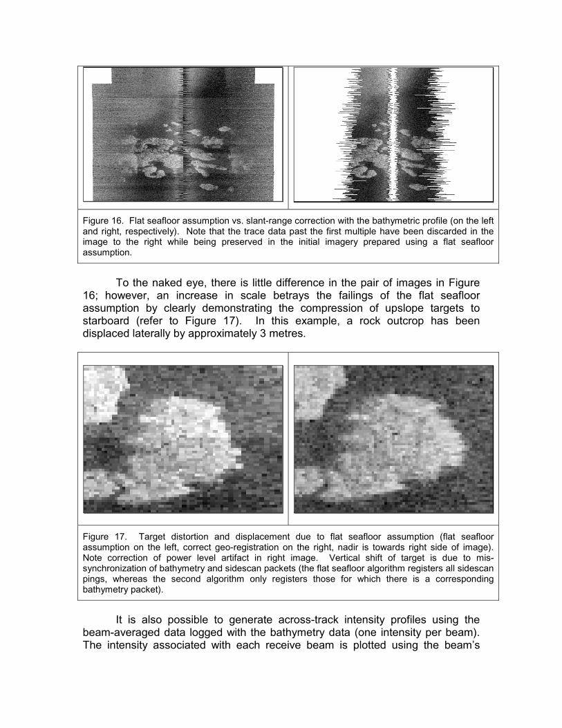
Images of the acoustic backscatter were prepared using both registrationtechniques and are shown in Figure 16. In this set of imagery, consecutive linesof data are simply stacked in time (time progressing down the page, port is to theright, starboard to the left) thus targets may suffer from along-track smearing andcompression due to yaw of vessel. The effect is similar in both images, thus isnegligible for the purposes of this illustration. Note that in the images createdusing the flat seafloor assumption that the data at nadir are noise due the nulls inthe dedicated port and starboard receive beams at nadir. The software used toperform the flat seafloor correction ignored this fact and incorrectly stitched in lowsignal-to-noise data from outside the beam pattern. In the properly registeredimages, the nadir area is left empty, respecting the nadir insensitivity inboard ofthe edge of both the port and starboard sidescan beams (which roll with thevessel).

Figure 16. Flat seafloor assumption vs. slant-range correction with the bathymetric profile (on the leftand right, respectively). Note that the trace data past the first multiple have been discarded in theimage to the right while being preserved in the initial imagery prepared using a flat seafloorassumption.

To the naked eye, there is little difference in the pair of images in Figure16; however, an increase in scale betrays the failings of the flat seafloorassumption by clearly demonstrating the compression of upslope targets tostarboard (refer to Figure 17). In this example, a rock outcrop has beendisplaced laterally by approximately 3 metres.

Figure 17. Target distortion and displacement due to flat seafloor assumption (flat seafloorassumption on the left, correct geo-registration on the right, nadir is towards right side of image).Note correction of power level artifact in right image. Vertical shift of target is due to mis-synchronization of bathymetry and sidescan packets (the flat seafloor algorithm registers all sidescanpings, whereas the second algorithm only registers those for which there is a correspondingbathymetry packet).

It is also possible to generate across-track intensity profiles using thebeam-averaged data logged with the bathymetry data (one intensity per beam).The intensity associated with each receive beam is plotted using the beam’s

across-track offset with the gaps in coverage between adjacent beams beingfilled by linear interpolation, effectively smearing the intensity values in theacross-track direction. The same subset of data was chosen to illustrate thepotential merits of using the beam-averaged intensities, as in Figure 18. There isno question that the trace data provide much better resolution (shown here at a0.5 metre resolution), however, it is plausible that the beam-averaged intensitiescould potentially be used to fill in the gaps at nadir in the trace dataset (resultsfrom early attempts at this technique are shown later in this paper). At the veryleast, the generation of backscatter imagery from the beam-averaged intensitiesprovides a check on the proper functioning of the slant-range correction algorithmas applied to the trace data.

Figure 18. Comparison of trace backscatter to beam-averaged intensities (on the left and right,respectively). In the imagery produced from the beam-averaged data, object boundaries aresmeared in the across-track direction. This results in an artificial enlargement of targets with objectboundaries being extended by half the beam footprint in the worst-case scenario. This problemcould potentially be overcome with an interpolation of higher-order between individual beamintensities.

Removal of Angular Response

A final radiometric reduction applied to the backscatter imagery is theremoval of the along-track banding due to the angular response of the seafloorand the residual beam pattern of the sonar transducer. This is done byproducing an average along-track angular response curve as a function ofincidence angle. After computing the curve, the mean of the curve is calculatedusing the off-nadir responses and is then used to reduce the absolute angularresponse to relative corrections that must be applied as a function of incidenceangle (e.g. suppress nadir by 3 dB as opposed to removing 60 dB, refer to Figure19). The mean along-track response was computed for a survey line that passedover a relatively featureless portion of the seafloor in the area and is shown inFigure 19 for both the trace and beam-averaged data. Slant-range correctedimagery were produced both with and without removal of the angular response,as in Figure 20.

Figure 19. Mean along-track angular response curves of trace and beam-averaged intensities.Note that there should exist a null at nadir in the trace data curve, however, this is not seen in thisplot due to the lack of roll stabilization and that the inboard edges of the port and starboardsidescan receive beams occasionally approach nadir.

Figure 20. Beam pattern filtering of trace data (raw data on left, filtered on right). Raw images areshown in the left hand column, while filtered images are shown in the right; images are shown ingreyscale and pseudo-colour to highlight the effect of the beam pattern removal.

Referring to Figure 20, it is evident that the majority of the angular responsehas been suppressed, however, a residual component remains in the inboardsections of the horizontal-range data. Complications are potentially due to thefollowing conflicting facts:

1. The dominant component of the along-track response is the angularresponse curve of the seafloor, thus the along-track response should becomputed relative to the seafloor normal, which varies with slope (for agiven incident angle, what is the average response).

2. The residual beam pattern of the sonar transducer will roll with the system(since the system was not roll stabilized), thus the along-track response

should be computed relative to the sonar transducer (for a given beam,what is the average response).

3. The angular response shape changes with sediment type, so deviationsfrom typical curves will remain in the data.

The angular response filtering improves the visual quality of the imagery to someextent though there remains further work to improve the performance of the filter.The same filtering can be done for the beam-averaged data with much betterresults, as shown in Figure 21.

Figure 21. Beam pattern filtering of beam-averaged data (raw data on left, filtered on right).Again, pseudo-colour was used to highlight the suppression of the angular response.

Map Production

Mosaics of the slant-range corrected data were generated using existingOMG software. Initial results, with and without angular response corrections, areshown in the Figures 22 and 23.

Figure 22. Mosaic of trace intensities (unfiltered image is on the left, angularresponse corrected image on the right). Pixel resolution is 2 metres.

As seen in Figure 22, all gain and power changes are corrected for, yielding avisually consistent image. The performance of the angular response filter is lesseffective than expected and further studies must be made into this (cf. section onFurther Research). Again, there exists no data below the vessel track due to thenulls in the sidescan receiver beam patterns.

Map sheets were created for the beam-averaged data as well and areshown in Figure 23. In this case, the angular response curve performed asexpected, removing most of the pattern except in cases of survey lines consistingmostly of featureless seafloor next to survey lines characterized by manytopographic features. This is due to the dissimilarity of the angular responsecurves between the two lines since both lines are reduced to different meanlevels. Thus the algorithm fails to bring the two datasets to a common level atthe equidistant seam that joins the coverage of both lines. This could easily be

improved by shortening the length of the averaging window when computing theangular response curves and allowing a single line of data to have multipleangular response curves.

Along with mosaics of trace and beam-averaged data, an attempt atcombining the two datasets was made in which the nadir gap of the trace datasetwas filled in with beam-averaged intensities. The different angular responsecurves for the trace data and beam-averaged intensities complicated the processof stitching the two data types together. This was overcome with slightmodifications to the slant-range correction algorithm, allowing for the suppression(or boosting) of one signal to match the other by recalculating the mean of theangular response curve and determining the additive constant required to matchthe means (this constant being added to the corrective offsets applied as afunction of incidence angle). Results of the blending of data types are shown inthe Figure 24, along with the original dataset (flat seafloor assumption, noradiometric corrections applied for power, gain or angular response).

Figure 25 emphasizes the effectiveness of the radiometric and geometriccorrections with two large-scale subsets from the maps of Figure 24. Even atthis scale, the low resolution of the beam-averaged data is of little consequenceand the beam-averaged data complements the trace intensities quite well. The

Figure 23. Mosaic of beam-averaged intensities (raw and beam pattern corrected).Pixel resolution is 2 metres.

different resolution of both data types becomes an issue at larger scales, such asin Figure 18. As mentioned earlier, the removal of the angular response issensitive to variations in topography and will perform poorly when neighbouringsurvey lines have vastly different angular response curves. This is particularlyevident in the upper right image of Figure 25, where several survey lines jointogether at the top of the image. Again, this can be improved by shortening thetime window over which the angular response curve is calculated.

FURTHER RESEARCH

Although resulting imagery is visually appealing, the maps cannot beanalysed numerically given that the measured intensities have only partially beenreduced to a measure of the true backscatter of the seafloor. Additionalcorrections remain:

1. The trace data must be normalized by pulse length to account for theensonified area. This involves using the bathymetry to compute thevarying grazing angles across-track.

Figure 24. Initial map prepared using a flat seafloor assumption, and final map. Thefinal map is a blend of trace intensities and beam-averaged intensities, and is fullycorrected for power and gain settings as well as mean along-track angular response.Pixel resolution is 2 metres.

2. The true source level must be determined and received intensitiesreferenced to this value such that backscatter values can be used in anabsolute manner.

3. The mean angular response curve of the trace data performs inadequatelyas a filter in the case of the trace data. An investigation must be madeinto the cause of the poor performance in hopes of developing a bettermethod of removing the average along-track angular response.

Figure 25. Large scale comparison of initial and final map products (left and right respectively).Radiometric artifacts due to power and gain have been completely compensated. The blendedsolution has the advantage of retaining the resolution of the trace data while incorporating the nadirbackscatter from the beam-averaged intensities.

The value of registering trace data past the beam coverage should beexamined, since the slant-range correction of the trace data currently ends at themultiple, i.e. 60 degrees off nadir. Although in this particular dataset the tracedata past the multiple are by and large noise, it may prove useful to be able toregister these data for applications when the sonar transducer is deployed on atow body allowing for data collection with lower incidence angles. Although thebathymetry coverage would be limited to the swath width, it may be possible togeographically register the data using the bathymetry provided by neighbouringlines of data or an underlying DTM built from the bathymetry data. At the veryleast, the remainder of the signal can be slant-range corrected using a flatseafloor assumption past the edge of the useful bathymetry (or a simple slopemodel provided by the bathymetry). The errors introduced by the flat seafloorassumption lessen with distance, thus this last solution may prove reasonable inaddition to being the simplest to implement.

While the focus of this work has been to extract useful backscatter datafrom SeaBat 8101 data with the single time-series trace data, it would be usefulto expand all of the software developed up to this point to be able to handle theinclusion of snippet data (made possible by recent RESON firmware upgrades).A test data set collected with a SeaBat 8111 has been provided by D. Lockhart ofThales GeoSolutions and will be used in future research.

SUMMARY

The RESON SeaBat 8101, as installed on the launches of the NOAA shipRainier, can log acoustic backscatter in two formats: a time-series of intensities(provided by the sidescan option), and beam-averaged intensities (associatedwith each bathymetric receive beam). Unfortunately, existing software tools onlyperform a flat seafloor assumption on the data provided via the sidescan option.Further to this, the raw backscatter data is uncorrected for variations in transmitpower and receiver gain.

Software tools have been developed to convert the Rainier SeaBat data(logged in XTF) into the OMG format. Once in the OMG format, it is possible toperform a proper slant-range correction by registering portions of the intensitytime-series using the bathymetric profile. Algorithms were developed to correctthe intensities for power and gain settings (as logged by the sonar). In addition,existing software in the OMG was updated to compute the average along-trackangular response of the trace and beam-averaged data. These radiometriccorrections can be applied during the slant-range correction process, resulting inhorizontal-range backscatter that is geometrically correct and radiometricallyconsistent across the dataset.

The software developed at this point is capable of producing mosaics ofacoustic backscatter both from the trace and beam-averaged data. A third optionwas investigated that allow for the blending of the two sources of data within asingle survey line. This was done to overcome the lack of data at nadir in the

trace dataset (due to a null at nadir in the sidescan receive beams, resulting in agap in any backscatter data directly below the vessel track). The blendedproduct preserves the high-resolution backscatter provided by the trace dataaway from nadir and fills in the gap at nadir with the beam-averaged data.

Further work will involve further reducing the backscatter data for pulsewidth and grazing angle, in addition to refining the removal of the angularresponse curve as it performs poorly for the trace data at this point. Finally, thelast radiometric correction is to reference all intensity values to a currentlyunknown source level such that they can be used in an absolute manner. Otherfuture research will focus on geo-registering the trace data past the end of thebathymetric coverage, in addition to adaptation of software to the inclusion ofsnippet data, as provided by recent firmware upgrades by RESON.

ACKNOWLEDGEMENTS

This research has been made possible through the funding of the U.S.Geological Survey. Thanks to Captain James Gardner (NOAA) foraccommodations onboard the Rainier during field trials and collection of the testdata set. Finally, special thanks to Burr Bridge (RESON, USA) and Jack Riley(NOAA) who both provided insight into the finer points of the RESON and XTFdata formats.

REFERENCES

Hughes Clarke, J.E., L.A. Mayer, and D.E. Wells (1996). “Shallow-WaterImaging Multibeam Sonars: A New Tool for Investigating Seafloor Processes inthe Coastal Zone and on the Continental Shelf.” Accepted for publication 7March 1996 in Marine Geophysical Researches.

Hughes Clarke, J.E. (1997). Field Laboratory using RESON SeaBat 9001and Seatex MRU-6. http://www.omg.unb.ca/~jhc/HYDRO_I_97/, February 2002.

Hughes Clarke, J.E. (1998). Multibeam Sonar Imaging. Lecture 10, 1998Coastal Multibeam Sonar Training Course. Dartmouth, Nova Scotia, 20-24 April,1998.

Lockhart, D., R. Pawlowski and E. Saade (2001). Multibeam BasedMapping of Fisheries Habitats in Alaska: Innovations in Imagery Products.http://www.ccom-jhc.unh.edu/shallow/abstracts/multibeam_fisheries.htm, Feb2002.

RESON (2000). SeaBat 8101 Multibeam Echosounder System.Operator’s Manual, v. 2.20, Goleta, California.