Geometric Applications of Principal Component Analysis · Zusammenfassung In vielen Anwendungen...

Geometric Applications

of Principal Component Analysis

Dissertation zur Erlangung des Doktorgrades

vorgelegt am

Fachbereich Mathematik und Informatik

der Freien Universitat Berlin

2008

von

Darko Dimitrov

Institut fur Informatik

Freie Universitat Berlin

Takustraße 9

14195 Berlin

[email protected]

Betreuer: PD Dr. Klaus Kriegel

Institut fur Informatik

Freie Universitat Berlin

Takustraße 9

D–14195 Berlin

Germany

[email protected]

Gutachter: PD Dr. Klaus Kriegel Prof. Dr. Gill Barequet

Institut fur Informatik Department of Computer Science

Freie Universitat Berlin Technion – Israel Institute of Technology

Takustraße 9 32000 Haifa

D–14195 Berlin Israel

Germany [email protected]

[email protected]

Termin der Disputation: 08. Dezember 2008

c© Darko Dimitrov, 2008.

Abstract

Bounding boxes are used in many applications for simplification of point sets or

complex shapes. For example, in computer graphics, bounding boxes are used to

maintain hierarchical data structures for fast rendering of a scene or for collision

detection. Additional applications include those in shape analysis and shape

simplification, or in statistics, for storing and performing range-search queries on

a large database of samples.

A frequently used heuristic for computing a bounding box of a set of points is

based on principal component analysis. The principal components of the point

set define the axes of the bounding box. Once the axis directions are given,

the dimension of the bounding box is easily found by the extreme values of the

projection of the points on the corresponding axis. Computing a PCA bounding

box of a discrete point set in Rd depends linearly on the number of points. The

popularity of this heuristic, besides its speed, lies in its easy implementation and

in the fact that usually PCA bounding boxes are tight-fitting.

In this thesis we investigate the quality of the PCA bounding boxes. We give

bounds on the worst case ratio of the volume of the PCA bounding box and the

volume of the minimum volume bounding box. We present examples of point

sets in the plane, where the worst case ratio tends to infinity. In these examples

some dense point clusters have a big influence on the directions of the principal

components, and the resulting PCA bounding boxes have much larger volumes

than the minimal ones. To avoid the influence of such non-uniform distributions

of the point sets, we consider PCA bounding boxes for continuous sets, especially

for the convex hulls of point sets, obtaining several variants of continuous PCA.

For those variants, we give lower bounds in arbitrary dimension, and upper

bounds in R2 and R

3. To obtain the lower bounds, we exploit a relation between

the perfect reflective symmetry and the principal components of point sets. Each

of the upper bounds in R2 and R

3 is obtained from two parameterized bounds.

The first bound is general for all bounding boxes, while to obtain the second

bound, we exploit some of the properties of PCA, combining them with ideas

from discrete geometry and integral calculus.

The relation between the perfect reflective symmetry and the principal com-

ponents of point sets, leads to a straightforward algorithm for computing the

planes of symmetry of perfect and approximate reflective symmetric point sets.

For the same purpose, we present an algorithm based on geometric hashing.

Zusammenfassung

In vielen Anwendungen werden große Punktmengen oder komplexe geometrische

Formen zur Vereinfachung durch sie umhullende Quader ersetzt (an Stelle dieses

selten gebrauchten deutschen Begriffs wird im Weiteren der englische Terminus

“Bounding Box” verwendet). Sie werden zum Beispiel in der Computergraphik

fur Datenstrukturen eingesetzt, die zum schnellen Rendering und zur Detektion

von Kollisionen dienen. Weitere Anwendungen findet man in der Analyse von

Formen oder in der Statistik zur Unterstutzung von Bereichsanfragen auf großen

Stichprobenmegen.

Eine sehr haufig verwendete Heuristik zur Berechnung einer Bounding Box

beruht auf der Hauptachsentransformation (oder Hauptkomponentenanalyse –

PCA). Wenn die Hauptachsen bekannt sind, kann man die entsprechend aus-

gerichtete Bounding Box leicht dadurch erhalten, dass die Minima und Maxima

der Projektionen der Punktmenge auf die einzelnen Achsen bestimmt werden.

Somit kann man die PCA–Bounding–Box einer Menge von n Punkten in Rd

in linearer Zeit berechnen. Neben diesem Laufzeitvorteil sind die unproblema-

tische Implementierung und die Erfahrung, dass die PCA–Bounding–Box in der

Regel ein sehr kleines Volumen hat, weitere Argumente, die fur den Einsatz der

Hauptachsentransformation sprechen.

In der vorliegenden Dissertation wird die Qualitat der PCA–Bounding–Box

hinsichtlich des Ziels der Volumenminimierung untersucht. Fur das Volumen-

verhaltnis zwischen PCA–Bounding–Box und der optimalen Bounding Box (mit

kleinstem Volumen) werden obere und untere Schranken nachgewiesen. Zuerst

werden Beispiele von Punktmengen in der Ebene konstruiert, die aufzeigen, dass

dieses Verhaltnis sich im schlechtesten Fall nicht begrenzen lasst, also gegen Un-

endlich geht. Bei der Konstruktion dieser Mengen spielen dichte Punktcluster

eine wichtige Rolle, welche die Hauptachsen in eine ungunstige Richtung zwin-

gen. Um den Einfluss solcher ungleichmaßiger Punktverteilungen zu vermeiden,

wird die Hauptachsentransformation auf stetige Punktmengen ausgedehnt, ins-

besondere auf die vollstandige konvexe Hulle einer Punktmenge oder auf den

Rand der konvexen Hulle. Fur diese PCA–Varianten wird wieder das Volumen-

verhaltnis zwischen PCA–Bounding–Box und der optimalen Bounding Box (im

schlechtesten Fall) untersucht. Es werden untere Schranken fur alle Dimensio-

nen gezeigt und auf der anderen Seite fur Punktmengen in R2 und R

3 obere

Schranken nachgewiesen. Zum Beweis der unteren Schranken wird ein Zusam-

viii ZUSAMMENFASSUNG

menhang zwischen der Spiegelsymmetrie einer Punktmenge und ihren Hauptach-

sen verwendet. Die oberen Schranken werden jeweils durch zwei parametrisierte

obere Schrankenfunktionen gewonnen. Dabei ist die erste Schrankenfunktion

allgemein fur jede Bounding Box gultig, wahrend die zweite die speziellen PCA–

Eigenschaften verwendet und diese mit Ideen und Hilfsmitteln aus Geometrie

und Integralrechnung kombiniert.

Der erwahnte Zusammenhang zwischen Spiegelsymmetrie und Hauptachsen

kann leicht in einen Algorithmus uberfuhrt werden, mit dem untersucht wer-

den kann, ob eine Punktmenge spiegelsymmetrisch oder naherungsweise spiegel-

symmetrisch ist. Fur diese Problemsstellung wird ein weiterer Algorithmus

vorgestellt, der auf geometrischem Hashing basiert.

Acknowledgments

First of all, I would like to thank my advisor Klaus Kriegel for his guidance, his

many good ideas and comments on our joint research, and his careful proofread-

ing of this thesis. In particular, I am very grateful to him for his extraordinarily

kind, helpful and immediate responses whenever they were needed.

I am grateful to Helmut Alt and Gunter Rote for giving me the opportunity

to be part of the department and get useful experience while working in it.

I would like to thank my colleagues from the work group Theoretical Com-

puter Science at the Free University Berlin for making it a creative and friendly

atmosphere to work in. Many thanks go to Gunter Rote and Christian Knauer for

sharing their knowledge and experience with me. While working on the thesis, I

have enjoyed and benefited from collaborating with several people and would like

to thank all of them: Tomas Dvorak, Petr Gregor, Mathias Holst, Elad Horev,

Christian Knauer, Roi Krakovski, Klaus Kriegel, Gunter Rote, Fabian Stehn,

Riste Skrekovski.

I am grateful to Gill Barequet for co-refereeing this thesis.

Finally, I want to express my gratitude to my family for their support during

my years of study and while working on this thesis. Most of all, I thank my sister

Tatjana for her unreserved and constant support.

Berlin, October 2008.

Contents

Abstract v

Zusammenfassung vii

1 Introduction 1

2 Preliminaries 7

2.1 Some Matrix Algebra Revision . . . . . . . . . . . . . . . . . . . . 7

2.2 Multivariate Analysis . . . . . . . . . . . . . . . . . . . . . . . . . 12

2.3 Principal Component Analysis . . . . . . . . . . . . . . . . . . . . 16

3 Lower Bounds on PCA Bounding Boxes 25

3.1 Approximation factors . . . . . . . . . . . . . . . . . . . . . . . . 25

3.2 Continuous PCA . . . . . . . . . . . . . . . . . . . . . . . . . . . 26

3.3 Lower Bounds . . . . . . . . . . . . . . . . . . . . . . . . . . . . . 27

4 Upper Bounds on PCA Bounding Boxes 35

4.1 Upper Bounds in R2 . . . . . . . . . . . . . . . . . . . . . . . . . 36

4.2 An upper bound in R3 . . . . . . . . . . . . . . . . . . . . . . . . 48

4.3 Open Problems . . . . . . . . . . . . . . . . . . . . . . . . . . . . 56

5 Closed-form Solutions for Continuous PCA 57

5.1 Evaluation of the Expressions for Continuous PCA . . . . . . . . 57

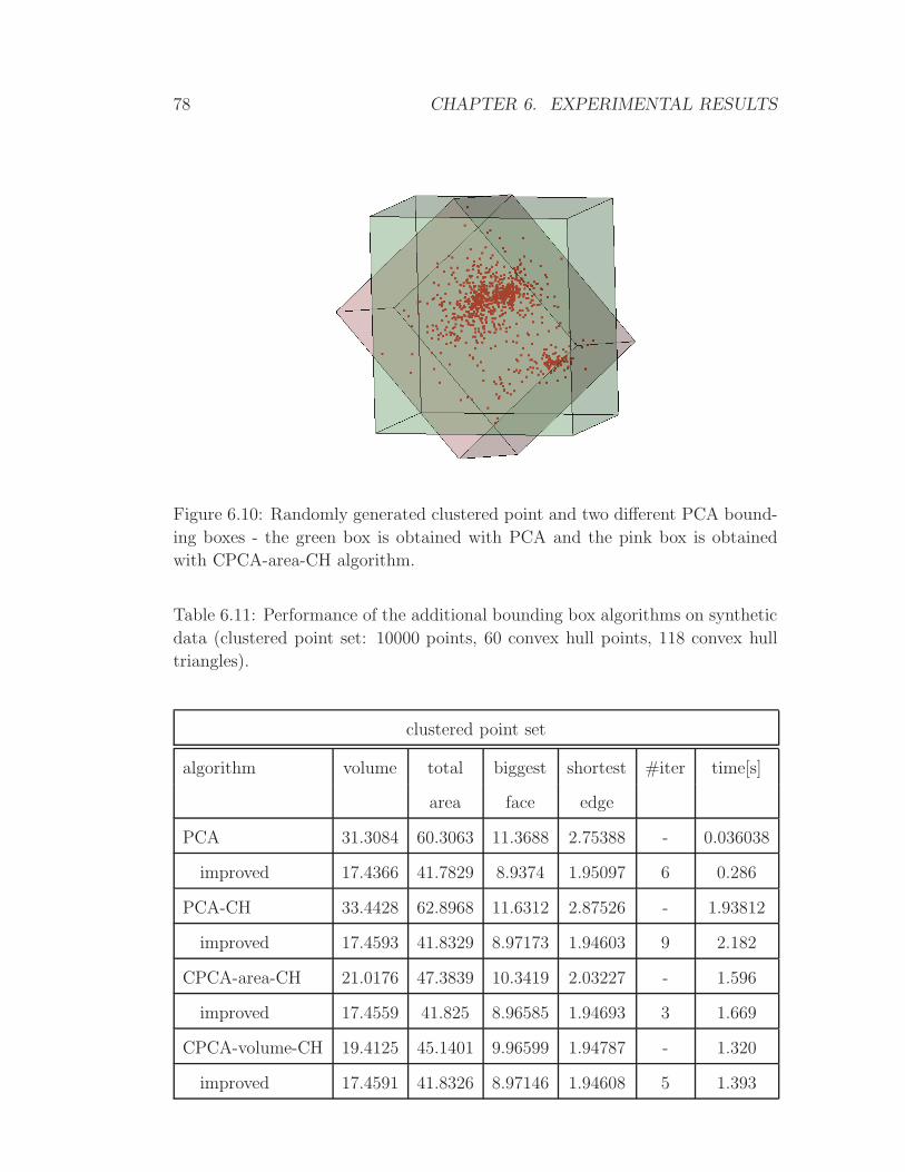
6 Experimental Results 63

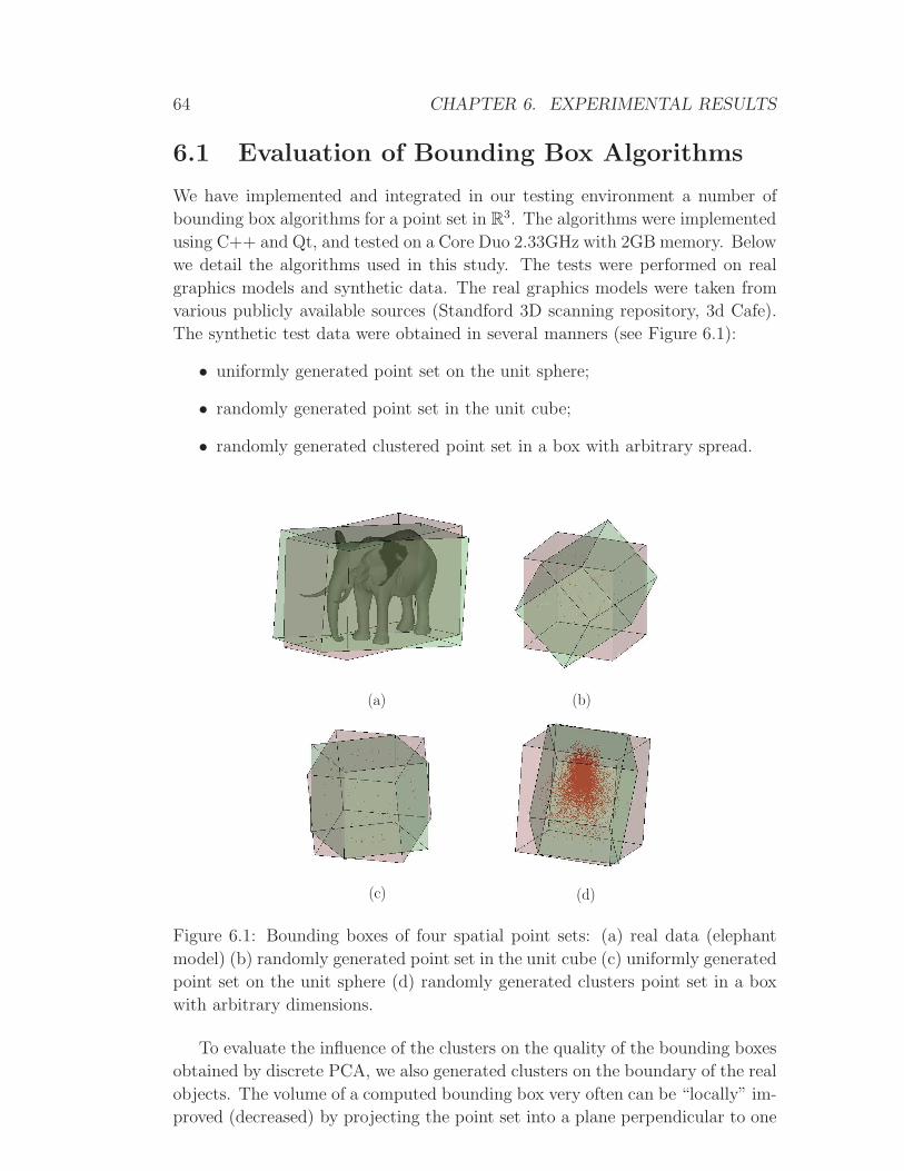
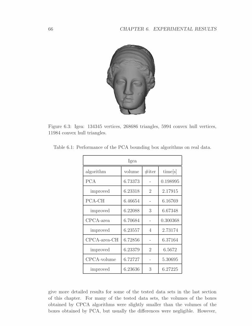
6.1 Evaluation of Bounding Box Algorithms . . . . . . . . . . . . . . 64

6.2 Conclusion . . . . . . . . . . . . . . . . . . . . . . . . . . . . . . . 71

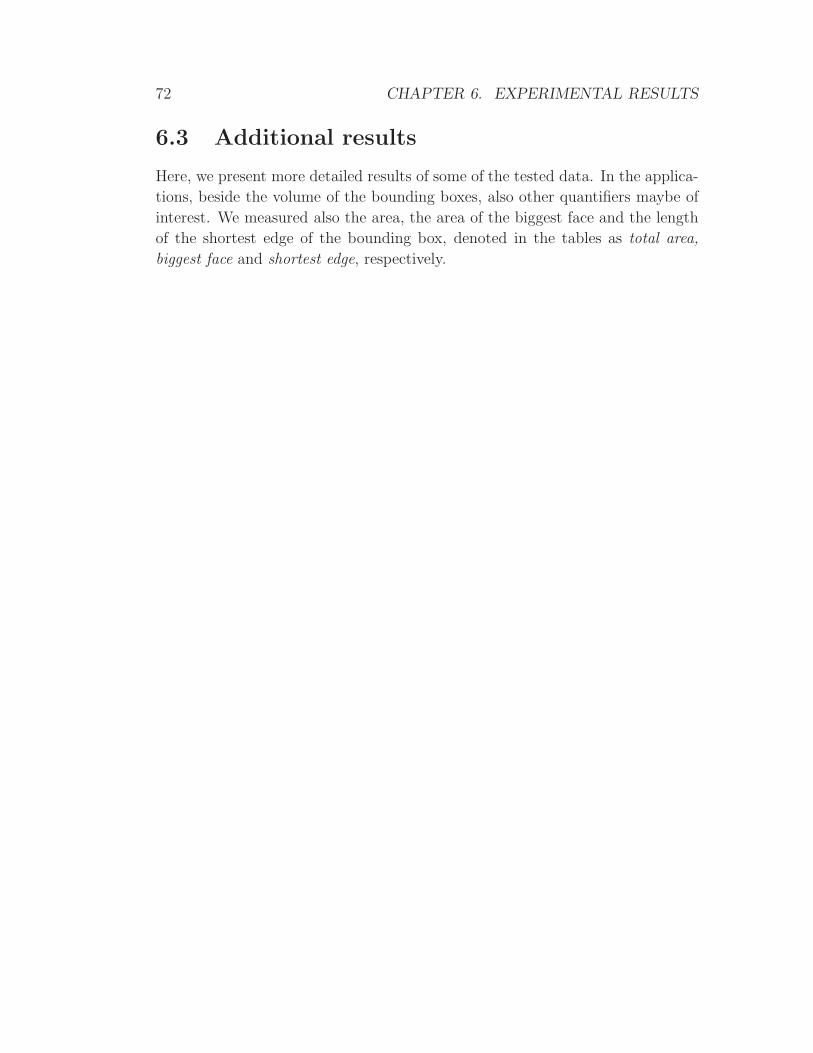
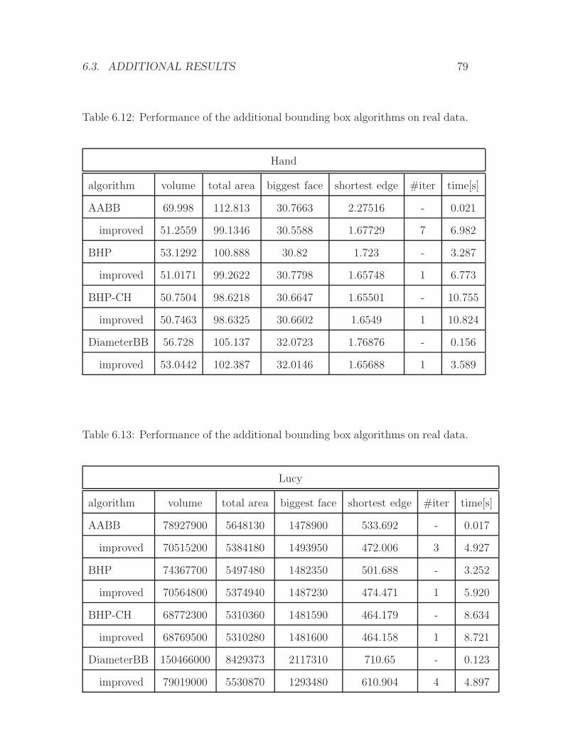
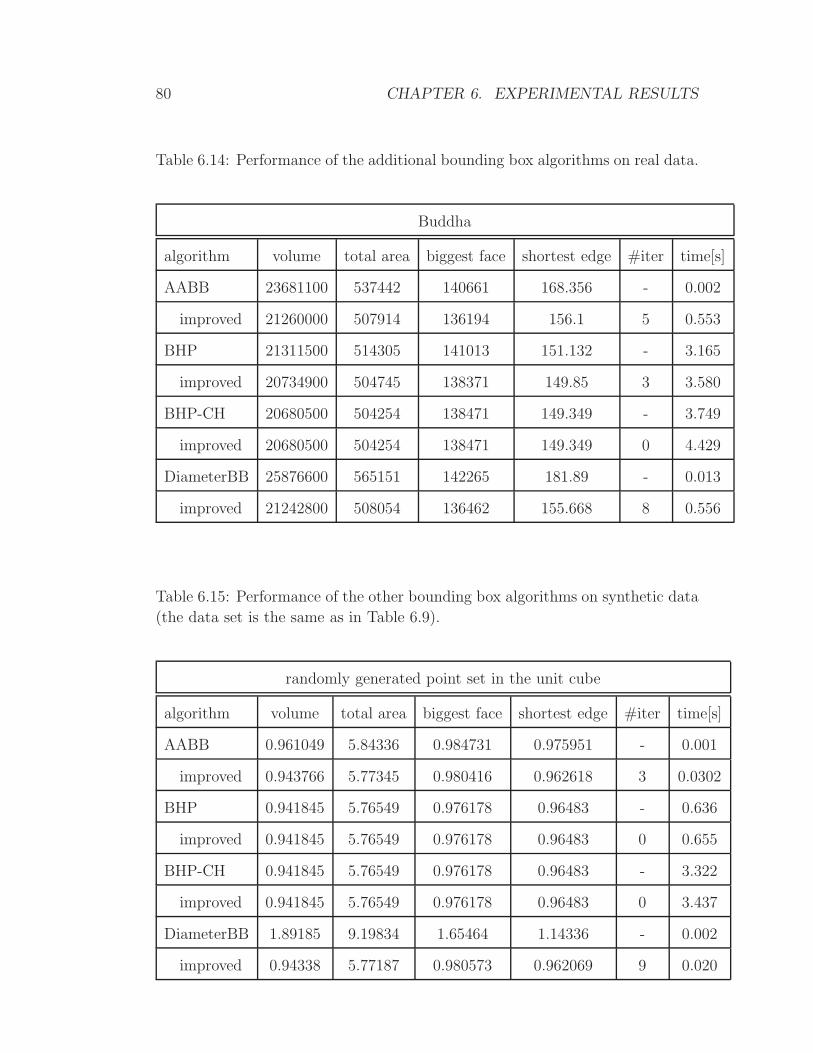
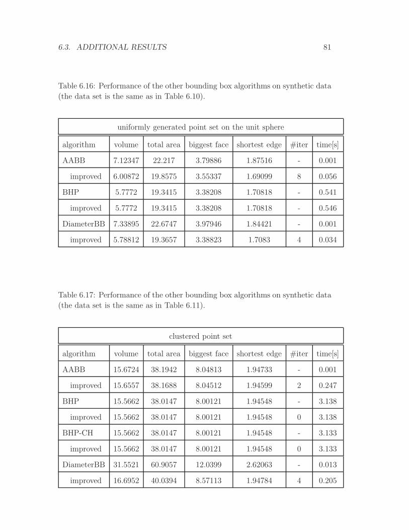
6.3 Additional results . . . . . . . . . . . . . . . . . . . . . . . . . . . 72

7 Reflective Symmetry - an Application of PCA 83

7.1 Introduction and Related Work . . . . . . . . . . . . . . . . . . . 83

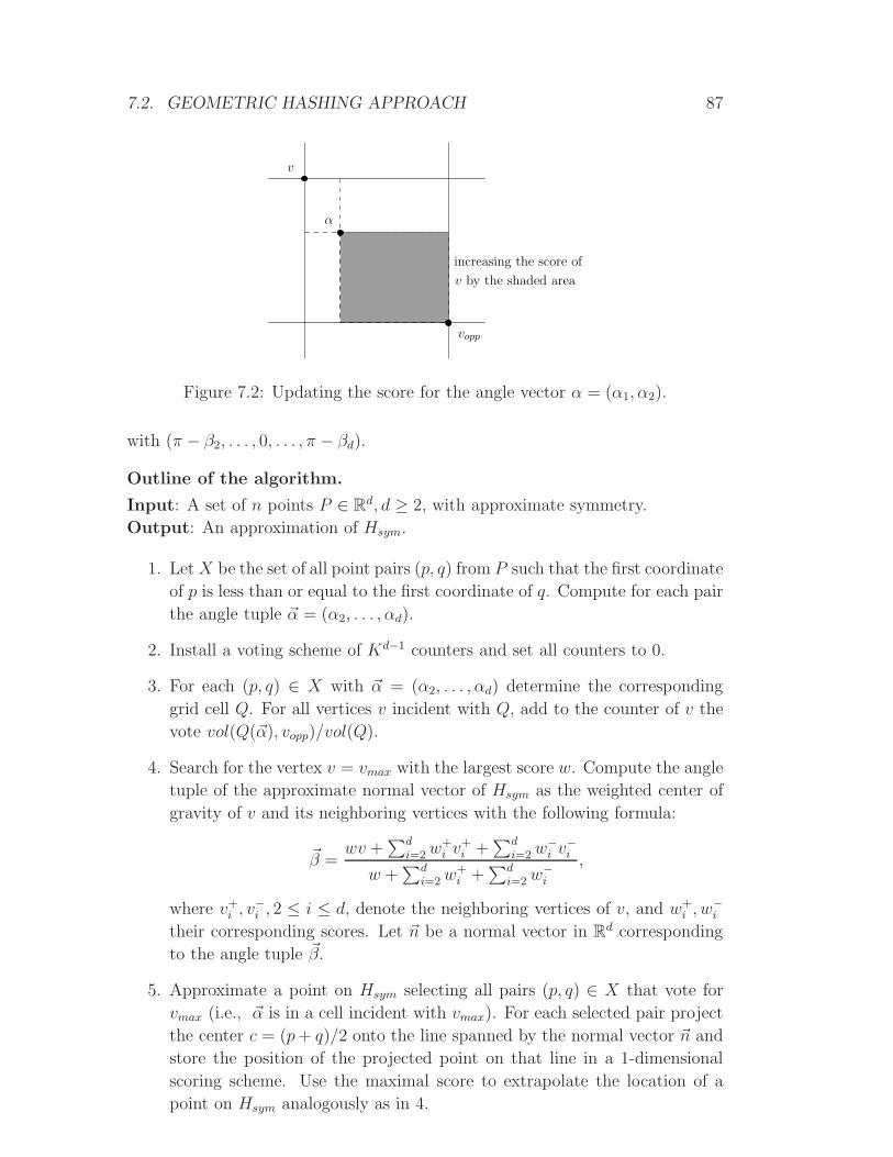
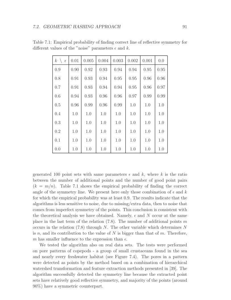
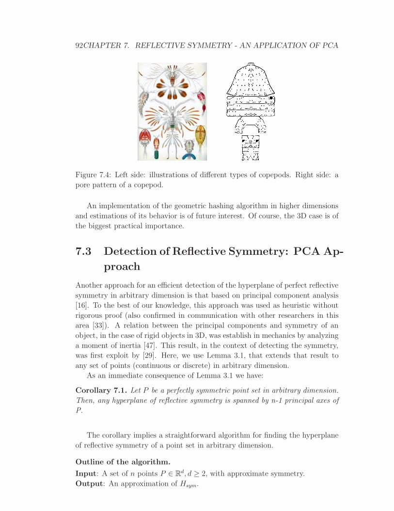
7.2 Geometric Hashing Approach . . . . . . . . . . . . . . . . . . . . 85

7.3 PCA Approach . . . . . . . . . . . . . . . . . . . . . . . . . . . . 92

Bibliography 95

xi

Chapter 1

Introduction

Principle component analysis (PCA), also known as Karhunen-Loeve transform,

or Hotelling transform, is one of the oldest and best known techniques of multi-

variate data analysis. The central idea of PCA is to reduce the dimensionality

of a data set represented by d interrelated variables, while retaining as much as

possible of the variation presented in the data set. This reduction is achieved

by representing the data set with respect to a new set of d variables (a new

coordinate system). The new set of variables, the so-called principle components

(PCs), are chosen such that they are uncorrelated, and they are ordered so that

the first few retain most of the variation present in all of the original variables.

For a graphical illustration of this reduction, we consider a simple example of

a 2-dimensional point set P in Figure 1.1 (in statistical data analysis PCA is

usually applied to higher dimensional point sets). Primarily, P is given with

X2

X1

PC2

PC1

(a) (b)

PP

Figure 1.1: (a) Plot of 80 observations on two variables X1 and X2. (b) Plot

of the same 80 observations from (a) with respect to their principal components

PC1 and PC2.

respect to two variables X1 and X2, where the origin is chosen at the center of

gravity of P . On the right side in Figure 1.1, we have the same point set with

respect to the coordinate system defined by the principal components PC1 and

1

2 CHAPTER 1. INTRODUCTION

PC2. As one can observe, the variable PC1 approximates the set of observa-

tions much better than any of the old variables X1 and X2 in the sense that the

orthogonal projection of P onto the line along PC1 has the maximal variance

among all possible projections. As it will be shown in the next chapter, if the

relationship between X1 and X2 (and therefore between PC1 and PC2) is linear,

than PC1 will contain the whole variance of the observations, and we can discard

PC2 without losing any information.

The reduction of the dimensionality of the data set has many applications in

various fields including computer vision, pattern recognition, visualization, data

analysis, etc.

The computation of the principle components reduces to the solution of

an eigenvalue-eigenvector problem for a positive-semidefinite symmetric matrix,

which can be solved efficiently.

Geometric applications of PCA

Most of the applications of PCA are non-geometric in their nature. However,

there are also a few purely geometric applications. A simple example is the

estimation of the undirected normals of the points. That heuristic is based on

the result by Pearson [38], who showed that the best-fitting line of the point

set in a d-dimensional space is determined by the first principal component of

the point set, and the direction of the last principal component is orthogonal

to the best-fitting hyperplane of the point set. Then, for a given point cloud

obtained from a smooth 2-manifold in R3 and a point p on the surface, we can

estimate the undirected normal to the surface at p as follows: find all the points

in a certain neighborhood of p and compute the principal components of those

points. The last principal component is an estimate of the undirected normal at

p. See Figure 1.2 for an illustration in R2.

p

npPC2

PC1

Figure 1.2: Estimation of the normal of the point p via principal components of

its neighboring points.

In this thesis, we concentrate on the geometric properties of the PCA con-

sidering two geometric applications of it. First, we consider the problem of

computing a bounding box of a point set in Rd, and second, we consider the

problem of detecting the perfect and approximate symmetry of a point set in Rd.

Substituting sets of points or complex geometric shapes with their bounding

3

boxes is motivated by many applications. For example, in computer graphics, it

is used to maintain hierarchical data structures for fast rendering of a scene or

for collision detection. Additional applications include those in shape analysis

and shape simplification, or in statistics, for storing and performing range-search

queries on a large database of samples.

Computing a minimum-area bounding rectangle of a set of n points in R2 can

be done in O(n log n) time, for example with the rotating calipers algorithm [49].

O’Rourke [35] presented a deterministic algorithm, a rotating calipers variant

in R3, for computing the minimum-volume bounding box of a set of n points

in R3. His algorithm requires O(n3) time and O(n) space. Barequet and Har-

Peled [5] have contributed two (1+ǫ)-approximation algorithms for the minimum-

volume bounding box of point sets in R3, both with nearly linear complexity.

The running times of their algorithms are O(n + 1/ǫ4.5) and O(n logn + n/ǫ3),

respectively.

Numerous heuristics have been proposed for computing a box which encloses

a given set of points. The simplest heuristic is naturally to compute the axis-

aligned bounding box of the point set. Two-dimensional variants of this heuristic

include the well-known R-tree, the packed R-tree [42], the R∗-tree [6], the R+-tree

[43], etc.

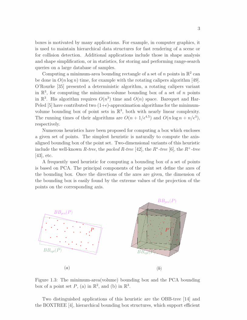
A frequently used heuristic for computing a bounding box of a set of points

is based on PCA. The principal components of the point set define the axes of

the bounding box. Once the directions of the axes are given, the dimension of

the bounding box is easily found by the extreme values of the projection of the

points on the corresponding axis.

P

BBpca(P )

BBopt(P )

(a) (b)

BBpca(P )

P

BBopt(P )

Figure 1.3: The minimum-area(volume) bounding box and the PCA bounding

box of a point set P , (a) in R2, and (b) in R

3.

Two distinguished applications of this heuristic are the OBB-tree [14] and

the BOXTREE [4], hierarchical bounding box structures, which support efficient


collision detection and ray tracing. Computing a bounding box of a set of points

in R2 and R

3 by PCA is simple and requires linear time. To avoid the influence of

the distribution of the point set on the directions of the PCs, a possible approach

is to consider the convex hull, or the boundary of the convex hull CH(P ) of the

point set P . Thus, the complexity of the algorithm increases to O(n log n). The

popularity of this heuristic, besides its speed, lies in its easy implementation and

in the fact that usually PCA bounding boxes are tight-fitting, see Chapter 6 and

[25] for some experimental results. Nevertheless, nothing was known about the

approximation quality of the PCA bounding box algorithm in the worst case.

Putting this problem into a striking phrase one could ask:

Is the computation of a bounding box by PCA only a heuristic (without any

guarantees), or is a bounding box computed by PCA a constant factor approxi-

mation of the minimum-volume bounding box?

In this thesis we give answers to that question for discrete point sets in arbi-

trary dimension and for continuous convex point sets in R2 and R

3.

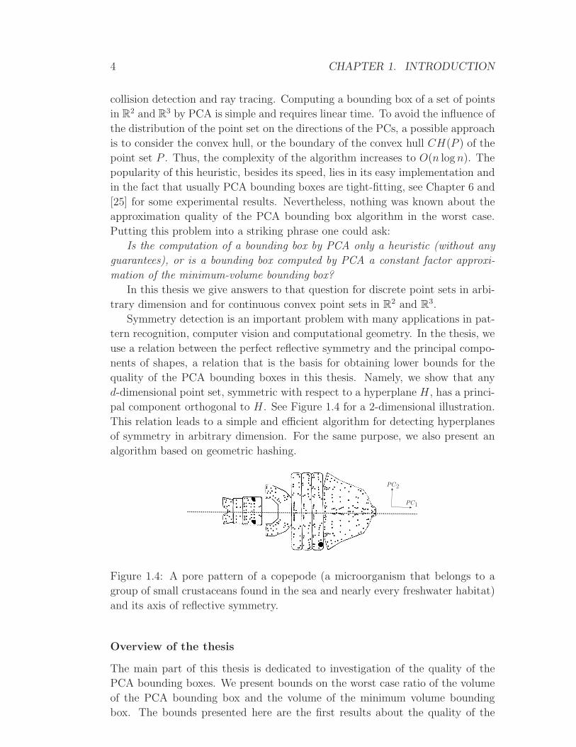
Symmetry detection is an important problem with many applications in pat-

tern recognition, computer vision and computational geometry. In the thesis, we

use a relation between the perfect reflective symmetry and the principal compo-

nents of shapes, a relation that is the basis for obtaining lower bounds for the

quality of the PCA bounding boxes in this thesis. Namely, we show that any

d-dimensional point set, symmetric with respect to a hyperplane H , has a princi-

pal component orthogonal to H . See Figure 1.4 for a 2-dimensional illustration.

This relation leads to a simple and efficient algorithm for detecting hyperplanes

of symmetry in arbitrary dimension. For the same purpose, we also present an

algorithm based on geometric hashing.

PC2

PC1

Figure 1.4: A pore pattern of a copepode (a microorganism that belongs to a

group of small crustaceans found in the sea and nearly every freshwater habitat)

and its axis of reflective symmetry.

Overview of the thesis

The main part of this thesis is dedicated to investigation of the quality of the

PCA bounding boxes. We present bounds on the worst case ratio of the volume

of the PCA bounding box and the volume of the minimum volume bounding

box. The bounds presented here are the first results about the quality of the

5

PCA bounding boxes. In addition, we consider the problem of detecting perfect

and approximate reflective symmetry of a point set, applying PCA and geometric

hashing approaches.

The structure and the contributions of the thesis are as follows.

• In Chapter 2 we discuss preliminaries that will be used in several of the

following chapters. We consider principal component analysis and present

some important results about it.

• In Chapter 3 we present lower bounds on the approximation factor of PCA

bounding boxes for point sets in arbitrary dimension. We present exam-

ples of discrete point sets in the plane, where the worst case ratio tends to

infinity. As a consequence, it follows that the discrete setting can not lead

to an approximation algorithm for the minimum-volume bounding box. To

avoid the influence of the distribution of the point set on the directions of

the principal components, we consider PCA bounding boxes for continuous

sets, especially for the convex hull of a point set, obtaining several vari-

ants of continuous PCA. We investigate the quality of the bounding boxes

obtained by the variants of continuous PCA related to the convex hull of

a point set, giving lower bounds on the approximation factor in arbitrary

dimension.

• In Chapter 4 we present upper bounds on the approximation factor of PCA

bounding boxes for continuous convex point sets in R2 and R

3.

• In Chapter 5 we consider the continuous version of PCA and give the

closed form solutions for the case when the point set is a polyhedron or a

polyhedral surface.

• In Chapter 6 we study the impact of the theoretical results on applications

of several PCA variants in practice. We analyze the advantages and disad-

vantages of the different variants on realistic inputs, randomly generated

inputs, and specially constructed (worst case) instances. Also, we evaluate

and compare the performances of several existing bounding box algorithms

we have implemented.

• In Chapter 7 we exploit a relation between the principal components and

a hyperplane of symmetry of a perfect reflective-symmetric point set in

arbitrary dimension. This relation implies a straightforward algorithm for

detecting hyperplanes of symmetry. In addition, for the same purpose,

we present an algorithm based on geometric hashing. 2D versions of both

algorithms have been implemented and tested on real and synthetic data.

The generation of the synthetic data is based on a probabilistic model,

which additionally is used for a probabilistic analysis of the reliability of

the geometric hashing algorithm.


Most of the results presented in this thesis have been published in [10], [11],

[12], and [13].

Chapter 2

Preliminaries

In this chapter we collect known concepts and results which will be used sev-

eral times within this thesis. The central part of this chapter is Section 2.3,

where we consider principal component analysis and present some important

results about it. To keep the presentation self-contained, in Section 2.1 and Sec-

tion 2.2, we give an overview of some definitions and results from linear algebra

and multivariate analysis. For those results which are normally not treated in

undergraduate mathematics courses, we give additional comments and proofs.

The results presented in this chapter are adapted from [8, 16, 34, 45].

2.1 Some Matrix Algebra Revision

Multivariate data consist of observations on several different variables for a num-

ber of individuals or objects. We denote the number of variables by d, and the

number of individuals or objects by n. Thus in total we have n×d measurements.

Let arj be the r-th observation of the j-th variable. The matrix whose element

in the r-th row and j-th column is arj, is called the data matrix and is denoted

by A. Thus

A =

a11 a12 . . . a1d

a21 a22 . . . a2d

......

. . ....

an1 an2 . . . and

.

If A has n rows and d columns we say it is of order n × d. The transpose of a

matrix A is formed by interchanging the rows and columns, and we denote it by

AT . A matrix with column-order one is called a column vector. Thus

a =

a1

a2

...

an

7

8 CHAPTER 2. PRELIMINARIES

is a column vector with n components. The data matrix can be seen as n row

vectors, which we denote by aT1 to aT

n , or as d column vectors, which we denote

by b1 to bd. Thus

A =

aT1

aT2...

aTn

= (b1,b2, . . . ,bd)

where aTi denotes the transpose of ai. Note that the vectors are printed in bold

type, and the matrices in ordinary type.

Also note that row vectors are points in a d-dimensional space, while the

column vector are points in an n-dimensional space. When comparing variables,

we compare column vectors.

A matrix is squared if the number of its rows equals to the number of its

columns. A squared matrix is said to be diagonal if all its off-diagonal elements

are zero. The identity matrix, denoted by I, is a diagonal matrix whose diagonal

elements are all unity. The trace of a squared matrix A of order d× d is the sum

of the diagonal terms, namely∑d

i=1 aii, and will be denoted by tr(A).

A determinant of a squared matrix A is defined as

det(A) =∑

sgn(τ) a1τ(1) . . . adτ(d),

where the summation is taken over all permutations τ of (1, 2, . . . , d), and sgn(τ)

denotes the signature of the permutation τ : +1 or −1, depending on whether τ

can be written as the product of an even or odd number of transpositions.

A squared matrix A is non-singular if det(A) 6= 0; otherwise it is singular.

The inverse matrix of matrix A is the unique matrix A−1 satisfying

AA−1 = A−1A = I.

The inverse exists if and only if A is non-singular, that is, if and only if det(A) 6=0.

A set of vectors x1, . . . ,xd is said to be linearly dependent if there exist

constants c1, . . . , cd which are not all zero, such that

d∑

i=1

cixi = 0.

Otherwise the vectors are said to be linearly independent. This definition leads

on the idea of a rank of a matrix, which is defined as the maximum number of

rows which are linearly independent (or equivalently as the maximum number

of columns which are linearly independent). In other words, the rank is the

dimension of the subspace spanned by vectors consisting of all the rows (or all

2.1. SOME MATRIX ALGEBRA REVISION 9

the columns). We denote by rank(A) the rank of matrix A. The following

relations hold:

rank(A) = rank(AT )

= rank(AAT )

= rank(AT A) (2.1)

and

rank(A) = rank(BA) = rank(AC), (2.2)

for all non-singular matrices B, C of appropriate order.

Orthogonality. Two vectors x, y of order d × 1 are said to be orthogonal if

xT y = 0.

They are said to be orthonormal if they are orthogonal and

xT x = yTy = 1.

A squared matrix B is said to be orthogonal if

BT B = BBT = I

so that the rows (columns) of B are orthonormal. It is clear that B must be

non-singular with

B−1 = BT .

A transformation from a d × 1 vector x to an n × 1 vector y given by

y = Ax + b, (2.3)

where A is an n × d matrix and b is an n × 1 vector, is called a linear transfor-

mation. For n = d the transformation is called non-singular if A is non-singular,

and in that case the inverse transformation is

x = A−1(y − b).

An orthogonal transformation is defined by

y = Ax, (2.4)

where A is an orthogonal matrix. Geometrically, an orthogonal matrix represents

a linear transformation which consists of a rigid rotation, plus maybe reflection,

since it preserves distances and angles. The determinant of an orthogonal matrix

is ±1. If the determinant is +1, the corresponding transformation is a pure rota-

tion, while if the determinant is −1, the corresponding transformation involves

in addition a reflection.


Quadratic forms and definiteness. A quadratic form in d variables, x1, . . . , xd is

a function consisting of all possible second-order terms, namely

a11x21 + · · ·+ addx

2d + a12x1x2 + · · · + ad−1,dxd−1xd =

∑

1≤i,j≤d

aijxixj .

This can be conveniently written as xT Ax, where xT = [x1, . . . , xd]. The matrix

A is usually taken to be symmetric. A squared matrix A and its associated

quadratic form is called:

• positive definite if xT Ax > 0 for every x 6= 0;

• positive semidefinite if xT Ax ≥ 0 for every x.

Positive definite quadratics forms have matrices of full rank and can be repre-

sented as

A = QQT (2.5)

where Q is non-singular. Then y = QTx transforms the quadratic form xT Ax

to the reduced form y21 + · · ·+ y2

d which only involves squared terms.

If A is a positive semidefinite of rank m(< d), then A can also be expressed

in the form of Equation (2.5), but with a matrix Q of order d × m which is of

rank m. This is sometimes called the Young-Householder factorization of A.

Eigenvalues and eigenvectors. If Σ is a quadratic matrix of order d × d, then

q(λ) = det(Σ − λI) (2.6)

is a d-th order polynomial in λ. It is called the characteristic polynomial of

Σ. The d roots of q(λ), λ1, λ2, . . . , λd, possibly complex numbers, are called

eigenvalues of Σ. Some of the λi will be equal if q(λ) has multiple roots. To each

eigenvalue λi, there corresponds a vector ci, called an eigenvector, such that

Σci = λici. (2.7)

The eigenvectors are not unique as they contain an arbitrary scale factor, and

thus, they are usually normalized so that cTi ci = 1. When there are equal

eigenvalues, the corresponding eigenvectors can, and will, be chosen to be or-

thonormal.

If x and y are eigenvectors for λi and α ∈ R, then x + y and αx are also

eigenvectors for λi. Thus, the set of all eigenvectors for λi forms a subspace

which is called the eigenspace of Σ for λi. The maximal number of independent

eigenvectors of the eigenspace determines the dimension of the eigenspace.

Some useful properties are as follows:.

(a)d∑

i=1

λi = tr(Σ); (2.8)

2.1. SOME MATRIX ALGEBRA REVISION 11

(b)d∏

i=1

λi = det(Σ); (2.9)

(c) If Σ is real symmetric matrix, then its eigenvalues and eigenvectors are

real;

(d) If, further, Σ is positive definite, then all the eigenvalues are strictly posi-

tive;

(e) If Σ is positive semidefinite of rank m (< d), then Σ has m positive and

(d − m) zero eigenvalues;

(f) For two different eigenvalues, the corresponding normalized eigenvector are

orthonormal;

(g) If we form a d×d matrix C, whose i-th column is the normalized eigenvector

ci, then CT C = I and

CT Σ C = Λ (2.10)

where Λ is a diagonal matrix whose diagonal elements are λ1, . . . , λd. This

is called the canonical reduction of Σ.

The matrix C is a quadratic form of Σ to the reduced form which only involves

squared terms. Writing x = Cy we have

xT Σx = yT CTΣCy

= yT Λy

= λ1y21 + · · ·+ λmy2

m (2.11)

where m=rank (Σ).

From Equation (2.10) we may also write

Σ = CΛCT = λ1c1cT1 + · · ·+ λmcmcT

m. (2.12)

This is called the spectral decomposition of Σ.

Differentiation with respect to vectors. Suppose we have a differentiable function

of d variables, say f(x1, . . . , xd). The notation ∂f/∂x will be used to denote a

column vector whose i-th component is the partial derivation ∂f/∂xi.

Suppose that the function is the quadratic form xT Σx, where Σ is a d × d

symmetric matrix. Then it is straightforward to show that

∂f

∂x= 2Σx. (2.13)


2.2 Multivariate Analysis

2.2.1 Means, variances, covariances, and correlations

Let X be a random vector consisting of d random variables. Random vectors

will be printed with capital letters in bold type. In this section we will present

quantities that summarize a probability distribution of X. In the univariate

case, it is often done by giving the first two moments, namely the mean and

the variance (or its square root, the standard deviation). To summarize multi-

variate distributions, we need to find the mean and variance of the d variables,

together with a measure of the way each pair of variables is related. The latter

target is achieved by calculating a set of quantities called covariances, or their

standardized counterparts called correlations.

Means. The mean vector µT = [µ1, . . . µd] such that

µi = E(Xi) =∑

xPi(x) (2.14)

is the mean of the i-th component of X. Here Pi(x) denotes the (marginal)

probability distribution of Xi. This definition is given for the case where Xi is

discrete. If Xi is continuous, then

E(Xi) =

∫ ∞

−∞xfi(x)dx, (2.15)

where fi(x) is the probability density function of Xi.

Variances. The variance of the i-th component of X is given by

var(Xi) = E[(Xi − µi)2]

= E(X2i ) − µ2

i . (2.16)

This is usually denoted by σ2i in the univariate case, but in order to tie in with

the covariance notation given below, we denote it by σii in the multivariate case.

Covariances. The covariance of two variables Xi and Xj is defined by

cov(Xi, Xj) = E[(Xi − µi)(Xj − µj)]. (2.17)

Thus, it is the product moment of the two variables about their respective means.

In particular, if i = j, we note that the covariance of a variable with itself

is simply the variance of the variable. The covariance of Xi ad Xj is usually

denoted by σij . Thus, for i = j, σii denotes the variance of Xi. Equation 2.17 is

often written in the equivalent alternative form

σij = E[XiXj] − µiµj. (2.18)

2.2. MULTIVARIATE ANALYSIS 13

The covariance matrix. Given d variables, there are d variances and d(d − 1)/2

covariances, and all these quantities are second moments. It is often useful to

present these quantities in a symmetric d×d matrix, denoted by Σ, whose (i, j)-th

element is σij . Thus,

Σ =

σ11 σ12 . . . σ1d

σ21 σ22 . . . σ2d

......

. . ....

σd1 σd2 . . . σdd

. (2.19)

The matrix is variously called the dispersion matrix, the variance-covariance

matrix, or simply the covariance matrix, and we will use the latter term. The

diagonal terms of Σ are the variances, while the off-diagonal terms are the co-

variances.

Using Equations (2.17) and (2.18), we can express Σ in two alternative useful

forms, namely

Σ = E[(X − µ)(X − µ)T ]

= E[XXT ] − µµT . (2.20)

Linear combination. Perhaps the main use of covariances is as a stepping stone to

the calculations of correlations (see below), but they are also useful for a variety

of other purposes. Later in Section 2.3, we will consider the variance of a linear

combination of the components of X. Consider the general linear combination

Y = aT X

where aT = [a1, . . . , ad] is a vector of constants. Then Y is a univariate random

variable. Its mean is clearly given by

E(Y ) = aTµ (2.21)

while its variance is given by

var(Y ) = E[{aT (X − µ)}2]. (2.22)

As aT (X − µ) is a scalar and therefore equal to its transpose, we can express

var(Y ) in terms of Σ, using Equation (2.20), as

var(Y ) = E[aT (X − µ)(X − µ)Ta]

= aT E[(X − µ)(X − µ)T]a

= aT Σa. (2.23)


Correlations. Although covariances are useful for many mathematical purposes,

they are rarely used as descriptive statistics. If two variables are related in a

linear way, then the covariance will be positive or negative depending on whether

the relationship has a positive or negative slope. But the size of the coefficient is

difficult to interpret because it depends on the units in which the two variables

are measured. Thus the covariance is often standardized by dividing by the

product of the standard deviations of the two variables to give a quantity called

the correlation coefficient. The correlation between variables Xi and Xj will be

denoted by ρij , and is given by

ρij = σij/σiσj (2.24)

where σi and σj denote the standard deviations of Xi and Xj. It can be shown

that ρij is always a value between −1 and +1.

The correlation coefficient provides a measure of the linear association be-

tween two variables. The coefficient is positive if the relationship between the

two variables has a positive slope so that the ‘high’ values of one variable tend to

go with ‘high’ values of the other variable. Conversely, the coefficient is negative

if the relationship has a negative slope.

If two variables are independent then their covariance, and their correlation,

are zero. But it is important to note that the converse of this statement is not

true. Here is an example: Suppose that the random variable X is uniformly

distributed on the interval from −1 to 1, and Y = X2. Then, Y is completely

determined by X, so that X and Y are dependent, but their correlation is zero.

This emphasizes the fact that the correlation coefficient may be misleading if the

relationship between two variables is non-linear. However, if the two variables

follow a bivariate normal distribution, then it turns out that zero correlation

does imply independence. A detailed explanation and further results about the

relation between the correlation and independence of the random variables can

be found, for example, in [45].

The correlation matrix. From the definition of the correlation, it follows that for

given d variables, there are d(d−1)/2 distinct correlations. A d×d matrix, whose

(i, j)-th element is defined to be ρij is called the correlation matrix and will be

denoted by P (capital Greek letter rho). A correlation matrix is symmetric with

the diagonal terms all equal unity.

In order to relate the covariance matrix and correlation matrix, let us define

a d× d diagonal matrix D, whose diagonal terms are the standard deviations of

the components of X, so that

2.2. MULTIVARIATE ANALYSIS 15

D =

σ1 0 . . . 0

0 σ2 . . . 0...

.... . .

...

0 0 . . . σd

. (2.25)

Then the covariance matrix and correlation matrices are related by

Σ = DPD

or

P = D−1ΣD−1 (2.26)

where the diagonal terms of the matrix D−1 are the reciprocals of the respective

standard deviations.

The rank of Σ and P. We complete this section with a discussion of the matrix

properties of Σ and P, and in particular of their rank.

Firstly, we show that both Σ and P are positive semidefinite. As any variance

must be non-negative, we have that

var(aTX) ≥ 0 for every a.

But var(aT X) = aT Σa, and so Σ must be semidefinite. We also note that Σ is

related to P by Equation (2.26), where D is non-singular, and so it follows that

P is also positive semidefinite.

Because D is non-singular, we may also use Equations (2.26) and (2.2) to

show that the rank of P is the same as the rank of Σ. This rank must be less

than or equal d.

If Σ (and hence P) has rank d, then Σ (P) is positive definite, as in this case,

var(aT X) is strictly greater than zero for every a 6= 0. But if rank(Σ) < d, then

Σ (P) is singular, and this indicates a linear constraint on the components of X.

This means that there exists a vector a 6= 0 such that var(aT X) = aT Σa is zero,

indicating that Σ is positive semidefinite rather than positive definite.

When rank(Σ) < d, the components of X are sometimes said to be ‘linearly

dependent’, using this term in its algebraic sense. However, statisticians often

use this term to mean a linear relationship between the expected values of the

random variables. It needs to be emphasized that a constraint of the latter type

will generally not produce a singular Σ. If two variables are correlated, it does

not mean that one of them is redundant, although if the correlation is very high

then one of them may be ‘nearly redundant’ and the covariance matrix will be

‘nearly singular’.


2.3 Principal Component Analysis

2.3.1 Motivation

The central idea and motivation of principal component analysis (abbreviated

to PCA) is to reduce the dimensionality of a point set by identifying the most

significant directions (principal components). Let P = {p1,p2, . . . ,pn} be a set

of vectors (points) in Rd, and µ = (µ1, µ2, . . . , µd) ∈ R

d be the center of gravity

of P . For 1 ≤ k ≤ d, we use pik to denote the k-th coordinate of the vector pi.

Given two vectors u and v, we use 〈u,v〉 to denote their inner product. For any

unit vector v ∈ Rd, the variance of P in direction v is

var(P,v) =1

n

n∑

i=1

〈pi − µ , v〉2. (2.27)

The most significant direction corresponds to the unit vector v1 such that var(P,v1)

is maximum. In general, after identifying the j most significant directions

v1, . . . ,vj, the (j +1)-st most significant direction corresponds to the unit vector

vj+1 such that var(P,vj+1) is maximum among all unit vectors perpendicular to

v1,v2, . . . ,vj.

From the multivariate analysis point of view, we can consider P as a sam-

ple of points that represents a d-dimensional vector of random variables XT

=[X1, X2, . . .Xd]. Namely, to each coordinate of the points corresponds one ran-

dom variable. As it will be shown in the next subsection principal components

are uncorrelated linear combinations of the original variables of X, and are de-

rived in decreasing order of importance so that, for example, the first principal

component accounts for as much possible of the variation in the original data.

The transformation is in fact an orthogonal rotation in d-space. The technique of

finding this transformation is called principal component analysis. PCA origi-

nated in the work by Karl Pearson [38] around the turn of the 20th century, and

was further developed in the 1930s by Harold Hotelling [20] using the approach

described in the next subsection.

The usual objective of the analysis is to study if the first few components

account for most of the variation in the original data. If they do, then it is argued

that the effective dimensionality of the problem is less than d. In order words, if

some of the original variables are highly correlated, they are effectively ‘saying

the same thing’ and there may be near-linear constraints on the variables. In

this case it is hoped that the first few components will be intuitively meaningful,

will help us understand the data better, and will be useful in subsequent analysis

where we can operate with a smaller number of variables. The reduction of the

complexity (dimensionality), we have illustrated in the introduction (Figure 1.1)

on an unrealistic, but simple, case where d = 2.

We note that PCA is a statistical technique which does not require the user

to specify an underlying statistical model to explain the ‘error’ structure. In par-

2.3. PRINCIPAL COMPONENT ANALYSIS 17

ticular, no assumption is made about the probability distribution of the original

variables, though more meaning can generally be given to the components in the

case where the observations are assumed to be multivariate normal [16].

2.3.2 Derivation of principal components

Suppose that X is a d-dimensional random vector with mean µ and covariance

matrix Σ. Our problem is to find a new set of variables, say Y1, Y2, . . . , Yd which

are uncorrelated and whose variances decrease from first to last. Each Yj is taken

to be a linear combination of the X’s, so that

Yj = a1jX1 + a2jX2 + · · ·+ apjXd

= aTj X (2.28)

where aTj = [a1j , a2j , . . . , apj] is a vector of constants. Equation (2.28) con-

tains an arbitrary scale factor. We therefore impose the condition that aTj aj =∑d

k=1 a2kj = 1. We will call such a linear transformation a standardized linear

transformation. We shall see that this particular normalization procedure ensures

that the overall transformation is orthogonal - in other words, that distances in

d-space are preserved.

The first principal component, Y1, is found by choosing a1 so that Y1 has

the largest possible variance. In other words, we choose a1 so as to maximize

the variance of aT1 X subject to the constraint that aT

1 a1 = 1. This approach,

originally suggested by Harold Hotelling [20], gives equivalent results to that of

Karl Pearson [38], which finds the hyperplane in d-space such that the total sum

of squared perpendicular distances from the point to the hyperplane is minimized.

The second principal component is found by choosing a2 so that Y2 has the

largest possible variance for all combinations of the form of Equation (2.28) which

are uncorrelated with Y1. Similarly, we derive Y3, . . . , Yd, so as to be uncorrelated

and to have decreasing variance.

We begin by finding the first component. We want to choose a1 so as to

maximize the variance of Y1 subject to normalization constraint that aT1 a1 = 1.

Now

var(Y1) = var(aT1 X)

= aT1 Σa1 (2.29)

using Equation (2.23). Thus we take aT1 Σa1 as our objective function.

The standard procedure for maximizing a function of several variables subject

to one or more constraints is the method of Lagrange multipliers. With just one

constraint, this method uses the fact that the stationary points of a differentiable


function of d variables, say f(x1, . . . , xd), subject to a constraint g(x1, . . . xd) = c,

are such that there exists a number λ, called the Lagrange multiplier, such that

∂f

∂xi

− λ∂g

∂xi

= 0 i = 1, . . . , d (2.30)

at the stationary points. These d equations, together with the constraints, are

sufficient to determine the coordinates of the stationary points and the corre-

sponding value of λ. Further investigations are needed to see if a stationary

point is a maximum, minimum or saddle point. It is helpful to form a new

function L(x), such that

L(x) = f(x) − λ[g(x) − c]

where the term in the square brackets is of course zero. Then the set of equations

in (2.30) may be written simply as

∂L

∂x= 0

using the definition given in Section 2.1. Applying this method to our problem,

we write

L(a1) = aT1 Σa1 − λ(aT

1 a1 − 1).

Then, using Equation 2.13, we have

∂L

∂a1

= 2Σa1 − 2λa1.

Setting this equal to 0, we have

(Σ − λI)a1 = 0, (2.31)

where I is the identity matrix of order d × d. We now come to the crucial step

in the argument. If Equation (2.31) is to have a solution for a1, other than the

null vector, then (Σ− λI) must be a singular matrix. Thus λ must be chosen so

that

det(Σ − λI) = 0.

Thus a non-zero solution for Equation (2.31) exists if and only if λ is an eigenvalue

of Σ. But Σ will generally have d eigenvalues, which must all be nonnegative as

Σ is positive semidefinite. Let λ1 ≥ λ2 ≥ · · · ≥ λd ≥ 0 be the eigenvalues of Σ.

In the case where some of the eigenvalues are equal, there is no unique way of

choosing the corresponding eigenvectors. Then, the eigenvectors associated with

multiple roots will be chosen to be orthogonal.

Which eigenvalue shall we choose to determine the first principal component?

Now,


var(aT1 X) = aT

1 Σa1

= aT1 λa1 using Equation (2.31)

= λ.

As we want to maximize this variance, we choose λ to be the largest eigenvalue,

namely λ1. Then, using Equation (2.31), the principal component, a1, which

we are looking for must be the eigenvector of Σ corresponding to the largest

eigenvalue.

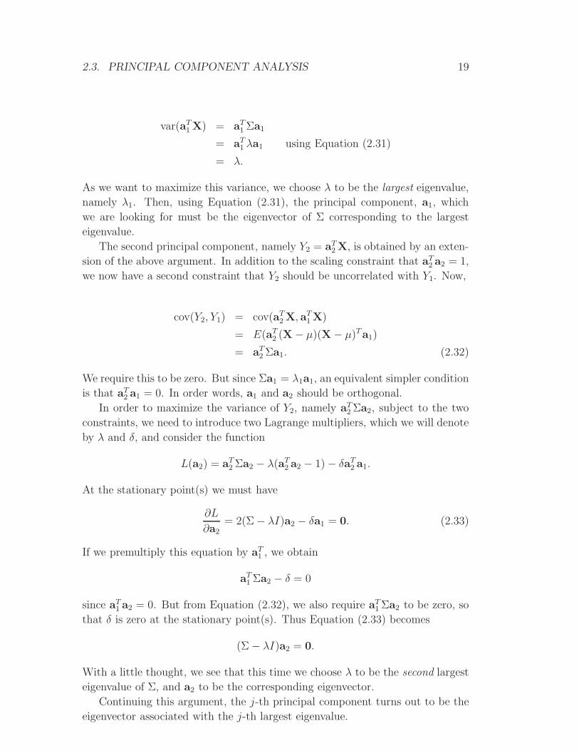
The second principal component, namely Y2 = aT2 X, is obtained by an exten-

sion of the above argument. In addition to the scaling constraint that aT2 a2 = 1,

we now have a second constraint that Y2 should be uncorrelated with Y1. Now,

cov(Y2, Y1) = cov(aT2 X, aT

1 X)

= E(aT2 (X − µ)(X − µ)Ta1)

= aT2 Σa1. (2.32)

We require this to be zero. But since Σa1 = λ1a1, an equivalent simpler condition

is that aT2 a1 = 0. In order words, a1 and a2 should be orthogonal.

In order to maximize the variance of Y2, namely aT2 Σa2, subject to the two

constraints, we need to introduce two Lagrange multipliers, which we will denote

by λ and δ, and consider the function

L(a2) = aT2 Σa2 − λ(aT

2 a2 − 1) − δaT2 a1.

At the stationary point(s) we must have

∂L

∂a2= 2(Σ − λI)a2 − δa1 = 0. (2.33)

If we premultiply this equation by aT1 , we obtain

aT1 Σa2 − δ = 0

since aT1 a2 = 0. But from Equation (2.32), we also require aT

1 Σa2 to be zero, so

that δ is zero at the stationary point(s). Thus Equation (2.33) becomes

(Σ − λI)a2 = 0.

With a little thought, we see that this time we choose λ to be the second largest

eigenvalue of Σ, and a2 to be the corresponding eigenvector.

Continuing this argument, the j-th principal component turns out to be the

eigenvector associated with the j-th largest eigenvalue.


2.3.3 Definition and some properties of the principal com-

ponents

Now, we give the definition of the principal component transformation of a ran-

dom vector X for a general dimension d.

Definition 2.1. If X is a random vector with mean µ and covariance Σ, then

the principal component transformation is the transformation

X → Y = CT (X− µ), (2.34)

where C is orthogonal, CT ΣC = Λ is a diagonal matrix, with diagonal elements

λ1 ≥ λ2 ≥ · · · ≥ λd ≥ 0. The strict positivity of the eigenvalues λi, is guaranteed

if Σ is positive definite. This representation of Σ follows from its spectral decom-

position (Equation (2.10)). The i-th principal component of X may be defined

as the i-th element of the vector Y, namely as

Yi = ci(X − µ). (2.35)

Here ci is the i-th column of C and may be called the i-th vector of principal

component loadings. The function Yd may be called the last principal component

of X.

In the sequel, we summarize some fundamental properties of principal com-

ponents, which are immediately observed from the derivation and definition of

principal components.

Proposition 2.1. If X is a random vector with mean µ and covariance Σ, and

Y is as defined in (2.34), then

(a) E(Yi) = 0;

(b) var(Yi) = λi;

(c) cov(Yi, Yj) = 0, i 6= j;

(d) var(Y1) ≥ var(Y2) · · · ≥ var(Yd) ≥ 0;

(e)∑d

i=1 var(Yi) = tr(Σ);

(f)∏d

i=1 var(Yi) = det(Σ)

Proof. (a)-(d) follow from Definition 2.1 and the properties of the expectation

operator. (e) follows from (b) and the fact that tr(Σ) is the sum of the eigenvalues

(Equation (2.8)). (f) follows from (b) and the fact that det(Σ) is the product of

the eigenvalues (Equation (2.9)).

From the derivation of the principal components in the previous section fol-

lows the next important property.


Proposition 2.2. No standardized linear combination of X has a variance larger

than λ1, the variance of the first principal component.

Similarly, as in Proposition 2.2, it follows that the last principal component

of X has a variance which is smaller than that of any other standardized linear

combination. The intermediate components have a maximal variance property

given by the following proposition.

Proposition 2.3. If α = aTX is a standardized linear combination of X which

is uncorrelated with the first k principal components of X, then the variance of

α is maximized when α is the (k + 1)-st principal component of X.

Now, we give a geometric property of principal components. Let A be a

positive definite matrix of order d × d . Then

(x − α)T A−1(x − α) = c2 (2.36)

represents an ellipsoid in d dimensions with center x = α. On shifting the center

to x = 0, the equation becomes

xT A−1x = c2. (2.37)

Definition 2.2. Let x be a point on the ellipsoid defined by (2.36) and let

f(x) = ‖x − α‖ denote the squared distance between x and α. A line through α

and x for which x is a stationary point of f(x) is called a principal axis of the

ellipsoid. The distance ‖x − α‖ is called the length of the principal semi-axis.

Proposition 2.4. Let λ1, . . . , λd be the eigenvalues of A satisfying λ1 > λ2 >

· · · > λd. Suppose that c1, . . . , cd are the corresponding eigenvectors. For the

ellipsoids (2.36) and (2.37), we have

(a) The direction of the i-th principal axis coincides with ci.

(b) The length of the i-th principal semi-axis is cλ1/2i .

Proof. It is sufficient to prove the result for (2.37). The problem reduces to

finding the stationary points of f(x) = xTx subject to x lying on the ellip-

soid xT A−1x = c2. From (2.13), we have that the derivation of xT A−1x is

2xTA−1. Thus a point y represents a direction tangent to the ellipsoid at x if

2yTA−1x = 0.

The derivative of f(x) is 2x so the directional derivative of f(x) in the direc-

tion y is 2yTx = 0; that is if

yT A−1x = 0 ⇒ yTx = 0.

This condition is satisfied if and only if A−1x is proportional to x; that is if and

only if x is an eigenvector of A−1.

Setting x = βci in (2.37) gives β2/λ = c2, so β = cλ1/2i . Thus, the theorem

is proved.


x1

x2

y1 = c1Tx

y2 = c2Tx

a

b

Figure 2.1: Ellipsoid xT A−1x = 1. Lines defined by y1 and y2 are the first and

second principal axes, ‖a‖ = λ11/2, ‖b‖ = λ2

1/2.

If we rotate the coordinate axes with the transformation y = CTx, where C

is obtained by the spectral decomposition of A (A = CΛC), we find that (2.37)

reduces to ∑y2

i /λi = c2.

Figure 2.1 gives a pictorial representation.

With A = I, Equation (2.37) reduces to a hypersphere with λ1 = · · · = λd = 1

so that the λs are not distinct and the above theorem fails; that is, the positions

of ci, i = 1, . . . d through the sphere are not unique and any rotation will suffice.

In general, if λi = λi+1, the section of the ellipsoid is circular in the plane

generated by ci and ci+1. Although we can construct two perpendicular axes for

the common root, their position through the circle is not unique.

An immediate consequence of Proposition 2.4 follows.

Corollary 2.1. Consider the family of d-dimensional ellipsoids

XT Σ−1X = c2. (2.38)

where X is a random vector with covariance matrix Σ. The principal components

of X define the principal axes of these ellipsoids.

The properties of PCA, mentioned till now, were obtained from a known pop-

ulation covariance matrix Σ. In practice the covariance matrix Σ (or correlation

matrix P) is rarely known and hence the eigenvalues λ1, . . . , λd and its corre-

sponding eigenvectors must be estimated from the random sample (sample data

matrix). However, in that case one can similarly obtain the results presented

in this chapter. We conclude this chapter with the following property that is

geometrically equivalent to the algebraic properties from Propositions 2.2 and

2.3.


Proposition 2.5. Let p1, . . . ,pn be observations in a d-dimensional space. A

measure of ‘goodness-of-fit’ of a q-dimensional hyperplane to p1, . . . ,pn can be

defined as the sum of squared perpendicular distances of p1, . . . ,pn from the

hyperplane. This measure is minimized when the q-dimensional hyperplane is

spanned by the first q principal components of p1, . . . ,pn.

This property can be viewed as an alternative derivation of the principal

components. Rather than adapting the algebraic definition of population prin-

cipal components, given above in this section, there is an alternative geometric

definition of sample principal components. They are defined as the linear func-

tions (projections) of p1, . . . ,pn that successively define hyperplanes of dimen-

sion 1, 2, . . . , q, . . . , (d− 1) for which the sum of squared perpendicular distances

of p1, . . . ,pn from the hyperplane is minimized. This definition provides another

way in which principal components can be interpreted as accounting for as much

as possible of the total variation in the data, within lower-dimensional space.

In fact, this is essentially the approach adopted by Pearson [38], although he

concentrated on the two cases, where q = 1 and q = d− 1. Given a set of points

in d-dimensional space, Pearson found the ‘best-fitting line’ and ‘best-fitting hy-

perplane’ in the sense of minimizing the sum of squared deviations of the points

from the line or hyperplane. The best-fitting line determines the first principal

component, although Pearson did not use this terminology, and the direction of

the last principal component is orthogonal to the best-fitting hyperplane.

Chapter 3

Lower Bounds on the Quality of

the PCA Bounding Boxes

In this and the next chapter we study the quality of the PCA bounding boxes,

obtaining bounds on the worst case ratio of the volume of the PCA bounding box

and the volume of the minimum-volume bounding box. We present examples of

point sets in the plane, where the worst case ratio tends to infinity. To avoid

the influence of the distribution of the point set on the directions of the PCs,

we consider PCA bounding boxes for continuous sets, especially for the convex

hull of a point set, obtaining several variants of continuous PCA. In this chapter,

we investigate the quality of the bounding boxes obtained by the variants of

continuous PCA related to the convex hull of a point set, giving lower bounds

on the approximation factor in an arbitrary dimension.

3.1 Approximation factors

Given a point set P ⊆ Rd we denote by BBpca(P ) the PCA bounding box of

P and by BBopt(P ) the bounding box of P with smallest possible volume. The

ratio of the two volumes κd(P ) = Vol(BBpca(P ))/Vol(BBopt(P )) defines the

approximation factor for P , and

κd = sup{κd(P ) | P ⊆ R

d, Vol(CH(P )) > 0}

defines the general PCA approximation factor.

Since bounding boxes of a point set P (with respect to any orthogonal coordi-

nate system) depend only on the convex hull of CH(P ), the construction of the

covariance matrix should be based only on CH(P ) and not on the distribution

of the points inside. Using the vertices, i.e., the 0-dimensional faces of CH(P )

to define the covariance matrix Σ we obtain a bounding box BBpca(d,0)(P ). We

denote by κd,0(P ) the approximation factor for the given point set P and by

κd,0 = sup{κd,0(P ) | P ⊆ R

d, Vol(CH(P )) > 0}

25

26 CHAPTER 3. LOWER BOUNDS ON PCA BOUNDING BOXES

1stPC

1stPC

2ndPC

2ndPC

(b)(a)

Figure 3.1: Four points and their PCA bounding-box (left). A dense collection

of additional points significantly affect the orientation of the PCA bounding-box

(right).

the approximation factor in general. The example in Figure 3.1 shows that

κ2,0(P ) can be arbitrarily large if the convex hull is a thin, slightly “bulged

rectangle”, with a lot of additional vertices in the middle of the two long sides.

Since this construction can be lifted into higher dimensions we obtain a first

general lower bound.

Proposition 3.1. κd,0 = ∞ for any d ≥ 2.

To overcome this problem, one can apply a continuous version of PCA taking

into account (the dense set of) all points on the boundary of CH(P ), or even

all points in CH(P ). In this approach X is a continuous set of d-dimensional

vectors and the coefficients of the covariance matrix are defined by integrals

instead of finite sums. If CH(P ) is known, the computation of the coefficients

of the covariance matrix in the continuous case can also be done in linear time,

thus, the overall complexity remains the same as in the discrete case. Note that

for for d = 1 the above problem is trivial, because the PCA bounding box is

always optimal, i.e., κ1,0 is 1.

3.2 Continuous PCA

Variants of the continuous PCA applied to triangulated surfaces of 3D objects

were presented by Gottschalk et. al. [14], Lahanas et. al. [25] and Vranic et. al.

[50]. In what follows, we briefly review the basics of the continuous PCA in a

general setting.

Let X be a continuous set of d-dimensional vectors with constant density.

Then, the center of gravity of X is

c =

∫x∈X

xdx∫x∈X

dx. (3.1)

3.3. LOWER BOUNDS 27

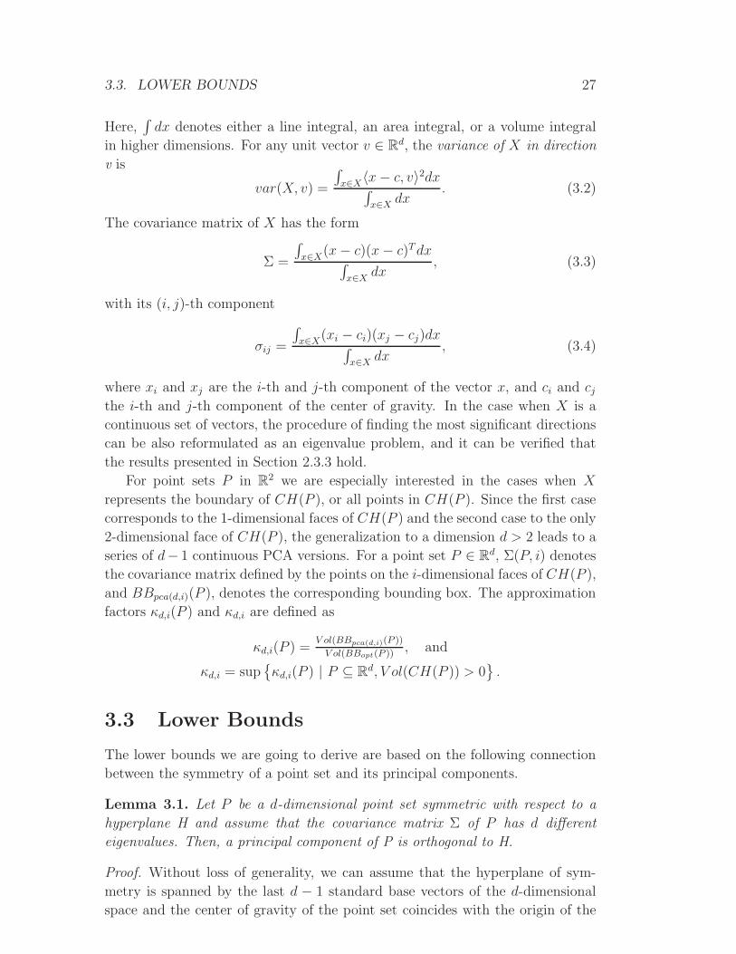
Here,∫

dx denotes either a line integral, an area integral, or a volume integral

in higher dimensions. For any unit vector v ∈ Rd, the variance of X in direction

v is

var(X, v) =

∫x∈X

〈x − c, v〉2dx∫x∈X

dx. (3.2)

The covariance matrix of X has the form

Σ =

∫x∈X

(x − c)(x − c)T dx∫x∈X

dx, (3.3)

with its (i, j)-th component

σij =

∫x∈X

(xi − ci)(xj − cj)dx∫x∈X

dx, (3.4)

where xi and xj are the i-th and j-th component of the vector x, and ci and cj

the i-th and j-th component of the center of gravity. In the case when X is a

continuous set of vectors, the procedure of finding the most significant directions

can be also reformulated as an eigenvalue problem, and it can be verified that

the results presented in Section 2.3.3 hold.

For point sets P in R2 we are especially interested in the cases when X

represents the boundary of CH(P ), or all points in CH(P ). Since the first case

corresponds to the 1-dimensional faces of CH(P ) and the second case to the only

2-dimensional face of CH(P ), the generalization to a dimension d > 2 leads to a

series of d− 1 continuous PCA versions. For a point set P ∈ Rd, Σ(P, i) denotes

the covariance matrix defined by the points on the i-dimensional faces of CH(P ),

and BBpca(d,i)(P ), denotes the corresponding bounding box. The approximation

factors κd,i(P ) and κd,i are defined as

κd,i(P ) =V ol(BBpca(d,i)(P ))

V ol(BBopt(P )), and

κd,i = sup{κd,i(P ) | P ⊆ R

d, V ol(CH(P )) > 0}

.

3.3 Lower Bounds

The lower bounds we are going to derive are based on the following connection

between the symmetry of a point set and its principal components.

Lemma 3.1. Let P be a d-dimensional point set symmetric with respect to a

hyperplane H and assume that the covariance matrix Σ of P has d different

eigenvalues. Then, a principal component of P is orthogonal to H.

Proof. Without loss of generality, we can assume that the hyperplane of sym-

metry is spanned by the last d − 1 standard base vectors of the d-dimensional

space and the center of gravity of the point set coincides with the origin of the


d-dimensional space, i.e., c = (0, 0, . . . , 0). Thus, we can write P = P+ ∪ P−,

where each point p− from P− has a counterpoint p+ in P+ (and vice versa) such

that p− and p+ differ only in the first coordinate, namely p−1 = −p+1 . Then, we

can rewrite (3.4) as

σij =

∫p∈P

(pi − ci)(pj − cj)dp∫

p∈Pdp

=

∫p∈P+ pipjdp∫

p∈P+ dp+

∫p∈P−

pipjdp∫

p∈P−dp

,

and

σ1j =

∫p∈P+ p1pjdp∫

p∈P+ dp+

∫p∈P−

p1pjdp∫

p∈P−dp

=

∫p∈P+ p1pjdp∫

p∈P+ dp+

∫p∈P+ −p1pjdp∫

p∈P+ dp.

Then, the components σ1j , for 2 ≤ j ≤ d, are 0. Due to symmetry the

components σj1 are also 0. Thus, the covariance matrix has the form

Σ =

σ11 0 . . . 0

0 σ22 . . . σ2d

......

. . ....

0 σd2 . . . σdd

. (3.5)

We note that the same argument carry thorough in the case when P is a discrete

point set.

The characteristic polynomial of Σ is

det(Σ − λ I) = (σ11 − λ)f(λ), (3.6)

where f(λ) is a polynomial of degree d − 1, with coefficients determined by the

elements of the (d − 1) × (d − 1) submatrix of Σ. From this it follows that σ11

is a solution of the characteristic equation, i.e., it is an eigenvalue of Σ and the

vector (1, 0, ...,0) is its corresponding eigenvector (principal component), which

is orthogonal to the assumed hyperplane of symmetry.

We start with a generalization of Proposition 3.1.

Proposition 3.2. κd,i = ∞ for any d ≥ 4 and any 1 ≤ i < d − 1.

Proof. We use a lifting argument to show that for any point set P ⊆ Rk there

is a point set P ′ ⊆ Rk+1 such that κk,i(P ) ≤ κk+1,i+1(P

′), and consequently

κk,i ≤ κk+1,i+1.

Let Σ be the covariance matrix of P with eigenvalues λ1 > λ2 > · · · > λk,

and corresponding eigenvectors v1, v2, . . . vk. We define the point set P ′(h) =

P × [−h, h], h ∈ R+. Let Σ′(h) be the covariance matrix of P ′(h). Obviously,

the point set P ′(h) is symmetric with respect to the hyperplane H = Rk × {0},

and by Lemma 3.1, the vector vk+1 = (0, . . . , 0, 1) is an eigenvector of Σ′(h).

Let λ(h) be the corresponding eigenvalue of vk+1. Since λ(h) = var(P ′, vk+1)


is a quadratic function of h, with limh→0 λ(h) = 0, we can choose a value h0

such that λ(h0) is smaller than the other eigenvalues of Σ′. Let v be an ar-

bitrary direction in Rk. Then, by definition of P ′, the variance of P ′ in the

direction (v, 0) remains the same as the variance of P in the direction v. Thus,

we can conclude that the eigenvalues of Σ′ are λ1 > λ2 > · · · > λk > λ(h0),

with corresponding eigenvectors (v1, 0), (v2, 0), . . . (vk, 0), vk+1, and consequently

Vol(BBpca(k+1,i+1)(P′)) = 2 h0 Vol(BBpca(k,i)(P )).

On the other hand, the bounding box BBh0 = BBopt(P )× [−h0, h0] is also a

bounding box of P ′. Therefore, we obtain

κk+1,i+1 ≥ κk+1,i+1(P′) =

Vol(BBpca(k+1,i+1)(P′))

Vol(BBopt(P′))

≥ Vol(BBpca(k+1,i+1)(P′))

Vol(BBh0)

≥ 2h0Vol(BBpca(k,i)(P ))2h0Vol(BBopt(P ))

≥ κk,i.

Now, we can establish κd,i ≥ κd−1,i−1 ≥ . . . ≥ κd−i,0 = ∞.

This way, there remain only two interesting cases for a given d: the factor

κd,d−1 corresponding to the boundary of the convex hull, and the factor κd,d

corresponding to the full convex hull.

3.3.1 Lower bounds in R2

The result obtained in this subsection can be seen as a special case of the result

obtained in Subsection 3.3.3. To gain a better understanding of the problem and

the obtained results, we consider it separately.

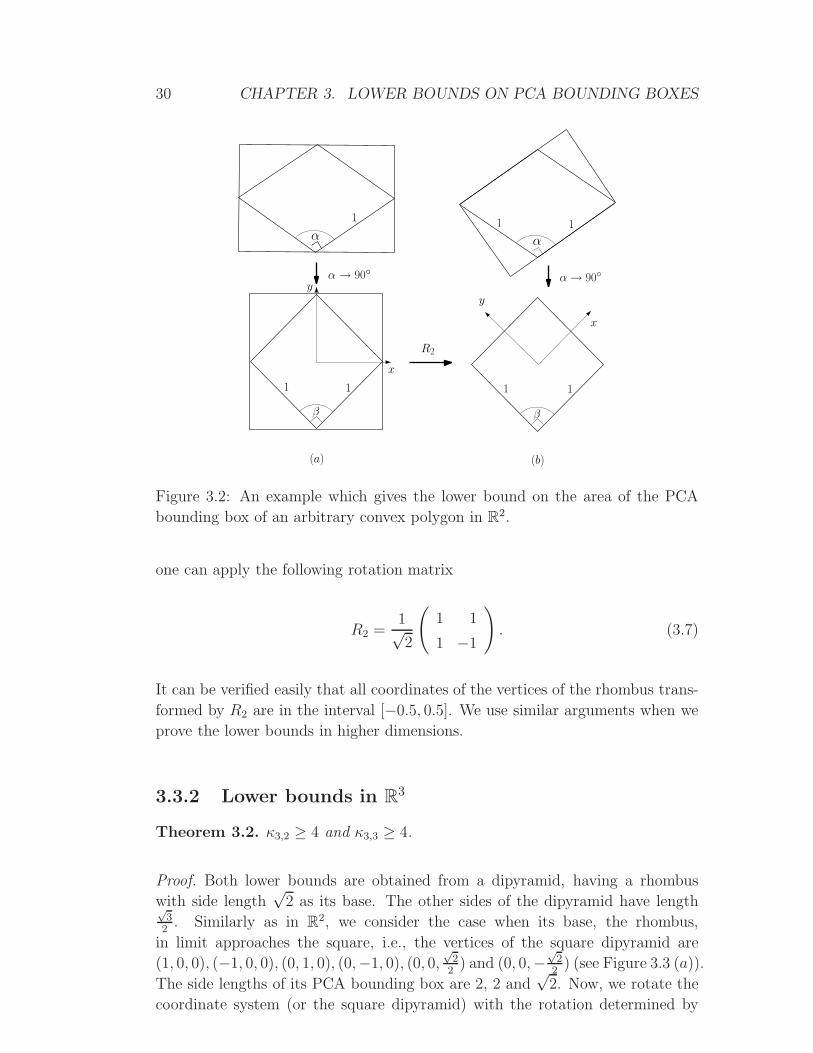
Theorem 3.1. κ2,1 ≥ 2 and κ2,2 ≥ 2.

Proof. Both lower bounds can be derived from a rhombus. Let the side length

of the rhombus be 1. To make sure that the covariance matrix has two distinct

eigenvalues, we assume that the rhombus has an angle α > 90◦. Since the

rhombus is symmetric, its PCs coincide with its diagonals. In Figure 3.2 (b) its

optimal-area bounding boxes, for 2 different angles, α > 90◦ and β = 90◦, are

shown, and in Figure 3.2 (a) its corresponding PCA bounding boxes. When the

rhombus’ angles in limit approach 90◦, the rhombus approaches a square with side

length 1, i.e., the vertices of the rhombus in the limit are ( 1√2, 0), (− 1√

2, 0), (0, 1√

2)

and (0,− 1√2) (see Figure 3.2 (a)), and the area of its PCA bounding box is√

2 ×√

2. According to Lemma 3.1, the PCs of the rhombus are unique as long

its angles are not 90◦. This leads to the conclusion that the ratio between the

area of the PCA bounding box in Figure 3.2 (a) and the area of the optimal-area

bounding box in Figure 3.2 (b) in limit goes to 2.

Alternatively, to show that the given squared rhombus fits into a unit square,


R2

(a)

1

1 1

x

yα → 90◦

11

α

11

α → 90◦

x

y

α

β β

(b)

Figure 3.2: An example which gives the lower bound on the area of the PCA

bounding box of an arbitrary convex polygon in R2.

one can apply the following rotation matrix

R2 =1√2

(1 1

1 −1

). (3.7)

It can be verified easily that all coordinates of the vertices of the rhombus trans-

formed by R2 are in the interval [−0.5, 0.5]. We use similar arguments when we

prove the lower bounds in higher dimensions.

3.3.2 Lower bounds in R3

Theorem 3.2. κ3,2 ≥ 4 and κ3,3 ≥ 4.

Proof. Both lower bounds are obtained from a dipyramid, having a rhombus

with side length√

2 as its base. The other sides of the dipyramid have length√3

2. Similarly as in R

2, we consider the case when its base, the rhombus,

in limit approaches the square, i.e., the vertices of the square dipyramid are

(1, 0, 0), (−1, 0, 0), (0, 1, 0), (0,−1, 0), (0, 0,√

22

) and (0, 0,−√

22

) (see Figure 3.3 (a)).

The side lengths of its PCA bounding box are 2, 2 and√

2. Now, we rotate the

coordinate system (or the square dipyramid) with the rotation determined by


1

1

√

2

x

y

z2

2

√

2

2

2

y

z

x

R3

(a) (b)

Figure 3.3: An example which gives the lower bound on the volume of the PCA

bounding box of an arbitrary convex polygon in R3.

the following orthogonal matrix

R3 =

1√2

− 1√2

012

12

− 1√2

12

12

1√2

. (3.8)

It can be verified easily that the square dipyramid, after rotation with R3 fits

into the cube [−0.5, 0.5]3 (see Figure 3.3 (b)). Thus, the ratio of the volume of

the bounding box, Figure 3.3 (a), and the volume of its PCA bounding box,

Figure 3.3 (b), in limit goes to 4.

3.3.3 Lower bounds in Rd

The lower bounds, presented in this subsection, are based on the following result.

Theorem 3.3. If the dimension d of the bounding box is

(a) a power of two, or

(b) a multiply of four and at most 664,

then κd,d−1 ≥ dd/2 and κd,d ≥ dd/2.

Proof. (a) For any d = 2k, k ∈ N \ {0}, let ai be a d-dimensional vector, with

aii =√

d2

and aij = 0 for i 6= j, and let bi = −ai. We construct a d-dimensional

convex polytope Pd with vertices V = {ai,bi|1 ≤ i ≤ d}. It is easy to check

that the hyperplane orthogonal to ai is a hyperplane of reflective symmetry, and

as consequence of Lemma 3.1, ai is an eigenvector of the covariance matrix of

Pd. To ensure that all eigenvalues are different (which implies that the PCA

bounding box is unique), we add ǫi > 0 to the i-th coordinate of ai, and −ǫi

to the i-th coordinate of bi, for 1 ≤ i ≤ d, where ǫ1 < ǫ2 < · · · < ǫd. When

all ǫi, 1 ≤ i ≤ d, tend to 0, the PCA bounding box of the convex polytope


Pd converges to a hypercube with side lengths√

d, i.e., the volume of the PCA

bounding box of Pd converges to dd/2. Now, we rotate Pd, such that it fits into

the cube [−12, 1

2]d. For d = 2k, we can use a rotation matrix

Rd =1√2

(R d

2R d

2

R d2

−R d2

), (3.9)

where we start with the matrix R1 = (1). A straightforward calculation verifies

that Pd rotated with Rd fits into the cube [−0.5, 0.5]d.

(b) Before we prove this part of the theorem, we would like to note that the

derivation of Rd in (a) can be traced back to a Hadamard matrix.

A Hadamard matrix of order d × d, denoted by Hd, is a ±1 matrix with

orthogonal columns.

Alternatively, we can define Rd as

Rd =1√dHd, (3.10)

where

Hd =

(H d

2H d

2

H d2

−H d2

), (3.11)

and

H2 =

(1 1

1 −1

). (3.12)

From the construction in the proof for (a), it follows that the theorem holds

for all dimensions d for which a d × d Hadamard matrix exists. In (a), it was

shown that a Hadamard matrix always exits when d = 2k, k ∈ N\{0}. Hadamard

conjectured that a Hadamard matrix also exists when d = 4k, k ∈ N \ {0}. This

conjecture is known to be true for d ≤ 664 [23].

We can combine lower bounds from lower dimensions to get lower bounds in

higher dimensions by taking Cartesian products. If κd1 is a lower bound on the

ratio between the PCA bounding box and the optimal bounding box of a convex

polytope in Rd1 , and κd2 is a lower bound in R

d2 , then κd1 · κd2 is a lower bound

in Rd1+d2 . This observation together with the results from this section enables

us to obtain lower bounds in any dimension.

For example, for the first 12 dimensions, the lower bounds we obtain are given

in Table 3.1.

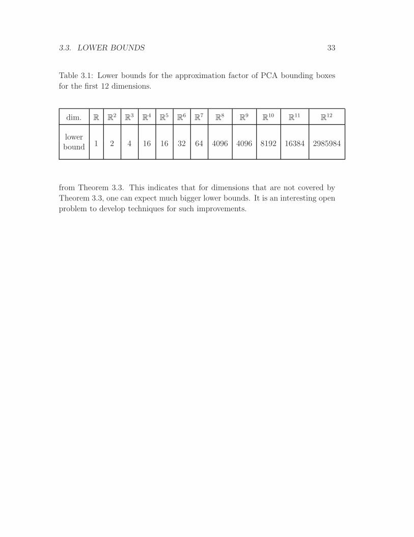
One can observe big gaps between the bounds in R7 and R

8, and between

the bounds in R11 and R

12. The bound in R7 is obtained as a product of the

lower bounds in R3 and R

4, and the bound in R11 is obtained as a product of the

lower bounds in R3 and R

8, while the bounds in R8 and R

12 are obtained directly


Table 3.1: Lower bounds for the approximation factor of PCA bounding boxes

for the first 12 dimensions.

dim. R R2

R3

R4

R5

R6

R7

R8

R9

R10

R11

R12

lowerbound 1 2 4 16 16 32 64 4096 4096 8192 16384 2985984

from Theorem 3.3. This indicates that for dimensions that are not covered by

Theorem 3.3, one can expect much bigger lower bounds. It is an interesting open

problem to develop techniques for such improvements.

Chapter 4

Upper Bounds on the Quality of

PCA Bounding Boxes

In this chapter, we present upper bounds on the approximation factors of PCA

bounding boxes in R2 and R

3. As it was shown in Proposition 3.1, the considered

bounds for discrete point sets tend to infinity. Thus, we are interested in PCA

bounding boxes for continuous point sets, especially for the convex hull of point

sets. In Proposition 3.2, it was shown that the only two cases, related to the

convex hull of the point set, when the approximation factor does not tend to

infinity, are those when the whole convex hull, or the boundary of the convex

hull are considered. The corresponding approximation factors were denoted by

κd,d and κd,d−1. In this chapter, we present upper bounds on κ2,1, κ2,2 and κ3,3.

Starting from the principle that the study of the worst case examples (es-

tablished by the known lower bounds) could give an idea how to prove upper

bounds, we make a surprising observation: Since most of the worst case exam-

ples have minimum-volume bounding boxes with unit lengths of all sides, it is

trivial that any bounding box approximates with a factor at most√

dd. Thus,

we have a trivial upper bound for all point sets with an optimal bounding box

of unit lengths of all sides. Moreover, in R2 this argument can be generalized to

a parameterized upper bound depending on the ratio η between the lengths of

the longest and the shortest side of the minimum-volume bounding box. Again,

this is not a special upper bound for the PCA-algorithm, it applies to all “tight”

bounding boxes with respect to any orthonormal coordinate system. Thus, we

need a second upper bound argument that makes use of the special properties of

PCA, and that works well when the ratio η is large. To obtain the final upper

bound we consider the lower envelop of both parameterized bounds and search

for its maximum (over all η ≥ 1).

Upper bounds in R2. The first parameterized bound in R

2 is common for

both κ2,1 and κ2,2. It depends on the parameter η. The bound is presented in

Lemma 4.1, and it is based on a simple estimation of the diameter of the point

set. It is good for a small values of the parameter η. An improvement of this

35

36 CHAPTER 4. UPPER BOUNDS ON PCA BOUNDING BOXES

bound is presented in Lemma 4.5 and it is obtained by computing the maximum

area rectangle that touches a certain rectangle.

The second parameterized bounds on κ2,1 and κ2,2 are presented in Lem-

mas 4.4 and 4.9, respectively. Both are good for big values of the parameter

η. The essence of deriving these bounds is an estimation of the distance of the

continuous point set to its best fitting line. However, the techniques used to

obtain the estimations differ for κ2,1 and for κ2,2. For κ2,1, we exploit arguments

from discrete geometry (Lemmas 4.2 and 4.3), while for κ2,2 we use ideas from

integral calculus (Theorems 4.3 and 4.4).

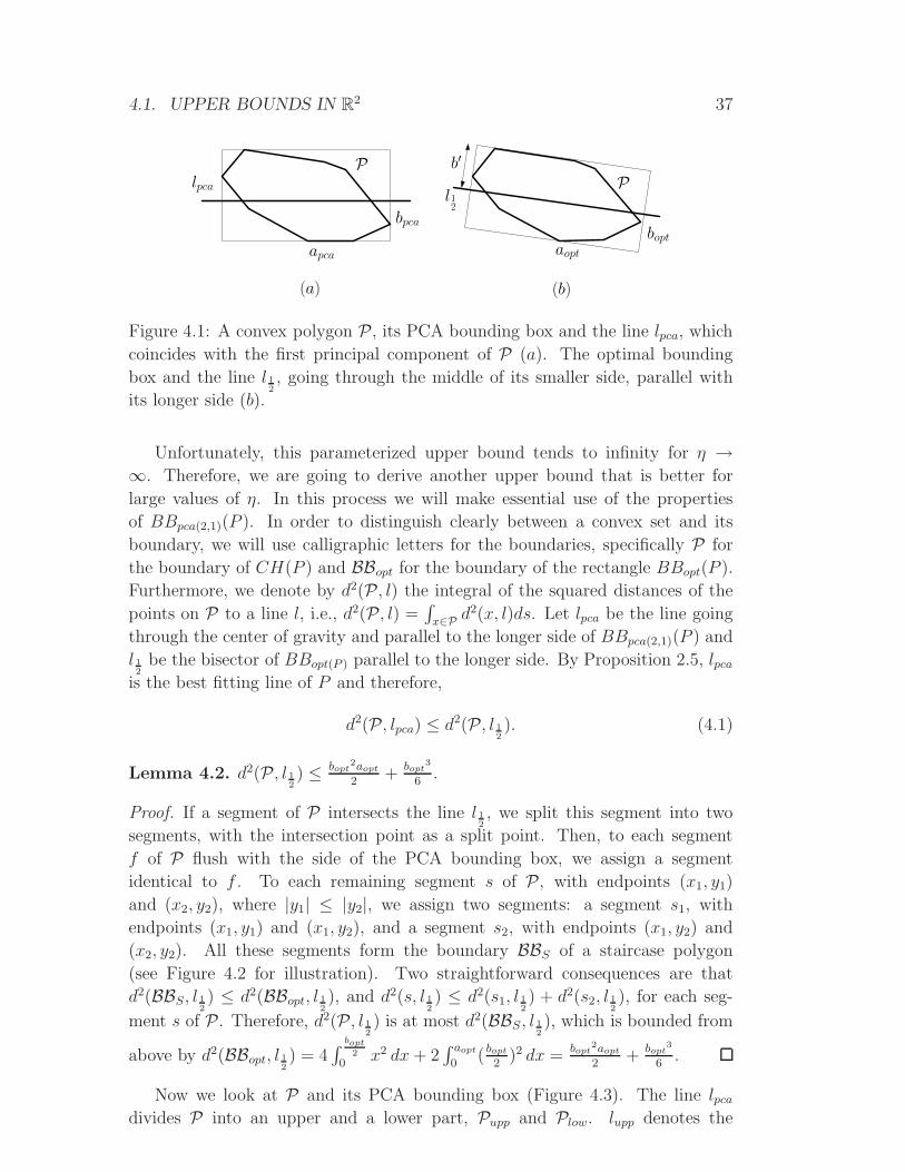
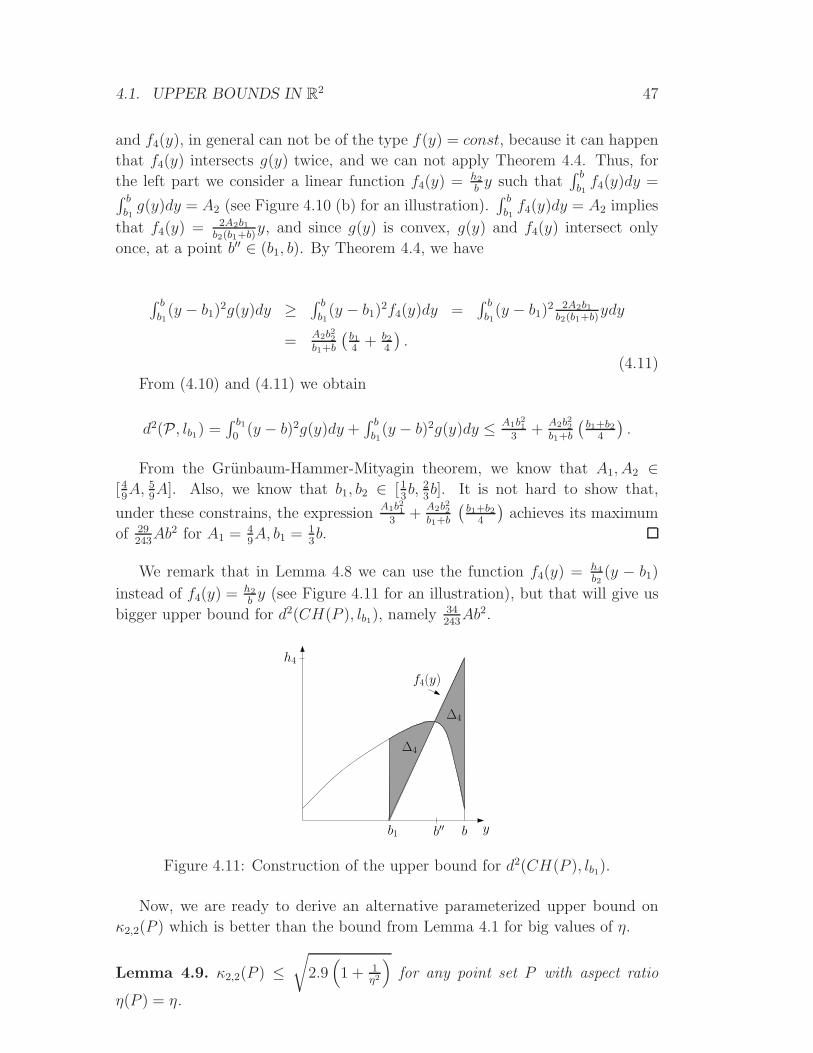
An upper bound in R3. We present an upper bound on κ3,3. We follow

the ideas from the derivation of the upper bounds on κ2,2. However, in R3 there

are two main differences with respect to R2. First, the density function of the

convex hull in R3 (see Section 4.2.1 for the definition) is not convex. Instead of

convexity, another property of the density function (described in Proposition 4.1)

is used. Second, the higher dimensionality of the problem requests an additional

relation between the sides lengths of the minimum-volume bounding box and

PCA bounding box, which is obtained in Lemma 4.13.

4.1 Upper Bounds in R2

4.1.1 An upper bound on κ2,1

Given a point set P ⊆ R2 and an arbitrary bounding box BB(P ) we will denote

the two side lengths by a and b, where a ≥ b. We are interested in the side

lengths aopt(P ) ≥ bopt(P ) and apca(P ) ≥ bpca(P ) of BBopt(P ) and BBpca(2,1)(P ),

see Figure 4.1. The parameters α = α(P ) = apca(P )/aopt(P ) and β = β(P ) =

bpca(P )/bopt(P ) denote the ratios between the corresponding side lengths. Hence,

we have κ2,1(P ) = α(P ) · β(P ). If the relation to P is clear, we will omit the

reference to P in the notations introduced above.

Since the side lengths of any bounding box are bounded by the diameter of

P , we can observe that in general bpca(P ) ≤ apca(P ) ≤ diam(P ) ≤√

2aopt(P ),

and in the special case when the optimal bounding box is a square κ2,1(P ) ≤ 2.

This observation can be generalized, introducing an additional parameter η(P ) =

aopt(P )/bopt(P ).

Lemma 4.1. κ2,1(P ) ≤ η + 1η

and κ2,2(P ) ≤ η + 1η

for any point set P with

fixed aspect ratio η(P ) = η.

Proof. We have for both apca and bpca the upper bound diam(P ) ≤√

a2opt + b2

opt

= aopt

√1 + 1

η2 . Replacing aopt by η · bopt in the bound on bpca we obtain αβ ≤

η(√

1 + 1η2

)2

= η + 1η.

4.1. UPPER BOUNDS IN R2 37

apca

bpca

lpca

P

l1

2

bopt

aopt

P

b′

(a) (b)

Figure 4.1: A convex polygon P, its PCA bounding box and the line lpca, which

coincides with the first principal component of P (a). The optimal bounding

box and the line l 12, going through the middle of its smaller side, parallel with

its longer side (b).

Unfortunately, this parameterized upper bound tends to infinity for η →∞. Therefore, we are going to derive another upper bound that is better for

large values of η. In this process we will make essential use of the properties

of BBpca(2,1)(P ). In order to distinguish clearly between a convex set and its

boundary, we will use calligraphic letters for the boundaries, specifically P for

the boundary of CH(P ) and BBopt for the boundary of the rectangle BBopt(P ).

Furthermore, we denote by d2(P, l) the integral of the squared distances of the

points on P to a line l, i.e., d2(P, l) =∫

x∈P d2(x, l)ds. Let lpca be the line going

through the center of gravity and parallel to the longer side of BBpca(2,1)(P ) and

l 12

be the bisector of BBopt(P ) parallel to the longer side. By Proposition 2.5, lpca

is the best fitting line of P and therefore,

d2(P, lpca) ≤ d2(P, l 12). (4.1)

Lemma 4.2. d2(P, l 12) ≤ bopt

2aopt

2+ bopt

3

6.

Proof. If a segment of P intersects the line l 12, we split this segment into two

segments, with the intersection point as a split point. Then, to each segment

f of P flush with the side of the PCA bounding box, we assign a segment

identical to f . To each remaining segment s of P, with endpoints (x1, y1)

and (x2, y2), where |y1| ≤ |y2|, we assign two segments: a segment s1, with

endpoints (x1, y1) and (x1, y2), and a segment s2, with endpoints (x1, y2) and

(x2, y2). All these segments form the boundary BBS of a staircase polygon

(see Figure 4.2 for illustration). Two straightforward consequences are that

d2(BBS, l 12) ≤ d2(BBopt, l 1

2), and d2(s, l 1

2) ≤ d2(s1, l 1

2) + d2(s2, l 1

2), for each seg-

ment s of P. Therefore, d2(P, l 12) is at most d2(BBS, l 1

2), which is bounded from

above by d2(BBopt, l 12) = 4

∫ bopt

20

x2 dx + 2∫ aopt

0( bopt

2)2 dx = bopt

2aopt

2+ bopt

3

6.

Now we look at P and its PCA bounding box (Figure 4.3). The line lpca

divides P into an upper and a lower part, Pupp and Plow. lupp denotes the


l1

2

aopt

bopt

BBS P

Figure 4.2: The convex polygon P, its optimal bounding box, and the staircase

polygon BBS (depicted dashed).

Tupp

Tlow

U1 L1

apca

bpca

lpca

Pb′

L2U2

U3

L3

a1a2

b1 b2

Figure 4.3: The convex polygon P, its PCA bounding box, and a construction

for a lower bound on d2(P, lpca).

orthogonal projection of Pupp onto lpca, with U1 and U2 as its extreme points,

and llow denotes the orthogonal projection of Plow onto lpca, with L1 and L2

as its extreme points. Tupp = △(U1U2U3) is a triangle inscribed in the upper

part of the PCA bounding box (the part above lpca), where point U3 lies on the

intersection of Pupp with the upper side of the PCA bounding box. Analogously,

Tlow = △(L1L2L3) is a triangle inscribed in the lower part of the PCA bounding

box (the part below lpca).

Lemma 4.3.

d2(P, lpca) ≥ d2(Tupp, lpca) + d2(Tlow, lpca).

Proof. Let Q denote a chain of segments of P, which does not touch the longer

side of the PCA bounding box, and whose one endpoint lies on the smaller

side of the PCA bounding box, and the other endpoint on the line lpca. We

reflect Q at the line supporting the side of the PCA bounding box touched by

Q. All such reflected chains of segments, together with the rest of P, form two

polylines: P ′upp and P ′

low (see Figure 4.4 for illustration). As a consequence,

to each of the sides of the triangles Tlow and Tupp, L1L3, L2L3, U1U3, U2U3,

we have a corresponding chain of segments R as shown in the two cases in

Figure 4.5. In both cases d2(t, lpca) ≤ d2(R, lpca). Namely, we can parametrize

both curves, R and t, starting at the common endpoint A that is furthest from

lpca. By comparing two points with the same parameter (distance from A along

the curve) we see that the point on t always has a smaller distance to lpca than


Tupp

Tlow

apca

bpca

lpca

P ′upp

P ′low

P

Figure 4.4: Two polylines P ′upp and P ′

low (depicted dashed) formed from P.

lpca lpca

R Rt t

(a) (b)

A A

Figure 4.5: Two types of chains of segments (depicted dashed and denoted by

R), and their corresponding triangles’ edges (depicted solid and denoted by t).

The base-point of t corresponds to the most left point of Tupp from Figure 4.3

and Figure 4.4.

the corresponding point on R. In addition t is shorter, and some parts of R have

no match on t.

Consequently, d2(P ′, lpca) ≥ d2(Tupp

⋃Tlow, lpca) = d2(Tupp, lpca)+d2(Tlow, lpca),

and since d2(P ′, lpca) = d2(P, lpca) = d2(Pupp

⋃Plow, lpca), the proof is com-

pleted.

Since P is convex, the following relations hold:

|lupp| ≥b′

bpcaapca, and |llow| ≥

bpca − b′

bpcaapca. (4.2)

The value

d2(Tupp, lpca) =∫√a2

1+b′2

0( α√

a21+b′2

b′)2 dα +∫√a2

2+b′2

0( α√

a22+b′2

b′)2 dα

= b′2

3(√

a21 + b′2 +

√a2

2 + b′2)

is minimal when a1 = a2 = |lupp|2

. With (4.2) we get

d2(Tupp, lpca) ≥b′3

3bpca

√a2

pca + 4b2pca.

Analogously, we have for the lower part:

d2(Tlow, lpca) ≥(bpca − b′)3

3bpca

√a2

pca + 4b2pca.


The sum d2(Tupp, lpca) + d2(Tlow, lpca) is minimal when b′ = bpca

2. This, together

with Lemma 4.3, gives:

d2(P, lpca) ≥b2pca

12

√a2

pca + 4b2pca. (4.3)

Combining (4.1), (4.3) and Lemma 4.2 we have:

1

2aoptb

2opt +

1

6b3opt ≥

b2pca

12

√a2

pca + 4b2pca ≥

b2pca

12apca. (4.4)

Replacing aopt with ηbopt on the left side, b2pca with β2b2

opt and apca with αaopt =

αηbopt on the right side of (4.4), we obtain:(

η

2+

1

6

)b3opt ≥

β2 α η

12b3opt

which implies

β ≤√

6η + 2

α η.

This gives the second upper bound on κ2,1(P ) for point sets with parameter η:

α β ≤√

(6η + 2)α

η≤

√6η + 2

η

√1 +

1

η2. (4.5)

Lemma 4.4. κ2,1(P ) ≤√

6η+2η

√1 + 1

η2 for any point set P with fixed aspect

ratio η(P ) = η.

This implies the final result of this subsection.

Theorem 4.1. The PCA bounding box of a point set P in R2 computed over the

boundary of CH(P ) has a guaranteed approximation factor κ2,1 ≤ 2.737.

Proof. The theorem follows from the combination of the two parameterized

bounds from Lemma 4.1 and Lemma 4.4 proved above:

κ2,1 ≤ supη≥1

min

η +

1

η,

√6η + 2

η

√1 +

1

η2

.

It is easy to check that the supremum s ≈ 2.736 is obtained for η ≈ 2.302.

4.1.2 An improved upper bound on κ2,1

An improvement of the upper bound on κ2,1 is obtained by providing better

upper bound on κ2,1 for big η than that from Lemma 4.1.

Given two rectangles R1 and R2 in R2, we say that R2 touches R1 if the

intersection of each side of R2 with R1 is a corner of R1, or a side of R1. Note

that in the latter case, R1 and R2 are identical.


Lemma 4.5. Let R1 be a rectangle in R2, with side’s lengths a and b, such that

a = ηb, η ≥ 1. Then, the area of the maximum-area rectangle that touches R1 is(η+1)2 b2

2.

Proof. Let R2 denote the maximum-area rectangle that touches R1. Due to

Thales theorem, the corners of R2 must lie on the half-circles built above each

side of R1. See Figure 4.6 for an illustration. The area of R2 equals to the area

R2

R2

(a) (b)

R1 R1

d

a

b

α

α

α

α

Figure 4.6: (a) A rectangle R1 and a touching rectangle R2 of R1. (b) The

maximum-area touching rectangle R2 of R1.

of R1 plus the area of the four similar triangles (the triangles with angle α in

Figure. 4.6). Then

area(R2) = ab + a2 sin α cos α + b2 sin α cos α

= ab + (a2 + b2)sin 2α

2.

This expression has maximal value for α = π4, namely (a+b)2

2. Since a = ηb, we

finally have that the maximal area of R2 is (η+1)2 b2

2.

Lemma 4.6. κ2,1(P ) ≤ (η+1)2

2 ηand κ2,2(P ) ≤ (η+1)2

2 ηfor any point set P with

fixed aspect ratio η(P ) = η.

Proof. For a point set P with fixed aspect ratio η we have that area(BBopt(P )) =

aoptbopt = ηbopt2. Denote by BBmax the maximum-area rectangle that touches

BBopt. By Lemma 4.5 it follows that area(BBmax) = (η+1)2 bopt2

2. Thus, we have

area(BBpca(P ))

area(BBopt(P ))≤ area(BBmax(P ))

area(BBopt(P ))=

(η + 1)2 bopt2

2 η bopt2 =

(η + 1)2

2 η.


Theorem 4.2. The PCA bounding box of a point set P in R2 computed over

CH(P ) has a guaranteed approximation factor κ2,1 ≤ 2.654.


bounds from Lemma 4.4 and Lemma 4.6:

κ2,1 ≤ supη≥1

min

(η + 1)2

2 η,

√6η + 2

η

√1 +

1

η2

.

The supremum for the expression above occurs at 2.6535 for η ≈ 2.970.

Although these results concern a continuous PCA version, the proofs are

mainly based on arguments from discrete geometry. In contrast to that, the

upper bound proofs for κ2,2 and κ3,3, presented in the next two subsections,

essentially make use of integral calculus.


lopt

bopt

aopt

CH(P )

apca

bpca

lpca CH(P )

c c

BBpca(2,2)(P ) BBopt(P )

(a) (b)

Figure 4.7: A convex hull of the point set P , its PCA bounding box (a) and its

optimal bounding box(b).

First, we note that due to Lemma 4.1, we already have a parameterized upper

bound on κ2,2. Since this bound tends to infinity for η → ∞, we are going to

derive another upper bound on κ2,2 that is better for large values of η. We

derive such a bound by finding a constant that bounds β from above. In this

process we will make essential use of the properties of BBpca(2,2)(P ). We denote

by d2(CH(P ), l) the integral of the squared distances of the points on CH(P )

to a line l, i.e.,

d2(CH(P ), l) =

∫

s∈CH(P )

d2(s, l)ds.

Let lpca be the line going through the center of gravity, parallel to the longer side

of BBpca(2,2)(P ), and lopt be the line going through the center of gravity, parallel


to the longer side of BBopt(P ) (see Figure 4.7). By Proposition 2.5, lpca is the

best fitting line of P and therefore,

d2(CH(P ), lpca) ≤ d2(CH(P ), lopt). (4.6)

We obtain an estimate of β by determining a lower bound on d2(CH(P ), lpca)

that depends on bpca, and an upper bound on d2(CH(P ), lopt) that depends on

bopt. Having an arbitrary bounding box of CH(P ) (with side lengths a and b,

a ≥ b) the area of CH(P ) can be expressed as

A = A(CH(P )) =

∫ b

0

∫ a

0

χCH(P )(x, y)dxdy =

∫ b

0

g(y)dy,

where χCH(P )(x, y) is the characteristic function of CH(P ) defined as

χCH(P )(x, y) =

1 (x, y) ∈ CH(P )

0 (x, y) /∈ CH(P ),

and g(y) =∫ a

0χCH(P )(x, y)dx is the length of the intersection of CH(P ) with a

horizontal line at height y. In the following we call g(y) the density function of

CH(P ) for computing the area with the integral∫ b

0g(y)dy. Note that g(y) is

continuous and convex in the interval [0, b] (see Figure 4.8 for an illustration).

Let b1 denote the y-coordinate of the center of gravity of CH(P ). The line lb1

ybb1

A1 A2A

g(y)

Figure 4.8: Density function g(y) of the convex hull of a point set in R2.

(y = b1) divides the area of CH(P ) into A1 and A2.

Theorem 4.4, which is derived from the generalized first mean value theorem

of integral calculus (Theorem 4.3), is our central technical tool in derivation of

the lower and the upper bound on d2(CH(P ), lb1).

Theorem 4.3. (Generalized first mean value theorem of integral calculus)

If h(x) and g(x) are continuous functions on the interval [a, b], and if g(x) does


not change its sign in the interval, then there is a ξ ∈ (a, b) such that

∫ b

a

h(x)g(x)dx = h(ξ)

∫ b

a

g(x)dx.

Theorem 4.4. Let f(x) and g(x) be positive continuous functions on the interval

[a, b] with∫ b

af(x)dx =

∫ b

ag(x)dx, and assume that there is some c ∈ [a, b] such

that f(x) ≤ g(x), for all x ≤ c and f(x) ≥ g(x), for all x ≥ c. Then

∫ b

a

(x − b)2f(x)dx ≤∫ b

a

(x − b)2g(x)dx and

∫ b

a

(x − a)2f(x)dx ≥∫ b

a

(x − a)2g(x)dx.

Proof. We start from the assumptions∫ b

af(x)dx =

∫ b

ag(x)dx and f(x) ≤ g(x)

for all x ≤ c and f(x) ≥ g(x) for all x ≥ c. Thus,

∫ c

a

(g(x) − f(x))dx =

∫ b

c

(f(x) − g(x))dx = ∆ (4.7)

and the integrands on both sides are nonnegative. Applying Theorem 4.3 to the

following integrals we obtain∫ c

a

(x − b)2(g(x) − f(x))dx = (ξ1 − b)2

∫ c

a

(g(x) − f(x))dx = (ξ1 − b)2∆,

and∫ b

c

(x − b)2(f(x) − g(x))dx = (ξ2 − b)2

∫ b

c

(f(x) − g(x))dx = (ξ2 − b)2∆,

for some ξ1 ∈ [a, c] and ξ2 ∈ [c, b]. Therefore,

∫ c

a

(x−b)2(g(x)−f(x))dx = (ξ1−b)2∆ ≥ (ξ2−b)2∆ =

∫ b

c

(x−b)2(f(x)−g(x))dx.

It follows that∫ b

a

(x−b)2(g(x)−f(x))dx =

∫ c

a

(x−b)2(g(x)−f(x))dx−∫ b

c

(x−b)2(f(x)−g(x))dx ≥ 0,

which proves the first claim

∫ b

a

(x − b)2f(x)dx ≤∫ b

a

(x − b)2g(x)dx.

The proof of the second claim follows by symmetry.

The following theorem was discovered independently by Grunbaum [15] and

Hammer (unpublished manuscript), and later rediscovered by Mityagin [31]. We

use it to prove a lower and an upper bound of the variance d2(CH(P ), lb1).


Theorem 4.5 (Grunbaum-Hammer-Mityagin). Let K be a compact convex set

in Rd with non-empty interior and centroid µ. Assume that the d-dimensional

volume of K is one, that is, Vold(K) = 1. Let H be any (d-1)-dimensional

hyperplane passing through µ with corresponding half-spaces H+ and H−. Then,

min{Vold(K ∩ H+),Vold(K ∩ H−)} ≥(

d

d + 1

)d

.

Moreover, the bound ( dd+1

)d is best possible.

Lemma 4.7. The variance d2(CH(P ), lb1) is bounded from below by 10243

Ab2.

Proof. We split the integral∫ b

0(y − b1)

2g(y)dy at b1 (recall that b1 is the y-

coordinate of the center of gravity of CH(P )), and prove lower bounds on

both parts in the following way: For the left part consider the linear function

f1(y) = h1

b1y such that

∫ b10

f1(y)dy =∫ b1

0g(y)dy = A1 (see Figure 4.9 (a) for an

illustration). From∫ b10

f1(y)dy = A1, it follows that f1(y) = 2A1yb21

. Since g(y) is

convex, g(y) and f1(y) intersect only once, at a point b′ ∈ (0, b1).

(b)

ybb1

A2

f2(y)

∆2

∆2

b′′

h2

(a)

ybb1

A1

f1(y)

b′

h1

∆1

∆1

Figure 4.9: Construction of the lower bound on d2(CH(P ), lb1).

By Theorem 4.4, we have

∫ b1

0

(y − b1)2g(y)dy ≥

∫ b1

0

(y − b1)2f1(y)dy =

∫ b1

0

(y − b)2 2A1

b12 dy =

A1b21

6. (4.8)

Analogously, for the right part consider the linear function f2(y) = h2

b1−b(y− b) =

h2

−b2(y − b) such that

∫ b

b1f2(y)dy =

∫ b

b1g(y)dy = A2 (see Figure 4.9 (b) for an

illustration). From∫ b

b1f2(y)dy = A2, it follows that f2(y) = 2A2

b22(y − b). Since

g(y) is convex, g(y) and f2(y) intersect only once, at a point b′′ ∈ (b1, b). By


Theorem 4.4, we have that

∫ b

b1(y − b1)

2g(y)dy ≥∫ b

b1(y − b1)

2f2(y)dy =∫ b

b1(y − b1)

2 2A2

(b−b1)2(y − b1)dy

=A2b22

6.

(4.9)

From (4.8) and (4.9) we obtain that

d2(CH(P ), lb1) =∫ b10

(y − b1)2g(y)dy +

∫ b

b1(y − b1)

2g(y)dy ≥ A1b216

+A2b22

6.

From the Grunbaum-Hammer-Mityagin theorem, we know that A1, A2 ∈ [49A, 5

9A].

Also, we know that b1, b2 ∈ [13b, 2

3b]. It is not hard to show that, under these con-

strains, the expressionA1b21

6+

A2b216

achieves its minimum of 10243

Ab2 for A1 =49A, b1 = 5

9b or A1 = 5

9A, b1 = 4

9b.

Lemma 4.8. The variance d2(CH(P ), lb1) is bounded from above by 29243

Ab2.

Proof. Without loss of generality, we can assume that g(y) has its maximum in

[b1, b]. We split the integral∫ b

0(y − b1)

2g(y)dy at b1, and prove upper bounds

for both parts in the following way. For the left part consider a linear function

f3(y) = h3 such that∫ b10

f3(y)dy =∫ b10

g(y)dy = A1 (see Figure 4.10 (a) for an

illustration). This implies that f3(y) = A1

b1, and since g(y) is convex, g(y) and

(a)

ybb1

f3(y)∆3

∆3

h3

b′

(b)

b′′ ybb1

f4(y)

∆4 ∆4

h4

Figure 4.10: Construction of the upper bound for d2(CH(P ), lb1).

f3(y) intersect only once, at a point b′ ∈ (b1, b). By Theorem 4.4, we have

∫ b10

(y − b1)2g(y)dy ≤

∫ b10

(y − b1)2f3(y)dy =

∫ b10

(y − b1)2 A1

b1dy =

A1b213

. (4.10)

Now, we are looking for an appropriate function f4(y) to derive an upper bound of

the second part of the integral∫ b

0(y− b1)

2g(y)dy. Note that both functions f3(y)


and f4(y), in general can not be of the type f(y) = const, because it can happen

that f4(y) intersects g(y) twice, and we can not apply Theorem 4.4. Thus, for

the left part we consider a linear function f4(y) = h2

by such that

∫ b

b1f4(y)dy =∫ b

b1g(y)dy = A2 (see Figure 4.10 (b) for an illustration).

∫ b

b1f4(y)dy = A2 implies

that f4(y) = 2A2b1b2(b1+b)

y, and since g(y) is convex, g(y) and f4(y) intersect only

once, at a point b′′ ∈ (b1, b). By Theorem 4.4, we have

∫ b

b1(y − b1)

2g(y)dy ≥∫ b

b1(y − b1)

2f4(y)dy =∫ b

b1(y − b1)

2 2A2b1b2(b1+b)

ydy

=A2b22b1+b

(b14

+ b24

).

(4.11)

From (4.10) and (4.11) we obtain

d2(P, lb1) =∫ b10

(y − b)2g(y)dy +∫ b

b1(y − b)2g(y)dy ≤ A1b21

3+

A2b22b1+b

(b1+b2

4

).

From the Grunbaum-Hammer-Mityagin theorem, we know that A1, A2 ∈[49A, 5

9A]. Also, we know that b1, b2 ∈ [1

3b, 2

3b]. It is not hard to show that,

under these constrains, the expressionA1b21

3+

A2b22b1+b

(b1+b2

4

)achieves its maximum

of 29243

Ab2 for A1 = 49A, b1 = 1

3b.

We remark that in Lemma 4.8 we can use the function f4(y) = h4

b2(y − b1)

instead of f4(y) = h2

by (see Figure 4.11 for an illustration), but that will give us

bigger upper bound for d2(CH(P ), lb1), namely 34243

Ab2.

ybb1

f4(y)

∆4

∆4

h4

b′′

Figure 4.11: Construction of the upper bound for d2(CH(P ), lb1).

Now, we are ready to derive an alternative parameterized upper bound on

κ2,2(P ) which is better than the bound from Lemma 4.1 for big values of η.

Lemma 4.9. κ2,2(P ) ≤√

2.9(1 + 1

η2

)for any point set P with aspect ratio

η(P ) = η.


Proof. Applying Lemma 4.7 and Lemma 4.8 in (4.6) we obtain

10

243Ab2

pca ≤ d2(P, lpca) ≤ d2(P, lopt) ≤29

243Ab2

opt. (4.12)

From (4.12) it follows that β = bpca

bopt≤

√2.9. We have for apca the upper bound

diam(P ) ≤√

a2opt + b2

opt = aopt

√1 + 1

η2 . From this, it follows that α ≤√

1 + 1η2 .

Putting this together, we obtain αβ ≤√

2.9(1 + 1

η2

).





κ2,2 ≤ supη≥1

{min

(η +

1

η,

√2.9

(1 +

1

η2

))}.

It is easy to check that the supremum s ≈ 2.1038 is obtained for η ≈ 1.3784.

4.1.4 An improved upper bound on κ2,2

An improvement of the upper bound on κ2,2 is obtained by applying the better

upper bound on κ2,2 for big η from Lemma 4.6 instead of applying the bound

from Lemma 4.1.





κ2,2 ≤ supη≥1

{min

((η + 1)2

2 η,

√2.9

(1 +

1

η2

))}.

The supremum of the above expression occurs at 2.0694044 for η ≈ 1.4483691.

4.2 An upper bound in R3


Some of the techniques used here are similar to those used in Subsection 4.1.3

where we derive an upper bound on κ2,2. One essential difference is that for

the upper bound on κ3,3, we additionally need a bound for the ratio of the

4.2. AN UPPER BOUND IN R3 49

middle sides of BBpca(3,3)(P ) and BBopt(P ), which we derive from the relation

in Lemma 4.13.

Given a point set P ⊆ R3 and an arbitrary bounding box BB(P ), we will

denote the three side lengths of BB(P ) by a,b and c, where a ≥ b ≥ c. We are

interested in the side lengths aopt ≥ bopt ≥ copt and apca ≥ bpca ≥ cpca of BBopt(P )

and BBpca(3,3)(P ). The parameters α = α(P ) = apca/aopt, β = β(P ) = bpca/bopt

and γ = γ(P ) = cpca/copt denote the ratios between the corresponding side

lengths. Hence, we have κ3,3(P ) = α · β · γ.

Since the side lengths of any bounding box are bounded by the diameter of

P , we can observe that in general cpca ≤ bpca ≤ apca ≤ diam(P ) ≤√

3aopt, and in

the special case when the optimal bounding box is a cube κ3,3(P ) ≤ 3√

3. This

observation can be generalized, introducing two additional parameters η(P ) =

aopt/bopt and θ(P ) = aopt/copt.

Lemma 4.10. κ3,3(P ) ≤ η θ(1 + 1

η2 + 1θ2

) 32

for any point set P with aspect

ratios η(P ) = η and θ(P ) = θ.

Proof. We have for apca, bpca and cpca the upper bound diam(P ) ≤√

a2opt + b2

opt + c2opt

= aopt

√1 + 1

η2 + 1θ2 . Thus, α β γ ≤ apca bpca cpca

aopt bopt copt≤

a3opt

(1+ 1

η2

) 32

aoptboptcopt. Replacing aopt in

the nominator once by η bopt and once by θ copt we obtain κ3,3(P ) ≤ η θ(1 + 1

η2 + 1θ2

) 32.

Unfortunately, this parameterized upper bound tends to infinity for η → ∞ or

θ → ∞. Therefore, we are going to derive another upper bound that is better for

large values of η and θ. We derive such a bound by finding constants that bound

β and γ from above. In this process we will make essential use of the properties of

BBpca(3,3)(P ). We denote by d2(CH(P ), H) the integral of the squared distances

of the points on CH(P ) to a plane H , i.e., d2(CH(P ), H) =∫

s∈CH(P )d2(s, H)ds.

Let Hpca be the plane going through the center of gravity, parallel to the side

apca × bpca of BBpca(3,3)(P ), and Hopt be the bisector of BBopt(P ) parallel to the

side aopt × bopt. By Proposition 2.5, Hpca is the best fitting plane of P and

therefore,

d2(CH(P ), Hpca) ≤ d2(CH(P ), Hopt). (4.13)

We obtain an estimation for γ by determining a lower bound on d2(CH(P ), Hpca)

that depends on cpca, and an upper bound on d2(CH(P ), Hopt) that depends on

copt. Having an arbitrary bounding box of CH(P ) (with side lengths a, b, and

c, a ≥ b ≥ c), we denote by Hab the plane going through the center of gravity,

parallel to the side a × b. The volume of CH(P ) can be expressed as

V = V (CH(P )) =∫ c

0

∫ b

0

∫ a

0χCH(P )(x, y, z)dxdydz =

∫ c

0g(z)dz,


where χCH(P )(x, y, z) is the characteristic function of CH(P ) defined as

χCH(P )(x, y, z) =

1 (x, y, z) ∈ CH(P )

0 (x, y, z) /∈ CH(P ),

and g(z) =∫ b

0

∫ a

0χCH(P )(x, y, z)dxdy is the area of the intersection of CH(P )

with the horizontal plane at height z. As before we call g(z) the density function

of CH(P ). Let c1 denote the z-coordinate of the center of gravity of CH(P ). The

line lc1 (y = c1) divides the volume of CH(P ) into V1 and V2 (see Figure 4.12 (a)

for an illustration).

g(z)

zcc1

V1 V2V

Figure 4.12: Density function g(y) of the convex hull of a point set in R3.

Note that g(z) is continuous, but in general not convex in the interval [0, b].

Therefore, we cannot use linear functions to derive a lower and an upper bound

on the function d2(CH(P ), Hab), as we did in Subsection 4.1.3, because a linear

function can intersect g(z) more than once, and we cannot apply Theorem 4.4.

We will show that instead of linear functions, quadratic functions can be used.

Proposition 4.1. Let g(z) be the density function of CH(P ) defined as above,

and let f(z) = kz2 be the parabola such that∫ c10

f(z)dz =∫ c10

g(z)dz. Then,

∃c0 ∈ [0, c1] such that f(z) ≤ g(x) for all z ≤ c0 and f(z) ≥ g(z) for all z ≥ c0.

Proof. We give a constructive proof. Let c0 := inf { d |∀z ∈ [d, c1] g(z) ≤ f(z)}.If c0 = 0, then f(z) = g(z), and the proposition holds. If c0 > 0, then consider

the polygon which is the intersection of CH(P ) with the plane z = c0. We fix a

point p0 in CH(P ) with z-coordinate 0 and construct a pyramid Q by extending

all rays from p0 through the polygon up to the plane z = c1 (see Figure 4.13 for

an illustration). Since, f(c0) = g(c0) the quadratic function f(z) is the density

function of Q. Therefore, since the part of Q below c0 is completely included in


y

z

c0

xf (c0) = g(c0)

QCH(P )

p0

c1

Figure 4.13: Construction of the intersection of f(z) and g(z).

CH(P ), we can conclude that f(z) ≤ g(z) for all z ≤ c0. On the other hand,

f(z) ≥ g(x) for all z ≥ c0 by the definition of c0.

Now, we present a lower and an upper bound on the variance d2(CH(P ), Hab),

from which we can derive a bound on γ = cpca

copt.

Lemma 4.11. The variance d2(CH(P ), Hab) is bounded from below by 7256

V c2.

Proof. We split the integral∫ c

0(z − c1)

2g(z)dz at c1, and prove upper bounds

on both parts in the following way: For the left part consider the parabola

f1(z) = h1

c21z2 such that

∫ c10

f1(z)dz =∫ c10

g(z)dz = V1 (see Figure 4.14 (a) for an

illustration). From∫ c10

f1(z)dz = V1 we have that f1(z) = 3V1

c31z2. Since f1(z) and

g(z) define the same volume on the interval [0, c1], they must intersect, and by

Proposition 4.1 we know that if f1(z) 6= g(z), then they can intersect only once,

at a point c′ ∈ (0, c1). Under these conditions, we can apply Theorem 4.4, and

obtain

∫ c10

(z − c1)2g(z)dz ≥

∫ c10

(z − c1)2f1(z)dz =

∫ c10

(z − c1)2 3V1

c31z2dz =

V1c2110

.

(4.14)

Analogously, for the right part consider the parabola f2(z) = h2

(c1−c)2(z − c)2 =

h2

c22(z − c)2 such that

∫ c

c1f2(y)dy =

∫ c

c1g(z)dz = V2 (see Figure 4.14 (b) for an

illustration). From∫ c

c1f2(y)dy = V2 we have that f1(z) = 3V2

c32(z− c)2. By similar

arguments as above in the case of f1(z), we can show that g(z) and f2(z) intersect

only once, at a point c′′ ∈ (c1, c). Applying Theorem 4.4 we have that

∫ c

c1(z − c1)

2g(z)dz ≥∫ c

c1(z − c1)

2f2(z)dz =∫ c

c1(z − c1)

2 3V2

c32(z − c)2dz

=V2c2210

.

(4.15)

From (4.14) and (4.15) we obtain that

d2(CH(P ), Hab) =∫ c10

(z − c1)2g(z)dz +

∫ c

c1(z − c1)

2g(z)dz ≥ V1c2110

+V2c2210

.


(a)

f1(z)

zcc1

h1

c′

∆1

∆1

(b)

f2(z)

zcc1

∆2

∆2

h2

c′′

Figure 4.14: Construction of the lower bound on d2(CH(P ), Hab)

From the Grunbaum-Hammer-Mityagin theorem, we know that V1, V2 ∈ [2764

V, 3764

V ].

Also, we know that c1, c2 ∈ [14c, 3

4c]. It is not hard to show that, under these

constrains, the expressionV1c2110

+V2c2210

achieves its minimum of 7256

V c2 for V1 =2764

V, c1 = 34c or V1 = 37

64V, c1 = 1

4c.

Lemma 4.12. The variance d2(CH(P ), Hab) is bounded from above by 1272971680

V c2.

Proof. Without loss of generality, we can assume that g(z) has its maximum in

[c1, c]. We split the integral∫ c

0(z − c1)

2g(z)dz at c1, and prove upper bounds for

both parts in the following way: For the left part consider the linear function

f3(z) = h3 such that∫ c10

f3(z)dz =∫ c10

g(z)dz = V1 (see Figure 4.15 (a) for an

illustration).

(b)

f4(z)

zcc1

∆4 ∆4

h4

c′′

(a)

f3(z)

zcc1

h3

c′

∆3

∆3

Figure 4.15: Construction of the upper bound on d2(CH(P ), Hab)

From∫ c10

f3(z)dz = V1 we have that f3(z) = V1

c1. Since f3(z) is constant, it


intersects g(z) only once, at a point c′ ∈ (c1, c). By Theorem 4.4, we have that

∫ c10

(z − c1)2g(z)dz ≤

∫ c10

(z − c1)2f3(z)dz =

∫ c10

(z − c1)2 V1

c1dz =

V1c213

. (4.16)

Now, we are looking for an appropriate function f4(z) to derive an upper bound

on the second part of the integral∫ z

0(z − c1)

2g(z)dz. Note that both functions

f3(z) and f4(z), in general can not be of the type f(y) = const, which give us the

best upper bound, because it can happen that f4(z) intersects g(z) twice, and

we can not apply Theorem 4.4. Thus, for the right part we consider the parabola

f4(z) = h4

c2z2 such that

∫ c

c1f4(z)dz =

∫ c

c1g(z)dz = V2 (see Figure 4.15 (b) for an

illustration). Since f4(z) and g(z) define the same volume on the interval [c1, c],

they must intersect, and by Proposition 4.1 we know that if f4(z) 6= g(z), they

can intersect only once, at a point c′ ∈ (c1, c). Under these conditions, we can

apply Theorem 4.4, and since f4(z) = 3V2

c3−c31z2, we obtain

∫ c

c1(z − c1)

2g(z)dz ≥∫ c

c1(z − c1)

2f4(z)dz =∫ c

c1(z − c1)

2 3V2

c3−c31z2dz

=3V2c22

c2+c c1+c21

(c225

+ c2c12

+c313

).

(4.17)

From (4.16) and (4.17) we can conclude that

d2(P, Hab) =∫ c10

(z − c)2g(z)dz +∫ c

c1(z − c)2g(z)dz

≤ V1c213

+3V2c22

c2+c c1+c21

(c225

+ c2c12

+c313

).

From the Grunbaum-Hammer-Mityagin theorem, we know that V1, V2 ∈[2764

V, 3764

V ]. Also, we know that c1, c2 ∈ [14c, 3

4c]. It is not hard to show that,

under these constrains, the expressionV1c21

3+

3V2c22c2+c c1+c21

(c225

+ c2c12

+c313

)achieves

its maximum of 1272971680

V c2 for V1 = 2764

V, c1 = 14c.

We remark that in Lemma 4.12 we can use the function f4(z) = h4

(c−c1)2(z−c1)

2

instead of f4(z) = h4

c2z2 (see Figure 4.16 for an illustration), but that will give us

bigger upper bound for d2(CH(P ), Hab), namely 313215360

V c2.

As a consequence of Lemma 4.11 and Lemma 4.12, we have the following

upper bound on γ.

Proposition 4.2. γ < 2.5484.

Proof. By Lemma 4.11, we have

7

256V cpca

2 ≤ d2(CH(P ), Hpca). (4.18)

On the other hand, by Lemma 4.12, it follows that

d2(CH(P ), Hopt) ≤12729

71680V copt

2, (4.19)


f4(z)

zcc1

h4

c′′

∆4∆4

Figure 4.16: Construction of an alternative upper bound on d2(CH(P ), Hab)

From (4.18), (4.19) and (4.13), we obtain

γ =cpca

copt

≤√

12729

1960< 2.5484.

We are now ready to present a new parameterized bound on κ3,3(P ), which

is good for large values of η and θ. The additional crucial relation we exploit in

its derivation is the fact given in the following lemma.

Lemma 4.13. Let (x1, x2, . . . , xd) and (y1, y2, . . . , yd) be two sets of orthogonal

base vectors in Rd. For any point set P ∈ R

d it holds that

d∑

i=1

var(P, xi) =

d∑

i=1

var(P, yi).

Proof. We have that

d∑

i=1

var(P, xi) =

d∑

i=1

1

n

∑

p∈P

d2(p, Hxi),

where Hxiis a hyperplane orthogonal to the vector xi, passing through the origin

of the coordinate system, d2(p, Hxi) denotes the Euclidean distance of p to Hxi

,

and n = |P |. Since∑d

i=1 d2(p, Hxi) is the squared distance of p to the origin of

the coordinate system, it can be expressed as the sum of squared distances to the

(d − 1)-dimensional hyperplanes spanned by any set of orthogonal base vectors.

Therefore,d∑

i=1

d2(p, Hxi) =

d∑

i=1

d2(p, Hyi), and

∑di=1 var(P, xi) = 1

n

∑p∈P

∑di=1 d2(p, Hxi

) = 1n

∑p∈P

∑di=1 d2(p, Hyi

)

=∑d

i=1 var(P, yi).


When P is a continuous point set,

var(P, xi) =1

Vol(P )

∫

p∈P

d2(p, Hxi)ds

and the claim can be shown as in the discrete case.

Lemma 4.14. κ3,3(P ) ≤ 6.43√

1 + 1η2 + 1

θ2 for any point set P with aspect ratios

η(P ) = η and θ(P ) = θ.

Proof. Let xpca, ypca, zpca be a set of basis vectors that determine the direction of

BBpca(3,3)(P ), and let xopt, yopt, zopt be a set of basis vectors that determine the

direction of BBopt(CH(P )). By Lemma 4.13, we have that

var(CH(P ), xpca) + var(CH(P ), ypca) + var(CH(P ), zpca) =

var(CH(P ), xopt) + var(CH(P ), yopt) + var(CH(P ), zopt).(4.20)

By Proposition 2.2, the variance of CH(P ) in the direction xpca is the biggest

possible, and therefore,

var(CH(P ), xpca) ≥ var(CH(P ), xopt). (4.21)

Combining (4.20) and (4.21) we obtain

var(CH(P ), ypca) + var(CH(P ), zpca) ≤

var(CH(P ), yopt) + var(CH(P ), zopt).(4.22)

We denote by Hapbpthe plane orthogonal to zpca, going through the center of

gravity, and parallel with the side apcabpca of BBpca(3,3)(P ). Similarly, we define

Hapcp, Haobo

and Haoco. We can rewrite (4.22) as

d2(CH(P ), Hapbp) + d2(CH(P ), Hapcp

) ≤

d2(CH(P ), Haobo) + d2(CH(P ), Haoco

).(4.23)

By Lemma 4.11, the lower bound on d2(CH(P ), Hapbp) is 7

256V c2

pca, and the

lower bound on d2(CH(P ), Hapcp) is 7

256V b2

pca. By Lemma 4.12, the upper bound

on d2(CH(P ), Haobo) is 12729

71680V c2

opt, and the lower bound on d2(CH(P ), Haoco) is

1272971680

V b2opt. Plugging these bounds into (4.23) we obtain

7

256V c2

pca +7

256V b2

pca ≤ 12729

71680V c2

opt +12729

71680V b2

opt. (4.24)

Applying γ = cpca

coptin (4.24), we obtain

7

256b2pca ≤

(12729

71680− 7

256γ

)c2opt +

12729

71680b2opt. (4.25)


By Proposition 4.2, it follows that 1272971680

− 7256

γ ≥ 0, and since bopt ≥ copt, we get

from (4.25) that

β =bpca

bopt≤√

12.99 − γ2. (4.26)

The expression√

12.99 − γ2 γ (≥ β γ) has its maximum of 6.495 for γ ≈ 2.5484.

This together with the bound α ≤√

1 + 1η2 + 1

θ2 gives

κ3,3(P ) = α β γ ≤ 6.495

√1 +

1

η2+

1

θ2.

Lemma 4.10 gives us a bound on κ3,3(P ) which is good for small values of η

and θ. In contrary, the bound from Lemma 4.14 behaves worse for small values

of η and θ, but better for big values of η and θ. Therefore, we combine both of

them to obtain the final upper bound.


CH(P ) has a guaranteed approximation factor κ3,3 < 7.81.



κ3,3 ≤ supη≥1, θ≥1

{min

(η θ(1 + 1

η2 + 1θ2

) 32, 6.495

√1 + 1

η2 + 1θ2

)}.

By numerical verification we obtained that the supremum occurs at ≈ 7.8073 for

η = 2.12 and θ ≈ 2.1203.

4.3 Open Problems

Improving the upper bound on κ3,3, κ2,2 and κ2,1, as well as obtaining an upper

bound on κ3,2 is of interest. The approaches for obtaining the upper bounds

exploit in this chapter requires an estimation of the length ratio between each

corresponding sides of the minimum-volume bounding box and the PCA bound-

ing box. However, even in R4, we do not know how to obtain the estimations of

the length ratio between all corresponding sides. We believe that obtaining up-

per bounds on the approximation factor on the quality of PCA bounding boxes

in arbitrary dimension requires different approaches than those presented here.

An interesting open problem on its own is to find the maximum-volume

bounding box in R3 whose sides touch a bounding box with predefined side

lengths. We expect that, similarly as in R2, this will lead to a better upper

bound for big η and θ than the bound obtained in Lemma 4.10.

Chapter 5

Closed-form Solutions for

Continuous PCA

In this chapter, we consider the continuous version of PCA, and give the closed

form solutions for the case when the point set is a convex polygon or boundary

of the convex polygon in R2, or polyhedron or a polyhedral surface in R

3. To

the best of our knowledge, it is the first time that the continuous PCA over the

volume of the 3D body has been considered. Closed-form solutions of variants

of the continuous PCA of a polyhedral surface can be found in [14, 50].

5.1 Evaluation of the Expressions for

Continuous PCA

Although the continuous PCA approach is based on integrals, it is possible to

reduce the formulas to ordinary sums if the point set X in R2 is a polygon or

boundary of a polygon. Closed-form solutions are presented also if the point set

X in R3 is a polyhedron or a polyhedral surface.

5.1.1 Continuous PCA in R2

Continuous PCA over a polygon

We assume that the polygon X is triangulated (if it is not, we can triangulate

it in preprocessing), and the number of triangles is n. The i-th triangle, with

vertices ~x1,i, ~x2,i, ~x3,i = ~o, can be represented in a parametric form by ~Ti(s, t) =

~x3,i + s (~x1,i − ~x3,i) + t (~x2,i − ~x3,i), for 0 ≤ s, t ≤ 1, and s + t ≤ 1.

The center of gravity of the i-th triangle is

~ci =

∫ 1

0

∫ 1−s

0~Ti(s, t) dt ds

∫ 1

0

∫ 1−s

0dt ds

=~x1,i + ~x2,i + ~x3,i

3.

The contribution of each triangle to the center of gravity of X is proportional to

57

58 CHAPTER 5. CLOSED-FORM SOLUTIONS FOR CONTINUOUS PCA

its area. The area of the i-th triangle is

ai = area(Ti) =|(~x2,i − ~x1,i)| × |(~x3,i − ~x1,i)|

2,

where × denotes the vector product. We introduce a weight to each triangle that

is proportional with its area, define as

wi =ai∑ni=1 ai

.


~c =n∑

i=1

wi~ci.

The covariance matrix of the i-th triangle is

Ci =∫ 10

∫ 1−s0 (~Ti(s,t)−~c) ( ~Ti(s,t)−~c)T dt ds∫ 1

0

∫ 1−s

0dt ds

= 112

(∑3j=1

∑3k=1(~xj,i − ~c)(~xk,i − ~c)T +

∑3j=1(~xj,i − ~c)(~xj,i − ~c)T

).

The element Cabi of Ci, where a, b ∈ {1, 2} is

Cabi = 1

12

(∑3j=1

∑3k=1(x

aj,i − ca)(xb

k,i − cb)+

∑3j=1(x

aj,i − ca)(xb

j,i − cb)),

with ~c = (c1, c2). The covariance matrix of X is

C =∑n

i=1 wiCi.

Continuous PCA over the boundary of a polygon

Let X be a polygon in R2. We assume that the boundary of X is comprised of n

line segments. The i-th line segment, with vertices ~x1,i, ~x2,i, can be represented

in a parametric form by

~Li(s) = ~x1,i + s (~x2,i − ~x1,i).

Since we assume that the mass density is constant, the center of gravity of the

i-th line segment is

~ci =

∫ 1

0~Li(s) ds∫ 1

0ds

=~x1,i + ~x2,i

2.

5.1. EVALUATION OF THE EXPRESSIONS FOR CONTINUOUS PCA 59

The contribution of each line segment to the center of gravity of the boundary

of a polygon is proportional with the length of the line segment. The length of

the i-th line segment is

li = length(Li) = ||~x2,i − ~x1,i||.

We introduce a weight to each line segment that is proportional with its length,

define as

wi =li∑ni=1 li

.

Then, the center of gravity of the boundary of X is

~c =

n∑

i=1

wi~ci.

The covariance matrix of the i-th line segment is

Ci =∫ 10 ( ~Li(s)−~c) ( ~Li(s)−~c)T ds∫ 1

0ds

= 16

(∑2j=1

∑2k=1(~xj,i − ~c)(~xk,i − ~c)T +

∑2j=1(~xj,i − ~c)(~xj,i − ~c)T

).

The element Cabi of Ci, where a, b ∈ {1, 2} is

Cabi = 1

6

(∑2j=1

∑2k=1(x

aj,i − ca)(xb

k,i − cb)+

∑2j=1(x

aj,i − ca)(xb

j,i − cb)),

with ~c = (c1, c2). The covariance matrix of the boundary of X is

C =∑n

i=1 wiCi.

5.1.2 Continuous PCA in R3

Continuous PCA over a (convex) polyhedron

Let X be a convex polytope in R3. We assume that the boundary of X is

triangulated (if it is not, we can triangulate it in preprocessing). We choose an

arbitrary point ~o in the interior of X, for example, we can choose that ~o is the

center of gravity of the boundary of X. Each triangle from the boundary together

with ~o forms a tetrahedron. Let the number of such formed tetrahedra be n.

The i-th tetrahedron, with vertices ~x1,i, ~x2,i, ~x3,i, ~x4,i = ~o, can be represented in a

parametric form by ~Qi(s, t, u) = ~x4,i + s (~x1,i−~x4,i)+ t (~x2,i−~x4,i)+u (~x3,i−~x4,i),

for 0 ≤ s, t, u ≤ 1, and s + t + u ≤ 1.

60 CHAPTER 5. CLOSED-FORM SOLUTIONS FOR CONTINUOUS PCA

The center of gravity of the i-th tetrahedron is

~ci =∫ 10

∫ 1−s

0

∫ 1−s−t

0ρ( ~Qi(s,t)) ~Qi(s,t) du dt ds∫ 1

0

∫ 1−s0

∫ 1−s−t0 ρ( ~Qi(s,t)) du dt ds

,

where ρ( ~Qi(s, t)) is a mass density at a point ~Qi(s, t). Since, we can assume

ρ( ~Qi(s, t)) = 1, we have

~ci =∫ 10

∫ 1−s

0

∫ 1−s−t

0~Qi(s,t) du dt ds∫ 1

0

∫ 1−s0

∫ 1−s−t0 du dt ds

=~x1,i+~x2,i+~x3,i+~x4,i

4.

The contribution of each tetrahedron to the center of gravity of X is proportional

to its volume. If Mi is the 3×3 matrix whose k-th row is ~xk,i−~x4,i, for k = 1 . . . 3,

then the volume of the i-th tetrahedron is

vi = volume(Qi) =|det(Mi)|

3!.

We introduce a weight to each tetrahedron that is proportional with its volume,

define as

wi =vi∑ni=1 vi

.


~c =n∑

i=1

wi~ci.

The covariance matrix of the i-th tetrahedron is

Ci =∫ 10

∫ 1−s0

∫ 1−s−t0 ( ~Qi(s,t,u)−~c) ( ~Qi(s,t,u)−~c)T du dt ds∫ 1

0

∫ 1−s0

∫ 1−s−t0

du dt ds

= 120

(∑4j=1

∑4k=1(~xj,i − ~c)(~xk,i − ~c)T +

∑4j=1(~xj,i − ~c)(~xj,i − ~c)T

).

The element Cabi of Ci, where a, b ∈ {1, 2, 3} is

Cabi = 1

20

(∑4j=1

∑4k=1(x

aj,i − ca)(xb

k,i − cb)+

∑4j=1(x

aj,i − ca)(xb

j,i − cb)),

with ~c = (c1, c2, c3). Finally, the covariance matrix of X is

C =∑n

i=1 wiCi.

We would like to note that the above expressions hold also for a star-shaped

object, where ~o is the kernel of the object, or for any non-convex tetrahedralized

polyhedron.

5.1. EVALUATION OF THE EXPRESSIONS FOR CONTINUOUS PCA 61

Continuous PCA over a boundary of a polyhedron

Let X be a polyhedron in R3. We assume that the boundary of X is triangu-

lated, containing n triangles. The i-th triangle, with vertices ~x1,i, ~x2,i, ~x3,i, can be

represented in a parametric form by ~Ti(s, t) = ~x1,i + s (~x2,i −~x1,i)+ t (~x3,i −~x1,i),

for 0 ≤ s, t ≤ 1, and s + t ≤ 1.

The center of gravity of the i-th triangle is

~ci =

∫ 1

0

∫ 1−s

0~Ti(s, t) dt ds

∫ 1

0

∫ 1−s

0dt ds

=~x1,i + ~x2,i + ~x3,i

3.

The contribution of each triangle to the center of gravity of the triangulated

surface is proportional to its area. The area of the i-th triangle is

ai = area(Ti) =|(~x2,i − ~x1,i)| × |(~x3,i − ~x1,i)|

2.

We introduce a weight to each triangle that is proportional with its area, define

as

wi =ai∑ni=1 ai

.

Then, the center of gravity of the boundary of X is

~c =

n∑

i=1

wi~ci.

The covariance matrix of the i-th triangle is

Ci =∫ 10

∫ 1−s0 (~Ti(s,t)−~c) ( ~Ti(s,t)−~c)T dt ds∫ 1

0

∫ 1−s

0dt ds

= 112

(∑3j=1

∑3k=1(~xj,i − ~c)(~xk,i − ~c)T +

∑3j=1(~xj,i − ~c)(~xj,i − ~c)T

).

The element Cabi of Ci, where a, b ∈ {1, 2, 3} is

Cabi = 1

12

(∑3j=1

∑3k=1(x

aj,i − ca)(xb

k,i − cb)+

∑3j=1(x

aj,i − ca)(xb

j,i − cb)),

with ~c = (c1, c2, c3). Finally, the covariance matrix of the boundary of X is

C =∑n

i=1 wiCi.

Open problem

An interesting open problem is to obtain closed form solutions for the continuous

PCA over non-polyhedral objects.

Chapter 6

Experimental Results

In this chapter, we study the impact of the theoretical results from Chapter 3

and Chapter 4 on applications of several PCA variants in practice. We analyze

the advantages and disadvantages of the different variants on realistic inputs,

randomly generated inputs, and specially constructed (worst case) instances.

For that purpose we use the closed-form solutions for continuous PCA derived in

previous chapter. The results of the different PCA variants are compared with

several known bounding box algorithms. The main issues of the experimental

study in this chapter can be subsumed as follows:

• The traditional discrete PCA algorithm works very well on most realistic

inputs. It gives a bad approximation ratio on special inputs with point

clusters.

• The continuous PCA version can not be fooled by point clusters. It achieves

much better approximations than guaranteed for realistic and randomly

generated inputs. The only weak points come from symmetries in the

input.

• To improve the performances of the algorithms we apply two approaches.

First, we combine the run time advantages of PCA with the quality advan-

tages of continuous PCA by a sampling technique. Second, we introduce a

postprocessing to overcome most of the problems with specially constructed

outliers.

• The thorough tests on the realistic and synthetic inputs revealed that the

quality of the resulting bounding boxes was better than the guaranteed one

known from the theory.

This chapter is organized as follows: In Section 6.1, we present the imple-

mentation and evaluation of several bounding box algorithms. Variants of PCA

algorithms are considered in Subsection 6.1.1, and few additional bounding box

algorithms are considered in Subsection 6.1.2. More detailed results of the eval-

uation are presented in Section 6.3. Conclusion is given in Section 6.2.

63

64 CHAPTER 6. EXPERIMENTAL RESULTS

6.1 Evaluation of Bounding Box Algorithms

We have implemented and integrated in our testing environment a number of

bounding box algorithms for a point set in R3. The algorithms were implemented

using C++ and Qt, and tested on a Core Duo 2.33GHz with 2GB memory. Below

we detail the algorithms used in this study. The tests were performed on real

graphics models and synthetic data. The real graphics models were taken from

various publicly available sources (Standford 3D scanning repository, 3d Cafe).

The synthetic test data were obtained in several manners (see Figure 6.1):

• uniformly generated point set on the unit sphere;

• randomly generated point set in the unit cube;

• randomly generated clustered point set in a box with arbitrary spread.

(a) (b)

(c) (d)

Figure 6.1: Bounding boxes of four spatial point sets: (a) real data (elephant

model) (b) randomly generated point set in the unit cube (c) uniformly generated

point set on the unit sphere (d) randomly generated clusters point set in a box

with arbitrary dimensions.

To evaluate the influence of the clusters on the quality of the bounding boxes

obtained by discrete PCA, we also generated clusters on the boundary of the real

objects. The volume of a computed bounding box very often can be “locally” im-

proved (decreased) by projecting the point set into a plane perpendicular to one

6.1. EVALUATION OF BOUNDING BOX ALGORITHMS 65

Figure 6.2: Extension of the example from Figure 3.1 in R3. Dense collection

of additional points (the red clusters) significantly affect the orientation of the

PCA bounding-box of the cuboid. The outer box is the PCA bounding box, and

the inner box is the CPCA-area bounding box.

of the directions of the bounding box, followed by computing a minimum-area

bounding rectangle of the projected set in that plane (for example by rotating

calipers algorithm [49]), and using this rectangle as the base of an improving

bounding box. This heuristic converges always to a local minimum. We encoun-

tered many examples when the local minimum was not the global one. Each

experiment was performed twice, with and without this improving heuristic. The

parameter #iter in the tables below shows how many times the computation of

the minimum-area bounding rectangle was performed to reach a local minimum.

6.1.1 Evaluation of the PCA and CPCA Bounding Box

Algorithms

We have implemented and tested the following PCA and continuous PCA bound-

ing box algorithms:

• PCA - computes the PCA bounding box of a discrete point set.

• PCA-CH - computes the PCA bounding box of the vertices of the convex

hull of a point set.

• CPCA-area - computes the PCA bounding box of a polyhedral surface.

• CPCA-area-CH - computes the PCA bounding box of the of the convex

hull of a polyhedral surface.

• CPCA-volume - computes the PCA bounding box of a convex or a star-

shaped object.

We have tested the above algorithms on a large number of real and synthetic

objects. Typical samples of the results are given in Table 6.1 and Table 6.2. We


Figure 6.3: Igea: 134345 vertices, 268686 triangles, 5994 convex hull vertices,

11984 convex hull triangles.

Table 6.1: Performance of the PCA bounding box algorithms on real data.

Igea

algorithm volume #iter time[s]

PCA 6.73373 - 0.198995

improved 6.23318 2 2.17915

PCA-CH 6.46654 - 6.16769

improved 6.22088 3 6.67348

CPCA-area 6.70684 - 0.300368

improved 6.23557 4 2.73174

CPCA-area-CH 6.72856 - 6.37164

improved 6.23379 2 6.5672

CPCA-volume 6.72727 - 5.30695

improved 6.23636 3 6.27225

give more detailed results for some of the tested data sets in the last section

of this chapter. For many of the tested data sets, the volumes of the boxes

obtained by CPCA algorithms were slightly smaller than the volumes of the

boxes obtained by PCA, but usually the differences were negligible. However,


Table 6.2: Performance of the PCA bounding box algorithms on the clustered

point set with 10000 points. The values in the table are the average of the results

of 100 runs of the algorithms, each time with a newly generated clustered point

set.

clustered point set


PCA 31.3084 - 0.036038

improved 17.4366 6 0.285556

PCA-CH 33.4428 - 1.93812

improved 17.4593 9 2.18226

CPCA-area-CH 21.0176 - 1.5961

improved 17.4559 3 1.66884

CPCA-volume 19.4125 - 1.32058

improved 17.4591 5 1.39327

the CPCA methods have much larger running times due to computing the convex

hull. Some of the synthetic data with clusters justify the theoretical results that

favors the CPCA bounding boxes over PCA bounding boxes. Figure 6.2 shows

a typical example and indicates that the PCA bounding box can be arbitrarily

bad.

As previously mentioned, for eigenspaces of dimension bigger than 1, the

orthonormal basis of eigenvectors is chosen arbitrary. This can result in unpre-

dictable and large bounding boxes, see Figure 6.4 for an illustration. We solve

this problem by computing bounding boxes that are aligned with one principal

component. The other two directions are determined by computing the exact

minimum-area bounding rectangle of the projections of the points into a plane

orthogonal to the first chosen direction by rotating calipers algorithm [49].

If the connectivity of the input is known, then we can improve the run time of

the PCA and PCA-area methods, without decreasing the quality of the bounding

boxes, by sampling the surface and applying the PCA on the sampled points. We

do the sampling uniformly, in the sense that the number of the sampled points on

the particular triangle is proportional to the relative area of the triangle. Table

6.3 shows the performance of this sampling approach (denoted by PCA-sample)

on a real model. The results reveal that even for a small number of sampling

points, the resulting bounding boxes are comparable with the PCA and CPCA-


(a)

(b)

Figure 6.4: The dypiramid in the figure has two equal eigenvalues. (a) The PCA

bounding box and its top and side projections. (b) The improved PCA bounding

box and its top and side projections.

area bounding boxes. Also, if the number of the sampling points is smaller than

half of the original point set the sampling approach is faster then PCA approach.

6.1.2 Evaluation of Other Bounding Box Algorithms

Next, we describe a few additional bounding box algorithms, whose performance

we have analyzed.

• AABB - computes the axis parallel bounding box of the input point set.

This algorithm reads the points only once and as such is a good reference

in comparing the running times of the other algorithms.

• BHP - this algorithm is based on the (1 + ǫ)-approximation algorithm

from [5], with run time complexity O(n log n + n/ǫ3). It is an exhaustive

grid-base search, and gives far the best results among all the algorithms.

In many cases, that we were able to verified, it outputs bounding boxes

that are the minimum-volume or close to the minimum-volume bounding

boxes. However, due to the exhaustive search it is also the slowest one.

• BHP-CH - same as BHP, but on the convex hull vertices.

• DiameterBB - computes a bounding box based on the diameter of the

point set. First, a (1 − ǫ) - approximation of the diameter of P that


Table 6.3: Performance of the sampling approach on real data. The values in

the table are the average of the results of 100 runs of the algorithms, each time

with a newly generated sampling point set.

Igea

algorithm #sampling pnts volume time[s]

PCA - 6.73373 0.189644

PCA-area - 6.70684 0.297377

PCA-sample 50 6.81354 0.122567

PCA-sample 100 6.6936 0.123895

PCA-sample 1000 6.69176 0.131753

PCA-sample 10000 6.70855 0.13825

PCA-sample 50000 6.70546 0.178306

PCA-sample 60000 6.70629 0.173158

PCA-sample 70000 6.70525 0.188299

Table 6.4: Performance of the additional bounding box algorithms on real data.

Igea


AABB 6.80201 - 0.008358

improved 6.36373 2 1.96749

BHP 6.45908 - 5.07754

improved 6.23635 2 7.01199

BHP-CH 6.02441 - 8.7999

improved 6.01957 1 10.3937

DiameterBB 6.6186 - 1.1151

improved 6.23595 2 2.97063


Table 6.5: Performance of the additional bounding box algorithms on the clus-

tered point set with 10000 points. The results were obtained on the same point

set as those from Table 6.2. A value 0, assigned to the parameter #iter, indi-

cates that an algorithm has reached a local minimum and an improvement by

projecting heuristic was not possible.

clustered point set


AABB 30.2574 - 0.000624

improved 16.4563 7 0.247101

BHP 15.5662 - 3.13794

improved 15.5662 0 3.13794

BHP-CH 15.5662 - 3.13335

improved 15.5662 0 3.13345

DiameterBB 31.5521 - 0.013173

improved 16.6952 4 0.205163

determines the longest side of the bounding box, is computed. This can

be done efficiently in O(n + 1ǫ3

log 1ǫ) time, see [18] for more details, and

[17] for the implementation. The diameter of the projection of P onto the

plain orthogonal to longest side of the bounding box determines the second

side of the bounding box. The third side is determined by the direction

orthogonal to the first two sides. This idea is old, and can be traced back

to [26].

Note that DiameterBB applied on convex hull points gives the same bounding

box as applied on the original point set. Typical samples of the results are given

in Table 6.4 and Table 6.5, for more results see the last section of this chapter.

An improvement for a convex-hull method requires less additional time than

an improvement for a non-convex-hull method. This is due to the fact that the

convex hull of a point set in general has fewer points than the point set itself,

and once the convex hull in R3 is computed, it suffices to project it to the plane

of projection to obtain the convex hull in R2. It should be observed that the

number of iterations needed for the improvement of the AABB method, as well

as its initial quality, depends heavily on the orientation of the point set.

6.2. CONCLUSION 71

6.2 Conclusion

In short, the conclusions of the experiments are as follows:

• The traditional discrete PCA algorithm can be easily fooled by inputs with

point clusters. In contrast, the continuous PCA variants are not sensitive

on the clustered inputs.

• The continuous PCA version on convex point sets guarantees a constant

approximation factor for the volume of the resulting bounding box. How-

ever, in many applications this guarantee has to be paid with an extra

O(n log n) run time for computing the convex hull of the input instance.

The tests on the realistic and synthetic inputs revealed that the quality of

the resulting bounding boxes was better than the theoretically guaranteed

quality.

• For the most realistic inputs the qualities of the discrete PCA and the

continuous PCA bounding boxes are comparable.

• The run time of the discrete PCA and continuous PCA (PCA-area) heuris-

tics can be improved without decreasing the quality of the resulting bound-

ing boxes by sampling the surface and applying the discrete PCA on the

sampled points. This approach assumes that an input is given as a tri-

angulated surface. If this is not the case, a surface reconstruction must

be performed, which is usually slower than the computation of the convex

hull.

• Both the discrete and the continuous PCA are sensitive to symmetries in

the input.

• The diameter based heuristic is not sensitive to clusters and can be used

as an alternative to continuous PCA approaches.

• An improvement step, performed by computing the minimum-area bound-

ing rectangle of the projected point set, is a powerful technique that often

significantly decreases the existing bounding boxes. This technique can be

also used by PCA approaches when the eigenvectors are not unique.

• The experiments show that the sizes of the bounding boxes obtained by

CPCA-area and CPCA-volume are comparable. This indicates that the

upper bound of κ3,2, which is an open problem, is probably similar to that

of κ3,3.

A practical and fast (1+ǫ)-approximation algorithm for computing the minimum-

volume bounding box of a point set in R3 is of general interest.


6.3 Additional results

Here, we present more detailed results of some of the tested data. In the applica-

tions, beside the volume of the bounding boxes, also other quantifiers maybe of

interest. We measured also the area, the area of the biggest face and the length

of the shortest edge of the bounding box, denoted in the tables as total area,

biggest face and shortest edge, respectively.

6.3. ADDITIONAL RESULTS 73

Figure 6.5: Hand: 327323 vertices, 654666 triangles, 1675 convex hull vertices,

3346 convex hull triangles and two different PCA bounding boxes - the green

box is obtained with PCA-CH and the pink box is obtained with CPCA-volume

algorithm.


Hand

algorithm volume total area biggest face shortest edge time[s]

PCA 63.5366 109.751 31.8641 1.99399 - 0.255

improved 51.2322 99.1316 30.5692 1.67594 3 5.720

PCA-CH 55.6899 104.547 32.2492 1.72686 - 6.470

improved 50.9523 99.0474 30.6574 1.66199 3 6.654

CPCA-area 64.0215 110.086 31.8564 2.00969 - 0.637

improved 51.2673 99.1355 30.5534 1.67796 3 6.021

CPCA-area-CH 54.3455 103.687 32.3132 1.68184 - 7.201

improved 50.9473 99.122 30.7141 1.65876 8 6.391

CPCA-volume 53.7146 103.209 32.3007 1.66295 - 5.313

improved 50.9485 99.1231 30.7143 1.65879 4 5.503


Figure 6.6: Lucy: 262909 vertices, 525814 triangles, 622 convex hull vertices,



algorithm.


Lucy

algorithm volume total area biggest face shortest edge #iter time[s]

PCA 756184000 5606960 1529520 494.392 - 0.236

improved 702004000 5381630 1497970 468.638 2 2.902

PCA-CH 736099000 5530330 1518900 484.626 - 6.470

improved 704615000 5373400 1488570 473.352 3 6.526

CPCA-area 731496000 5513090 1523000 480.3 - 0.534

improved 692082000 5327790 1484190 466.304 2 3.163

CPCA-area-CH 726545000 5471570 1504380 482.953 - 4.382

improved 696356000 5294830 1438600 484.05 2 4.474

CPCA-volume 729131000 5489320 1510740 482.632 - 5.313

improved 699059000 5305810 1442280 484.69 3 5.349


Figure 6.7: Buddha: 26662 vertices, 41868 triangles, 290 convex hull vertices,



algorithm.


Buddha


PCA 27793700 580294 136152 204.137 - 0.054

improved 21263900 507856 136112 156.224 5 0.561

PCA-CH 24465200 547630 141579 172.802 - 1.601

improved 20727700 504680 138385 149.783 4 1.270

CPCA-area 22004700 522382 142952 153.93 0.111

improved 20764200 505007 138314 150.124 4 0.549

CPCA-area-CH 22015300 523417 143706 153.197 - 1.520

improved 20719700 504608 138400 149.709 4 1.416

CPCA-volume 21934600 522443 143622 152.725 - 0.265

improved 20783500 505177 138276 150.304 5 0.310


Figure 6.8: Randomly generated point set in a unit cube and two different PCA

bounding boxes - the green box is obtained with PCA and the pink box is ob-

tained with CPCA-area-CH algorithm.

Table 6.9: Performance of the additional bounding box algorithms on synthetic

data (randomly generated point set in a unit cube: 70 points, 27 convex hull

vertices, 53 convex hull triangles).

randomly generated point set in the unit cube

algorithm volume total biggest shortest #iter time[s]

area face edge

PCA 1.832 8.986 1.540 1.189 - 0.063

improved 0.943 5.771 0.980 0.962 4 0.070

PCA-CH 1.959 9.408 1.660 1.180 - 1.055

improved 0.943 5.771 0.980 0.962 5 1.267

CPCA-area-CH 1.824 8.962 1.533 1.190 - 1.204

improved 0.942 5.767 0.978 0.963 5 1.268

CPCA-volume 1.873 9.120 1.573 1.190 - 1.274

improved 0.943 5.769 0.979 0.963 5 1.293


Figure 6.9: Randomly generated point set in unit sphere and two different PCA

bounding boxes - the green box is obtained with PCA and the pink box is ob-

tained with CPCA-area-CH algorithm.


data (uniformly generated point set on the unit sphere: 50 points, 50 convex hull

vertices, 103 convex hull triangles).

uniformly generated point set on the unit sphere


area face edge

PCA 6.92076 21.8063 3.83039 1.8068 - 0.022

improved 6.01827 19.875 3.54112 1.69954 4 0.070

CPCA-area-CH 6.69369 21.3185 3.68522 1.81636 - 2.238

improved 6.02932 19.8969 3.53324 1.70645 4 2.529

CPCA-volume 6.72143 21.3769 3.69161 1.82073 - 2.348

improved 6.02996 19.8982 3.53249 1.707 4 2.637


Figure 6.10: Randomly generated clustered point and two different PCA bound-

ing boxes - the green box is obtained with PCA and the pink box is obtained

with CPCA-area-CH algorithm.


data (clustered point set: 10000 points, 60 convex hull points, 118 convex hull

triangles).

clustered point set


area face edge

PCA 31.3084 60.3063 11.3688 2.75388 - 0.036038

improved 17.4366 41.7829 8.9374 1.95097 6 0.286

PCA-CH 33.4428 62.8968 11.6312 2.87526 - 1.93812

improved 17.4593 41.8329 8.97173 1.94603 9 2.182

CPCA-area-CH 21.0176 47.3839 10.3419 2.03227 - 1.596

improved 17.4559 41.825 8.96585 1.94693 3 1.669

CPCA-volume-CH 19.4125 45.1401 9.96599 1.94787 - 1.320

improved 17.4591 41.8326 8.97146 1.94608 5 1.393



Hand


AABB 69.998 112.813 30.7663 2.27516 - 0.021

improved 51.2559 99.1346 30.5588 1.67729 7 6.982

BHP 53.1292 100.888 30.82 1.723 - 3.287

improved 51.0171 99.2622 30.7798 1.65748 1 6.773

BHP-CH 50.7504 98.6218 30.6647 1.65501 - 10.755

improved 50.7463 98.6325 30.6602 1.6549 1 10.824

DiameterBB 56.728 105.137 32.0723 1.76876 - 0.156

improved 53.0442 102.387 32.0146 1.65688 1 3.589


Lucy


AABB 78927900 5648130 1478900 533.692 - 0.017

improved 70515200 5384180 1493950 472.006 3 4.927

BHP 74367700 5497480 1482350 501.688 - 3.252

improved 70564800 5374940 1487230 474.471 1 5.920

BHP-CH 68772300 5310360 1481590 464.179 - 8.634

improved 68769500 5310280 1481600 464.158 1 8.721

DiameterBB 150466000 8429373 2117310 710.65 - 0.123

improved 79019000 5530870 1293480 610.904 4 4.897



Buddha


AABB 23681100 537442 140661 168.356 - 0.002

improved 21260000 507914 136194 156.1 5 0.553

BHP 21311500 514305 141013 151.132 - 3.165

improved 20734900 504745 138371 149.85 3 3.580

BHP-CH 20680500 504254 138471 149.349 - 3.749

improved 20680500 504254 138471 149.349 0 4.429

DiameterBB 25876600 565151 142265 181.89 - 0.013

improved 21242800 508054 136462 155.668 8 0.556

Table 6.15: Performance of the other bounding box algorithms on synthetic data

(the data set is the same as in Table 6.9).

randomly generated point set in the unit cube


AABB 0.961049 5.84336 0.984731 0.975951 - 0.001

improved 0.943766 5.77345 0.980416 0.962618 3 0.0302

BHP 0.941845 5.76549 0.976178 0.96483 - 0.636

improved 0.941845 5.76549 0.976178 0.96483 0 0.655

BHP-CH 0.941845 5.76549 0.976178 0.96483 - 3.322

improved 0.941845 5.76549 0.976178 0.96483 0 3.437

DiameterBB 1.89185 9.19834 1.65464 1.14336 - 0.002

improved 0.94338 5.77187 0.980573 0.962069 9 0.020




uniformly generated point set on the unit sphere


AABB 7.12347 22.217 3.79886 1.87516 - 0.001

improved 6.00872 19.8575 3.55337 1.69099 8 0.056

BHP 5.7772 19.3415 3.38208 1.70818 - 0.541

improved 5.7772 19.3415 3.38208 1.70818 - 0.546

DiameterBB 7.33895 22.6747 3.97946 1.84421 - 0.001

improved 5.78812 19.3657 3.38823 1.7083 4 0.034



clustered point set


AABB 15.6724 38.1942 8.04813 1.94733 - 0.001

improved 15.6557 38.1688 8.04512 1.94599 2 0.247

BHP 15.5662 38.0147 8.00121 1.94548 - 3.138

improved 15.5662 38.0147 8.00121 1.94548 0 3.138

BHP-CH 15.5662 38.0147 8.00121 1.94548 - 3.133

improved 15.5662 38.0147 8.00121 1.94548 0 3.133

DiameterBB 31.5521 60.9057 12.0399 2.62063 - 0.013

improved 16.6952 40.0394 8.57113 1.94784 4 0.205


Chapter 7

Reflective Symmetry - an

Application of PCA

7.1 Introduction and Related Work

Symmetry is one of the most important features of shapes and objects, which

is proved to be a powerful concept in solving problems in many areas including

detection, recognition, classification, reconstruction and matching of different

geometric shapes, as well as compression of their representations. In general,

symmetry in Euclidean space can be defined in terms of three transformations:

translation, rotation and reflection. A subset P of Rd is approximately symmet-

ric with respect to transformation T if for a big enough subset P ′ of P , the

distance between T (P ′) and P ′ is less then small constant ǫ, where the distance

is measured using some appropriate metric, for example Hausdorff, RMS (root

mean square) or bottleneck distance measures as most commonly used metrics.

If P ′ = P and ǫ = 0, then T (P ) = P , and we say that P is perfectly symmetric

with respect to T . In this chapter we are interested in both approximate and

perfect symmetry in terms of transformation of reflection through a hyperplane.

In what follows, we briefly survey the most relevant existing algorithms and

techniques for identifying both perfect and approximate symmetry.

Traditional approaches consider perfect symmetry in discrete settings as a

global feature. Some of these methods reduced the symmetry detection problem

to a detection of symmetries in circular strings [2, 19, 52, 55], for which efficient

solutions are known [24]. Other efficient algorithms based on the octree represen-

tation [29], the extended Gaussian image [46] or the singular value decomposition

of the points of the model [44] also have been proposed. Further, methods for

describing local symmetries were developed. Blum [7] proposed an algorithm

based on a medial axis transform. An algorithm presented in [48] detects perfect

symmetries in range images, exploiting taxonomy of different types of symme-

tries and relations between them, by explicitly searching an increasing sets of

points. An approach based on generalized moment functions and their spherical

83

84CHAPTER 7. REFLECTIVE SYMMETRY - AN APPLICATION OF PCA

harmonics representation was introduced by Martinet et al. [28]. However, since

the above mentioned methods consider only perfect symmetries, they may be

inaccurate in detection the symmetry for shapes with added noise or missing

data.

As a result to this challenge, several algorithms for measuring imperfect sym-

metries have been developed. For example, Zabrodsky et al. proposed an algo-

rithm based on a measure of symmetry, defined as minimum mean squared dis-

tance required to transform a shape into a symmetric shape [53, 54]. A method

of detecting a line of approximate symmetry of 2D images considering only the

boundary of the image, using a hierarchy of certain directional codes, was pre-

sented in [37]. Marola introduced a measure of reflective symmetry with respect

to a given axis where global reflective symmetry is found by roughly estimating

the axis location and then fine tuning the location by minimizing the symmetry

measure [27]. Kazhdan et al. introduced the symmetry descriptors, a collection of

spherical functions that describe the measure of a model symmetry with respect

to every axis passing through the center of gravity [21, 22]. Recently, Podolak

et al. proposed the planar reflective symmetry transform, which measures the

symmetry of an object with respect to all planes passing through its bounding

volume [40]. A method of detecting planes of reflective symmetry, by exploiting

the topological configuration of the edges of a 2D sketch of a 3D objects, was

developed by Zou and Lee [56]. Mitra et al. proposed a method of finding partial

and approximate symmetry in 3D objects [30]. Their approach relies on match-

ing geometry signatures (based on the concept of normal cycles) that are used

to accumulate evidence for symmetries in an appropriate transformation space.

Till now, most of the research was dedicated to investigation of symmetry

in 2D and 3D. Here, we consider two approaches which lead to algorithms in

arbitrary dimension. The contribution of the work presented in this chapter is

two-fold. First, we propose an algorithm, based on geometric hashing, for com-

puting the reflectional symmetry of point sets with approximate symmetry in

arbitrary dimension. Second, for the same purpose, we present an application

of the relation between the perfect reflective symmetry and the principal com-

ponents of discrete or continuous geometrical objects in arbitrary dimensions,

presented in Lemma 3.1. The relation, in the case when rigid objects in 3D are

considered, is known from mechanics and is established by analyzing a moment

of inertia [47]. Without rigorous proof for other cases than 3D rigid objects,

this result was a base as a heuristic in several symmetry detection algorithms

[29, 32, 46]. Banerjee et al. also tackle this relation in 3D, in the case when

the objects are represented as 3D binary arrays, but a formal proof is missing in

their paper [3].

The rest of this chapter is organized as follows: In Section 7.2 we present the

algorithm based on geometric hashing for computing a reflectional symmetry of

a point set with approximate symmetry. The behavior of the algorithm in the 2D

7.2. GEOMETRIC HASHING APPROACH 85

case is estimated by a probabilistic analysis and evaluated on real and synthetic

data. In Section 7.3, we present an algorithm that exploit the relation between

the perfect reflective symmetry and the principal components of geometrical

objects in arbitrary dimensions. Conclusions and indications of future work are

given in Section 6.2.

7.2 Detection of Reflective Symmetry: Geomet-

ric Hashing Approach

Geometric hashing is a technique originally developed in computer vision for

matching geometric features against a database of such features [1, 51]. Here,

we assume that the given point set P ⊆ Rd is approximately symmetric, and our

goal is to compute the hyperplane of symmetry Hsym with a geometric hashing

technique. More precisely, hashing is utilized to compute the normal vector of

Hsym. Additionally, one could use the fact that the center of gravity of P lies on

Hsym in the case when P has a perfect symmetry, or with high probability near

to Hsym in the case when P is approximately symmetric. However, to be on the

safe side, if some outliers cause that the center of gravity is far from Hsym, we

can apply a second phase of geometric hashing to compute a point on Hsym.

We start from the hypothesis that each point pair (p, q) is a candidate for a

pair of points that are symmetric with respect to Hsym. Without loss of gen-

erality, we assume that the first coordinate of p is less than or equal to the

first coordinate of q. If p is symmetric to q, the vector−→pq is orthogonal to

Hsym. We note that this vector is characterized uniquely by the tuple of an-

gles (α2, α3, . . . , αd) where αi is the angle between−→pq and the i-th vector of

the standard base of Rd. We can omit the angle α1 in the characterization of

−→pq since, α1 can be determined from the other angles. Namely, it holds that

sin2 α1 + sin2 α2 + · · · + sin2 αd = 1.

Since we assume at least a weak form of symmetry, we can expect that the

number of point pairs (approximately) symmetric regarding Hsym, is bigger than

the number of point pairs (approximately) symmetric regarding any other hyper-

plane H . For example, if we have a perfect symmetric point set with n points,

then we have n2

point pairs perfectly symmetric regarding Hsym. In contrast to

that, the hyperplanes corresponding to the remaining(

n2

)− n

2point pairs are

randomly distributed. See Figure 7.1 for illustration in R2.

In the standard approach of geometric hashing a number K ∈ N is fixed and

the interval [0, π] is subdivided into K subintervals of equal length π/K. Then,

the hash function maps a tuple of angles (α2, α3, . . . , αd) to a tuple of integers

(a2, a3, . . . , ad), where each ai denotes the index of the subinterval containing αi,

i.e.,

ai =

⌊αi · K

π

⌋.


S1’

S2

S2’

CS1

α

α

Figure 7.1: The angle α between y-axis and the line segments s1s′1 and s2s

′2,

formed by symmetric points, occurs two times. All other angles occurs only

once.

Equivalently one can describe this approach with a so-called voting scheme by

subdividing the cube [0, π]d−1 into a grid with Kd−1 cells. Each cell is equipped

with a counter, collecting votes of all point pairs which angle tuple is contained

in the cell. In the end one has to search for the cell with the maximum number

of votes. However, this simple idea has some drawbacks related to the choice of

K. Since Kd−1 is a lower bound for both, time and storage complexity of the

algorithm, K should not be too large. Moreover, if K is large, the noise might

cause that the peak of votes is distributed over a larger cluster of cells. On the

other side, if K is small, the preciseness of the result is not satisfactory.

We overcome these problems generalizing an idea from [39] that combines a

rather coarse grid structure with a quite precise information about the normal

vector. To this end, we use counters for the grid’s vertices instead of counters

for the grid’s cells. Any vote (α2, α3, . . . , αd) for a grid cell (a2, . . . , ad) will

be distributed to the incident vertices of the cell such that vertices close to

(α2, α3, . . . , αd) get a larger portion of the vote than more distant vertices.

To explain this idea more precisely, we introduce some more notations. Let Q

be a grid cell, and v a grid vertex incident with Q. Among the vertices incident

with Q, there is exactly one, called the opposite vertex vopp, that differs in all

d − 1 coordinates from v. If ~α = (α2, α3, · · · , αd) is a vote for Q (i.e., a point in

Q) we denote by Q(~α, v) the (axis-parallel) subcube of Q spanned by the points

~α and v. It is clear that the closer ~α is to v the larger is the volume of Q(~α, vopp).

Thus, the unit score of ~α will be distributed to all vertices incident with Q

such that each vertex v gets the score vol(Q(~α), vopp)/vol(Q). See Figure 7.2 for

illustration of a 2-dimensional cell. We remark that Kd−1 counters suffice for

(K + 1)d−1 grid vertices because the scoring scheme must be treated as a cyclic

structure in the sense that any vertex of the form (β2, . . . , π, . . . , βd) is identified


v

v by the shaded area

increasing the score of

vopp

α

Figure 7.2: Updating the score for the angle vector α = (α1, α2).

with (π − β2, . . . , 0, . . . , π − βd).

Outline of the algorithm.

Input: A set of n points P ∈ Rd, d ≥ 2, with approximate symmetry.

Output: An approximation of Hsym.

1. Let X be the set of all point pairs (p, q) from P such that the first coordinate

of p is less than or equal to the first coordinate of q. Compute for each pair

the angle tuple ~α = (α2, . . . , αd).

2. Install a voting scheme of Kd−1 counters and set all counters to 0.

3. For each (p, q) ∈ X with ~α = (α2, . . . , αd) determine the corresponding

grid cell Q. For all vertices v incident with Q, add to the counter of v the

vote vol(Q(~α), vopp)/vol(Q).

4. Search for the vertex v = vmax with the largest score w. Compute the angle

tuple of the approximate normal vector of Hsym as the weighted center of

gravity of v and its neighboring vertices with the following formula:

~β =wv +

∑di=2 w+

i v+i +

∑di=2 w−

i v−i

w +∑d

i=2 w+i +

∑di=2 w−

i

,

where v+i , v−

i , 2 ≤ i ≤ d, denote the neighboring vertices of v, and w+i , w−

i

their corresponding scores. Let ~n be a normal vector in Rd corresponding

to the angle tuple ~β.

5. Approximate a point on Hsym selecting all pairs (p, q) ∈ X that vote for

vmax (i.e., ~α is in a cell incident with vmax). For each selected pair project

the center c = (p + q)/2 onto the line spanned by the normal vector ~n and

store the position of the projected point on that line in a 1-dimensional

scoring scheme. Use the maximal score to extrapolate the location of a

point on Hsym analogously as in 4.


Taking into account that we can keep the parameter K small, the crucial step of

the algorithm is the third one, because it requires the processing of Θ(n2) point

pairs. However, it is possible to reduce this effort under the assumption that the

center of gravity c(P ) is close to Hsym. This holds whenever the points without

symmetric counterpart are distributed regularly in the sense that their center of

gravity is close to the center of gravity of the symmetric point set. In this case it

is sufficient to consider votes of pairs (p, q) of points with nearly equal distances

to c(P ). If δ is a bound for both, the distance of c(P ) to Hsym and the distortion

of the symmetric counterpart of a point with respect to Hsym, the first step of

the algorithm can be replaced as follows:

• Compute the center of gravity c(P ).

• Order the points of P with respect to the distance to c(P ).

• For all points q ∈ P find the first point pi and the last point pj in the or-

dered list such that dist(pi, c(P )) ≥ dist(q, c(P ))− 2δ and dist(pj, c(P )) ≤dist(q, c(P )) + 2δ and form X from the pairs {q, pk}, i ≤ k ≤ j.

Although this modification does not improve the run time in the worst case, it

effects a remarkable speed up of the algorithm for real world data.

7.2.1 Probabilistic Analysis and Evaluation of the Algo-

rithm in 2D Case

The 2D version of the algorithm has been implemented and tested on real and

synthetic data. The generation of the synthetic data is based on a probabilistic

model, which additionally can be used for a probabilistic analysis of the reliability

of the algorithm.

The model incorporates the following two aspects of an approximately sym-

metric point set P . First, for the majority of the points p ∈ P there is a

counterpart p that is located close to the symmetric position of p, where the

symmetry, without loss of generality, is defined with respect to the x-axis. Sec-

ond, there is a smaller subset of points in P without symmetric counterpart. To

obtain such a point set, we apply the following procedure (see Figure 7.3 for

illustration). In the upper half B+ of the unit ball, we uniformly generate a

random point set P+ with n points. In the lower half B− we reflect the point

set P+ over the x-axis and perturb it randomly. So, we obtain the set of points

P− = {(x ± δx,−y ± δy) | (x, y) ∈ P+}, where (δx, δy) is random point from

the ball B((0, 0), ǫ). Additionally, we generate a random point set M in B, with

m points, which do not have symmetric counterpart. Point set M represents an

additional noise in the form of missing/extra points in the input data set.

Most pairs of symmetric points span a line that is nearly parallel to the y-axis.

A vote of such pair will be called a good vote. Nevertheless, for points p+ ∈ P+


λ

λ

B+

B−

p−

p+

p−ǫ

α

∼

Figure 7.3: Point set generation.

that are close to the x-axis the perturbation of p− might cause a bigger angle α

between the y-axis and the line spanned by p− and p+. A vote from such point

pairs, as well as votes from nonsymmetric point pairs, will be called bad. Thus,

we introduce a parameter λ > 0 defining a stripe of width 2λ along the x-axis

such that all symmetric point pairs out of this stripe have good votes.

Our goal is to derive an upper bound for ǫ that makes almost sure, that the

given symmetry line corresponds to a maximal peak in the scoring scheme. We

first estimate the width of the interval collecting the votes of the majority of the

correct point pairs regarding to the symmetry line. On the other side, we will

show that the probability, that another interval of the the same width would

collect the same order of votes, is very small for bounded ǫ.

Since the scoring scheme is a cyclic structure, it also makes sense to speak

about negative angles: especially, angles α ∈ (π2, π) will be identified with the

negative angles α− π ∈ (−π2, 0). According to Figure 7.3, for a symmetric point

pair outside the λ stripe we have the following bound on the angle α which defines

the vote of the pair: sin α ≤ ǫ2λ

, or |α| ≤ arcsin ǫ2λ

. Since arcsin ǫh≤ π

2ǫh≤ π

2ǫ

2λ,

we have

|α| ≤ arcsinǫ

2λ≤ π ǫ

4 λ. (7.1)

We set γ(ǫ, λ) := πǫ4λ

and introduce for any angle β the random variable Vβ

counting all votes of the random point set P that fall into the interval [β −γ(ǫ, λ), β + γ(ǫ, λ)].

Let A1 = π/2 denote the area of the upper half of the unit ball and A2 = 2λ

denote the area of the rectangle over the horizontal diameter of the unit ball

with height λ. Thus, the probability that a point p ∈ P+ generates a good pair

is at least q = A1−A2

A1= (1− 4λ

π). Since V0 is at least the sum S of n independent

variables


Xi =

1 with probability q;

0 with probability 1 − q,

we have

E(V0) ≥ E(S) = n q, (7.2)

and

Pr[V0 < t] ≤ Pr[S < t], ∀t > 0. (7.3)

Combining (7.3) with the Chernoff inequality Pr[S < E[S] − t] ≤ e−2t2/n, for

t = E[S]/2 = nq/2, we obtain the following estimation:

Pr[V0 < nq/2] ≤ e−q2n/2. (7.4)

Let N ≤(2n+m

2

)be the number of points pairs with bad votes, and consider

an angle β, where |β| > 2γ(ǫ, λ), i.e., Xβ does not count any good vote. The

expectation of Xβ is

E(Xβ) = N2γ(ǫ, λ)

π= N

ǫ

2λ. (7.5)

Applying the Markov inequality Pr[Xβ > t] ≤ E(Xβ)

t, for t = nq/2, we obtain

Pr[Xβ > nq/2] ≤ N ǫ

λ q n. (7.6)

We would like to note that in the case of Xβ, we cannot apply any of the Cher-

noff’s inequalities, which in general give better bounds than the Markov inequal-

ity, because Xβ is not a sum of independent random variables.

Now, we come to the ultimate goal of this analysis - to estimate Pr[Vβ > V0]

and to study when it is small, i.e., when the algorithm gives a correct answer

with high probability. Combining

Pr[Vβ > V0] ≤ Pr[Vβ > t] + Pr[V0 < t], ∀t > 0, (7.7)

with (7.4) and (7.6), we obtain

Pr[Vβ > V0] ≤ e−q2n/2 +N ǫ

λ q n. (7.8)

The first term of the right side of (7.8) is significantly smaller then the second

term. This can be explained by the fact that the first term was obtained by

the Chernoff inequality, and the second term by the weaker Markov inequality.

However, for ǫ = o( 1n) the second term will be also small, and then the algorithm

will work well with high probability.

We implemented the algorithm and evaluated its performance on a Intel-core

2 duo computer with 2GB central memory. As described above, we randomly


Table 7.1: Empirical probability of finding correct line of reflective symmetry for

different values of the ”noise” parameters ǫ and k.

k \ ǫ 0.01 0.005 0.004 0.003 0.002 0.001 0.0

0.9 0.90 0.92 0.93 0.94 0.94 0.95 0.95

0.8 0.91 0.93 0.94 0.95 0.95 0.96 0.96

0.7 0.91 0.93 0.94 0.94 0.95 0.96 0.97

0.6 0.94 0.93 0.96 0.96 0.97 0.99 0.99

0.5 0.96 0.99 0.96 0.99 1.0 1.0 1.0

0.4 1.0 1.0 1.0 1.0 1.0 1.0 1.0

0.3 1.0 1.0 1.0 1.0 1.0 1.0 1.0

0.2 1.0 1.0 1.0 1.0 1.0 1.0 1.0

0.1 1.0 1.0 1.0 1.0 1.0 1.0 1.0

0.0 1.0 1.0 1.0 1.0 1.0 1.0 1.0

generated 100 point sets with same parameters ǫ and k, where k is the ratio

between the number of additional points and the number of good point pairs

(k = m/n). Table 7.1 shows the empirical probability of finding the correct

angle of the symmetry line. We present here only those combination of ǫ and k

for which the empirical probability was at least 0.9. The results indicate that the

algorithms is less sensitive to noise, due to missing/extra data, then to noise that

comes from imperfect symmetry of the points. This conclusion is consistent with

the theoretical analysis we have obtained. Namely, ǫ and N occur at the same

place in the last term of the relation (7.8). The number of additional points m

occurs in the relation (7.8) through N . The other variable which determines N

is n, and its contribution to the value of N is bigger than that of m. Therefore,

m has smaller influence to the expression than ǫ.

We tested the algorithm also on real data sets. The tests were performed

on pore patterns of copepods - a group of small crustaceans found in the sea

and nearly every freshwater habitat (see Figure 7.4). The pores in a pattern

were detected as points by the method based on a combination of hierarchical

watershed transformation and feature extraction methods presented in [39]. The

algorithm successfully detected the symmetry line because the extracted point

sets have relatively good reflective symmetry, and majority of the points (around

90%) have a symmetric counterpart.


Figure 7.4: Left side: illustrations of different types of copepods. Right side: a

pore pattern of a copepod.

An implementation of the geometric hashing algorithm in higher dimensions

and estimations of its behavior is of future interest. Of course, the 3D case is of

the biggest practical importance.

7.3 Detection of Reflective Symmetry: PCA Ap-

proach

Another approach for an efficient detection of the hyperplane of perfect reflective

symmetry in arbitrary dimension is that based on principal component analysis

[16]. To the best of our knowledge, this approach was used as heuristic without

rigorous proof (also confirmed in communication with other researchers in this

area [33]). A relation between the principal components and symmetry of an

object, in the case of rigid objects in 3D, was establish in mechanics by analyzing

a moment of inertia [47]. This result, in the context of detecting the symmetry,

was first exploit by [29]. Here, we use Lemma 3.1, that extends that result to

any set of points (continuous or discrete) in arbitrary dimension.

As an immediate consequence of Lemma 3.1 we have:

Corollary 7.1. Let P be a perfectly symmetric point set in arbitrary dimension.

Then, any hyperplane of reflective symmetry is spanned by n-1 principal axes of

P.

The corollary implies a straightforward algorithm for finding the hyperplane

of reflective symmetry of a point set in arbitrary dimension.

Outline of the algorithm.

Input: A set of n points P ∈ Rd, d ≥ 2, with approximate symmetry.

Output: An approximation of Hsym.

7.3. PCA APPROACH 93

1. Compute the covariance matrix C of P .

2. Compute the eigenvectors of C and the candidate hyperplanes of reflective

symmetry.

3. Reflect the points through every candidate hyperplane.

4. Find if each reflected point is close enough to a point in P . The correspon-

dence between reflected points and points in P is bijection.

The first and third step of the algorithm have linear time complexity in the num-

ber of points. Computation of the eigenvectors, when d is not very large, can

be done in O(d3) time, for example with Jacobi or QR method [41]. Computing

the candidate hyperplanes can be done in O(d). Therefore, for fixed d, the time

complexity of the second step is constant. For very large d, the problem of com-

puting eigenvalues is non-trivial. In practice, the above mentioned methods for

computing eigenvalues converge rapidly. In theory, it is unclear how to bound the

running time combinatorially and how to compute the eigenvalues in decreasing

order. In [9] a modification of the Power method [36] is presented, which can give

a guaranteed approximation of the eigenvalues with high probability. However,

for reasonable big d the most expensive step is the forth one. Here we can apply

an algorithm for nearest neighbor search, for example the algorithm based on

Voronoi diagram, which together with preprocessing has run time complexity

O(n logn), d = 2, or O(n⌈ d2⌉), d ≥ 3. If we consider point sets with perfect

symmetry, then in the 4-th step, it suffices to check if the reflection of a point of

P is identical with another point of P . For example, this can be done by sorting

the points with respect to each of d coordinates, and applying binary search. For

the same purpose, more sophisticated data structure can be used, but however,

the complexity to build them will be predominate by the factor O(d n log n) that

comes from the sorting of the point set.

In what follows, we discuss two problems that may arise in theory, but are

relatively uncommon in practice. Both were already mentioned in Chapter 2.

Here, we will consider them in the context of determining reflective symmetry.

The first one considers the case when the eigenvalues are not distinct, and the

other the case when one or more variances are zero.

Equality of eigenvalues, and hence equality of variances of PCs, will occur for

certain distribution of points. The effect of this occurrence is that for a group

of q equal eigenvalues, the corresponding q eigenvectors span a certain unique q-

dimensional space, but, within this space, they are, apart from being orthogonal

to one another, arbitrary. In the context of our problem, it means that the d-

dimensional point set will have exactly d candidates as hyperplanes of symmetry

only when the eigenvalues of the covariance matrix are distinct. For example, if

we have 3-dimensional point set, then if exactly two eigenvalues of the covariance


matrix are equal, than the point set might has rotational and reflective symmetry.

Such an example is the dypiramid from Figure 6.4. If the all three eigenvalues

are equal, the point set might have any type of symmetry, including spherical

symmetry. This is a case, for example, of a point set consisting of corner-points

of a cube. In the case when the eigenvalues are not distinct, we can slightly

perturb the point set, and obtain unique approximate hyperplanes of reflective

symmetry.

The case when q variances equal zero, implies that the rank of the covari-

ance matrix of the point set diminishes for q. Therefore we can reduce the

d-dimensional problem to a (d − q)-dimensional problem.

We tested the PCA algorithm on the same data set and same computer as

the geometric hashing algorithm. As it was expected, the preciseness of the

PCA algorithm was inferior for data with imperfect symmetry. It fails to detect

correctly the symmetry line even for small values of the parameters k and ǫ,

for which the geometric hashing algorithm always find the correct solutions.

However, for data with perfect, or almost prefect symmetry, the PCA algorithm

is a better choice, since it is much faster. For example, for a set of 10000 points,

the PCA algorithms takes 0.1 second, while the geometric hashing algorithm

needs about 25 seconds. This was also expected, since the first algorithm has

linear and the second quadratic run time.

Thus, we conclude, that beside its simplicity and efficiency, detecting sym-

metry by PCA has two drawbacks. PCA fails to identify potential hyperplanes

of symmetry, when the eigenvalues of the covariance matrix of the object are not

distinct. The second drawback is that the PCA approach cannot guaranty the

correct identification when the symmetry of the shape is weak.

Bibliography

[1] H. Alt, and Guibas, L.. Discrete geometric shapes: Matching, interpolation,

and approximation. In Sack, J.-R. and Urrutia, J., editors, Handbook of

Computational Geometry, pages 121 – 153. Elsevier Science Publishers B.V.

North-Holland, Amsterdam, 1999.

[2] M. J. Atallah. On symmetry detection. IEEE Transactions on Computers,

34(7):663–666, 1985.

[3] D. K. Banerjee, S. K. Parui, and D. D. Majumder. Plane of symmetry of

3d objects. In Proceedings of the 29th Annual Convention of the Computer

Society of India. Information Technology for Growth and Prosperity., pages

39–44, 1994.

[4] G. Barequet, B. Chazelle, L. J. Guibas, J. S. B. Mitchell, and A. Tal. Box-

tree: A hierarchical representation for surfaces in 3D. Computer Graphics

Forum, (15):387–396, 1996.

[5] G. Barequet, and S. Har-Peled. Efficiently approximating the minimum-

volume bounding box of a point set in three dimensions. In Journal of

Algorithms, 38(1): 91–109, 2001.

[6] N. Beckmann, H.-P. Kriegel, R. Schneider, and B. Seeger. The R∗-tree: An

efficient and robust access method for points and rectangles. In Proceedings

of ACM SIGMOD International Conference on Management of Data, pages

322–331, 1990.

[7] H. Blum. A transformation for extracting new descriptors of shape. In

Models for the Perception of Speech and Visual Form, pages 362–380, 1967.

MIT Press, W. Whaten-Dunn, Ed.

[8] C. Chatfield, A. J. Collins, and J. M. Bibby. Introduction to Multivariate

Analysis. Chapman and Hall, London, 1980.

[9] S.-W. Cheng, Y. Wang, and Z. Wu. Provable dimension detection using

principal component analysis. In Proceeding of the 21st ACM Symposium

on Computational Geometry, pages 208–217, 2005.

95

96 BIBLIOGRAPHY

[10] D. Dimitrov, M. Holst, C. Knauer, and K. Kriegel. Experimental study of

bounding box algorithms. In Proceedings of International Conference on

Computer Graphics Theory and Applications - GRAPP 2008, pages 15–22,

2008.

[11] D. Dimitrov, C. Knauer, K. Kriegel, and G. Rote. Upper and lower bounds

on the quality of the PCA bounding boxes. In Proceeding of International

Conference in Central Europe on Computer Graphics, Visualization and

Computer Vision - WSCG 2007, pages 185–192, 2007.

[12] D. Dimitrov, C. Knauer, K. Kriegel, and G. Rote. New upper bounds on

the quality of the PCA bounding boxes in R2 and R

3. In Proceedings of the

23rd ACM Symposium on Computational Geometry , pages 275–283, 2007.

[13] D. Dimitrov, and K. Kriegel. Detection of perfect and approximate reflective

symmetry in arbitrary dimension. In Proceedings of International Confer-

ence on Computer Vision Theory and Applications - VISAPP 2007 , pages

128–136 , 2007.

[14] S. Gottschalk, M. C. Lin, and D. Manocha. OBBTree: A hierarchical struc-

ture for rapid interference detection. Computer Graphics, 30:171–180, 1996.

[15] B. Grunbaum. Partitions of mass-distributions and convex bodies by hy-

perplanes. Pacific Journal of Mathematics, 10:1257–1261, 1960.

[16] I. Jolliffe. Principal Component Analysis. Springer-Verlag, New York, 2nd

ed., 2002.

[17] S. Har-Peled. Source code of program for comput-

ing and approximating the diameter of a point-set in 3d.

http://www.uiuc.edu/∽sariel/papers/00/diameter/diam prog.html, 2000.

[18] S. Har-Peled. A practical approach for computing the diameter of a point set.

In Proceedings of the 17th ACM Symposium on Computational Geometry,

pages 177–186, 2001.

[19] P. T. Highnam. Optimal algorithms for finding the symmetries of a planar

point set. Information Processing Letters, 22(5):219–222, 1986.

[20] H. Hotelling. Analysis of a complex of statistical variables into principal

components. Journal of Educational Psychology, 24, pages 417–441, 498-

520, 1933.

[21] M. Kazhdan, B. Chazelle, D. Dobkin, T. Funkhouser, and S. Rusinkiewicz.

A reflective symmetry descriptor for 3d models. Algorithmica, 38:201–225,

2003.

BIBLIOGRAPHY 97

[22] M. Kazhdan, T. Funkhouser, and S. Rusinkiewicz. Symmetry descriptors

and 3D shape matching. In Proceedings of Symposium on Geometry Pro-

cessing, pages 115–123, 2004.

[23] H. Kharaghani, and B. Tayfeh-Rezaie. A Hadamard matrix of order 428.

Journal of Combinatorial Designs 13, pages 435–440, 2005.

[24] D. Knuth, J. H. Morris, and V. Pratt. Fast pattern matching in strings.

SIAM Journal on Computing, 6(2):323–350, 1977.

[25] M. Lahanas, T. Kemmerer, N. Milickovic, D. B. K. Karouzakis, and N. Zam-

boglou. Optimized bounding boxes for three-dimensional treatment plan-

ning in brachytherapy. Medical Physics, 27:2333–2342, 2000.

[26] A. M. Macbeath. A compactness theorem for affine equivalence classes of

convex regions. Canadian Journal of Mathematics, 3:54–61, 1951.

[27] G. Marola. On the detection of the axes of symmetry of symmetric and

almost symmetric planar images. IEEE Transactions on Pattern Analysis

and Machine Intelligence, 11(1):104–8, 1989.

[28] A. Martinet, C. Soler, N. Holzschuch, and F. Sillion. Accurate detection of

symmetries in 3d shapes. ACM Transactions on Graphics, 25(2):439–464,

2006.

[29] P. Minovic, S. Ishikawa, and K. Kato. Symmetry identification of a 3-d

object represented by octree. IEEE Transaction on Pattern Analysis and

Machine Intelligence, 15(5):507–514, 1993.

[30] N. J. Mitra, L. Guibas, and M. Pauly. Partial and approximate symmetry

detection for 3d geometry. ACM Transactions on Graphics, 25:560–568,

2006.

[31] B. Mityagin. Two inequalities for volumes of convex bodies. Mathematical

Notes, 5:61–65, 1968.

[32] D. O’Mara, and R. Owens. Measuring bilateral symmetry in digital im-

ages. In Proceedings o IEEE TENCON Digital Signal Processing Applica-

tion, pages 151–156, 1996.

[33] D. O’Mara, and R. Owens. Private communication, 2005.

[34] K. V. Mardia, J. T. Kent, and J. M. Bibby. Multivariate Analysis. Academic

Press Inc., New York, 1980.

[35] J. O’Rourke. Finding minimal enclosing boxes. International Journal of

Computer and Information Science, 14:183–199, 1985.

98 BIBLIOGRAPHY

[36] B. N. Parlett. The Symmetric Eigenvalue Problem. Society of Industrial

and Applied Mathematics (SIAM), Philadelphia,PA, 1998.

[37] S. Parui, and D. Majumder. Symmetry analysis by computer. Pattern

Recognition, 16:63–67, 1983.

[38] K. Pearson. On lines and planes of closest fit to systems of points in space.

Philosophical Magazine, 6(2):559–572, 1901.

[39] K.-P. Pleißner, F. Hoffmann, K. Kriegel, C. Wenk, S.Wegner, A. Sahlstrohm,

H. Oswald, H. Alt, and E. Fleck. New algorithmic approaches to protein

spot detection and pattern matching in two-dimensional electrophoresis gel

databases. Electrophoresis, 20:755–765, 1999.

[40] J. Podolak, P. Shilane, A. Golovinskiy, S. Rusinkiewicz, and T. Funkhouser.

A planar-reflective symmetry transform for 3D shapes. ACM Transactions

on Graphics, 25(3):549–559, 2006.

[41] W. H. Press, S. A. Teukolsky, W. T. Veterling, and B. P. Flannery. Numer-

ical Recipes in C: The art of scientific computing. Cambridge University

Press, New York, USA, second edition, 1995.

[42] N. Roussopoulos, and D. Leifker. Direct spatial search on pictorial databases

using packed R-trees. In ACM SIGMOD, pages 17–31, 1985.

[43] T. Sellis, N. Roussopoulos, and C. Faloutsos. The R+-tree: A dynamic index

for multidimensional objects. In Proceedings of the 13th Very Large Data

Bases (VLDB) Conference, pages 507–518, 1987.

[44] M. I Shah, and D. C. Sorensen. A symmetry preserving singular value

decomposition. SIAM Journal of Matrix Analysis and Applications, 28:749–

769, 2005.

[45] T. Siotani, Y. Fujikoshi, and T. Hayakawa. Modern multivariate statistical

analysis, a graduate course and handbook. American Sciences Press, Syra-

cuse, New York, 1986.

[46] C. Sun, and J. Sherrah. 3d symmetry detection using the extended gaussian

image. IEEE Transactions on Pattern Analysis and Machine Intelligence,

19(2):164–168, 1997.

[47] K. R. Symon. Mechanics. Addison-Wesley, Reading, Massachusetts, 3rd

edition, 1971.

[48] S. Thrun, and B.Wegbreit. Shape from symmetry. In Proceedings of Inter-

national Conference on Computer Vision (ICCV), pages 1824–1831. IEEE

Computer Scoiety, 2005.

BIBLIOGRAPHY 99

[49] G. Toussaint. Solving geometric problems with the rotating calipers. In

Proceedings of the 2nd IEEE Mediterranean Electrotechnical Conference

(MELECON), May 1983.

[50] D. V. Vranic, D. Saupe, and J. Richter. Tools for 3D-object retrieval:

Karhunen-Loeve transform and spherical harmonics. In Proceeding of the

IEEE 2001 Workshop Multimedia Signal Processing, pages 293–298, 2001.

[51] H. Wolfson, and I. Rigoutsos. Geometric hashing: An overview. IEEE

Computational Science and Engineering 4:10–21, 1997.

[52] J. D. Wolter, T. C. Woo, and R. A. Volz. Optimal algorithms for symmetry

detection in two and three dimensions. The Visual Computer 1, 1:37–48,

1985.

[53] H. Zabrodsky, S. Peleg, and D. Avnir. Completion of occluded shapes using

symmetry. In Proceedings of Conference on Computer Vision and Pattern

Recognition, pages 678–679, 1993.

[54] H. Zabrodsky, S. Peleg, and D. Avnir. Symmetry as a continuous fea-

ture. IEEE Transactions on Pattern Analysis and Machine Intelligence,

17(12):1154–1166, 1995.

[55] J. Zhang, and K. Huebner. Using symmetry as a feature in panoramic im-

ages for mobile robot applications. In Proceedingsof Robotik, VDI-Berichte,

volume 1679, pages 263–268, 2002.

[56] H. L. Zou, and Y. T. Lee. Skewed mirror symmetry detection from a 2d

sketch of a 3d model. In GRAPHITE ’05: Proceedings of the 3rd interna-

tional conference on Computer graphics and interactive techniques in Aus-

tralasia and South East Asia, pages 69–76. ACM Press, 2005.

Date post:	18-Sep-2018
Category:	Documents
Upload:	hanhu
View:	220 times
Download:	0 times

Geometric Applications of Principal Component Analysis · Zusammenfassung In vielen Anwendungen...

Documents