15
Geometric Modeling 91.580.201 Curves Mortenson Chapter 2-5 and Angel Chapter 9
| Date post: | 21-Dec-2015 |
| Category: |
Documents |
| View: | 227 times |
| Download: | 0 times |

Geometric Modeling91.580.201
CurvesMortenson Chapter 2-5
and Angel Chapter 9
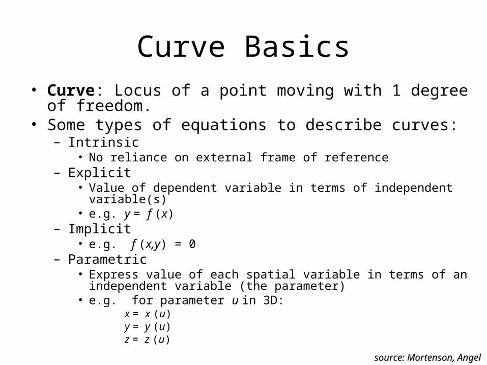
Curve Basics• Curve: Locus of a point moving with 1 degree of freedom.• Some types of equations to describe curves:
– Intrinsic• No reliance on external frame of reference
– Explicit• Value of dependent variable in terms of independent variable(s)• e.g. y = f (x)
– Implicit• e.g. f (x,y) = 0
– Parametric• Express value of each spatial variable in terms of an independent
variable (the parameter)• e.g. for parameter u in 3D:
x = x (u)y = y (u)z = z (u)
source: Mortenson, source: Mortenson, AngelAngel

Intrinsic Definition• No reliance on external frame of reference• Requires 2 equations as functions of arc
length* s:1) Curvature:
2) Torsion:
• For plane curves, alternatively:
)(1
sf
source: Mortensonsource: Mortenson
)(sg
*length measured along the curve
Torsion (in 3D) measures how much curve deviates from a plane curve.
Treated in more detail in Chapter 12 of Mortenson and Chapters 10, 19 of Farin.
ds
d
1

Explicit Form
• Value of dependent variable in terms of independent variable(s)– e.g. in 2D: one y value for each x value: y = f (x)– e.g. in 3D: y = f (x) and z = g (x)
• Axis-dependent• Not guaranteed to exist
– e.g. for 2D circle only one half is described by:
• Special cases can be problematic– e.g. y = mx + h is inappropriate for vertical lines
22 xry
source: Mortenson, source: Mortenson, AngelAngel

Implicit Form
• General form: f (x,y) = 0• Examples:
– Straight line: Ax + By + C=0 – Conic curve: Ax2 + 2Bxy + Cy2 + Dx + Ey + F=0
• Axis-dependent• Can represent all lines and circles and
more…• Some implicit forms are hard to
parameterize.
source: Mortenson, source: Mortenson, AngelAngel

Parametric Form
• Express value of each spatial variable in terms of an independent variable (the parameter)– e.g. for parameter u in 3D:
x = x (u)y = y (u)z = z (u)
• For a curve segment, typically • Curve segments can be joined to
form composite spline* (bendable) curves.
• Parametric form of a given curve is not necessarily unique.
• Every parametric form has an implicit form.
]1,0[u
source: Mortenson, source: Mortenson, AngelAngel
*see Mortenson p. 105 (or Farin p. 167) for spline definition as a “minimum energy curve.”
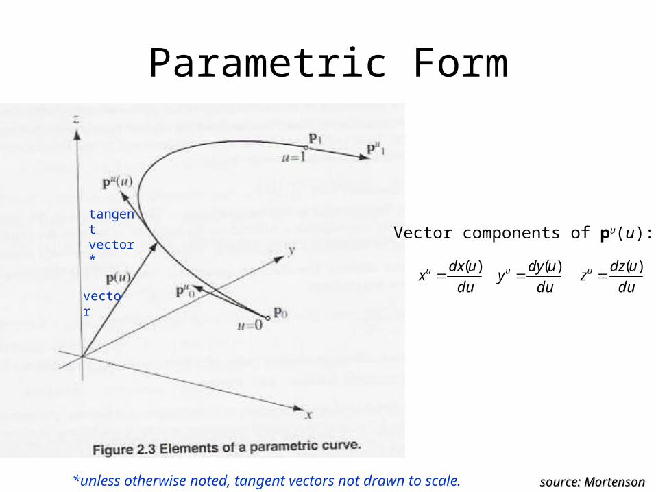
Parametric Form
source: Mortensonsource: Mortenson
vector
tangent vector*
*unless otherwise noted, tangent vectors not drawn to scale.
du
udzz
du
udyy
du
udxx uuu )(
)(
)(
Vector components of pu(u):

Parametric Form Advantages
• Allow separation of variables and direct computation of point coordinates.
• Accommodate all slopes.• Bounded when parameter lies in a
bounded interval.• More degrees of freedom to control curve
shape.• Various forms of continuity can be
enforced at curve segment join points.
source: Mortensonsource: MortensonSee Mortenson p.46 for more…
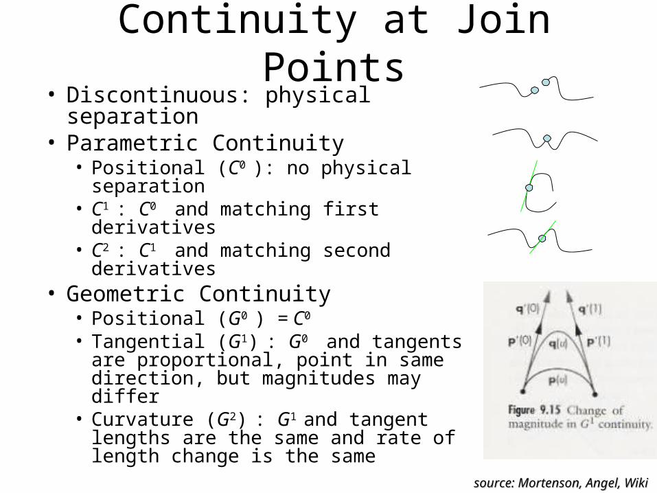
Continuity at Join Points• Discontinuous: physical separation• Parametric Continuity
• Positional (C0 ): no physical separation• C1 : C0 and matching first derivatives• C2 : C1 and matching second derivatives
• Geometric Continuity• Positional (G0 ) = C0
• Tangential (G1) : G0 and tangents are proportional, point in same direction, but magnitudes may differ
• Curvature (G2) : G1 and tangent lengths are the same and rate of length change is the same
source: Mortenson, Angel, source: Mortenson, Angel, WikiWiki

4 Typical Types of Parametric Curves
• Interpolating– Curve passes through all control points.
• Hermite– Defined by its 2 endpoints and tangent vectors at endpoints.– Interpolates all its control points.– Not invariant under affine transformations.– Special case of Bezier and B-Spline.
• Bezier– Interpolates first and last control points.– Curve is tangent to first and last segments of control polygon.– Easy to subdivide.– Curve segment lies within convex hull of control polygon.– Variation-diminishing.– Special case of B-spline.
• B-Spline– Not guaranteed to interpolate control points.– Invariant under affine transformations.– Curve segment lies within convex hull of control polygon.– Variation-diminishing.– Greater local control than Bezier.
Control points influence curve shape.
source: Mortenson, source: Mortenson, AngelAngel

Interpolating
• Interpolates all control points.• Geometric form:
• Rarely used due to lack of derivative continuity at curve segment join points.
source: Angelsource: Angel
n
iii ubu
0
)()( pp
cubic case with equally spaced parameter values

Hermite
• Geometric form (cubic case):
• Hermite curves can provide C1 continuity at curve segment join points.
234
233
232
231
)(
2)(
32)(
132)(
uuuF
uuuuF
uuuF
uuuF
source: Mortensonsource: Mortenson
14031201 )()()()()( uu uFuFuFuFu ppppp

Bezier• Geometric form (cubic case):
• Bezier curves can provide C1 continuity at curve segment join points.
n
iini uBu
0, )()( pp
source: Mortensonsource: Mortenson
inini uu
i
nuB
)1()(,
Bernstein polynomials.
n+1 = number of control points = degree + 1
Adding a control point elevates degree by 1.
Convex combination, so Bezier curve points all lie within convex hull of control polygon.
n
ini uB
0, 1)(
Rational form is invariant under perspective transformation:where hi are projective space coordinates (weights)
n
inii
n
iinii
uBh
uBhu
0,
0,
)(
)()(
pp

B-Spline
n
iiKi uNu
0, )()( pp
otherwise 0)(
if 1)(
1,
11,
uN
tutuN
i
iii
• Geometric form (non-uniform, non-rational case), where K controls degree (K -1) of basis functions:
• Cubic B-splines can provide C2 continuity at curve segment join points.
Convex combination, so B-spline curve points all lie within convex hull of control polygon.
n
iKi uN
0, 1)(
Rational form (NURBS) is invariant under perspective transformation, where hi are projective space coordinates (weights).
n
iKii
n
iiKii
uNh
uNhu
0,
0,
)(
)()(
pp
source: Mortensonsource: Mortenson
1
1,1
1
1,,
)()()()()(
iki
kiki
iki
kiiki tt
uNut
tt
uNtuuN
ti are knot values that relate u to the control points.
Uniform case: space knots at equal intervals of u.
Repeated knots move curve closer to control points.
N
N
N N
N
N N
N N

Geometric Modeling91.580.201
OpenGL Demoto accompany HW#2


