Geometric Optimization of Retroreflective Raised Pavement ...

University of South FloridaScholar Commons

Graduate Theses and Dissertations Graduate School

1-1-2013

Geometric Optimization of Retroreflective RaisedPavement MarkersLukai GuoUniversity of South Florida, [email protected]

Follow this and additional works at: http://scholarcommons.usf.edu/etd

Part of the Civil Engineering Commons

This Thesis is brought to you for free and open access by the Graduate School at Scholar Commons. It has been accepted for inclusion in GraduateTheses and Dissertations by an authorized administrator of Scholar Commons. For more information, please contact [email protected].

Scholar Commons CitationGuo, Lukai, "Geometric Optimization of Retroreflective Raised Pavement Markers" (2013). Graduate Theses and Dissertations.http://scholarcommons.usf.edu/etd/4498

http://scholarcommons.usf.edu/?utm_source=scholarcommons.usf.edu%2Fetd%2F4498&utm_medium=PDF&utm_campaign=PDFCoverPages

http://scholarcommons.usf.edu/?utm_source=scholarcommons.usf.edu%2Fetd%2F4498&utm_medium=PDF&utm_campaign=PDFCoverPages

http://scholarcommons.usf.edu?utm_source=scholarcommons.usf.edu%2Fetd%2F4498&utm_medium=PDF&utm_campaign=PDFCoverPages

http://scholarcommons.usf.edu/etd?utm_source=scholarcommons.usf.edu%2Fetd%2F4498&utm_medium=PDF&utm_campaign=PDFCoverPages

http://scholarcommons.usf.edu/grad?utm_source=scholarcommons.usf.edu%2Fetd%2F4498&utm_medium=PDF&utm_campaign=PDFCoverPages

http://scholarcommons.usf.edu/etd?utm_source=scholarcommons.usf.edu%2Fetd%2F4498&utm_medium=PDF&utm_campaign=PDFCoverPages

http://network.bepress.com/hgg/discipline/252?utm_source=scholarcommons.usf.edu%2Fetd%2F4498&utm_medium=PDF&utm_campaign=PDFCoverPages

mailto:[email protected]

Geometric Optimization of Retroreflective Raised Pavement Markers

by

Lukai Guo

A thesis submitted in partial fulfillment

of the requirements for the degree of

Master of Science in Civil Engineering

Department of Civil and Environmental Engineering

College of Engineering

University of South Florida

Major Professor: Qing Lu, Ph.D.

Abdul R. Pinjari, Ph.D.

Manjriker Gunaratne, Ph.D.

Date of Approval:

March 20, 2013

Keywords: Orthogonal Design, Regression Model,

Von Mises Stress, Survey, Finite Element

Copyright © 2013, Lukai Guo

DEDICATION

This thesis is dedicated to my father, Genlin Guo and my mother, Xiaoyan Lu for

their endless love, patience, and understanding. I am eternally indebted to them for their

generosity and encouragement through my life.

ACKNOWLEDGMENTS

Let me express my deepest gratitude to my advisor, Dr. Qing Lu, for his constant

guidance and support throughout my master program. I thank him for his active

encouragement, excellent inspiration and invaluable ideas that gave me the chance to

learn and experience research. I also would like to thank Dr. Pinjari and Dr. Gunaratne

for serving on my thesis committee. Special thanks to the teammate of my research group,

Bin Yu, who assisted me tremendously in completing the research and testing.

i

TABLE OF CONTENTS

LIST OF TABLES iii

LIST OF FIGURES v

ABSTRACT vii

CHAPTER 1: INTRODUCTION 1

1.1 Background 1

1.2 Organization of the Thesis 2

1.3 Types of RRPMs 2

1.3.1 With or Without Fill Materials 6

1.3.2 Squared Bottom or Bottom With Curves 6

CHAPTER 2: QUESTIONNAIRE SURVEY AND FIELD SURVEY 9

2.1 Details of Questionnaire Survey 9

2.2 Details of Field Survey 15

2.2.1 Site Selection 15

2.2.2 Field Survey in May, 2012 16

2.2.3 Field Survey in September, 2012 21

2.3 Summary of Current RRPM Conditions by Surveys 22

2.3.1 Questionnaire Survey 23

2.3.2 Field Survey 23

2.3.3 Manufacturers' Information 24

2.3.4 NTPEP Field Evaluation 24

2.3.5 Other Literature Review 25

CHAPTER 3: METHODOLOGY 27

3.1 Finite Element Model of Tire/Marker/Pavement Systems 27

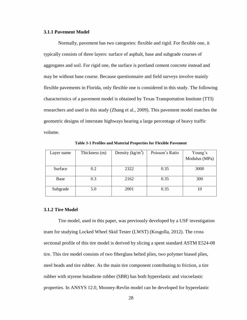
3.1.1 Pavement Model 28

3.1.2 Tire Model 28

3.1.3 RRPM Model 29

3.1.3.1 Details of RRPM Geometric Characteristics 29

3.1.3.2 Measurements of RRPMs and Material Properties 30

3.1.3.3 Building RRPM Models in ANSYS 32

3.1.4 Contact Model 33

3.1.5 Mesh Generation 34

3.1.6 Finite Element Model Assembly 35

3.2 Experimental Design 35

3.2.1 Orthogonal Design 36

ii

3.2.1.1 Basic Concept of Orthogonal Design 36

3.2.1.2 Four-level Fractional Factorial Design 39

3.2.2 Full Factorial Design 40

3.3 Stress Indicators Determination 41

3.3.1 Von Mises Stress 41

3.3.2 Principal Stress 42

3.3.3 Shear Stress on RRPM Bottom 42

3.3.4 Normal Stress on RRPM Bottom 43

CHAPTER 4: ANALYSIS OF SIMULATION RESULTS 44

4.1 Magnitudes and Distributions of Stresses on RRPMs 44

4.1.1 Von Mises Stress Magnitude and Distribution 44

4.1.2 Principal Stress Magnitude and Distribution 46

4.1.3 Shear Stress Magnitude and Distribution 47

4.1.4 Normal Stress Magnitude and Distribution 47

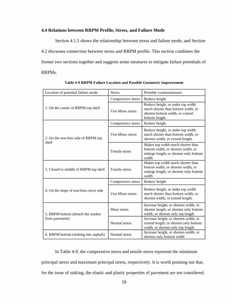
4.1.5 Relation between Stress and Failure Mode 48

4.2 Fractional Factorial Design Results 49

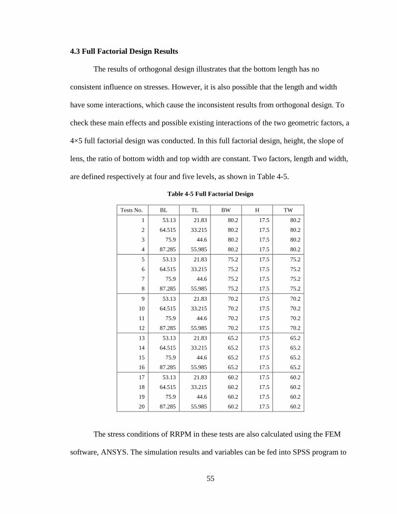
4.3 Full Factorial Design Results 55

4.3.1 Two-Factor Interaction Model 56

4.3.2 Simple Additive Model 57

4.4 Relations between RRPM Profile, Stress, and Failure Mode 59

4.5 Validation by Survey Results 60

CHAPTER 5: CONCLUSIONS AND FUTURE RESEARCH 62

5.1 Conclusions 62

5.2 Future Research 64

REFERENCES 65

iii

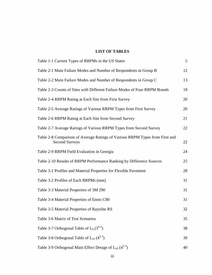
LIST OF TABLES

Table 1-1 Current Types of RRPMs in the US States 5

Table 2-1 Main Failure Modes and Number of Respondents in Group B 12

Table 2-2 Main Failure Modes and Number of Respondents in Group C 13

Table 2-3 Counts of Sites with Different Failure Modes of Four RRPM Brands 18

Table 2-4 RRPM Rating at Each Site from First Survey 20

Table 2-5 Average Ratings of Various RRPM Types from First Survey 20

Table 2-6 RRPM Rating at Each Site from Second Survey 21

Table 2-7 Average Ratings of Various RRPM Types from Second Survey 22

Table 2-8 Comparison of Average Ratings of Various RRPM Types from First and

Second Surveys 22

Table 2-9 RRPM Field Evaluation in Georgia 24

Table 2-10 Results of RRPM Performance Ranking by Difference Sources 25

Table 3-1 Profiles and Material Properties for Flexible Pavement 28

Table 3-2 Profiles of Each RRPMs (mm) 31

Table 3-3 Material Properties of 3M 290 31

Table 3-4 Material Properties of Ennis C80 31

Table 3-5 Material Properties of Rayolite RS 32

Table 3-6 Matrix of Test Scenarios 35

Table 3-7 Orthogonal Table of L9 (34-2

) 38


) 39

Table 3-9 Orthogonal Main Effect Design of L16 (45-3

) 40

iv

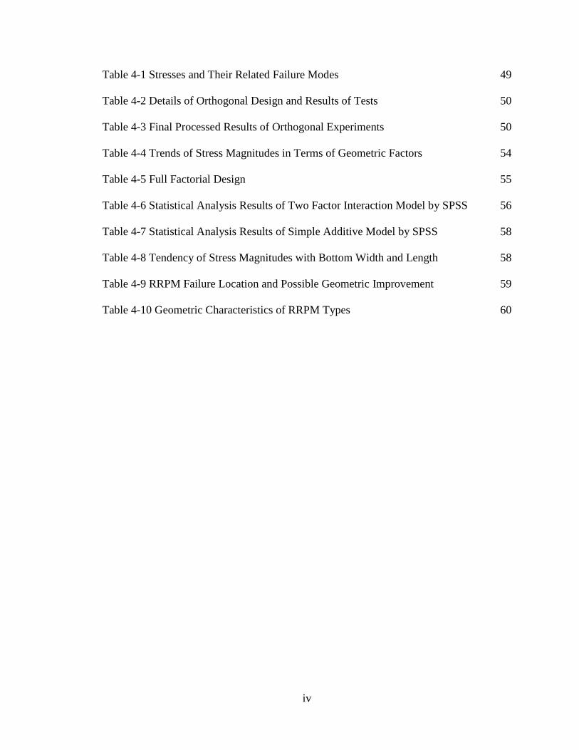
Table 4-1 Stresses and Their Related Failure Modes 49

Table 4-2 Details of Orthogonal Design and Results of Tests 50

Table 4-3 Final Processed Results of Orthogonal Experiments 50

Table 4-4 Trends of Stress Magnitudes in Terms of Geometric Factors 54

Table 4-5 Full Factorial Design 55

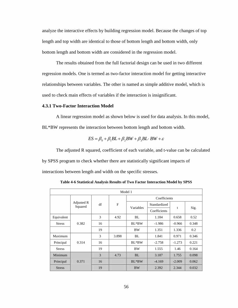
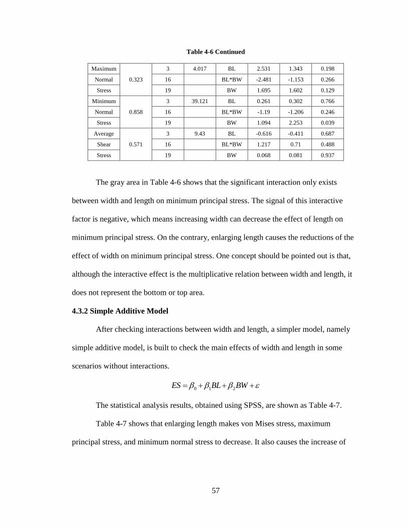
Table 4-6 Statistical Analysis Results of Two Factor Interaction Model by SPSS 56

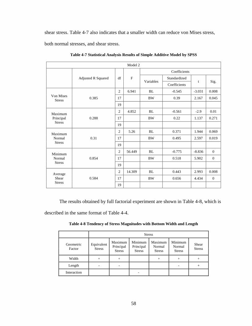
Table 4-7 Statistical Analysis Results of Simple Additive Model by SPSS 58

Table 4-8 Tendency of Stress Magnitudes with Bottom Width and Length 58

Table 4-9 RRPM Failure Location and Possible Geometric Improvement 59

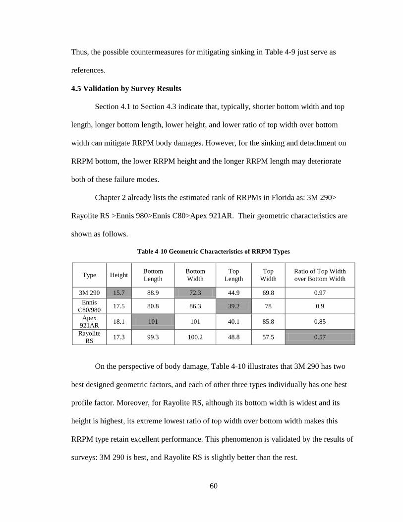
Table 4-10 Geometric Characteristics of RRPM Types 60

v

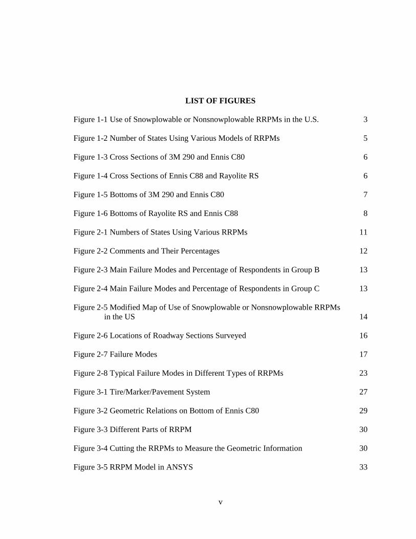
LIST OF FIGURES

Figure 1-1 Use of Snowplowable or Nonsnowplowable RRPMs in the U.S. 3

Figure 1-2 Number of States Using Various Models of RRPMs 5

Figure 1-3 Cross Sections of 3M 290 and Ennis C80 6

Figure 1-4 Cross Sections of Ennis C88 and Rayolite RS 6

Figure 1-5 Bottoms of 3M 290 and Ennis C80 7

Figure 1-6 Bottoms of Rayolite RS and Ennis C88 8

Figure 2-1 Numbers of States Using Various RRPMs 11

Figure 2-2 Comments and Their Percentages 12

Figure 2-3 Main Failure Modes and Percentage of Respondents in Group B 13

Figure 2-4 Main Failure Modes and Percentage of Respondents in Group C 13

Figure 2-5 Modified Map of Use of Snowplowable or Nonsnowplowable RRPMs

in the US 14

Figure 2-6 Locations of Roadway Sections Surveyed 16

Figure 2-7 Failure Modes 17

Figure 2-8 Typical Failure Modes in Different Types of RRPMs 23

Figure 3-1 Tire/Marker/Pavement System 27

Figure 3-2 Geometric Relations on Bottom of Ennis C80 29

Figure 3-3 Different Parts of RRPM 30

Figure 3-4 Cutting the RRPMs to Measure the Geometric Information 30

Figure 3-5 RRPM Model in ANSYS 33

vi

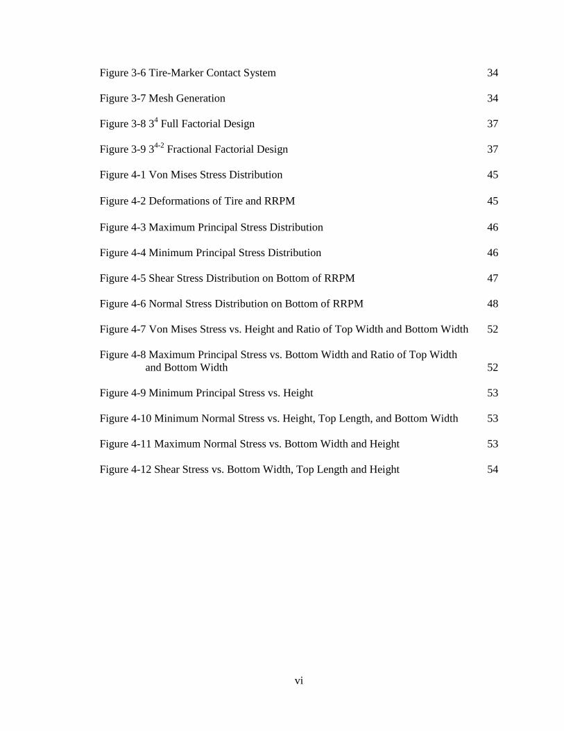
Figure 3-6 Tire-Marker Contact System 34

Figure 3-7 Mesh Generation 34

Figure 3-8 34 Full Factorial Design 37

Figure 3-9 34-2

Fractional Factorial Design 37

Figure 4-1 Von Mises Stress Distribution 45

Figure 4-2 Deformations of Tire and RRPM 45

Figure 4-3 Maximum Principal Stress Distribution 46

Figure 4-4 Minimum Principal Stress Distribution 46

Figure 4-5 Shear Stress Distribution on Bottom of RRPM 47

Figure 4-6 Normal Stress Distribution on Bottom of RRPM 48

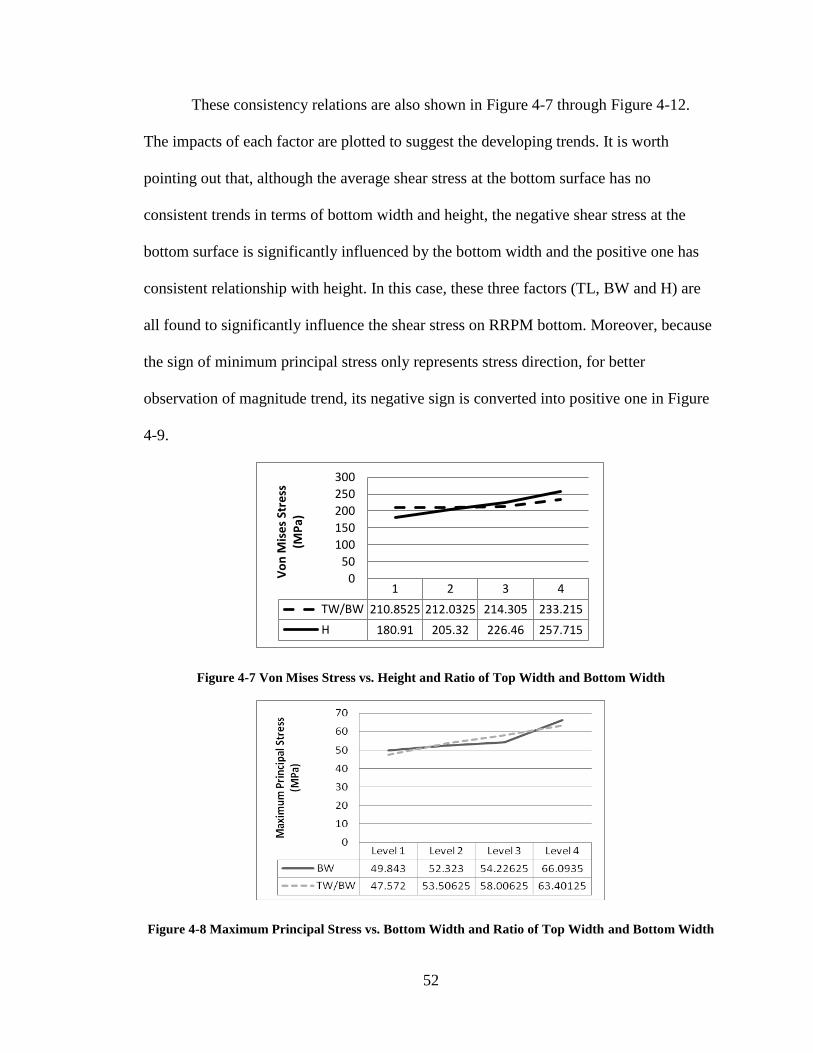
Figure 4-7 Von Mises Stress vs. Height and Ratio of Top Width and Bottom Width 52

Figure 4-8 Maximum Principal Stress vs. Bottom Width and Ratio of Top Width

and Bottom Width 52

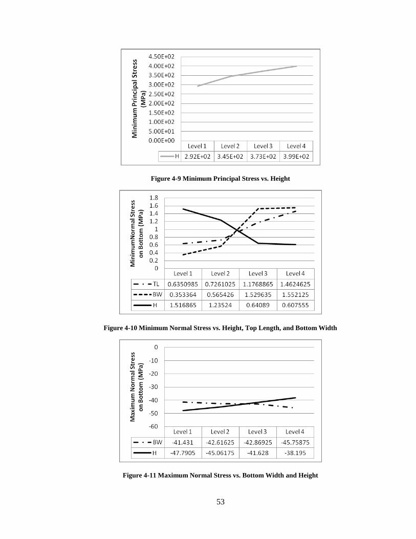
Figure 4-9 Minimum Principal Stress vs. Height 53

Figure 4-10 Minimum Normal Stress vs. Height, Top Length, and Bottom Width 53

Figure 4-11 Maximum Normal Stress vs. Bottom Width and Height 53

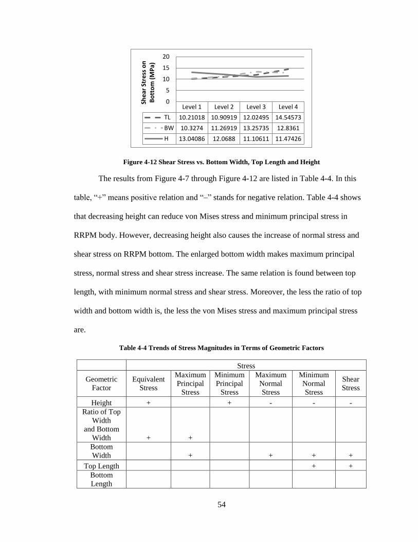
Figure 4-12 Shear Stress vs. Bottom Width, Top Length and Height 54

vii

ABSTRACT

As the field service life of retroreflective raised pavement marker (RRPM) is

much shorter than expected, it is necessary to identify the causes and thus improve the

RRPM structural design to mitigate the main failure modes, such as poor retention from

pavements, structural damage, and loss of retroreflectivity. One strategy for extending

RRPM service life is to enhance RRPM geometric characteristics to decrease critical

stresses in markers. The main purpose of this thesis is to analyze the relationship between

stresses, failure modes, and RRPM profiles. Based on this research, some measures are

suggested in order to avoid corresponding failure modes by optimizing RRPM profiles.

The information about current performance of different types of RRPMs is

summarized through literature review, questionnaire surveys, and a series of field surveys

in Tampa bay area. Field survey observations show that the RRPM failure modes include

lens cracking, lens loss, body cracking, body breakage, complete loss of RRPMs from

pavement surface, severe abrasion or contamination of the retroreflective faces, and

sinking of RRPMs into asphalt concrete. The overall performances of RRPMs in

surveyed pavement sections are summarized and ranked as: 3M 290> Rayolite

RS >Ennis 980>Ennis C80>Apex 921AR.

The distributions and magnitudes of various stress indicators, such as von Mises

stress, principal stress, shear stress and normal stress within the RRPM structure, are

estimated by finite element model (FEM) of pavement/tire/marker systems in ANSYS

viii

software. Based on finite element model simulations, the critical stresses in the RRPMs

and the observed failure modes are linked. Both the critical von Mises stress and

compressive stress are concentrated on the rims and corners of the markers’ top surface.

Tensile stress is produced on the mid-top of markers’ shell and distributed symmetrically.

For shear stress at the RRPM bottom, the maximum one occurs on the non-lens sides of

the RRPM. Upward normal stress, which may cause RRPM detachment from pavement,

exists at the bottom, especially on the edge of lens side and at the middle of the curve

edge.

One orthogonal experiment of a matrix of L16 (45-3

) and one full factorial

experiment of 4×5 were used to guide the FME simulations. Based on the stress

magnitudes variations on different RRPM types, the relationships between the RRPM

profiles and the stresses are obtained. It is found that RRPMs of geometric designs of

smaller bottom width and top length, larger bottom length, lower height, and lower ratio

of top width over bottom width witness decreases of experienced critical stresses.

1

CHAPTER 1: INTRODUCTION

1.1 Background

Retroreflective raised pavement marker (RRPM) is a device that is applied as a

positioning guide to supplement or substitute for pavement markings (FHWA, 2003),

especially during night and wet weather conditions when the pavement markings

experience a substantial reduction of retroreflectivity. Moreover, RRPM can also cause

vehicle vibration and audible tone to alert drivers for crossing over it (NCHRP, 2004).

However, the Texas Department of Transportation conducted a number of studies

to conclude that most RRPMs lose reflectivity over very short periods of time (Hofmann

and Dunning, 1995). In recent years, RRPMs exhibited poor field performance, such as

poor retention on pavements, structural damage, and loss of retroreflectivity (Zhang et al.,

2009).

These unexpected damages significantly reduce RRPM service life. Considering

the relatively high cost of RRPM (material and installation), based on benefit-cost

calculation, most states do not install RRPMs if pavement overlay or replacement is

scheduled within five years or less (Matthias, 1988; Zador et al., 1982). This strategy also

can be interpreted that the anticipated RRPM service life should be beyond five years,

otherwise the negative profit appears. However, questionnaire survey, conducted by a

University of South Florida (USF) investigation team, shows that the average RRPM

2

service life is 28.6 months, which is less than half of the expected minimum service life.

Therefore, it is important to investigate how to extend the RRPM service life.

1.2 Organization of the Thesis

The thesis is organized as follows. As a preparation for the study, the remainder

of Chapter 1 introduces all types of RRPMs, which were collected by searching all states

Department of Transportation (DOT) specifications and attached Qualified Product Lists

(QPLs). Chapter 2 shows the current performance of these RRPMs according to

questionnaire and field surveys. The questionnaire survey was conducted with

participants including maintenance engineers, contract managers, and other personnel in

various state DOTs. The field surveys were conducted around the Tampa Bay area of

Florida. Chapter 3 describes the methodology of building a finite element model (FEM)

of the tire/marker/pavement system to simulate the RRPM conditions in the real world.

Chapter 3 also describes the experimental designs, including one orthogonal design and

one full factorial design. The rest of Chapter 3 introduces different critical stresses and

why these types of stresses are considered. Chapter 4 is divided into three parts. The first

part analyzes the magnitudes and locations of critical stresses on some typical size

RRPMs. The second part conducts statistical analysis of stresses. The third part verifies

the FEM simulation results based on the survey results in Chapter 2. Conclusions and

future researches are listed in Chapter 5.

1.3 Types of RRPMs

RRPMs can be classified in various ways based on their structures and functions.

According to a common classification used in Florida Department of Transportation

(FDOT) 2010 Standard Specifications for Road and Bridge Construction, Section 970,

3

RRPMs in Florida are mainly grouped into four classes: Class A for temporary, Class B

for permanent, Class D for work zone, and Class E for temporary work zone. Many other

states further separate the permanent RRPMs into two subcategories: snowplowable and

nonsnowplowable. Snowplowable RRPMs typically consist of cast iron housing and

reflective lens, and are used in snowplow regions, like the northern states of the USA.

Nonsnowplowable RRPMs do not have protective housing, and thus are only suited for

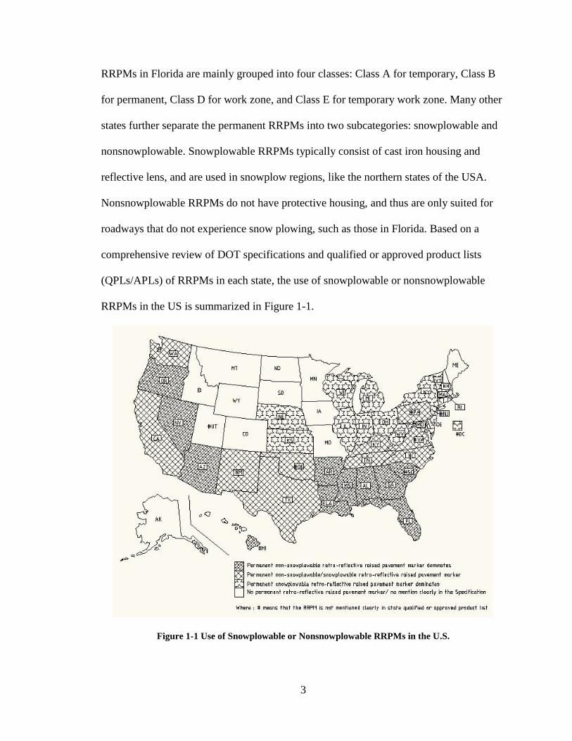
roadways that do not experience snow plowing, such as those in Florida. Based on a

comprehensive review of DOT specifications and qualified or approved product lists

(QPLs/APLs) of RRPMs in each state, the use of snowplowable or nonsnowplowable

RRPMs in the US is summarized in Figure 1-1.

Figure 1-1 Use of Snowplowable or Nonsnowplowable RRPMs in the U.S.

4

Figure 1-1 shows that the states using permanent nonsnowplowable RRPMs are

concentrated in the southern areas where air temperature is relatively high. This map also

shows that, in many northern areas, permanent nonsnowplowable RRPMs are typically

not installed.

Since this study is intended for the RRPM use in Florida of rare snow chances,

only nonsnowplowable RRPMs are of interests. Figure 1-1 shows how widely this type of

RRPMs is used. Because all information in this map was derived from DOT

specifications and QPLs/APLs, the map only describes the current use of RRPMs on U.S.

Route highways, U.S. Interstate highways, and State Route highways. The use of RRPMs

on local roads and streets is not included. During the survey, it was discovered that a few

states have recently stopped the use of nonsnowplowable RRPMs and begun to use

snowplowable ones instead.

Based on the state DOT QPLs/APLs, four companies are mainly approved for

providing nonsnowplowable RRPMs:

1) 3M

2) Ennis/Stimsonite

3) Ray-o-lite, and

4) Apex

For 3M, the major product is 290 series, including 290PSA series (PSA stands for

pressure sensitive adhesive, which means a simple pressure can activate the adhesive

function); For Ennis/Stimsonite, the company provides 6 widely used types of RRPMs:

C80, C88, Model 911, Model 980, Model 948, and Model 953; For Apex, only 921AR is

mentioned, but widely appearing, on the States QPL/APL; For Ray-o-lite, the AA (All

5

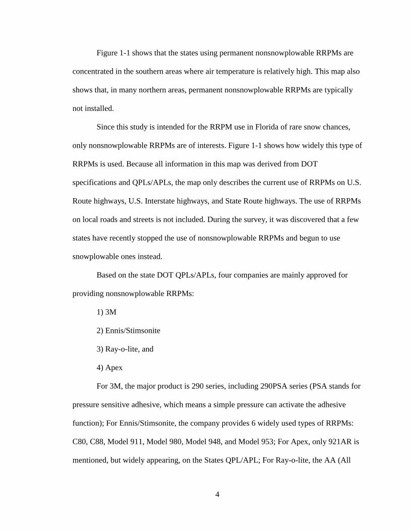
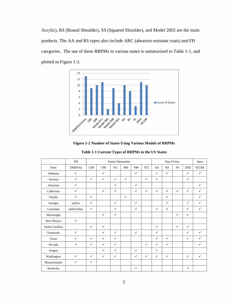
Acrylic), RS (Round Shoulder), SS (Squared Shoulder), and Model 2002 are the main

products. The AA and RS types also include ARC (abrasion resistant coats) and FH

categories. The use of these RRPMs in various states is summarized in Table 1-1, and

plotted in Figure 1-2.

Figure 1-2 Number of States Using Various Models of RRPMs

Table 1-1 Current Types of RRPMs in the US States

3M Ennis/ Stimsonite Ray-O-Lite Apex

State 290(PSA) C80 C88 911 980 948 953 AA RS SS 2002 921AR

Alabama

Arizona

Arkansas

California

Florida

Georgia yellow

Louisiana yellow/blue

Mississippi

New Mexico

North Carolina

Tennessee

Texas

Nevada

Oregon

Washington

Massachusetts

Kentucky

6

According to their various materials and structures, RRPMs can be grouped as

follows.

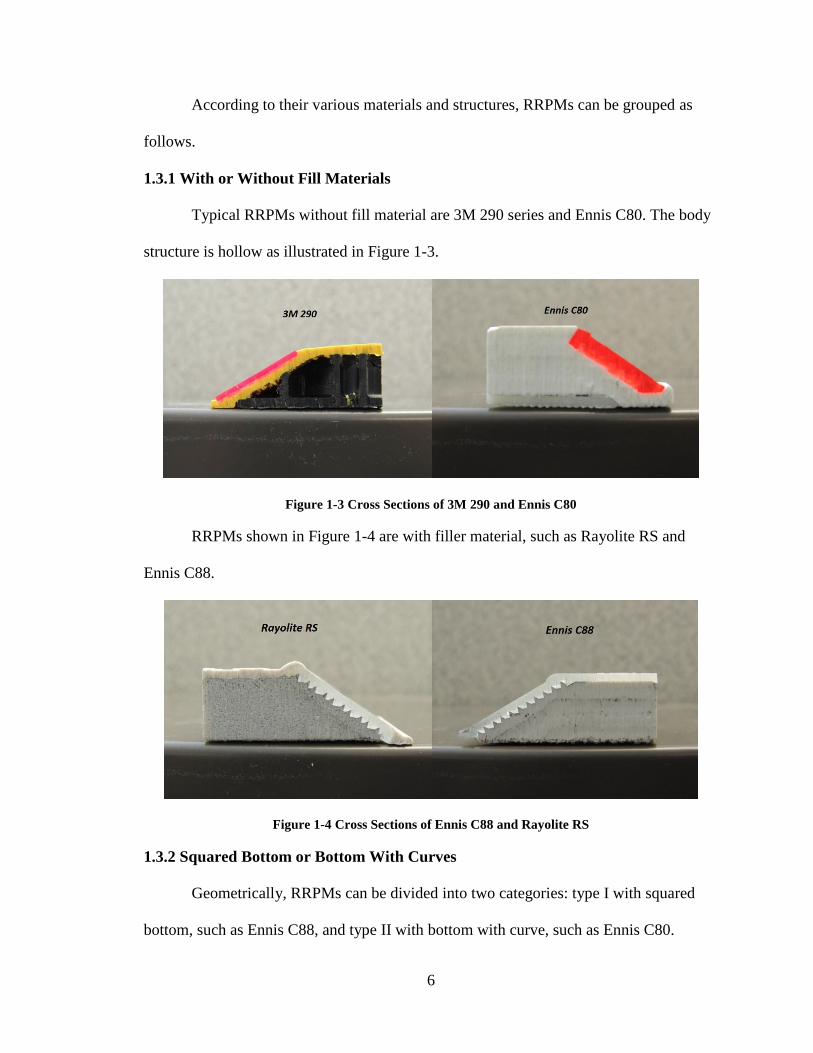
1.3.1 With or Without Fill Materials

Typical RRPMs without fill material are 3M 290 series and Ennis C80. The body

structure is hollow as illustrated in Figure 1-3.

Figure 1-3 Cross Sections of 3M 290 and Ennis C80

RRPMs shown in Figure 1-4 are with filler material, such as Rayolite RS and

Ennis C88.

Figure 1-4 Cross Sections of Ennis C88 and Rayolite RS

1.3.2 Squared Bottom or Bottom With Curves

Geometrically, RRPMs can be divided into two categories: type I with squared

bottom, such as Ennis C88, and type II with bottom with curve, such as Ennis C80.

7

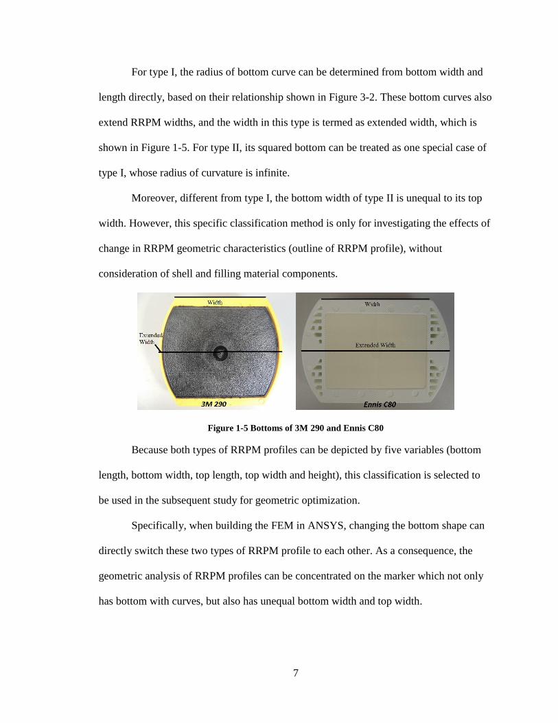
For type I, the radius of bottom curve can be determined from bottom width and

length directly, based on their relationship shown in Figure 3-2. These bottom curves also

extend RRPM widths, and the width in this type is termed as extended width, which is

shown in Figure 1-5. For type II, its squared bottom can be treated as one special case of

type I, whose radius of curvature is infinite.

Moreover, different from type I, the bottom width of type II is unequal to its top

width. However, this specific classification method is only for investigating the effects of

change in RRPM geometric characteristics (outline of RRPM profile), without

consideration of shell and filling material components.

Figure 1-5 Bottoms of 3M 290 and Ennis C80

Because both types of RRPM profiles can be depicted by five variables (bottom

length, bottom width, top length, top width and height), this classification is selected to

be used in the subsequent study for geometric optimization.

Specifically, when building the FEM in ANSYS, changing the bottom shape can

directly switch these two types of RRPM profile to each other. As a consequence, the

geometric analysis of RRPM profiles can be concentrated on the marker which not only

has bottom with curves, but also has unequal bottom width and top width.

8

Figure 1-6 Bottoms of Rayolite RS and Ennis C88

9

CHAPTER 2: QUESTIONNAIRE SURVEY AND FIELD SURVEY

2.1 Details of Questionnaire Survey

To collect up-to-date information on RRPMs from experienced engineers and

specialists, a questionnaire survey was developed and distributed electronically across the

nation. The respondents include maintenance engineers, contract managers, and other

personnel in various state DOTs. Based on the relevancy to the purposes of the study, the

respondents are divided into three groups: Group A from FDOT District 7 (Tampa area),

Group B from other FDOT Districts, and Group C from other states (mainly DOT

personnel with a few from the industry). The questions in the questionnaire vary slightly

among the three groups. Among a total of 11 questions in the questionnaire survey, only

two are directly related to geometric optimization. In this study, these two questions and

corresponding responses are summarized, as follows, to provide useful information for

further analysis.

Question 1 to Groups A, B, and C is what types of RRPMs (based on FDOT

qualified product list if in Florida) are most commonly used? Why? Are there any

RRPMs seen as good markers and any seen as bad markers in terms of field performance?

Response from Group A shows that 3M and Stimsonite are more commonly used

due to pricing. 3M is seen as a good marker which has a longer life on the road and

Stimsonite as not so good in the area of field performance. The markers shall comply

10

with ASTM D 4280 Class A (no abrasion treatment) and Class B (with abrasion

treatment).

Response from Group B shows that Type B markers which are listed on the

FDOT QPL are only used. The certification of materials is checked before beginning

work. No significant difference in performance between manufacturers.

Response from Group C shows that Georgia uses 2×4 inches or 4×4 inches size

RRPMs. All approved markers have similar service lives. In South Carolina, plastic

makers with reflective surfaces, such as the 3M markers, have become more popular in

recent years. Typically, Ray-O-Lite, Ennis (Stimsonite) and 3M markers which meet the

general requirements of specifications are used on contracts. Louisiana uses 3M because

of low bids. Contractors also seem to use more of the Ennis and Ray-O-lite markers. The

Ennis markers seem to hold up better.

Arkansas uses 3M, Ennis, and Ray-O-Lite markers according to Supply Contract

Specifications. No significant difference exists in performance between manufacturers. In

Arizona, 3M 290 markers have dominated for quite a while. Ennis 88, 911 and 980, Apex

920 or 921, Ray-O-Lite round shoulder, ARC II markers have been approved, but are not

often used. Washington State typically uses the Stimsonite model 88 RRPMs in Olympic

Region because they last up to the plow abuse and normal highway use. Other RRPMs

similar to the Stimsonite 948 ones are also used in Washington but they do not hold up

well.

One respondent from California thinks that 3M is the best type: they seem to

outlast all others by far as reflectivity is concerned. Respondents from Nevada and North

Carolina only mentioned 3M but no significant difference exists.

11

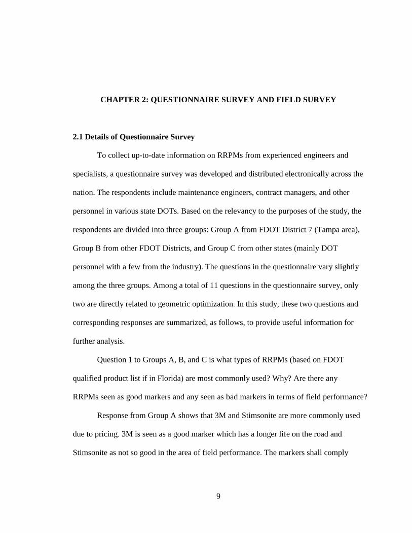
Thus, 3M, Ennis, and Ray-O-Lite are the most popular RRPMs manufacturers in

these states. 3M has dominated for quite a while because of its low bids and good

performance. Apparently, the types of applied RRPMs vary with states, but the

mainstream exists. Figure 2-1 shows that all these 7 states use 3M, and adversely, Apex is

not so popular.

For field performance, Group A prefers 3M, and regards Stimsonite as not so

good. Group B claims that there is no significant difference in performance between

manufacturers.

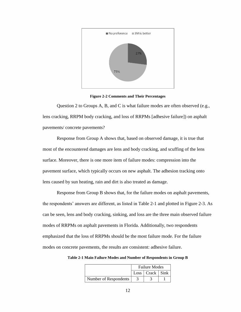
In Group C, three respondents have the same comment as Group B. One

respondent from Louisiana feels that Ennis seems to hold up better, and another

respondent from Arizona replies that 3M dominates. Figure 2-2 shows that most of the

respondents feel no significant difference in field performance of these approved RRPMs.

Figure 2-1 Numbers of States Using Various RRPMs

0

2

4

6

8

10

12

3M Ray-O-Lite Ennis Apex

12

Figure 2-2 Comments and Their Percentages

Question 2 to Groups A, B, and C is what failure modes are often observed (e.g.,

lens cracking, RRPM body cracking, and loss of RRPMs [adhesive failure]) on asphalt

pavements/ concrete pavements?

Response from Group A shows that, based on observed damage, it is true that

most of the encountered damages are lens and body cracking, and scuffing of the lens

surface. Moreover, there is one more item of failure modes: compression into the

pavement surface, which typically occurs on new asphalt. The adhesion tracking onto

lens caused by sun heating, rain and dirt is also treated as damage.

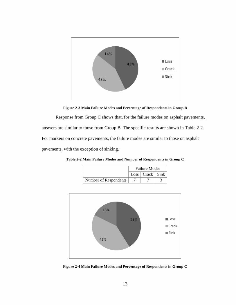
Response from Group B shows that, for the failure modes on asphalt pavements,

the respondents’ answers are different, as listed in Table 2-1 and plotted in Figure 2-3. As

can be seen, lens and body cracking, sinking, and loss are the three main observed failure

modes of RRPMs on asphalt pavements in Florida. Additionally, two respondents

emphasized that the loss of RRPMs should be the most failure mode. For the failure

modes on concrete pavements, the results are consistent: adhesive failure.

Table 2-1 Main Failure Modes and Number of Respondents in Group B

Failure Modes

Loss Crack Sink

Number of Respondents 3 3 1

13

Figure 2-3 Main Failure Modes and Percentage of Respondents in Group B

Response from Group C shows that, for the failure modes on asphalt pavements,

answers are similar to those from Group B. The specific results are shown in Table 2-2.

For markers on concrete pavements, the failure modes are similar to those on asphalt

pavements, with the exception of sinking.

Table 2-2 Main Failure Modes and Number of Respondents in Group C

Failure Modes

Loss Crack Sink

Number of Respondents 7 7 3

Figure 2-4 Main Failure Modes and Percentage of Respondents in Group C

14

Thus, based on the respondents’ answers, it is safe to say that lens and body crack

and loss of RRPMs are the main failure modes, and their proportions are almost equal.

This questionnaire survey also asked respondents for some suggestion, which can

be done, to extend RRPM service life. There are two suggestions related to optimizing

RRPM geometric characteristics. One is to decrease the RRPM profile height, and the

other is to enlarge RRPM bottom area. These suggestions will be checked in Chapter 4.

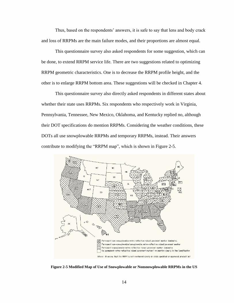
This questionnaire survey also directly asked respondents in different states about

whether their state uses RRPMs. Six respondents who respectively work in Virginia,

Pennsylvania, Tennessee, New Mexico, Oklahoma, and Kentucky replied no, although

their DOT specifications do mention RRPMs. Considering the weather conditions, these

DOTs all use snowplowable RRPMs and temporary RRPMs, instead. Their answers

contribute to modifying the “RRPM map”, which is shown in Figure 2-5.

Figure 2-5 Modified Map of Use of Snowplowable or Nonsnowplowable RRPMs in the US

15

2.2 Details of Field Survey

In the summer and the fall of 2012, two field surveys with several objectives were

conducted to record the conditions of RRPMs installed on selected FDOT roadways.

Considering optimization of RRPM geometric characteristics, only the following two

parts are discussed in this study:

1) Which types of RRPMs are widely used on FDOT roadways and how do they

perform?

2) Which major failure modes do the RRPMs exhibit in the field?

2.2.1 Site Selection

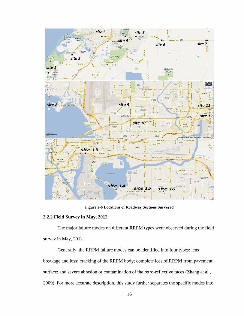
The roadway sections surveyed, as shown in Figure 2-6, were selected through

consulting with FDOT personnel to cover various marker types and damage conditions

and high and low traffic volumes. One route, starting 10 miles south of Ruskin, along US

41, and then turning to SR 674, till the intersection with Plant City-Picnic Rd. The second

route is along the Dale Mabry Hwy and 22 St, which are connected by SR 60. The third

route is along 22 St, crossing SR 60, to the Causeway Blvd, until the intersection with

Maydell Dr. These sections have various geometric features, such as tangent, horizontal

curve, vertical curve, width and position (entry and departure approaches at intersections).

The current traffic conditions, such as annual average daily traffic (AADT), truck volume,

pavement surface condition (e.g., cracking and roughness) are also different.

The geometric characteristics and the conditions of the roadways were determined

from the geographic information system (GIS) data and Straight Line Diagrams (SLDs),

which are both available on FDOT website. The RRPMs and their failure modes were

recorded by a digital camera.

16

Figure 2-6 Locations of Roadway Sections Surveyed

2.2.2 Field Survey in May, 2012

The major failure modes on different RRPM types were observed during the field

survey in May, 2012.

Generally, the RRPM failure modes can be identified into four types: lens

breakage and loss; cracking of the RRPM body; complete loss of RRPM from pavement

surface; and severe abrasion or contamination of the retro-reflective faces (Zhang et al.,

2009). For more accurate description, this study further separates the specific modes into

17

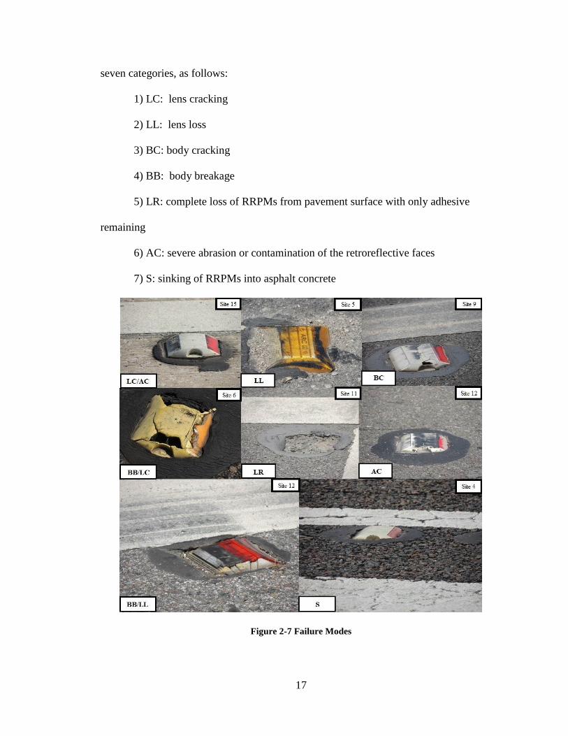
seven categories, as follows:

1) LC: lens cracking

2) LL: lens loss

3) BC: body cracking

4) BB: body breakage

5) LR: complete loss of RRPMs from pavement surface with only adhesive

remaining

6) AC: severe abrasion or contamination of the retroreflective faces

7) S: sinking of RRPMs into asphalt concrete

Figure 2-7 Failure Modes

18

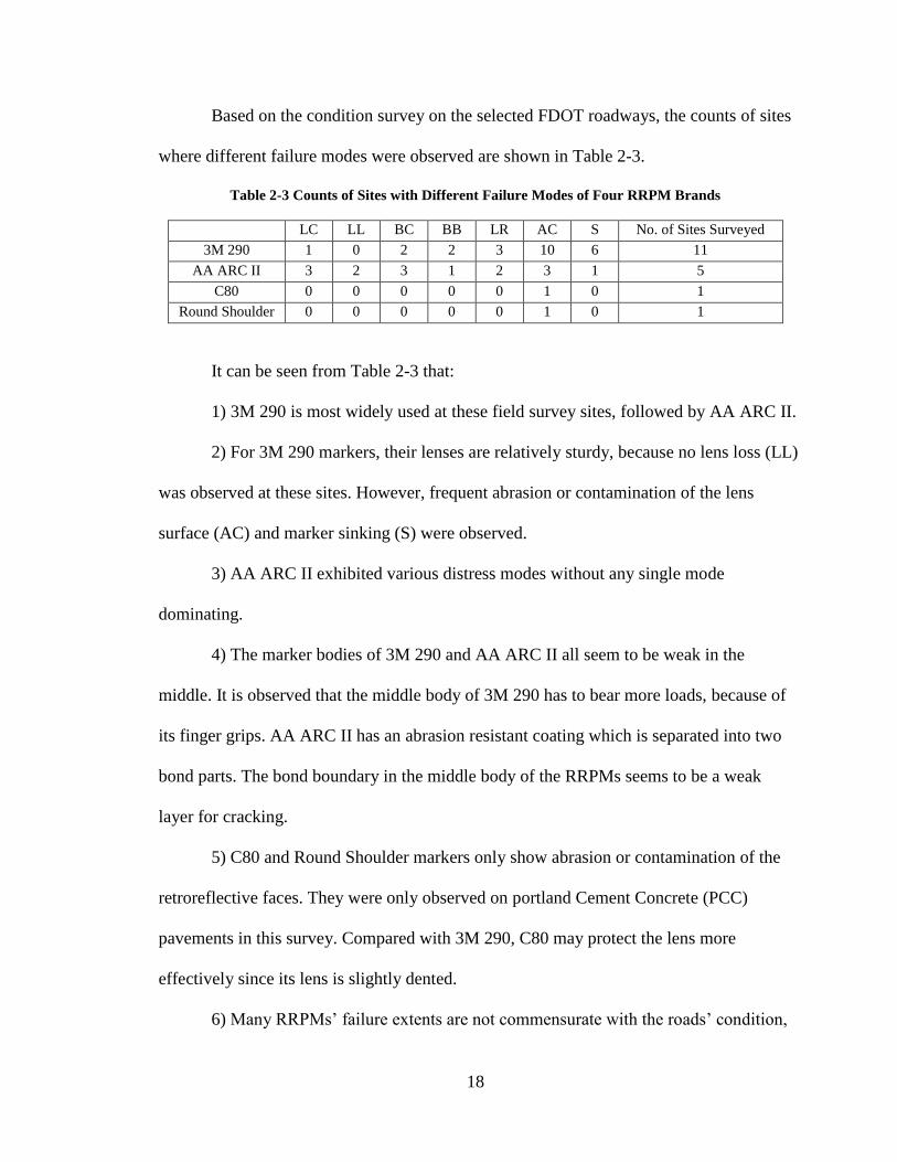
Based on the condition survey on the selected FDOT roadways, the counts of sites

where different failure modes were observed are shown in Table 2-3.

Table 2-3 Counts of Sites with Different Failure Modes of Four RRPM Brands

LC LL BC BB LR AC S No. of Sites Surveyed

3M 290 1 0 2 2 3 10 6 11

AA ARC II 3 2 3 1 2 3 1 5

C80 0 0 0 0 0 1 0 1

Round Shoulder 0 0 0 0 0 1 0 1

It can be seen from Table 2-3 that:

1) 3M 290 is most widely used at these field survey sites, followed by AA ARC II.

2) For 3M 290 markers, their lenses are relatively sturdy, because no lens loss (LL)

was observed at these sites. However, frequent abrasion or contamination of the lens

surface (AC) and marker sinking (S) were observed.

3) AA ARC II exhibited various distress modes without any single mode

dominating.

4) The marker bodies of 3M 290 and AA ARC II all seem to be weak in the

middle. It is observed that the middle body of 3M 290 has to bear more loads, because of

its finger grips. AA ARC II has an abrasion resistant coating which is separated into two

bond parts. The bond boundary in the middle body of the RRPMs seems to be a weak

layer for cracking.

5) C80 and Round Shoulder markers only show abrasion or contamination of the

retroreflective faces. They were only observed on portland Cement Concrete (PCC)

pavements in this survey. Compared with 3M 290, C80 may protect the lens more

effectively since its lens is slightly dented.

6) Many RRPMs’ failure extents are not commensurate with the roads’ condition,

19

such as those at sites 1, 2, 4, 5, 8, 9, 10, 13, 14, and 15. These sites sustained heavy truck

traffic and showed pavement distresses such as cracking, but the markers looked fine.

One potential reason is that the markers had been replaced frequently. One example is at

site 13 (on SR 60), where the remaining adhesives on the pavement indicated that the

markers had been replaced for at least four times in the last few years. The age

information of the markers, however, could not be obtained from FDOT, which limited

the extent of analysis of the field data and made ensuing field surveys indispensable.

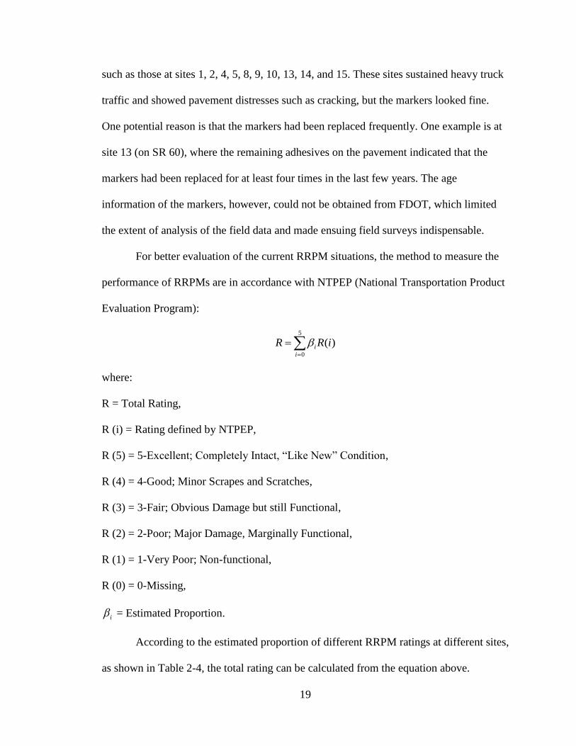
For better evaluation of the current RRPM situations, the method to measure the

performance of RRPMs are in accordance with NTPEP (National Transportation Product

Evaluation Program):

5

0

( )i

i

R R i

where:

R = Total Rating,

R (i) = Rating defined by NTPEP,

R (5) = 5-Excellent; Completely Intact, “Like New” Condition,

R (4) = 4-Good; Minor Scrapes and Scratches,

R (3) = 3-Fair; Obvious Damage but still Functional,

R (2) = 2-Poor; Major Damage, Marginally Functional,

R (1) = 1-Very Poor; Non-functional,

R (0) = 0-Missing,

i = Estimated Proportion.

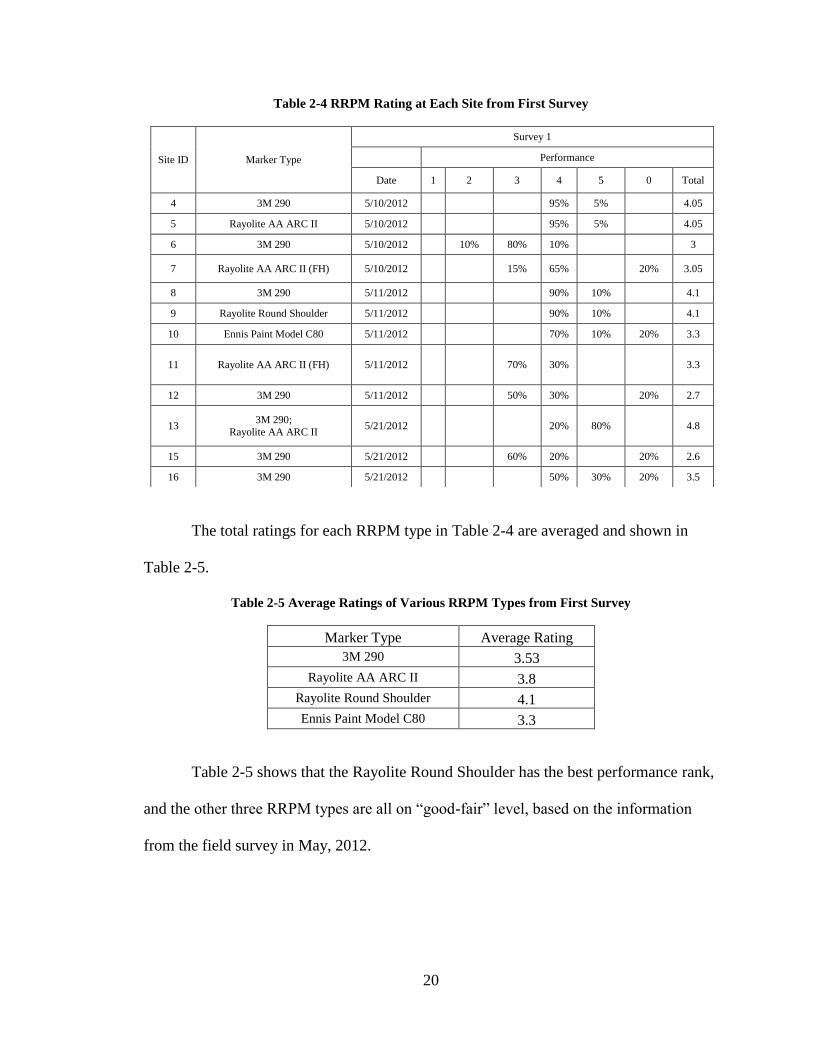
According to the estimated proportion of different RRPM ratings at different sites,

as shown in Table 2-4, the total rating can be calculated from the equation above.

20

Table 2-4 RRPM Rating at Each Site from First Survey

The total ratings for each RRPM type in Table 2-4 are averaged and shown in

Table 2-5.

Table 2-5 Average Ratings of Various RRPM Types from First Survey

Marker Type Average Rating

3M 290 3.53

Rayolite AA ARC II 3.8

Rayolite Round Shoulder 4.1

Ennis Paint Model C80 3.3

Table 2-5 shows that the Rayolite Round Shoulder has the best performance rank,

and the other three RRPM types are all on “good-fair” level, based on the information

from the field survey in May, 2012.

Site ID Marker Type

Survey 1

Performance

Date 1 2 3 4 5 0 Total

4 3M 290 5/10/2012 95% 5% 4.05

5 Rayolite AA ARC II 5/10/2012 95% 5% 4.05

6 3M 290 5/10/2012 10% 80% 10% 3

7 Rayolite AA ARC II (FH) 5/10/2012 15% 65% 20% 3.05

8 3M 290 5/11/2012 90% 10% 4.1

9 Rayolite Round Shoulder 5/11/2012 90% 10% 4.1

10 Ennis Paint Model C80 5/11/2012 70% 10% 20% 3.3

11 Rayolite AA ARC II (FH) 5/11/2012 70% 30% 3.3

12 3M 290 5/11/2012 50% 30% 20% 2.7

13 3M 290;

Rayolite AA ARC II 5/21/2012 20% 80% 4.8

15 3M 290 5/21/2012 60% 20% 20% 2.6

16 3M 290 5/21/2012 50% 30% 20% 3.5

21

2.2.3 Field Survey in September, 2012

To clear the confounding effect of various RRPM ages, one ensuing field

evaluation after four months was made to check whether the failure of RRPMs was

exacerbated in the same time period for all sections.

Unfortunately, at sites 6, 7 and 8, the roads had been repaved and old RRPMs had

been replaced. Therefore the RRPMs at these three sites cannot be considered for

comparison with the RRPM former condition.

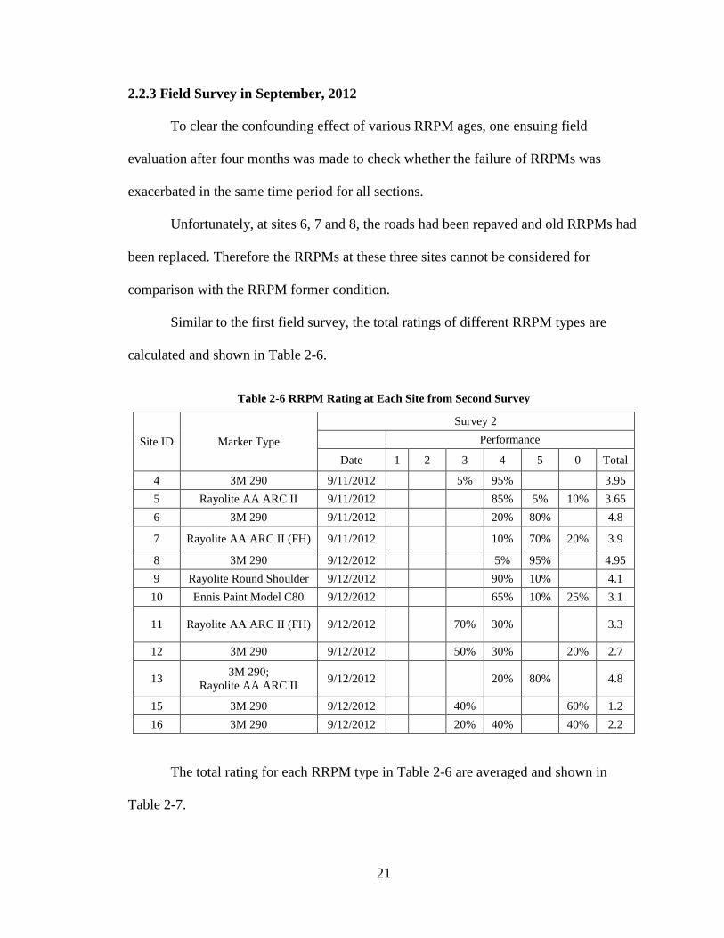
Similar to the first field survey, the total ratings of different RRPM types are

calculated and shown in Table 2-6.

Table 2-6 RRPM Rating at Each Site from Second Survey

The total rating for each RRPM type in Table 2-6 are averaged and shown in

Table 2-7.

Site ID Marker Type

Survey 2

Performance

Date 1 2 3 4 5 0 Total

4 3M 290 9/11/2012 5% 95% 3.95

5 Rayolite AA ARC II 9/11/2012 85% 5% 10% 3.65

6 3M 290 9/11/2012 20% 80% 4.8

7 Rayolite AA ARC II (FH) 9/11/2012 10% 70% 20% 3.9

8 3M 290 9/12/2012 5% 95% 4.95

9 Rayolite Round Shoulder 9/12/2012 90% 10% 4.1

10 Ennis Paint Model C80 9/12/2012 65% 10% 25% 3.1

11 Rayolite AA ARC II (FH) 9/12/2012 70% 30% 3.3

12 3M 290 9/12/2012 50% 30% 20% 2.7

13 3M 290;

Rayolite AA ARC II 9/12/2012 20% 80% 4.8

15 3M 290 9/12/2012 40% 60% 1.2

16 3M 290 9/12/2012 20% 40% 40% 2.2

22

Table 2-7 Average Ratings of Various RRPM Types from Second Survey

Marker Type Average Rating

3M 290 3.51

Rayolite AA ARC II 3.9

Rayolite Round Shoulder 4.1

Ennis Paint Model C80 3.1

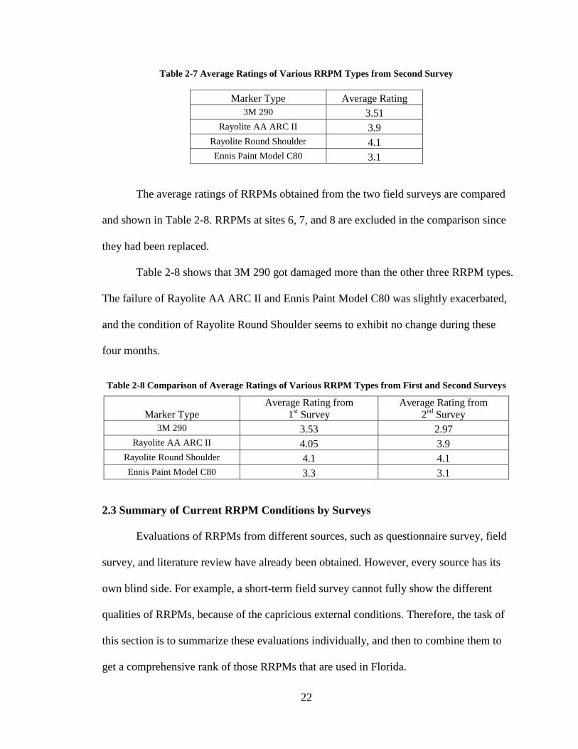
The average ratings of RRPMs obtained from the two field surveys are compared

and shown in Table 2-8. RRPMs at sites 6, 7, and 8 are excluded in the comparison since

they had been replaced.

Table 2-8 shows that 3M 290 got damaged more than the other three RRPM types.

The failure of Rayolite AA ARC II and Ennis Paint Model C80 was slightly exacerbated,

and the condition of Rayolite Round Shoulder seems to exhibit no change during these

four months.

Table 2-8 Comparison of Average Ratings of Various RRPM Types from First and Second Surveys

Marker Type

Average Rating from

1st Survey

Average Rating from

2nd

Survey

3M 290 3.53 2.97

Rayolite AA ARC II 4.05 3.9

Rayolite Round Shoulder 4.1 4.1

Ennis Paint Model C80 3.3 3.1

2.3 Summary of Current RRPM Conditions by Surveys

Evaluations of RRPMs from different sources, such as questionnaire survey, field

survey, and literature review have already been obtained. However, every source has its

own blind side. For example, a short-term field survey cannot fully show the different

qualities of RRPMs, because of the capricious external conditions. Therefore, the task of

this section is to summarize these evaluations individually, and then to combine them to

get a comprehensive rank of those RRPMs that are used in Florida.

23

2.3.1 Questionnaire Survey

This survey directly provides general evaluations of different RRPMs from

experienced engineers and specialists. The results show that 27 percent respondents select

3M 290 as the best type, and the rests have no significant preference. Thus, this

questionnaire survey identifies 3M 290 as better performing than the other types of

RRPMs.

2.3.2 Field Survey

In contrast with the questionnaire survey, field survey provides more details of

RRPM performance. According to rating performances of RRPMs from two field surveys,

which are shown in Table 2-8, the rank of RRPMs is determined as follows: Rayolite RS >

Rayolite AA ARC II >Ennis C80-FH > 3M 290.

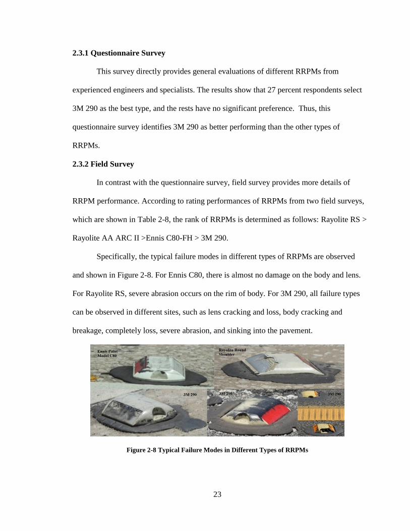
Specifically, the typical failure modes in different types of RRPMs are observed

and shown in Figure 2-8. For Ennis C80, there is almost no damage on the body and lens.

For Rayolite RS, severe abrasion occurs on the rim of body. For 3M 290, all failure types

can be observed in different sites, such as lens cracking and loss, body cracking and

breakage, completely loss, severe abrasion, and sinking into the pavement.

Figure 2-8 Typical Failure Modes in Different Types of RRPMs

24

2.3.3 Manufacturers’ Information

Manufacturers also provide some related information about their products.

However, to avoid bias, this part only compares two RRPMs manufactured from the

same company. In Florida, only Ennis’ two different RRPM modes are approved in the

QPL. Ennis states that Ennis 980 marker is a new product which has higher performance

and durability than their former products. It seems that Ennis 980 is the next generation

of Ennis C80. Therefore, it is safe to say that Ennis 980 is more advanced than Ennis C80.

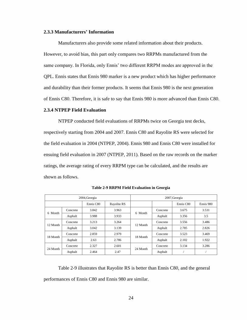
2.3.4 NTPEP Field Evaluation

NTPEP conducted field evaluations of RRPMs twice on Georgia test decks,

respectively starting from 2004 and 2007. Ennis C80 and Rayolite RS were selected for

the field evaluation in 2004 (NTPEP, 2004). Ennis 980 and Ennis C80 were installed for

ensuing field evaluation in 2007 (NTPEP, 2011). Based on the raw records on the marker

ratings, the average rating of every RRPM type can be calculated, and the results are

shown as follows.

Table 2-9 RRPM Field Evaluation in Georgia

2004,Georgia 2007,Georgia

Ennis C80 Rayolite RS Ennis C80 Ennis 980

6 Month Concrete 3.842 3.963


Asphalt 3.988 3.933 Asphalt 3.356 3.5



Asphalt 3.042 3.139 Asphalt 2.785 2.826



Asphalt 2.63 2.786 Asphalt 2.102 1.922



Asphalt 2.464 2.47 Asphalt / /

Table 2-9 illustrates that Rayolite RS is better than Ennis C80, and the general

performances of Ennis C80 and Ennis 980 are similar.

25

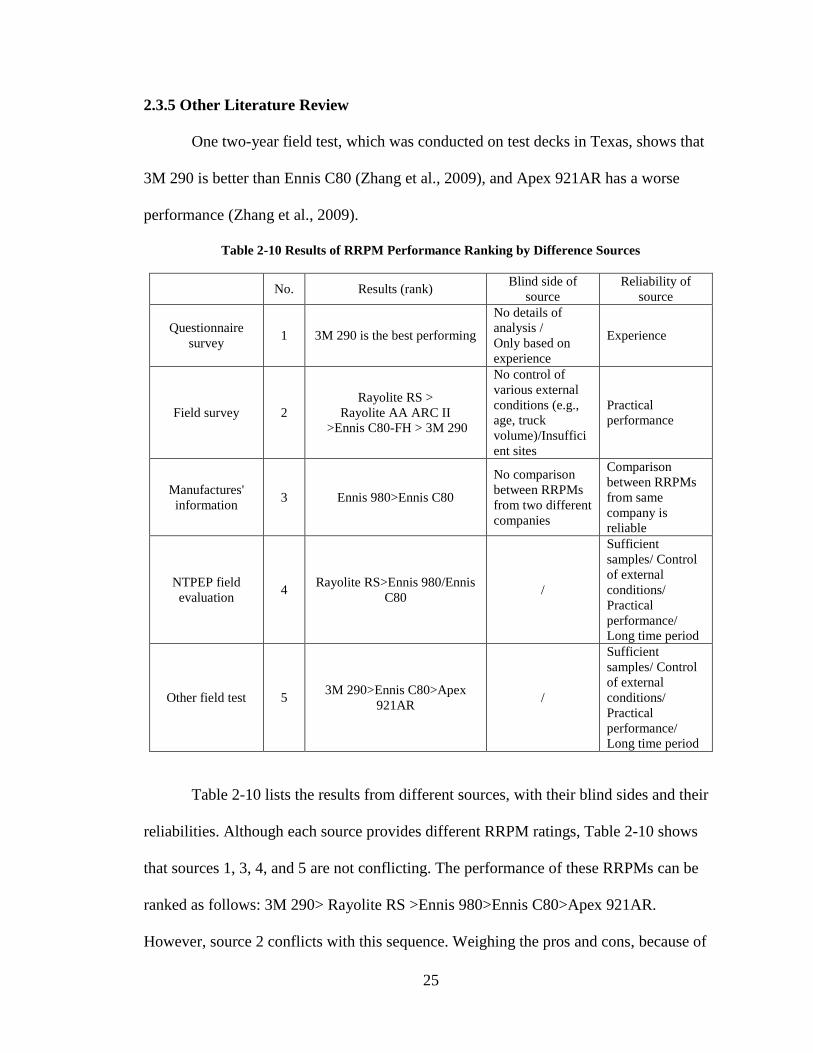
2.3.5 Other Literature Review

One two-year field test, which was conducted on test decks in Texas, shows that

3M 290 is better than Ennis C80 (Zhang et al., 2009), and Apex 921AR has a worse

performance (Zhang et al., 2009).

Table 2-10 Results of RRPM Performance Ranking by Difference Sources

No. Results (rank) Blind side of

source

Reliability of

source

Questionnaire

survey 1 3M 290 is the best performing

No details of

analysis /

Only based on

experience

Experience

Field survey 2

Rayolite RS >

Rayolite AA ARC II

>Ennis C80-FH > 3M 290

No control of

various external

conditions (e.g.,

age, truck

volume)/Insuffici

ent sites

Practical

performance

Manufactures'

information 3 Ennis 980>Ennis C80

No comparison

between RRPMs

from two different

companies

Comparison

between RRPMs

from same

company is

reliable

NTPEP field

evaluation 4

Rayolite RS>Ennis 980/Ennis

C80 /

Sufficient

samples/ Control

of external

conditions/

Practical

performance/

Long time period

Other field test 5 3M 290>Ennis C80>Apex

921AR /

Sufficient

samples/ Control

of external

conditions/

Practical

performance/

Long time period

Table 2-10 lists the results from different sources, with their blind sides and their

reliabilities. Although each source provides different RRPM ratings, Table 2-10 shows

that sources 1, 3, 4, and 5 are not conflicting. The performance of these RRPMs can be

ranked as follows: 3M 290> Rayolite RS >Ennis 980>Ennis C80>Apex 921AR.

However, source 2 conflicts with this sequence. Weighing the pros and cons, because of

26

their severe blind sides which are listed in Table 2-10, the ranking from source 2 is

ignored. The result of source 2 also illustrates that the RRPM performance significantly

depends on the external conditions.

As the final consequence, the estimated rank of RRPMs in Florida can be

expressed as: 3M 290> Rayolite RS >Ennis 980>Ennis C80>Apex 921AR.

27

CHAPTER 3: METHODOLOGY

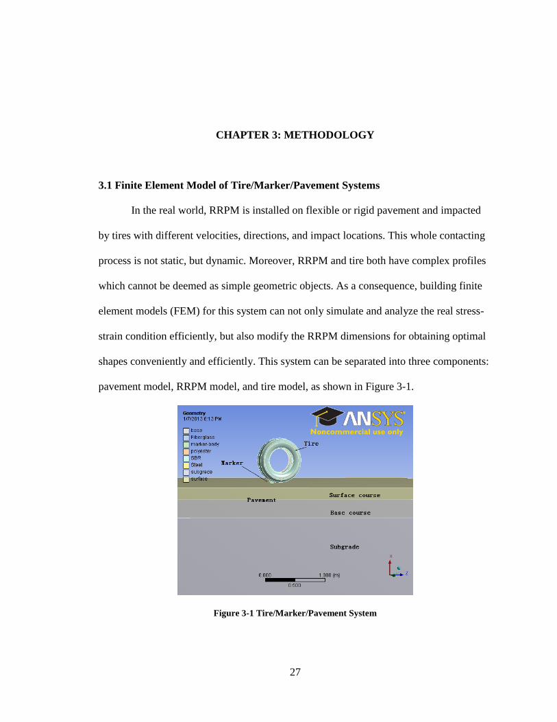
3.1 Finite Element Model of Tire/Marker/Pavement Systems

In the real world, RRPM is installed on flexible or rigid pavement and impacted

by tires with different velocities, directions, and impact locations. This whole contacting

process is not static, but dynamic. Moreover, RRPM and tire both have complex profiles

which cannot be deemed as simple geometric objects. As a consequence, building finite

element models (FEM) for this system can not only simulate and analyze the real stress-

strain condition efficiently, but also modify the RRPM dimensions for obtaining optimal

shapes conveniently and efficiently. This system can be separated into three components:

pavement model, RRPM model, and tire model, as shown in Figure 3-1.

Figure 3-1 Tire/Marker/Pavement System

28

3.1.1 Pavement Model

Normally, pavement has two categories: flexible and rigid. For flexible one, it

typically consists of three layers: surface of asphalt, base and subgrade courses of

aggregates and soil. For rigid one, the surface is portland cement concrete instead and

may be without base course. Because questionnaire and field surveys involve mainly

flexible pavements in Florida, only flexible one is considered in this study. The following

characteristics of a pavement model is obtained by Texas Transportation Institute (TTI)

researchers and used in this study (Zhang et al., 2009). This pavement model matches the

geometric designs of interstate highways bearing a large percentage of heavy traffic

volume.

Table 3-1 Profiles and Material Properties for Flexible Pavement

Layer name Thickness (m) Density (kg/m3) Poisson’s Ratio Young’s

Modulus (MPa)

Surface 0.2 2322 0.35 3000

Base 0.3 2162 0.35 300

Subgrade 5.0 2001 0.35 10

3.1.2 Tire Model

Tire model, used in this paper, was previously developed by a USF investigation

team for studying Locked Wheel Skid Tester (LWST) (Kosgolla, 2012). The cross

sectional profile of this tire model is derived by slicing a spent standard ASTM E524-08

tire. This tire model consists of two fiberglass belted plies, two polymer biased plies,

steel beads and tire rubber. As the main tire component contributing to friction, a tire

rubber with styrene butadiene rubber (SBR) has both hyperelastic and viscoelastic

properties. In ANSYS 12.0, Mooney-Revlin model can be developed for hyperelastic

29

property, and Prony series model can be applied for viscoelastic property. These relevant

material properties and empirical constants are achieved from previous ASTM studies

(ASTM 2001; ASTM 2006). Based on the above information, a three-dimension tire

model is constructed in SolidWorks 2010 software, and then imported to the ANSYS

platform for providing dynamic impact to RRPM.

3.1.3 RRPM Model

3.1.3.1 Details of RRPM Geometric Characteristics

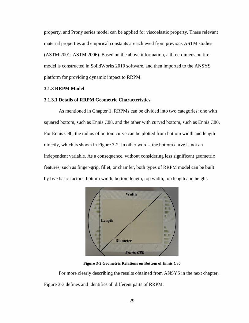
As mentioned in Chapter 1, RRPMs can be divided into two categories: one with

squared bottom, such as Ennis C88, and the other with curved bottom, such as Ennis C80.

For Ennis C80, the radius of bottom curve can be plotted from bottom width and length

directly, which is shown in Figure 3-2. In other words, the bottom curve is not an

independent variable. As a consequence, without considering less significant geometric

features, such as finger-grip, fillet, or chamfer, both types of RRPM model can be built

by five basic factors: bottom width, bottom length, top width, top length and height.

Figure 3-2 Geometric Relations on Bottom of Ennis C80

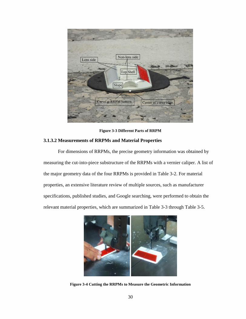
For more clearly describing the results obtained from ANSYS in the next chapter,

Figure 3-3 defines and identifies all different parts of RRPM.

30

Figure 3-3 Different Parts of RRPM

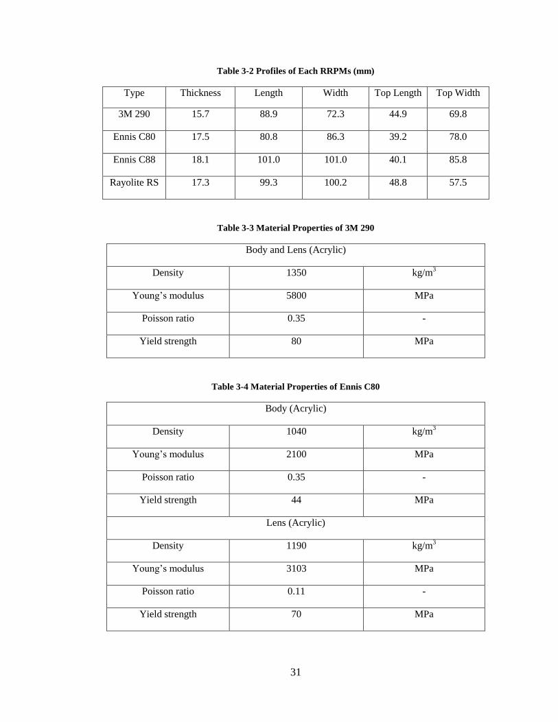
3.1.3.2 Measurements of RRPMs and Material Properties

For dimensions of RRPMs, the precise geometry information was obtained by

measuring the cut-into-piece substructure of the RRPMs with a vernier caliper. A list of

the major geometry data of the four RRPMs is provided in Table 3-2. For material

properties, an extensive literature review of multiple sources, such as manufacturer

specifications, published studies, and Google searching, were performed to obtain the

relevant material properties, which are summarized in Table 3-3 through Table 3-5.

Figure 3-4 Cutting the RRPMs to Measure the Geometric Information

31

Table 3-2 Profiles of Each RRPMs (mm)

Type Thickness Length Width Top Length Top Width

3M 290 15.7 88.9 72.3 44.9 69.8

Ennis C80 17.5 80.8 86.3 39.2 78.0

Ennis C88 18.1 101.0 101.0 40.1 85.8

Rayolite RS 17.3 99.3 100.2 48.8 57.5

Table 3-3 Material Properties of 3M 290

Body and Lens (Acrylic)

Density 1350 kg/m3

Young’s modulus 5800 MPa

Poisson ratio 0.35 -

Yield strength 80 MPa

Table 3-4 Material Properties of Ennis C80

Body (Acrylic)

Density 1040 kg/m3




Lens (Acrylic)

Density 1190 kg/m3




32

Table 3-5 Material Properties of Rayolite RS

Filler (Inert Thermosetting Compound)

Density kg/m3



Yield strength MPa

Housing (Acrylonitrile Butadiene Stryrene )

Density kg/m3



Yield strength MPa

Lens ( Methyl Methcrylate )

Density kg/m3



Yield strength MPa

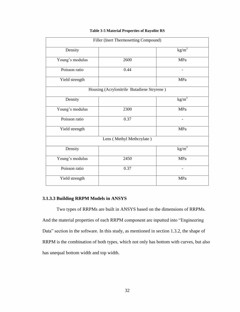
3.1.3.3 Building RRPM Models in ANSYS

Two types of RRPMs are built in ANSYS based on the dimensions of RRPMs.

And the material properties of each RRPM component are inputted into “Engineering

Data” section in the software. In this study, as mentioned in section 1.3.2, the shape of

RRPM is the combination of both types, which not only has bottom with curves, but also

has unequal bottom width and top width.

33

Figure 3-5 RRPM Model in ANSYS

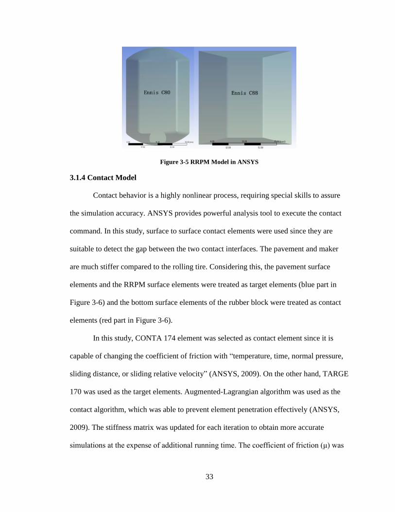
3.1.4 Contact Model

Contact behavior is a highly nonlinear process, requiring special skills to assure

the simulation accuracy. ANSYS provides powerful analysis tool to execute the contact

command. In this study, surface to surface contact elements were used since they are

suitable to detect the gap between the two contact interfaces. The pavement and maker

are much stiffer compared to the rolling tire. Considering this, the pavement surface

elements and the RRPM surface elements were treated as target elements (blue part in

Figure 3-6) and the bottom surface elements of the rubber block were treated as contact

elements (red part in Figure 3-6).

In this study, CONTA 174 element was selected as contact element since it is

capable of changing the coefficient of friction with “temperature, time, normal pressure,

sliding distance, or sliding relative velocity” (ANSYS, 2009). On the other hand, TARGE

170 was used as the target elements. Augmented-Lagrangian algorithm was used as the

contact algorithm, which was able to prevent element penetration effectively (ANSYS,

2009). The stiffness matrix was updated for each iteration to obtain more accurate

simulations at the expense of additional running time. The coefficient of friction (μ) was

34

defined using the Coulomb friction model and in the modeling, field surveyed value was

used (ANSYS, 2009).

Figure 3-6 Tire-Marker Contact System

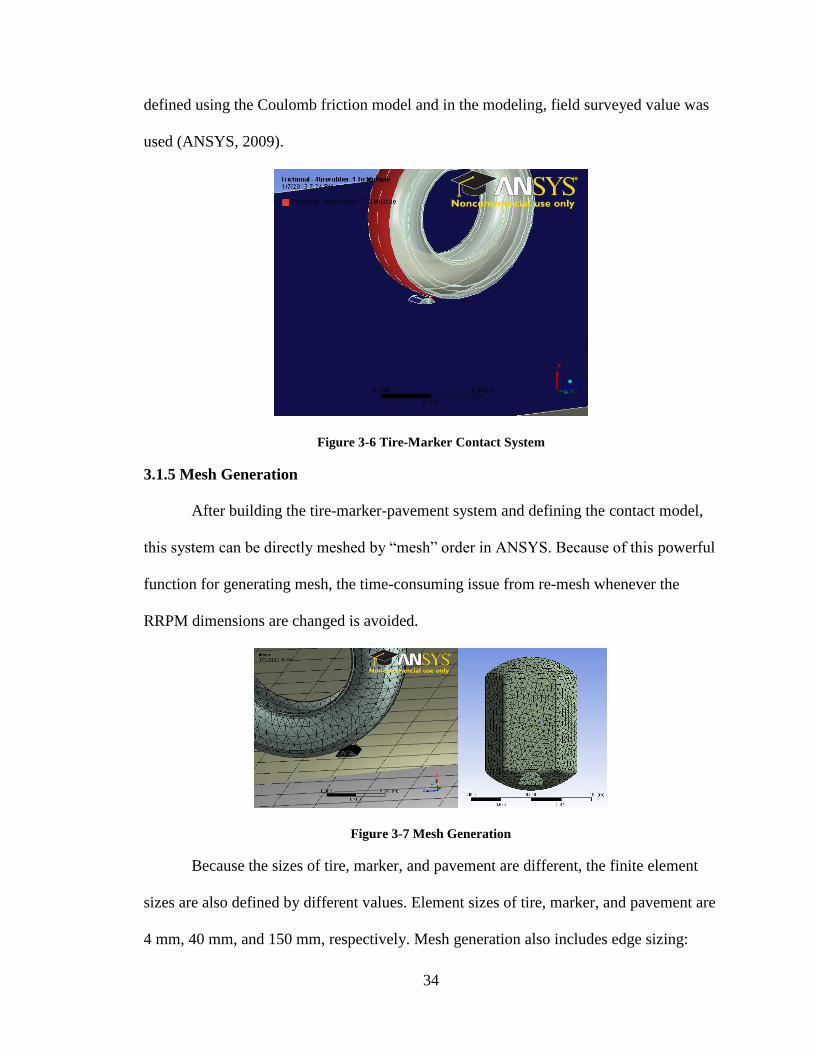
3.1.5 Mesh Generation

After building the tire-marker-pavement system and defining the contact model,

this system can be directly meshed by “mesh” order in ANSYS. Because of this powerful

function for generating mesh, the time-consuming issue from re-mesh whenever the

RRPM dimensions are changed is avoided.

Figure 3-7 Mesh Generation

Because the sizes of tire, marker, and pavement are different, the finite element

sizes are also defined by different values. Element sizes of tire, marker, and pavement are

4 mm, 40 mm, and 150 mm, respectively. Mesh generation also includes edge sizing:

35

eight edges of two pavement layers are selected and every edge is divided by three

divisions.

3.1.6 Finite Element Model Assembly

In this part, the tire is molded to roll over the RRPMs dynamically. Several

external factors, such as tire loading and vehicle velocity, are defined. Because the

federal government limits vehicle weights and speeds on most interstate highways, these

critical values are used in this study to define the tire load and vehicle velocity, which are

22200 N and 31.3m/s, respectively (Zhang et al., 2009). The boundary condition is that

the bottom of sub-grade layer is set as “fixed support” for this system. After defining

these external factors and assembling all the components, the whole system is simulated

in ANSYS.

3.2 Experimental Design

After the completion of the previous work, the researcher continued to examine

the effects of geometric factors—bottom length (BL), top length(TL), bottom width

(BW), top width (TW) and height (H)—on the various stresses inside the markers, such

as von Mises stress, principal stress, shear stress, and normal stress. The reasons of

analyzing these stresses are specifically described in section 3.3. The levels of involved

factors (BL, TL, BW, TW/BW, and H) are listed in Table 3-6.

Table 3-6 Matrix of Test Scenarios

Level Element

BL

(mm)

TL

(mm)

BW

(mm)

TW/BW H

(mm)

Lv. 1 80.2 40.1 64.3 0.85 14

Lv. 2 85.3 42.2 70.5 0.9 15.7

Lv. 3 90 44.6 75.2 0.94 17.5

Lv. 4 95 47.1 80.2 1 19.25

36

It is realized that the entire modeling program would involve 54 1024

combinations of the levels of influencing factors, as shown in Table 3-6, for a full

factorial design. Considering that every simulation takes at least two and a half hours

using ANSYS, conducting all these tests is very much time consuming. To reduce the

simulation work and meanwhile maintain the reliability of conclusions, an orthogonal

design was used.

3.2.1 Orthogonal Design

3.2.1.1 Basic Concept of Orthogonal Design

Orthogonal design (Taguchi method) is a highly fractionated factorial design.

This multi-factor multi-level experimental design selects some representative points from

full-scale test to efficiently observe relationships between factors and effects. Because the

selected points are evenly dispersed and neatly comparable, all interactions between the

controls can be negligible.

Specifically, one typical example of fractional factorial design about four factors

at three levels is introduced in detail as following.

If one experimental design has 4 factors and each factor has 3 levels, a full

factorial design needs 43 81 tests, as shown in Figure 3-8. Compared to the full

factorial design, a fractional factorial design only needs 4 23 9 tests, as shown in Figure

3-9. Although the fractional factorial design omits many tests, it still can express the

integral situation by highly representative tests. These selected tests are distributed evenly,

without any redundancy.

Through fractional factorial design, because of uniform appearance of other

control factors, which can be offset by each other, every factor can be viewed as

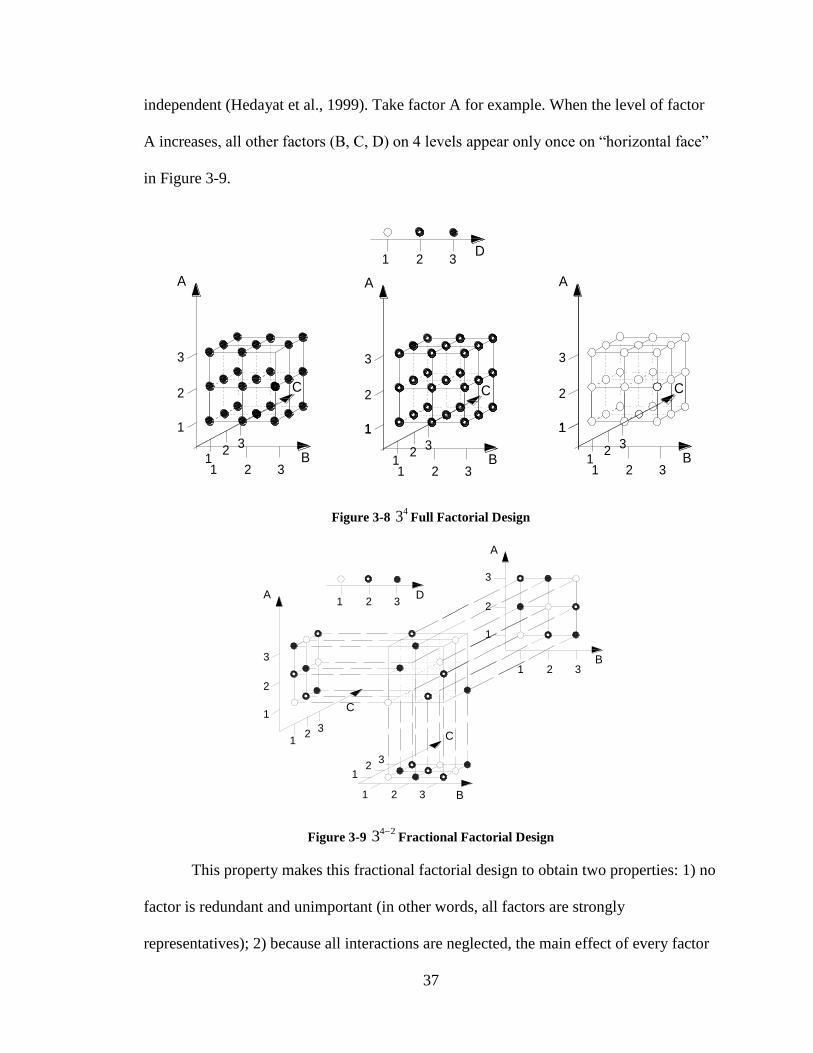
37

independent (Hedayat et al., 1999). Take factor A for example. When the level of factor

A increases, all other factors (B, C, D) on 4 levels appear only once on “horizontal face”

in Figure 3-9.

D1 2 3

A

3

2

1

12

3

C

B1 2 3

1

12

3B

1 2 3

A

3

2

1

C

1

12

3B

1 2 3

11

A

3

2

1

C

Figure 3-8 43 Full Factorial Design

A

A

B

B

C

C

D1 2 3

1 2 3

1 2 3

12

3

3

2

1

3

2

1

12

3

Figure 3-9 4 23

Fractional Factorial Design

This property makes this fractional factorial design to obtain two properties: 1) no

factor is redundant and unimportant (in other words, all factors are strongly

representatives); 2) because all interactions are neglected, the main effect of every factor

38

can be observed individually. This property also makes orthogonal design to lack

information about interactions and the main effects of individual factors are only general

tendency, not accurate enough. So, this fractional factorial design is also termed as

orthogonal main effect design.

The test arrangement in Figure 3-9 can be transferred into Table 3-7.

Table 3-7 Orthogonal Table of 4 2

9 3 L ( )

Factor Level

Test A B C D

1 1 1 1 1

2 1 2 2 2

3 1 3 3 3

4 2 1 2 3

5 2 2 3 1

6 2 3 1 2

7 3 1 3 2

8 3 2 1 3

9 3 3 2 1

For this orthogonal array, all columns can be deemed as vectors, such as A

[1,1,1,2,2,2,3,3,3], B[1,2,3,1,2,3,1,2,3], C[1,2,3,2,3,1,3,1,2], and D[1,2,3,3,1,2,2,3,1].

Mathematically, two vectors are orthogonal when their dot product is zero. Apparently, in

this case, dot product by any two vectors is not zero, but equal. If the codes of three

levels are replaced by -1, 0, and +1, the dot product by any two vectors will be zero. This

is a good method to check whether the fractional factorial design is orthogonal.

For any fractional factorial design, the array can be expressed by the symbol as

OA (N, k, s, t) (Hedayat et al., 1999). Number of tests, factors, and levels are represented

by parameters N, k, and s, respectively. In this case, the orthogonal design can be

described as OA (9, 4, 3, 2).

39

3.2.1.2 Four-level Fractional Factorial Design

The L16 (45-3

) table which was obtained from Sloane’s website is adjusted and

used in this specific situation, with the array listed in Table 3-8. Table 3-8 shows that

every 4 tests are conducted for each factor on each level. Within every 4 tests, other

control variables on different levels appear equally. Taking factor C on level 3 (C3) for

instance, test 3, test 8, test 9 and test 14 are conducted for this specific factor on specific

level. A1 to A4, B1 to B4, D1 to D4 and E1 to E4 all appear only once in these 4 tests.

Hence, the interactive effects are offset, and only the individual effects of each parameter

are considered. Compared to the full factorial design, this four-level fractional factorial

design can save substantial time and avoid redundancy.


)

Factor

Test A B C D E

1 A4 B1 C1 D1 E1

2 A4 B2 C2 D2 E2

3 A4 B3 C3 D3 E3

4 A4 B4 C4 D4 E4

5 A1 B1 C2 D3 E4

6 A1 B2 C1 D4 E3

7 A1 B3 C4 D1 E2

8 A1 B4 C3 D2 E1

9 A2 B1 C3 D4 E2

10 A2 B2 C4 D3 E1

11 A2 B3 C1 D2 E4

12 A2 B4 C2 D1 E3

13 A3 B1 C4 D2 E3

14 A3 B2 C3 D1 E4

15 A3 B3 C2 D4 E1

16 A3 B4 C1 D3 E2

40

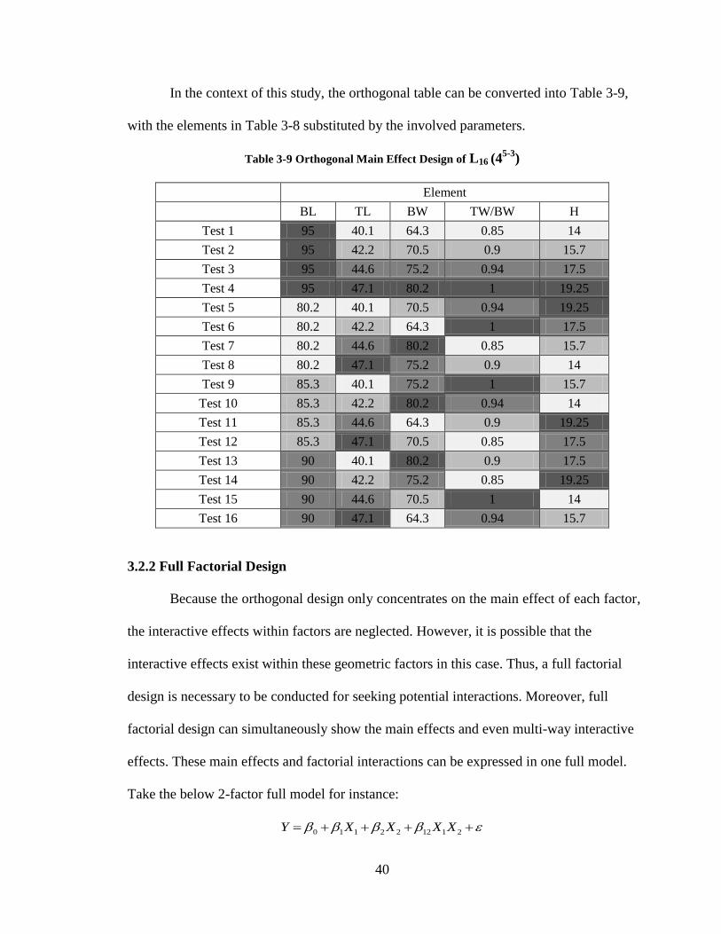
In the context of this study, the orthogonal table can be converted into Table 3-9,

with the elements in Table 3-8 substituted by the involved parameters.

Table 3-9 Orthogonal Main Effect Design of L16 (45-3

)

Element

BL TL BW TW/BW H

Test 1 95 40.1 64.3 0.85 14

Test 2 95 42.2 70.5 0.9 15.7

Test 3 95 44.6 75.2 0.94 17.5

Test 4 95 47.1 80.2 1 19.25

Test 5 80.2 40.1 70.5 0.94 19.25

Test 6 80.2 42.2 64.3 1 17.5

Test 7 80.2 44.6 80.2 0.85 15.7

Test 8 80.2 47.1 75.2 0.9 14

Test 9 85.3 40.1 75.2 1 15.7

Test 10 85.3 42.2 80.2 0.94 14

Test 11 85.3 44.6 64.3 0.9 19.25

Test 12 85.3 47.1 70.5 0.85 17.5

Test 13 90 40.1 80.2 0.9 17.5

Test 14 90 42.2 75.2 0.85 19.25

Test 15 90 44.6 70.5 1 14

Test 16 90 47.1 64.3 0.94 15.7

3.2.2 Full Factorial Design

Because the orthogonal design only concentrates on the main effect of each factor,

the interactive effects within factors are neglected. However, it is possible that the

interactive effects exist within these geometric factors in this case. Thus, a full factorial

design is necessary to be conducted for seeking potential interactions. Moreover, full

factorial design can simultaneously show the main effects and even multi-way interactive

effects. These main effects and factorial interactions can be expressed in one full model.

Take the below 2-factor full model for instance:

0 1 1 2 2 12 1 2Y X X X X

41

In this full factorial model, β12 represents the interactive effect; β1and β2

respectively indicate the main effect of X1 and X2 (Hill and Lewicki, 2006). The

researcher can use ANOVA in statistical software, such as SPSS, to analyze the main

effects and interaction effects of these factors. Moreover, statistically, all “beta”

coefficients, R-squared, t value can be obtained and then used to check some conclusions.

For example, if t value of X1 X2 is larger than critical value, β12 means one variable does

significantly influence the effect of another variable on response Y (Hill and Lewicki,

2006). Because full factorial design in this study is based on the results of fractional

factorial design, the details of full factorial design are described later.

3.3 Stress Indicators Determination

Questionnaire survey and field survey show that RRPM suffers different failure

modes under different scenarios. These failures happen on the various locations, such as

top edges, top shell, and bottom surface of RRPM. In this study, four types of stresses,

including von Mises stress, principal stress, shear stress on bottom, and normal stress on

bottom, are analyzed to figure out which stress causes which specific failure mode. The

results also can indirectly illustrate the relationship between the RRPM geometric

characteristics and their failure modes.

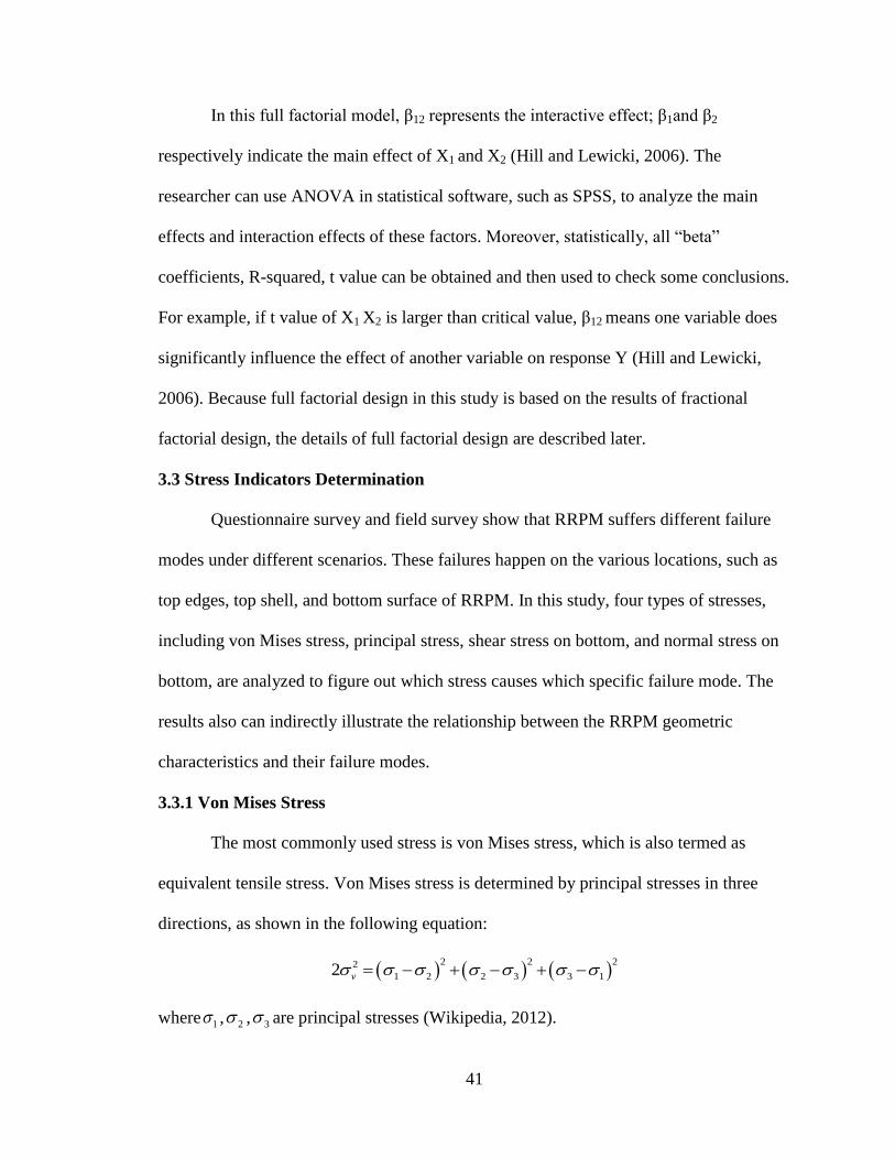
3.3.1 Von Mises Stress

The most commonly used stress is von Mises stress, which is also termed as

equivalent tensile stress. Von Mises stress is determined by principal stresses in three

directions, as shown in the following equation:

2 2 22

1 2 2 3 3 12 v

where 1 , 2 , 3 are principal stresses (Wikipedia, 2012).

42

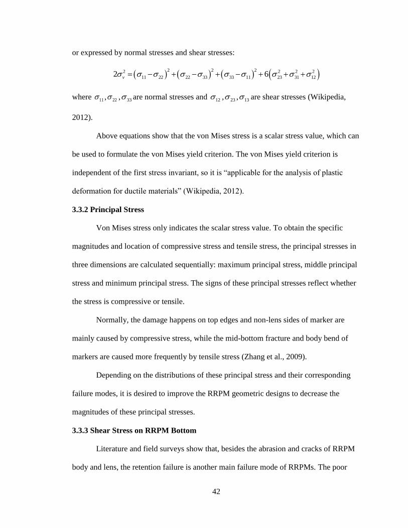
or expressed by normal stresses and shear stresses:

2 2 22 2 2 2

11 22 22 33 33 11 23 31 122 6v

where 11 , 22 , 33 are normal stresses and 12 , 23 , 13 are shear stresses (Wikipedia,

2012).

Above equations show that the von Mises stress is a scalar stress value, which can

be used to formulate the von Mises yield criterion. The von Mises yield criterion is

independent of the first stress invariant, so it is “applicable for the analysis of plastic

deformation for ductile materials” (Wikipedia, 2012).

3.3.2 Principal Stress

Von Mises stress only indicates the scalar stress value. To obtain the specific

magnitudes and location of compressive stress and tensile stress, the principal stresses in

three dimensions are calculated sequentially: maximum principal stress, middle principal

stress and minimum principal stress. The signs of these principal stresses reflect whether

the stress is compressive or tensile.

Normally, the damage happens on top edges and non-lens sides of marker are

mainly caused by compressive stress, while the mid-bottom fracture and body bend of

markers are caused more frequently by tensile stress (Zhang et al., 2009).

Depending on the distributions of these principal stress and their corresponding

failure modes, it is desired to improve the RRPM geometric designs to decrease the

magnitudes of these principal stresses.

3.3.3 Shear Stress on RRPM Bottom

Literature and field surveys show that, besides the abrasion and cracks of RRPM

body and lens, the retention failure is another main failure mode of RRPMs. The poor

43

retention performance is mainly caused by shear stress, which is introduced by impact

from high-speed moving vehicles. This shear stress occurs on the interface of marker and

adhesive. In this study, the shear stress on the RRPM bottom face is calculated.

3.3.4 Normal Stress on RRPM Bottom

Similar to shear stress damage, the damage caused by normal stress also cripples

the RRPM service life significantly, which is especially manifested as sinking into

flexible surface of asphalt concrete pavement. Moreover, normal stress at RRPM bottom

may cause tensile failure. Therefore, quantification of normal stress at RRPM bottom is

very necessary, not only to prevent sinking, but also to avoid detachment.

44

CHAPTER 4: ANALYSIS OF SIMULATION RESULTS

Based on the main methodologies which are introduced in Chapter 3, the

relationship between stresses, failure modes, and RRPM profiles can be connected. As

reflected in Figure 4-1 to Figure 4-6, the magnitudes and locations of various stresses are

shown in the snapshots of the FEM of RRPMs of different sizes. Then, these figures are

compared with the images taken from field survey to deduce the relations between stress

and failure modes. After constructing the connection between stresses and failure modes,

statistical analysis of simulation results are made to suggest any relationship between the

stresses and geometric parameters. According to the connections between stresses, failure

modes, and RRPM profiles, this chapter finally provides some geometrical

countermeasures for the specific failure modes.

4.1 Magnitudes and Distributions of Stresses on RRPMs

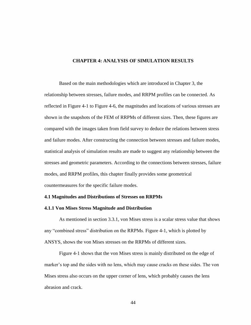
4.1.1 Von Mises Stress Magnitude and Distribution

As mentioned in section 3.3.1, von Mises stress is a scalar stress value that shows

any “combined stress” distribution on the RRPMs. Figure 4-1, which is plotted by

ANSYS, shows the von Mises stresses on the RRPMs of different sizes.

Figure 4-1 shows that the von Mises stress is mainly distributed on the edge of

marker’s top and the sides with no lens, which may cause cracks on these sides. The von

Mises stress also occurs on the upper corner of lens, which probably causes the lens

abrasion and crack.

45

Figure 4-1 Von Mises Stress Distribution

The von Mises stress magnitude is ranging from 150MPa to 300MPa. The

distribution patterns of von Mises stress do not change significantly when the RRPM size

changes.

For more clearly understanding the von Mises stress distribution, the

deformations of RRPM and tire are also plotted by ANSYS, shown in Figure 4-2. Figure

4-2 illustrates why von Mises stress concentrates on the no-lens sides of marker’s top

shell: the deformation of tire is concave-up and it makes the tire surface contact with the

marker on the no-lens sides of marker’s top shell.

Figure 4-2 Deformations of Tire and RRPM

46

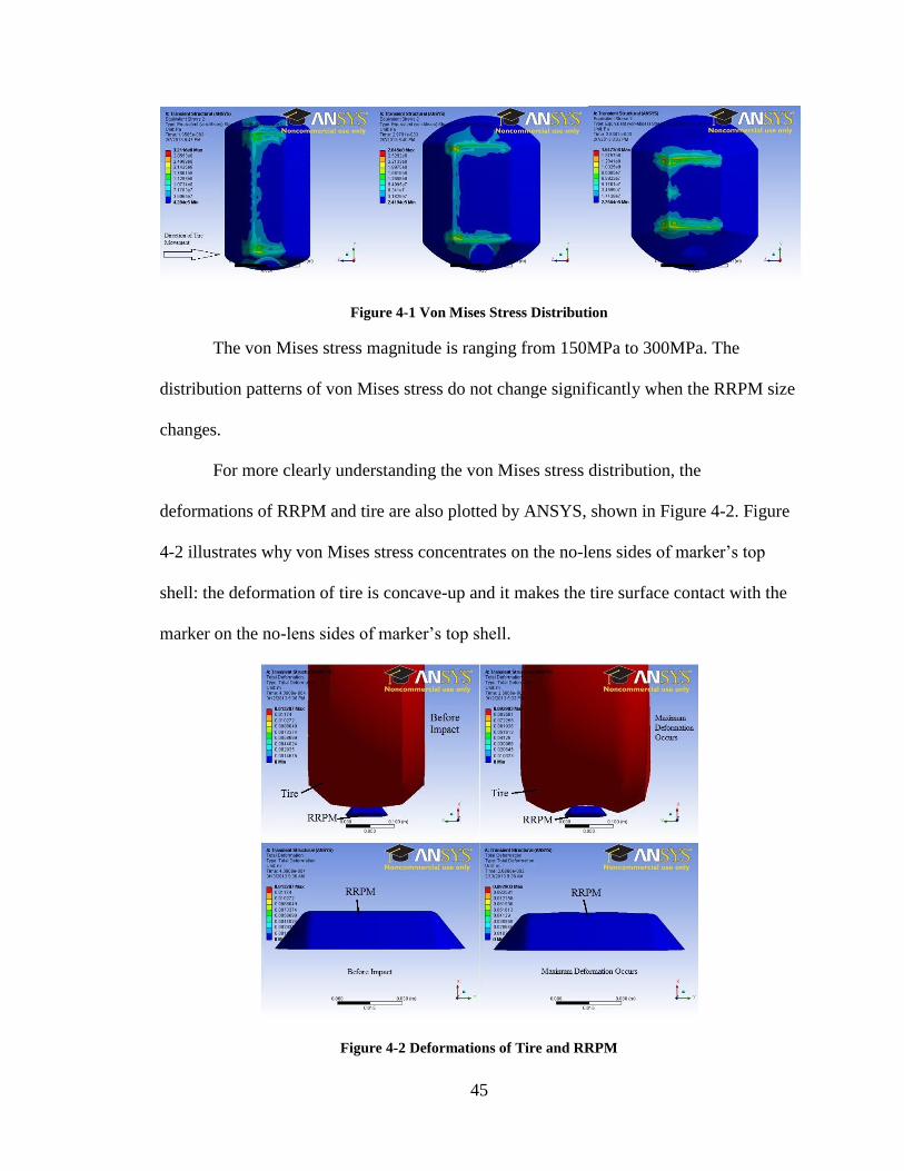
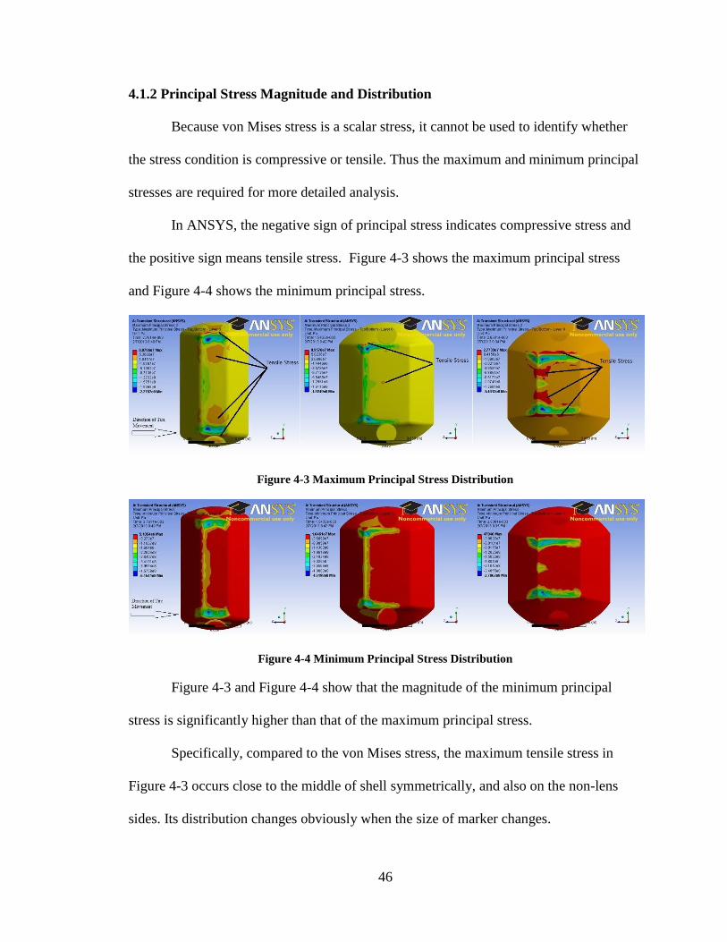
4.1.2 Principal Stress Magnitude and Distribution

Because von Mises stress is a scalar stress, it cannot be used to identify whether

the stress condition is compressive or tensile. Thus the maximum and minimum principal

stresses are required for more detailed analysis.

In ANSYS, the negative sign of principal stress indicates compressive stress and

the positive sign means tensile stress. Figure 4-3 shows the maximum principal stress

and Figure 4-4 shows the minimum principal stress.

Figure 4-3 Maximum Principal Stress Distribution

Figure 4-4 Minimum Principal Stress Distribution

Figure 4-3 and Figure 4-4 show that the magnitude of the minimum principal

stress is significantly higher than that of the maximum principal stress.

Specifically, compared to the von Mises stress, the maximum tensile stress in

Figure 4-3 occurs close to the middle of shell symmetrically, and also on the non-lens

sides. Its distribution changes obviously when the size of marker changes.

47

The minimum principal stress distribution is similar to the distribution of von

Mises stress. Because the magnitudes of compressive stress are noticeably larger than

those of tensile stress, the lowest compressive stress and the highest tensile stress both are

expressed in red color in ANSYS, and thus cannot be identified from each other clearly in

Figure 4-4.

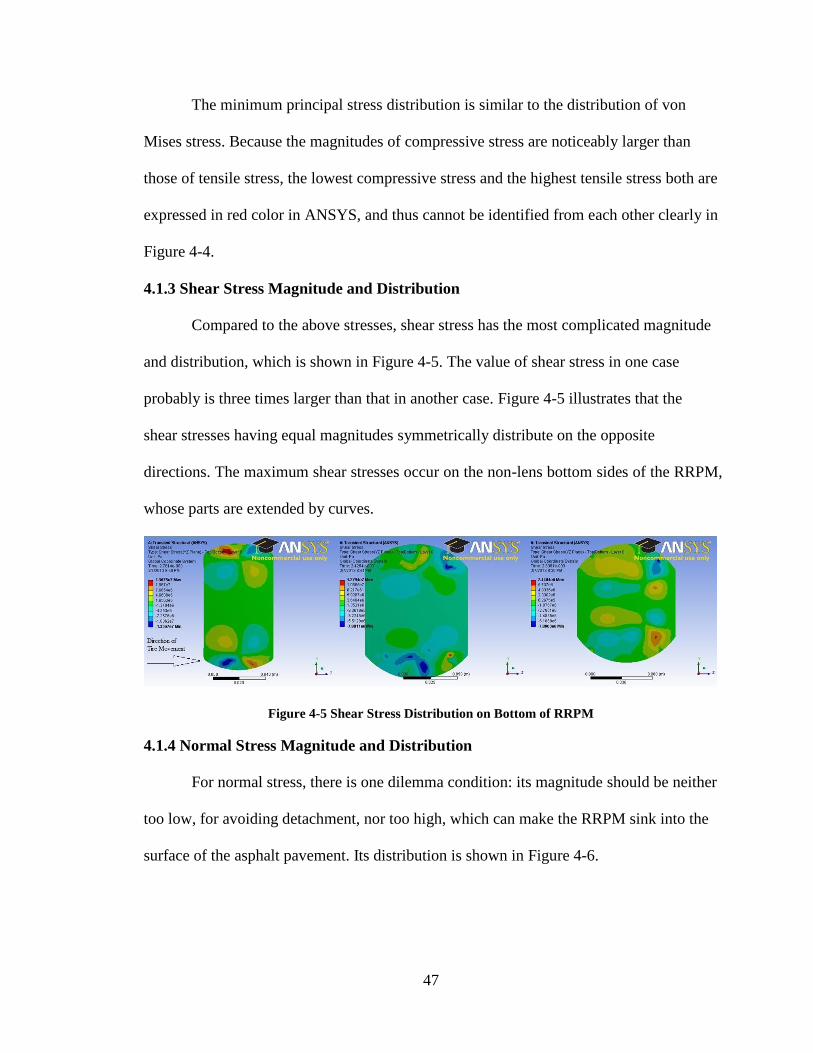
4.1.3 Shear Stress Magnitude and Distribution

Compared to the above stresses, shear stress has the most complicated magnitude

and distribution, which is shown in Figure 4-5. The value of shear stress in one case

probably is three times larger than that in another case. Figure 4-5 illustrates that the

shear stresses having equal magnitudes symmetrically distribute on the opposite

directions. The maximum shear stresses occur on the non-lens bottom sides of the RRPM,

whose parts are extended by curves.

Figure 4-5 Shear Stress Distribution on Bottom of RRPM

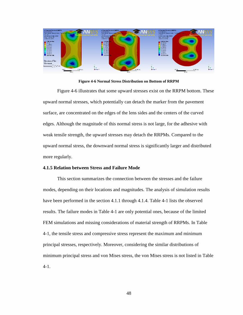
4.1.4 Normal Stress Magnitude and Distribution

For normal stress, there is one dilemma condition: its magnitude should be neither

too low, for avoiding detachment, nor too high, which can make the RRPM sink into the

surface of the asphalt pavement. Its distribution is shown in Figure 4-6.

48

Figure 4-6 Normal Stress Distribution on Bottom of RRPM

Figure 4-6 illustrates that some upward stresses exist on the RRPM bottom. These

upward normal stresses, which potentially can detach the marker from the pavement

surface, are concentrated on the edges of the lens sides and the centers of the curved

edges. Although the magnitude of this normal stress is not large, for the adhesive with

weak tensile strength, the upward stresses may detach the RRPMs. Compared to the

upward normal stress, the downward normal stress is significantly larger and distributed

more regularly.

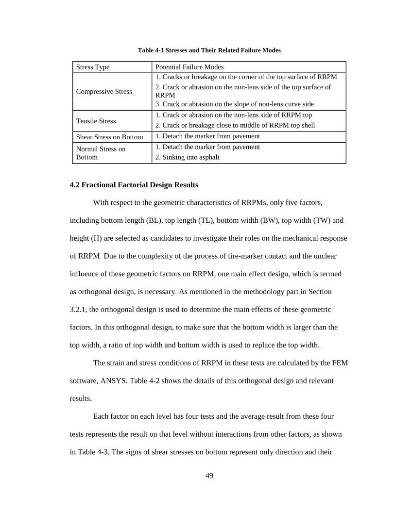
4.1.5 Relation between Stress and Failure Mode

This section summarizes the connection between the stresses and the failure

modes, depending on their locations and magnitudes. The analysis of simulation results

have been performed in the section 4.1.1 through 4.1.4. Table 4-1 lists the observed

results. The failure modes in Table 4-1 are only potential ones, because of the limited

FEM simulations and missing considerations of material strength of RRPMs. In Table

4-1, the tensile stress and compressive stress represent the maximum and minimum

principal stresses, respectively. Moreover, considering the similar distributions of

minimum principal stress and von Mises stress, the von Mises stress is not listed in Table

4-1.

49

Table 4-1 Stresses and Their Related Failure Modes

Stress Type Potential Failure Modes

Compressive Stress

1. Cracks or breakage on the corner of the top surface of RRPM

2. Crack or abrasion on the non-lens side of the top surface of

RRPM

3. Crack or abrasion on the slope of non-lens curve side

Tensile Stress 1. Crack or abrasion on the non-lens side of RRPM top

2. Crack or breakage close to middle of RRPM top shell

Shear Stress on Bottom 1. Detach the marker from pavement

Normal Stress on

Bottom

1. Detach the marker from pavement

2. Sinking into asphalt

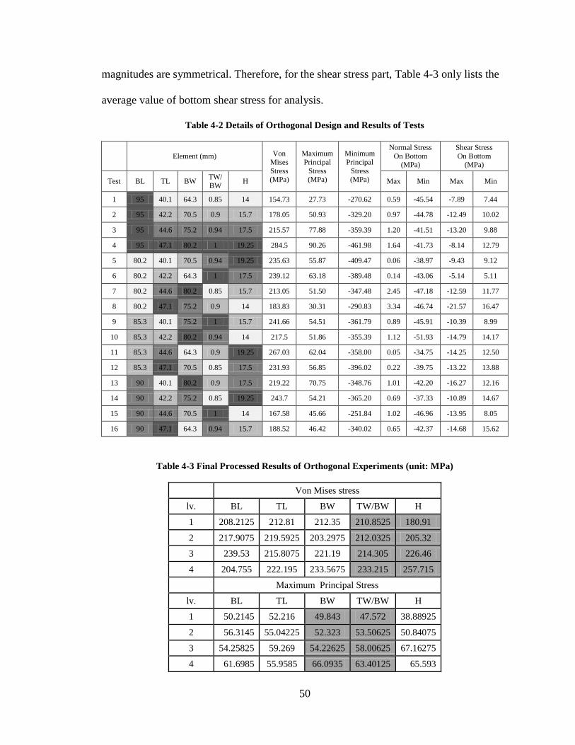
4.2 Fractional Factorial Design Results

With respect to the geometric characteristics of RRPMs, only five factors,

including bottom length (BL), top length (TL), bottom width (BW), top width (TW) and

height (H) are selected as candidates to investigate their roles on the mechanical response

of RRPM. Due to the complexity of the process of tire-marker contact and the unclear

influence of these geometric factors on RRPM, one main effect design, which is termed

as orthogonal design, is necessary. As mentioned in the methodology part in Section

3.2.1, the orthogonal design is used to determine the main effects of these geometric

factors. In this orthogonal design, to make sure that the bottom width is larger than the

top width, a ratio of top width and bottom width is used to replace the top width.

The strain and stress conditions of RRPM in these tests are calculated by the FEM

software, ANSYS. Table 4-2 shows the details of this orthogonal design and relevant

results.

Each factor on each level has four tests and the average result from these four

tests represents the result on that level without interactions from other factors, as shown

in Table 4-3. The signs of shear stresses on bottom represent only direction and their

50

magnitudes are symmetrical. Therefore, for the shear stress part, Table 4-3 only lists the

average value of bottom shear stress for analysis.

Table 4-2 Details of Orthogonal Design and Results of Tests

Element (mm) Von

Mises

Stress (MPa)

Maximum

Principal

Stress (MPa)

Minimum

Principal

Stress (MPa)

Normal Stress

On Bottom (MPa)

Shear Stress

On Bottom (MPa)

Test BL TL BW TW/

BW H Max Min Max Min

1 95 40.1 64.3 0.85 14 154.73 27.73 -270.62 0.59 -45.54 -7.89 7.44

2 95 42.2 70.5 0.9 15.7 178.05 50.93 -329.20 0.97 -44.78 -12.49 10.02

3 95 44.6 75.2 0.94 17.5 215.57 77.88 -359.39 1.20 -41.51 -13.20 9.88

4 95 47.1 80.2 1 19.25 284.5 90.26 -461.98 1.64 -41.73 -8.14 12.79

5 80.2 40.1 70.5 0.94 19.25 235.63 55.87 -409.47 0.06 -38.97 -9.43 9.12

6 80.2 42.2 64.3 1 17.5 239.12 63.18 -389.48 0.14 -43.06 -5.14 5.11

7 80.2 44.6 80.2 0.85 15.7 213.05 51.50 -347.48 2.45 -47.18 -12.59 11.77

8 80.2 47.1 75.2 0.9 14 183.83 30.31 -290.83 3.34 -46.74 -21.57 16.47

9 85.3 40.1 75.2 1 15.7 241.66 54.51 -361.79 0.89 -45.91 -10.39 8.99

10 85.3 42.2 80.2 0.94 14 217.5 51.86 -355.39 1.12 -51.93 -14.79 14.17

11 85.3 44.6 64.3 0.9 19.25 267.03 62.04 -358.00 0.05 -34.75 -14.25 12.50

12 85.3 47.1 70.5 0.85 17.5 231.93 56.85 -396.02 0.22 -39.75 -13.22 13.88

13 90 40.1 80.2 0.9 17.5 219.22 70.75 -348.76 1.01 -42.20 -16.27 12.16

14 90 42.2 75.2 0.85 19.25 243.7 54.21 -365.20 0.69 -37.33 -10.89 14.67

15 90 44.6 70.5 1 14 167.58 45.66 -251.84 1.02 -46.96 -13.95 8.05

16 90 47.1 64.3 0.94 15.7 188.52 46.42 -340.02 0.65 -42.37 -14.68 15.62

Table 4-3 Final Processed Results of Orthogonal Experiments (unit: MPa)

Von Mises stress

lv. BL TL BW TW/BW H

1 208.2125 212.81 212.35 210.8525 180.91

2 217.9075 219.5925 203.2975 212.0325 205.32

3 239.53 215.8075 221.19 214.305 226.46

4 204.755 222.195 233.5675 233.215 257.715

Maximum Principal Stress


1 50.2145 52.216 49.843 47.572 38.88925

2 56.3145 55.04225 52.323 53.50625 50.84075

3 54.25825 59.269 54.22625 58.00625 67.16275

4 61.6985 55.9585 66.0935 63.40125 65.593

51

Table 4-3 Continued

Minimum Principal Stress


1 -359.315 -347.66 -339.53 -344.83 -292.17

2 -367.8 -359.8175 -346.6325 -331.6975 -344.6225

3 -326.455 -329.1775 -344.3025 -366.0675 -373.4125

4 -355.2975 -372.2125 -378.4025 -366.2725 -398.6625

Normal Stress (Minimum)


1 1.496979 0.635099 0.353364 0.98702 1.516865

2 0.568482 0.726103 0.565426 1.339509 1.23524

3 0.839828 1.176887 1.529635 0.755776 0.64089

4 1.095263 1.462463 1.552125 0.918245 0.607555

Normal Stress (Maximum)


1 1.496979 -43.155 -41.431 -42.448 -47.7905

2 0.568482 -44.2735 -42.6163 -42.117 -45.0618

3 0.839828 -42.602 -42.8693 -43.6943 -41.628

4 1.095263 -42.6448 -45.7588 -44.416 -38.195

Average Shear Stress on Bottom


1 11.3986 10.21018 10.3274 11.54409 13.04086

2 12.77293 10.90919 11.26919 14.465 12.0688

3 13.28565 12.02495 13.25735 12.61046 11.10611

4 10.23286 14.54573 12.8361 9.070488 11.47426

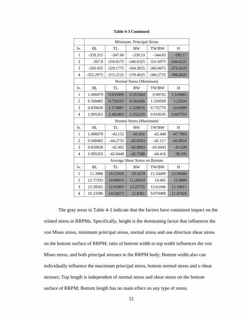
The gray areas in Table 4-3 indicate that the factors have consistent impact on the

related stress in RRPMs. Specifically, height is the dominating factor that influences the

von Mises stress, minimum principal stress, normal stress and one direction shear stress

on the bottom surface of RRPM; ratio of bottom width to top width influences the von

Mises stress, and both principal stresses in the RRPM body; Bottom width also can

individually influence the maximum principal stress, bottom normal stress and o shear

stresses; Top length is independent of normal stress and shear stress on the bottom

surface of RRPM; Bottom length has no main effect on any type of stress.

52

These consistency relations are also shown in Figure 4-7 through Figure 4-12.

The impacts of each factor are plotted to suggest the developing trends. It is worth

pointing out that, although the average shear stress at the bottom surface has no

consistent trends in terms of bottom width and height, the negative shear stress at the

bottom surface is significantly influenced by the bottom width and the positive one has

consistent relationship with height. In this case, these three factors (TL, BW and H) are

all found to significantly influence the shear stress on RRPM bottom. Moreover, because

the sign of minimum principal stress only represents stress direction, for better

observation of magnitude trend, its negative sign is converted into positive one in Figure

4-9.

Figure 4-7 Von Mises Stress vs. Height and Ratio of Top Width and Bottom Width

Figure 4-8 Maximum Principal Stress vs. Bottom Width and Ratio of Top Width and Bottom Width

1 2 3 4

TW/BW 210.8525 212.0325 214.305 233.215

H 180.91 205.32 226.46 257.715

0

50

100

150

200

250

300

Vo

n M

ise

s St

ress

(M

Pa)

53

Figure 4-9 Minimum Principal Stress vs. Height

Figure 4-10 Minimum Normal Stress vs. Height, Top Length, and Bottom Width

Figure 4-11 Maximum Normal Stress vs. Bottom Width and Height

54

Figure 4-12 Shear Stress vs. Bottom Width, Top Length and Height

The results from Figure 4-7 through Figure 4-12 are listed in Table 4-4. In this

table, “+” means positive relation and “–” stands for negative relation. Table 4-4 shows

that decreasing height can reduce von Mises stress and minimum principal stress in

RRPM body. However, decreasing height also causes the increase of normal stress and

shear stress on RRPM bottom. The enlarged bottom width makes maximum principal

stress, normal stress and shear stress increase. The same relation is found between top

length, with minimum normal stress and shear stress. Moreover, the less the ratio of top

width and bottom width is, the less the von Mises stress and maximum principal stress

are.

Table 4-4 Trends of Stress Magnitudes in Terms of Geometric Factors

Stress

Geometric

Factor

Equivalent

Stress

Maximum

Principal

Stress

Minimum

Principal

Stress

Maximum

Normal

Stress

Minimum

Normal

Stress

Shear

Stress

Height +

+ - - -

Ratio of Top

Width

and Bottom

Width + +

Bottom

Width

+

+ + +

Top Length

+ +

Bottom

Length

Level 1 Level 2 Level 3 Level 4

TL 10.21018 10.90919 12.02495 14.54573

BW 10.3274 11.26919 13.25735 12.8361

H 13.04086 12.0688 11.10611 11.47426

0

5

10

15

20

She

ar S

tre

ss o

n

Bo

tto

m (

MP

a)

55

4.3 Full Factorial Design Results

The results of orthogonal design illustrates that the bottom length has no

consistent influence on stresses. However, it is also possible that the length and width

have some interactions, which cause the inconsistent results from orthogonal design. To

check these main effects and possible existing interactions of the two geometric factors, a

4×5 full factorial design was conducted. In this full factorial design, height, the slope of

lens, the ratio of bottom width and top width are constant. Two factors, length and width,

are defined respectively at four and five levels, as shown in Table 4-5.

Table 4-5 Full Factorial Design

Tests No. BL TL BW H TW

1 53.13 21.83 80.2 17.5 80.2

2 64.515 33.215 80.2 17.5 80.2

3 75.9 44.6 80.2 17.5 80.2

4 87.285 55.985 80.2 17.5 80.2

5 53.13 21.83 75.2 17.5 75.2

6 64.515 33.215 75.2 17.5 75.2

7 75.9 44.6 75.2 17.5 75.2

8 87.285 55.985 75.2 17.5 75.2

9 53.13 21.83 70.2 17.5 70.2

10 64.515 33.215 70.2 17.5 70.2

11 75.9 44.6 70.2 17.5 70.2

12 87.285 55.985 70.2 17.5 70.2

13 53.13 21.83 65.2 17.5 65.2

14 64.515 33.215 65.2 17.5 65.2

15 75.9 44.6 65.2 17.5 65.2

16 87.285 55.985 65.2 17.5 65.2

17 53.13 21.83 60.2 17.5 60.2

18 64.515 33.215 60.2 17.5 60.2

19 75.9 44.6 60.2 17.5 60.2

20 87.285 55.985 60.2 17.5 60.2

The stress conditions of RRPM in these tests are also calculated using the FEM

software, ANSYS. The simulation results and variables can be fed into SPSS program to

56

analyze the interactive effects by building regression model. Because the changes of top

length and top width are identical to those of bottom length and bottom width, only

bottom length and bottom width are considered in the regression model.

The results obtained from the full factorial design can be used in two different

regression models. One is termed as two-factor interaction model for getting interactive

relationships between variables. The other is named as simple additive model, which is

used to check main effects of variables if the interaction is insignificant.

4.3.1 Two-Factor Interaction Model

A linear regression model as shown below is used for data analysis. In this model,

BL*BW represents the interaction between bottom length and bottom width.

0 1 2 3ES BL BW BL BW

The adjusted R squared, coefficient of each variable, and t-value can be calculated

by SPSS program to check whether there are statistically significant impacts of

interactions between length and width on the specific stresses.

Table 4-6 Statistical Analysis Results of Two Factor Interaction Model by SPSS

Model 1

Adjusted R

Squared df F

Coefficients

Variables Standardized

t Sig. Coefficients

Equivalent

0.382

3 4.92 BL 1.184 0.658 0.52

Stress 16 BL*BW -1.986 -0.966 0.348

19 BW 1.351 1.336 0.2

Maximum

0.314

3 3.898 BL 1.841 0.971 0.346

Principal 16 BL*BW -2.758 -1.273 0.221

Stress 19 BW 1.555 1.46 0.164

Minimum

0.371

3 4.73 BL 3.187 1.755 0.098

Principal 16 BL*BW -4.169 -2.009 0.062

Stress 19 BW 2.392 2.344 0.032

57

Table 4-6 Continued

Maximum

0.323

3 4.017 BL 2.531 1.343 0.198

Normal 16 BL*BW -2.481 -1.153 0.266

Stress 19 BW 1.695 1.602 0.129

Minimum

0.858

3 39.121 BL 0.261 0.302 0.766

Normal 16 BL*BW -1.19 -1.206 0.246

Stress 19 BW 1.094 2.253 0.039

Average

0.571

3 9.43 BL -0.616 -0.411 0.687

Shear 16 BL*BW 1.217 0.71 0.488

Stress 19 BW 0.068 0.081 0.937

The gray area in Table 4-6 shows that the significant interaction only exists

between width and length on minimum principal stress. The signal of this interactive

factor is negative, which means increasing width can decrease the effect of length on

minimum principal stress. On the contrary, enlarging length causes the reductions of the

effect of width on minimum principal stress. One concept should be pointed out is that,

although the interactive effect is the multiplicative relation between width and length, it

does not represent the bottom or top area.

4.3.2 Simple Additive Model

After checking interactions between width and length, a simpler model, namely

simple additive model, is built to check the main effects of width and length in some

scenarios without interactions.

0 1 2ES BL BW

The statistical analysis results, obtained using SPSS, are shown as Table 4-7.

Table 4-7 shows that enlarging length makes von Mises stress, maximum

principal stress, and minimum normal stress to decrease. It also causes the increase of

58

shear stress. Table 4-7 also indicates that a smaller width can reduce von Mises stress,

both normal stresses, and shear stress.

Table 4-7 Statistical Analysis Results of Simple Additive Model by SPSS

Model 2

Adjusted R Squared df F

Coefficients

Variables Standardized

t Sig. Coefficients

Von Mises

Stress 0.385

2 6.941 BL -0.545 -3.031 0.008

17 BW 0.39 2.167 0.045

19

Maximum

Principal

Stress

0.288

2 4.852 BL -0.561 -2.9 0.01

17 BW 0.22 1.137 0.271

19

Maximum

Normal

Stress

0.31

2 5.26 BL 0.371 1.944 0.069

17 BW 0.495 2.597 0.019

19

Minimum

Normal

Stress

0.854

2 56.449 BL -0.775 -8.836 0

17 BW 0.518 5.902 0

19

Average

Shear

Stress

0.584

2 14.309 BL 0.443 2.993 0.008

17 BW 0.656 4.434 0

19

The results obtained by full factorial experiment are shown in Table 4-8, which is

described in the same format of Table 4-4.

Table 4-8 Tendency of Stress Magnitudes with Bottom Width and Length

Stress

Geometric

Factor

Equivalent

Stress

Maximum

Principal

Stress

Minimum

Principal

Stress

Maximum

Normal

Stress

Minimum

Normal

Stress

Shear

Stress

Width + + + + +

Length - - - +

Interaction -

59

4.4 Relations between RRPM Profile, Stress, and Failure Mode

Section 4.1.5 shows the relationship between stress and failure mode, and Section

4.2 discusses connection between stress and RRPM profile. This section combines the

former two sections together and suggests some measures to mitigate failure potentials of

RRPMs.

Table 4-9 RRPM Failure Location and Possible Geometric Improvement

Location of potential failure mode Stress Possible countermeasure

1. On the corner of RRPM top shell

Compressive stress Reduce height

Von Mises stress

Reduce height, or make top width

much shorter than bottom width, or

shorten bottom width, or extend

bottom length.

2. On the non-lens side of RRPM top

shell


Von Mises stress



shorten width, or extend length.

Tensile stress

Makes top width much shorter than

bottom width, or shorten width, or

enlarge length, or shorten only bottom

width

3. Closed to middle of RRPM top shell Tensile stress

Makes top width much shorter than

bottom width, or shorten width, or

enlarge length, or shorten only bottom

width

4. On the slope of non-lens curve side


Von Mises stress



shorten width, or extend length.

5. RRPM bottom (detach the marker

from pavement)

Shear stress

Increase height, or shorten width, or

shorten length, or shorten only bottom

width, or shorten only top length

Normal stress

Increase height, or shorten width, or

extend length, or shorten only bottom

width, or shorten only top length

6. RRPM bottom (sinking into asphalt) Normal stress Increase height, or shorten width, or

shorten only bottom width

In Table 4-9, the compressive stress and tensile stress represent the minimum

principal stress and maximum principal stress, respectively. It is worth pointing out that,

for the issue of sinking, the elastic and plastic properties of pavement are not considered.

60

Thus, the possible countermeasures for mitigating sinking in Table 4-9 just serve as

references.

4.5 Validation by Survey Results

Section 4.1 to Section 4.3 indicate that, typically, shorter bottom width and top

length, longer bottom length, lower height, and lower ratio of top width over bottom

width can mitigate RRPM body damages. However, for the sinking and detachment on

RRPM bottom, the lower RRPM height and the longer RRPM length may deteriorate

both of these failure modes.

Chapter 2 already lists the estimated rank of RRPMs in Florida as: 3M 290>

Rayolite RS >Ennis 980>Ennis C80>Apex 921AR. Their geometric characteristics are

shown as follows.

Table 4-10 Geometric Characteristics of RRPM Types

Type Height Bottom

Length

Bottom

Width

Top

Length

Top

Width

Ratio of Top Width

over Bottom Width

3M 290 15.7 88.9 72.3 44.9 69.8 0.97

Ennis

C80/980 17.5 80.8 86.3 39.2 78 0.9

Apex

921AR 18.1 101 101 40.1 85.8 0.85

Rayolite

RS 17.3 99.3 100.2 48.8 57.5 0.57

On the perspective of body damage, Table 4-10 illustrates that 3M 290 has two

best designed geometric factors, and each of other three types individually has one best

profile factor. Moreover, for Rayolite RS, although its bottom width is widest and its

height is highest, its extreme lowest ratio of top width over bottom width makes this

RRPM type retain excellent performance. This phenomenon is validated by the results of

surveys: 3M 290 is best, and Rayolite RS is slightly better than the rest.

61

For failure mode, field survey shows that the middle of 3M 290 top shell seems

much weaker than the other types of RRPMs. It can also be explained by Table 4-9 and

Table 4-10: the highest ratio of top width and bottom width and the low bottom length

both can produce high tensile stress, and then induce cracks in the middle of RRPM shell.

Moreover, because the height of 3M 290 is lowest, the detachment and sinking occur

more probably.

For Rayolite RS, its high height, high bottom width and top length also generate

high compressive stress around its top corner and non-lens sides, and cause cracks more

probably. The lowest ratio of top width and bottom width prevents Rayolite RS from

cracking on the middle of its top shell.

62

CHAPTER 5: CONCLUSIONS AND FUTURE RESEARCH

5.1 Conclusions

This research conducts literature review, field surveys and questionnaire surveys

of various types of RRPMs and compares their current performances. The rank of the

RRPM performances in Florida is as: 3M 290> Rayolite RS >Ennis 980>Ennis

C80>Apex 921AR. This rank is used to validate the simulation results from FEMs.

Based on the tire/marker/pavement FEM system built in ANSYS, the general

distributions and magnitudes of stresses are observed and obtained. The von Mises stress

and compressive stress are mainly distributed on the edge and corner of marker’s top and

the sides with no lens. The main tensile stress is near the middle of shell and

symmetrically distributed. Moreover, the magnitude of tensile stress is much less than

that of the compressive stress. For shear stress, maximum one occurs on the non-lens

bottom sides of the RRPM, which are extended by curves. Compared to other stresses,

shear stress distributes at RRPM bottom with more irregularity, but symmetrically. The

upward normal stress also exists at the bottom, and is mainly concentrated on the edge of

lens side and in the middle of the curve edge.

To obtain the relationship between stress and RRPM profile, one 5 3

16 4 L ( )

orthogonal design and one 4 5 full factorial design with a statistical significance level

of 10% are conducted. The findings are summarized as follows.

63

1) Decreasing height can reduce von Mises stress and minimum principal stress

on RRPM body. However, decreasing height also leads to the increase of normal stress

and shear stress at RRPM bottom.

2) For the profile of RRPM bottom surface, the enlarged bottom width causes

tensile stress (on RRPM body), normal stress and shear stress (at RRPM bottom) to

increase. Only changing bottom length cannot determine the stress developing tendency.

3) For the shape of RRPM top shell, increasing top length has no significant

influence on most stresses, except for increments of the tensile stress and shear stress at

RRPM bottom.

4) The less ratio of top width and bottom width can mitigate the von Mises stress

and tensile stress on RRPM body.

5) The significant interactive effect between bottom width and length exists on

minimum principal stress, with the significance level of 10%. This interactive effect

means increasing bottom width can decrease the effect of bottom length on minimum

principal stress.

6) Keeping the RRPM height, the slope of lens, the ratio of bottom width and top

width as constants, the RRPM width has positive and significant influence on von Mises

stress, tensile stress on RRPM body, and normal stresses and shear stress at RRPM

bottom. On the contrary, the RRPM length affects von Mises stress, tensile stress (on

RRPM body), and compressive stress (at RRPM bottom) negatively and significantly.

However, shortening RRPM length can efficiently mitigate the detachment failure mode

through decreasing shear stress (at RRPM bottom).

64

According to the relationship between stress location, potential failure mode, and

RRPM profile, some possible countermeasures are suggested and listed in Table 4-9 to

improve the geometric designs of RRPMs. Specifically, for Rayolite RS, its low ratio of

top width and bottom width strengthens the middle of RRPM top shell significantly.

However, if Rayolite RS can decrease its bottom width and top length, the cracks which

are produced frequently on the rims can be prevented efficiently. For 3M 290, although

its height and bottom width are more optimal than those of other RRPM types, the cracks

often occur on the middle of RRPM shell. For mitigating this type of structural damage,

3M 290 can shorten its top width.

5.2 Future Research

The full factorial experiment in this thesis is only about two factors. The

improved full factorial experiment shall be conducted. The RRPM height, top width and

length need to be considered in the improved full factorial experiment.

The RRPM model in this thesis is simple, without any fillet and chamfer. These

RRPM geometric characteristics can also be considered for affecting stress conditions.

65

REFERENCES

ANSYS. (2009). Contact Technology Guide. ANSYS, lnc, Canonsburg, PA.

ASTM. (2001). Standard E 1845-01Standard Practice for Calculating Pavement

Macrotexture Mean Profile Depth. ASTM, International, West Conshohocken,

PA.

ASTM. (2006). Standard E 274-06 Standard Test Method for Skid Resistance of Paved

Surfaces Using a Full-Scale Tire. ASTM International, West Conshohocken, PA.

ASTM. (2008). Standard Specification for Extended Life Type, Nonplowable, Raised

Retroreflective Pavement Markers. ASTM International, West Conshohocken, PA,

pp. 1-9.

FDOT. (2010). FDOT Design Standards: Typical Placement of Reflective Pavement

Markers. Florida Department of Transportation, pp. 1-2.

FDOT. (2012). Qualified Product List S706. Florida Department of Transportation, pp.1.

FHWA. (2003). Manual on Uniform Traffic Control Devices for Streets and Highways.

Federal Highway Administration, U.S. Department of Transportation,

http://mutcd.fhwa.dot.gov/htm/2003r1/part3/part3b1.htm Accessed August 10,

2012.

Hedayat, A.S., Sloane, N.J.A., and Stufken, J. (1999). Orthogonal Arrays: Theory and

Applications, New York: Springer.

Hill, T., and Lewicki, P. (2006). Statistics: Methods and Applications. StatSoft, ISBN 1-

884233-59-7.

Hofmann, K.L., and Dunning, M. (1995). Evaluation of Raised and Recessed Pavement

Markers Final Report. Oregon Department of Transportation. OD-RD-96-06,

pp.3.

Kosgolla, J.V. (2012). Numerical Simulation of Sliding Friction and Wet Traction Force

on A Smooth Tire Sliding on A Random Rough Pavement, dissertation work, Civil

and Environmental Engineering, University of South Florida.

Matthias, J.S. (1988). Spacing of Raised Reflective Pavement Markers. Arizona

Department of Transportation, FHWA-AZ88-836.

http://mutcd.fhwa.dot.gov/htm/2003r1/part3/part3b1.htm

66

NCHRP. (2004). Safety Evaluation of Permanent Raised Pavement Markers. National

Cooperative Highway Research Program, Report 518, Project G5-17 FY’01.

NTPEP. (2004). Laboratory and Field Evaluations of Bituminous Pavement Marker

Adhesive Georgia Test Deck Two Year Evaluation. National Transportation

Product Evaluation Program, pp. 20-22.

NTPEP. (2011). Laboratory and Field Evaluations of Permanent Non-plowable Raised

Pavement Markers Georgia Test Deck Two Year Evaluation. National

Transportation Product Evaluation Program, pp. 43-44.

Wikipedia. (2013). Von Mises Yield Criterion. The free encyclopedia.

http://en.wikipedia.org/wiki/Von_Mises_yield_criterion , accessed on January 27,

2013.

Zador, P.L., Wright, P.H., and Karpf, R.S. (1982). Effect of Pavement Markers On

Nighttime Crashes in Geogia. Insurance Institute for Highway Safety.

Zhang, Y., Tong, J., Carlson, P., Hawkins, G., and Keating P. (2009). Development of

measures to improve field performance of retroreflective raised pavement

markers. Texas Transportation Institute. Project 0-5089, Technical Report 0-

5089-1, pp.1, 130.

http://en.wikipedia.org/wiki/Von_Mises_yield_criterion

Date post:	02-Apr-2022
Category:	Documents
Upload:	others
View:	7 times
Download:	0 times

Geometric Optimization of Retroreflective Raised Pavement ...

Documents