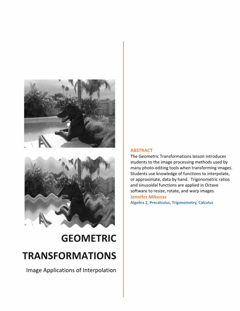
Geometric Transformations - University of Central … · GEOMETRIC TRANSFORMATIONS Image...

GEOMETRIC

TRANSFORMATIONSImage Applications of Interpolation

ABSTRACT The Geometric Transformations lesson introduces students to the image processing methods used by many photo-editing tools when transforming images. Students use knowledge of functions to interpolate, or approximate, data by hand. Trigonometric ratios and sinusoidal functions are applied in Octave software to resize, rotate, and warp images.

Jennifer Mikenas Algebra 2, Precalculus, Trigonometry, Calculus

Contents LESSON OVERVIEW ......................................................................................................................... 1

Associated Unit ........................................................................................................................... 1

Summary ..................................................................................................................................... 1

Engineering Connection .............................................................................................................. 1

Subject Area ................................................................................................................................ 1

Time Required ............................................................................................................................. 1

Grade Level ................................................................................................................................. 2

Standards .................................................................................................................................... 2

Materials ..................................................................................................................................... 2

Keywords ..................................................................................................................................... 2

Instructional Design Framework ................................................................................................. 3

Learning Objectives ..................................................................................................................... 3

Prerequisite Knowledge .............................................................................................................. 3

Vocabulary .................................................................................................................................. 3

LESSON BACKGROUND & CONCEPTS FOR TEACHERS .................................................................... 5

LESSON PROCEDURES ................................................................................................................... 11

Introduction & Motivation ........................................................................................................ 13

Lesson Scaling ........................................................................................................................... 14

LESSON EXTENSIONS ..................................................................................................................... 15

TROUBLESHOOTING TIPS .............................................................................................................. 15

FURTHER INFORMATION .............................................................................................................. 15

ACTIVITY 1: 1D Interpolation By Hand .......................................................................................... 16

ACTIVITY 2: 2D Image Interpolation by Octave for Resizing ......................................................... 22

ACTIVITY 3: Image Rotation Using Trigonometric Ratios ............................................................. 33

ACTIVITY 4: Image Rotation Using Trigonometric Equations ....................................................... 39

ACTIVITY 5: Image Warping Using Sinusoidal Functions .............................................................. 40

ASSESSMENT & EVALUATION ....................................................................................................... 46

ATTACHMENTS .............................................................................................................................. 47

REFERENCES .................................................................................................................................. 47

CREDITS ......................................................................................................................................... 48

Geometric Transformations

MIKENAS/INTERPOLATION/JULY2014 1

LESSON OVERVIEW

Associated Unit Poisson Image Blending

Summary The purpose of this lesson is to expose students to real-world applications of the math they use in class every day, with a focus on digital image processing and geometric transformations. Interpolation, using known data to estimate unknown data, can be applied to one and two dimensional applications, meaning to interpolate in one or two directions. Students will first explore one-dimension interpolation, using properties of functions to interpolate linear or polynomial piecewise relationships by hand. These ideas are extended to two dimensional interpolation using Octave software. Trigonometric ratios and formulas are used to perform geometric transformations such as resizing, rotating, and warping images.

Engineering Connection Engineers must fully understand the concepts of interpolation in order to resize images and enhance clarity. Computer engineers use these principles when designing programs that warp images. Students play the role of engineers as they use trigonometry to perform geometric transformations on images.

Subject Area Algebra, Trigonometry, Pre-Calculus, Calculus

Time Required Lesson Introduction: 45 minutes

Octave Introduction: 45 minutes

Module 1: 90 minuteso Activity 1: 45 minuteso Activity 2: 45 minutes

Module 2: 90 minuteso Activity 3: 45 minuteso Activity 4: 45 minutes

Module 3: 45 minuteso Activity 5: 45 minutes

Assessment: 45 minutes For more detailed timelines and suggestions on implementation, please see “Lesson Procedure”

and “Lesson Scaling”.



Grade Level 9th grade – 11th grade

Standards

Common Core Standards for Mathematics, 2014: CCSS Mathematics Florida Standards: MAFS

CCSS.Math.Content.HSF.TF.B.5, MAFS.912.F-TF.2.5: Choose trigonometric functions to model periodic phenomena with specified amplitude, frequency, and midline

CCSS.Math.Content.HSG.SRT.C.8, MAFS.912.G-SRT.3.8: Use trigonometric ratios and the Pythagorean Theorem to solve right triangles in applied problems.

CCSS.Math.Content.HSF.TF.C.9, MAFS.912.F-TF.3.9: Prove the addition and subtraction, half-angle, and double-angle formulas for sine, cosine, and tangent and use these formulas to solve problems.

CCSS.Math.Content.HSF.BF.B.3, MAFS.912.F-BF.2.3. Identify the effect on the graph of replacing 𝑓(𝑥) by 𝑓(𝑥) + 𝑘, 𝑘 𝑓(𝑥), 𝑓(𝑘𝑥), and 𝑓(𝑥 + 𝑘) for specific values of k (both positive and negative); find the value of k given the graphs. Experiment with cases and illustrate an explanation of the effects on the graph using technology.

Materials Student needs:

Activity 1, 2, 3, 4, 5 Worksheets

Computer with Octave software (students may work in pairs on a computer)

Octave files: ‘Resizing.m’, ‘Rotation.m’, ‘Warping.m’ ‘InterpolationComparison.m’

Image file: ‘Otis1.jpg’

Image from student as .jpg file

Keywords amplitude, continuous, cosine, discrete, frequency, interpolation, linear, Octave, period, piecewise, quadratic, rate of change, rotation, sine, transformation, trigonometry

http://www.corestandards.org/Math/Content/HSF/TF/B/5/

http://www.cpalms.org/Public/PreviewStandard/Preview/5593

http://www.corestandards.org/Math/Content/HSG/SRT/C/8/


http://www.corestandards.org/Math/Content/HSF/TF/C/9/




Instructional Design Framework Direct Instruction, Cooperative Learning, Guided Inquiry

Learning Objectives After this lesson, students should be able to:

Write an interpolated piecewise function to represent a discrete sampling of data.

Use trigonometric ratios and formulas to rotate images.

Describe the effect of changing parameters of a sinusoidal function including frequency,

amplitude, and period.

Use technology to resize, rotate, and warp images.

Prerequisite Knowledge Students should be familiar with writing equations of piecewise and linear functions. Students

should be familiar with trigonometric ratios, sine and cosine addition/subtraction formulas, and

graphs of trigonometric functions.

Vocabulary

amplitude The distance from the midline of a periodic function to its maximum or minimum

continuous data Data or a function representing data that may take on an infinite number of values on an interval.

bilinear interpolation An interpolation technique that uses the four nearest neighbors to approximate intensity (Gonzalez & Woods, 2008)

bicubic interpolation An interpolation technique that uses the sixteen nearest neighbors to approximate intensity (Gonzalez & Woods, 2008)

discrete Data that takes on a finite number of values on an interval.

frequency Number of periods per unit of time.

geometric transformation The process of changing the spatial location of pixels in an

image (Gonzalez & Woods, 2008)

image processing The processing of an image as a signal.

interpolation The process of approximating unknown values in between

known values.

linear interpolation An interpolation technique using linear functions to

approximate data.



nearest-neighbor interpolation An interpolation technique that approximates an intensity

by rounding or using the closest value based on proximity.

period The length of time that represents one complete cycle of a periodic function.

translation A horizontal or vertical shift/slide of a function or an image.

warping An image transformation



LESSON BACKGROUND & CONCEPTS FOR TEACHERS

INTRODUCTION BACKGROUND:

Digital vs. Analog

In order to understand interpolation for the purpose of manipulating images, we must first compare analog and digital technology. Analog information is continuous and its signal can be represented by a sine wave with a continuous and infinite set of data values, for example a person’s voice. Digital information is discontinuous and its signals are represented by discrete numerical values, such as a dvd. If digital signals are recorded or sampled using a limited set of values this means there are gaps of unknown data, whereas analog information is continuous. This implies that analog is clearly a more accurate representation of information, so why is technology transitioning to digital? The quality of analog signals can erode over time when transmitted and/or copied (cassettes) whereas digital representation in numeric form is unchanging and therefore will retain its quality. A strong advantage to digitally recorded numeric values is the ability to modify information for various purposes, as you will see in this lesson. By sampling in smaller increments, we can create more accurate representation of a signal. Sometimes we still need information about what is occurring between these discrete values, and that is the reason why interpolation can be so powerful. The main focus of this lesson is to explore various interpolating methods. (Analog vs. Digital, 2014)

Digital Images

When a digital image is created on a camera, your camera is actually registering the amount of light that is reflected off an object, as an intensity value. This intensity is recorded as a numeric value; this recording occurs for every location on the image. These tiny dots of intensity values are pixels (or picture elements) and a digital camera registers that intensity value for three different color channels: red, green and blue. In fact, all colors can be represented by some combination of red, green and blue intensity values. While the digital representation of this image is a single matrix (or three matrices for a colored image) filled with numeric intensity values, these values map a collection of tiny colored dots which appears as the image. Images are stored as a matrix of dimensions 𝑚 × 𝑛. 𝑥 and 𝑦 are directions to a particular pixel location on the image. The numeric values (between 0 and 255) recorded in each position indicate the intensity of the gray for that pixel. 0 represents black; 255 represents white; all values between 0 and 255 represent shades of gray. Color images are actually represented by three different color matrices/channels: red, green, and blue.



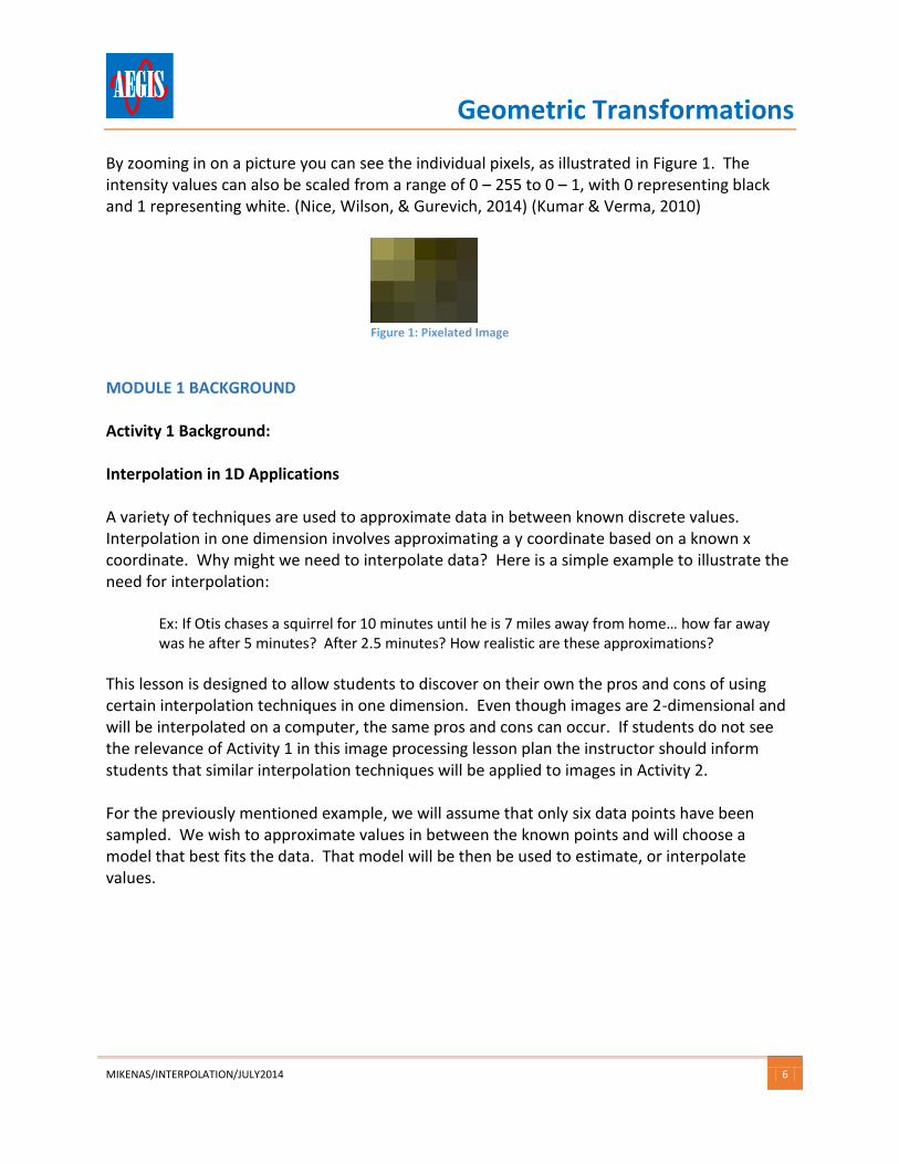
By zooming in on a picture you can see the individual pixels, as illustrated in Figure 1. The intensity values can also be scaled from a range of 0 – 255 to 0 – 1, with 0 representing black and 1 representing white. (Nice, Wilson, & Gurevich, 2014) (Kumar & Verma, 2010)

Figure 1: Pixelated Image

MODULE 1 BACKGROUND

Activity 1 Background:

Interpolation in 1D Applications

A variety of techniques are used to approximate data in between known discrete values. Interpolation in one dimension involves approximating a y coordinate based on a known x coordinate. Why might we need to interpolate data? Here is a simple example to illustrate the need for interpolation:

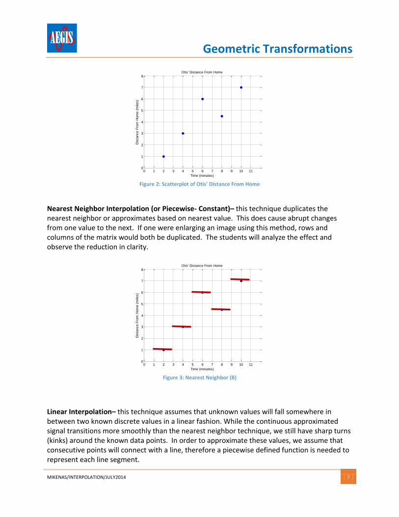
Ex: If Otis chases a squirrel for 10 minutes until he is 7 miles away from home… how far away was he after 5 minutes? After 2.5 minutes? How realistic are these approximations?

This lesson is designed to allow students to discover on their own the pros and cons of using certain interpolation techniques in one dimension. Even though images are 2-dimensional and will be interpolated on a computer, the same pros and cons can occur. If students do not see the relevance of Activity 1 in this image processing lesson plan the instructor should inform students that similar interpolation techniques will be applied to images in Activity 2.

For the previously mentioned example, we will assume that only six data points have been sampled. We wish to approximate values in between the known points and will choose a model that best fits the data. That model will be then be used to estimate, or interpolate values.



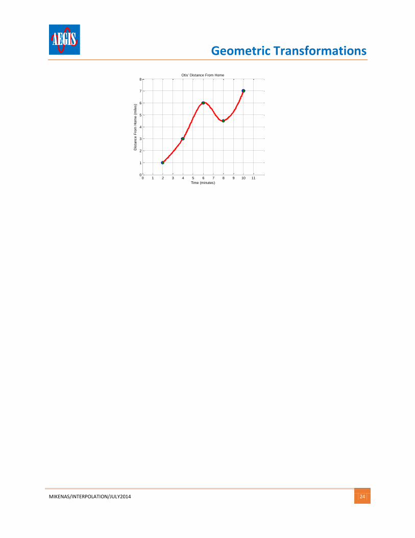
Figure 2: Scatterplot of Otis' Distance From Home

Nearest Neighbor Interpolation (or Piecewise- Constant)– this technique duplicates the nearest neighbor or approximates based on nearest value. This does cause abrupt changes from one value to the next. If one were enlarging an image using this method, rows and columns of the matrix would both be duplicated. The students will analyze the effect and observe the reduction in clarity.

Figure 3: Nearest Neighbor (B)

Linear Interpolation– this technique assumes that unknown values will fall somewhere in between two known discrete values in a linear fashion. While the continuous approximated signal transitions more smoothly than the nearest neighbor technique, we still have sharp turns (kinks) around the known data points. In order to approximate these values, we assume that consecutive points will connect with a line, therefore a piecewise defined function is needed to represent each line segment.

0 1 2 3 4 5 6 7 8 9 10 110

1

2

3

4

5

6

7

8Otis' Distance From Home

Time (minutes)

Dis

tance F

rom

Hom

e (

mile

s)

0 1 2 3 4 5 6 7 8 9 10 110

1

2

3

4

5

6

7


Time (minutes)

Dis

tance F

rom

Hom

e (

mile

s)



Figure 4: Linear Interpolation

Polynomial Interpolation– this technique assumes that unknown data values will fall in between known values (as in the linear method), but approximates as a smooth polynomial function of a higher degree than 1, so that no abrupt changes or sharp turns occur, the figure is continuous and differentiable)

Figure 5: Polynomial Interpolation (Cubic)

Spline Interpolation - this technique uses a piecewise defined function consisting of separate low-degree polynomials for each unknown interval.

0 1 2 3 4 5 6 7 8 9 10 110

1

2

3

4

5

6

7


Time (minutes)

Dis

tance F

rom

Hom

e (

mile

s)

0 1 2 3 4 5 6 7 8 9 10 110

1

2

3

4

5

6

7


Time (minutes)

Dis

tance F

rom

Hom

e (

mile

s)



Figure 6: Spline Interpolation

Activity 2 Background:

Geometric Transformations and Mapping

Geometric Transformations refer to any action on an image that changes the position of pixels, as opposed to an action that might change a color value or intensity of a pixel (Wang, 2013). Anytime a pixel is relocated it may no longer be sitting on a discrete sample position, which means its intensity will need to be approximated, or interpolated. In Activity 2 the students will explore the effect of interpolation on a small number of pixels.

Interpolation in 2D Applications: Geometric Transformations

Two dimensional interpolation is necessary whenever a geometric transformation is performed on an image and requires that two coordinates of a point must be interpolated. Transformations involve modifying the positions of pixels on an image and are useful when resizing, rotating, and warping an image. Note that intensity values of the pixels are not changing. We can use methods similar to those used in 1D applications, with the exception that the technique must be applied along the rows and columns of an image. Since an image may include millions of pixels, we rely on computers to interpolate for us. Nearest-neighbor, bilinear interpolation, and bicubic interpolation are common techniques used on images (the prefix “bi-“ implies that its application is two dimensional).

0 1 2 3 4 5 6 7 8 9 10 110

1

2

3

4

5

6

7


Time (minutes)

Dis

tance F

rom

Hom

e (

mile

s)



Resizing Using Nearest Neighbor: If an image that we wish to double in size contained only four pixels as illustrated in the 2x2 matrix below, the nearest neighbor technique would duplicate the rows and columns. The 4 x 4 matrix illustrates that each row was duplicated once, and then each column was duplicated once. This effect on an image would in fact create four of each single pixel. What effect would this have on an image? While the image has now increased in size, this could create a visible block-like appearance depending on the scale factor used to create the enlarged image (see Powerpoint Slides). Activity 1 focuses on Resizing images.

[7 89 10

]

[

7 7 8 87 7 8 89 9 10 109 9 10 10

]

Other Interpolation Techniques: Bilinear interpolation, in which the nearest four neighbors are used to interpolate an intensity value, involves solving a system of four equations and four unknowns. Similarly, a bicubic interpolation in which the nearest 16 neighbors are used to interpolate an intensity value, involves solving a system of 16 equations and 16 unknowns. MODULE 2 BACKGROUND Rotations: One method of rotating an image is to write a function, or set of directions, that maps each pixel to a new location (intensity values remain the same). Performing this mapping by hand is not a reasonable task, of course, since images may contain millions of pixels so we will rely on computer programs to do this. We can, however, use our knowledge of trigonometric relationships, identities and proofs to create the function which rotates each individual pixel. After rotating a pixel it may no longer sit on a discrete sample, which is why interpolation becomes necessary. Activities 3 & 4 focus on rotating images. Many more interpolation techniques exist. For a more thorough exploration see the University of Illinois lecture notes referenced in the Further Information section of the lesson plan. (Heath, 2002)

Figure 7: Enlarged Image by Nearest Neighbor



MODULE 3 BACKGROUND

Warping: When an image is warped, original pixels are mapped to new locations resulting in distorted features on the image. It is used for distorting images, un-distorting images, or morphing images. This mapping occurs based on a certain transformation designated by a function such as a sinusoid, embedded within the Octave computer program. After warping a point, the pixel may no longer sit on a discrete sample, which is why interpolation becomes necessary. Activity 5 focuses on warping images using properties of sinusoidal functions.

Many more Geometric Transformations exist. For a more thorough exploration see the Polytechnic University lecture notes referenced in the Further Information section of the lesson plan. (Wang, 2013)

LESSON PROCEDURES Before the lesson

o Reserve lab time

o Request Octave installation in reserved labs and on your computer.

o Make copies of students worksheets for Activities 1-5

o Ensure all students have accounts for log-in and access to storing a file on the

server.

o Practice Octave on teacher computer in case technical issues occur in lab and

demo is required.

During the lessono Introduction

Start lesson with “Introduction & Motivation”. Use Powerpoint Section

“Introduction”. Use “Lesson Background and Concepts” for instructional

support during class discussions.

Why are we going digital? Discuss digital vs. analog differences

and need for interpolation

How does a digital camera work? Discuss matrix use for images

What can we do with images? Discuss editing options and

difference between location vs intensity changes

How can images be edited? Introduce Octave in classroom

Octave introduction and practice for Plan A and B implementation only.Use Octave reference materials and practice worksheets.



o Module 1: Interpolation Using Functions

From discrete data students approximate continuous functions including

piecewise-constant, linear and polynomial models and use that to estimate

unknown values. Use Powerpoint Section “Module 1”.

Activity 1 1D Interpolation by hand: Show Interpolation powerpoint slides and use Activity 1 student worksheets. Possible bell-ringer review of writing equation of a line or writing a piecewise function.

Activity 2 2D Image Interpolation by Octave for Resizing: Use Activity 2 student worksheets.

o Module 2: Geometric Transformations using Trigonometry

Students set up dimensions of rotated image using trig ratios. Students write

equations to rotate an image using trigonometric identities. Octave is used to

rotate the image and interpolate the function. Use Powerpoint Section

“Module 2”.

Activity 3 Rotation Using Trigonometric Equations: Show Rotation powerpoint slides and use Activity 3 student worksheets to write rotation equations and rotate images in Octave software.

Activity 4 Rotation Using Trigonometric Ratios: Use Activity 4 student worksheets and octave software to predict and verify dimensions of rotated images and matrices. Possible bell-ringer for solving a right triangle or proving an identity.

o Module 3: Image Warping Using Sinusoids

Students analyze the effects of a sinusoidal warp on an image. Use powerpoint

section “Module 3”.

Activity 5 Octave Image Warping: Show Warping powerpoint slides and use Activity 5 student worksheets.

After the lesson

o Optional Assessment Project. Use Powerpoint Section “Assessment”. o Students complete project and present to the class. o Class discussion on what was learned and wrap up open-ended issues



Introduction & Motivation

1. What does it mean when we use the term “digital”? When our cable company tells us

we must purchase a digital converter for our analog televisions, what are they talking

about? Does anyone know the difference between analog and digital? Why is digital so

much better? (Make list with students and possibly show powerpoint slide “Why Are

We Going Digital?”)

2. Have you ever shopped for a new camera or camera phone and compared the

“megapixels”? Have you ever sent a photo to your friend and been prompted by your

phone to choose what size image you’d like to send? What does this mean? When you

take a photo with a camera and send it to your computer does anyone understand how

this happens? (Show slide on “How does a digital camera work?)

3. Let’s make a list of what kinds of things we can do to an image? (make a list on the

board as students give suggestions):

resize enlarge/shrink

rotate

crop

warp

reflect

morph/blend

brighten

darken

modify contrast

sharpen

Some of these change location of pixels, some change the intensity of color. Can we

classify the items in our list? What do you use to change your images? Sample answers:

Adobe Photoshop, ios or droid apps? (Show powerpoint slide “What can we do with

digital images”. Possibly have students modify an image and demo to class.)

4. How are Images Edited? Have you ever tried to enlarge an image on your computer or

make it smaller to fit in a photo collage? Have you ever tried rotating an image so you

could display it in a document? Or even crop an image to cut out your ex-boyfriend or a

photo-bomber? How exactly does this happen in your software or app? (Show

powerpoint slide “What is MATLAB/OCTAVE?”



Classroom Relevance for Teachers (Course/Topics Covered)

Algebra and Algebra 2 instructors can incorporate 1-dimensional interpolation and 2-dimensional image resizing into their lessons as a means of illustrating linear and quadratic relationships by writing piecewise defined functions. Precalculus and Trigonometry instructors can incorporate 2-dimensional interpolation and geometric transformation of images into their lessons as a means of illustrating trigonometric relationships, trigonometric formulas, and application of proofs. Trigonometric formulas will be used to prove rotation formulas that are used in computer programs for the rotation of images. Students will analyze the visual impact of warping an angle by changing the parameters of a sinusoidal function.

Lesson Scaling

Implementation and Student Level Scaling o Plan A (Full implementation): Student access to lab for seven days. Full

implementation of all three modules, all five activities, and Octave

introduction. Students work in lab for entire lesson. During class, students

work independently on activity worksheets and instructor circulates to field

questions. Best suited for honors students.

o Plan B (Mid-weight implementation): Student access to lab for 2-4 days.

Implementation of all three modules and all five activities, with Octave

introduction. Some Octave activities are demonstrated by instructor only

based on timing of lab access. During classroom days, instructor

demonstrates octave program followed by class discussion. During lab time,

students work independently or in pairs.

o Plan C (Light implementation): No lab access required. All three modules

and five activities are implemented. Distribute student worksheets for each

activity, but all octave portions of the activities are demonstrated by the

instructor followed by class discussion and/or partner discussion.



LESSON EXTENSIONS Students can research other types of geometric transformations that are performed on images,

and the mathematic concepts associated with these transformations. Students can research

careers that involve interpolation, in the image processing industry and out of the industry.

Students can research other geometric mapping models including Chirping and Non-Chirping

Models, Swirling effects, image registration. The Polytechnic University Lecture on Geometric

Transformations is a great launching point for students.

TROUBLESHOOTING TIPS [(optional) Anticipated problems - Think through likely common snags that might be

encountered while conducting the lesson and activity. Suggest solutions, approaches to avoid

pitfalls, etc. This section may be easier to complete after implementation.]

FURTHER INFORMATION

Geometric Transformations: http://eeweb.poly.edu/~yao/EL5123/lecture12_ImageWarping.pdf

is a Polytechnic University Lecture presentation on Geometric Transformations including

Warping, Registration, and Morphing with a thorough explanation on forward mapping and

inverse mapping. (Wang, 2013)

Interpolation: http://web.engr.illinois.edu/~heath/scicomp/notes/chap07.pdf is an excellent resource from the university of Illinois on more advanced interpolation methods including polynomial, piecewise-polynomials (spline), Newton, and Lagrange. (Heath, 2002)

http://eeweb.poly.edu/~yao/EL5123/lecture12_ImageWarping.pdf

http://web.engr.illinois.edu/~heath/scicomp/notes/chap07.pdf



ACTIVITY 1: 1D Interpolation By Hand

Goals / Background Information In this activity we use our knowledge of functions, continuity and rates of change to choose

appropriate interpolation techniques. Recall that interpolation is the act of approximating data

for unknown values based on known values. We will use discrete data to approximate a

continuous model and use this continuous model to approximate unknown data. Why might we

need interpolation? Let’s use a simple example to illustrate the need for interpolation.

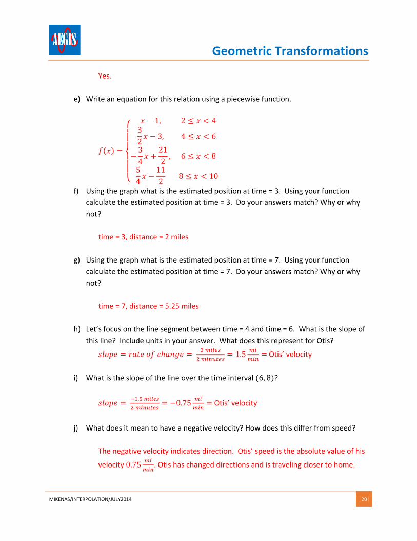
Example: Otis chases a squirrel for 10 minutes until he is 7 miles away from home… how far away was he after 5 minutes?

How accurate is your estimate? What if we wanted to estimate more values? During this activity we will evaluate several interpolation techniques and consider the pros and cons of each. In Activity 2 we will apply these one-dimensional techniques to images, which are two dimensional.

Activity Procedures

Let’s assume that several of Otis’ whereabouts have been recorded by neighbors. Error!

eference source not found. includes Otis’ distance from home at six different times. Follow the

steps below to practice interpolating using several different techniques.

0 1 2 3 4 5 6 7 8 9 10 110

1

2

3

4

5

6

7


Time (minutes)

Dis

tance F

rom

Hom

e (

mile

s)



1) Nearest Neighbor Interpolation Technique

a) This technique assumes that any unknown value will be rounded to the nearest

known value. Under this condition, write the corresponding values:

Time Distance from

Home

2.1 2

2.5 2

3.5 4

4 4

4.7 4

6.8 6

7 8

* a value of 8 assumes that a median rounds up

b) On the figure above, draw in your best estimate of what this graph would look like

for all values of x.

Student graphs may vary.

c) How would you describe this graph? Is it similar to anything else you’ve studied?

Piecewise functions, constant functions, step functions.

0 1 2 3 4 5 6 7 8 9 10 110

1

2

3

4

5

6

7


Time (minutes)

Dis

tance F

rom

Hom

e (

mile

s)

0 1 2 3 4 5 6 7 8 9 10 110

1

2

3

4

5

6

7


Time (minutes)

Dis

tance F

rom

Hom

e (

mile

s)



Let’s explore the characteristics of this technique under the context of Otis taking his daily run.

d) Does your graph represent a function? Why or why not?

Answers will vary depending on student graph.

e) If in fact Otis is chasing a squirrel, should this graph represent a function? Why or

why not?

Yes, his position should represent a function. If the graph is not a function then

Otis would be in two places at once, which is impossible. For example, at t = 3,

Otis could not be 1 mile from home and 3 miles from home.

f) Write an equation for this relation, if it were a function. For consistency, lets

assume that any median values round up to the next known integer.

Piecewise-Defined function of constants 𝑓(𝑥) =

{

2, 1 ≤ 𝑥 < 34, 3 ≤ 𝑥 < 56, 5 ≤ 𝑥 < 78 7 ≤ 𝑥 < 910 9 ≤ 𝑥 < 11

g) If the position were represented by a piecewise function of constants there are

jumps on the graph. Would the graph of Otis’ position need to be continuous?

Yes, it must be a continuous function. Otis cannot immediately jump from a

position of 1 mile to 3 miles.

h) Considering the need for a continuous function, would it make sense to use this

nearest neighbor technique? Why or why not?

No, nearest neighbor in this context would result in jumps from one value to the

next.



i) Why might Otis’ distance from home remain constant between t = 3 and t = 5?

He could have stopped to catch his breath or lick a lizard. He also could be

running in a perfectly circular fashion around his home, in which case the radius

represents the distance from home and remains constant.

j) What would be a more realistic estimate at time = 3 minutes? How did you arrive at

this predicted value?

Students may use lines between known points: distance = 2 mi

Curves between known points: distances may vary

2) Linear Interpolation

a) What if we were to assume that each pair of values were connected with a straight

line segment. Draw in your best estimate of what this graph would look like.

b) How would you describe this graph?

Piecewise-Defined function of Lines

c) Does your graph represent a function? Why or why not?

Yes, for every time value there is no more than one corresponding distance.

d) We have already established the need for Otis’ distance to be represented by a

continuous function. Is this a function? Is it continuous?

0 1 2 3 4 5 6 7 8 9 10 110

1

2

3

4

5

6

7


Time (minutes)

Dis

tance F

rom

Hom

e (

mile

s)



Yes.

e) Write an equation for this relation using a piecewise function.

𝑓(𝑥) =

{

𝑥 − 1, 2 ≤ 𝑥 < 43

2𝑥 − 3, 4 ≤ 𝑥 < 6

−3

4𝑥 +

21

2, 6 ≤ 𝑥 < 8

5

4𝑥 −

11

28 ≤ 𝑥 < 10

f) Using the graph what is the estimated position at time = 3. Using your function

calculate the estimated position at time = 3. Do your answers match? Why or why

not?

time = 3, distance = 2 miles

g) Using the graph what is the estimated position at time = 7. Using your function

calculate the estimated position at time = 7. Do your answers match? Why or why

not?

time = 7, distance = 5.25 miles

h) Let’s focus on the line segment between time = 4 and time = 6. What is the slope of

this line? Include units in your answer. What does this represent for Otis?

𝑠𝑙𝑜𝑝𝑒 = 𝑟𝑎𝑡𝑒 𝑜𝑓 𝑐ℎ𝑎𝑛𝑔𝑒 = 3 𝑚𝑖𝑙𝑒𝑠

2 𝑚𝑖𝑛𝑢𝑡𝑒𝑠= 1.5

𝑚𝑖

𝑚𝑖𝑛= Otis’ velocity

i) What is the slope of the line over the time interval (6, 8)?

𝑠𝑙𝑜𝑝𝑒 = −1.5 𝑚𝑖𝑙𝑒𝑠

2 𝑚𝑖𝑛𝑢𝑡𝑒𝑠= −0.75

𝑚𝑖

𝑚𝑖𝑛= Otis’ velocity

j) What does it mean to have a negative velocity? How does this differ from speed?

The negative velocity indicates direction. Otis’ speed is the absolute value of his

velocity 0.75𝑚𝑖

𝑚𝑖𝑛. Otis has changed directions and is traveling closer to home.



Note to instructor: Other topics to discuss with the class might include

increasing/decreasing functions, domain and range, average rate of change.

k) What is Otis’ speed at the following times

4.5 seconds? 1.5𝑚𝑖

𝑚𝑖𝑛 the slope of the line





Is it realistic that Otis will maintain the same speed throughout the timeframe

between t = 4 and t = 6 minutes?

No, he is not on cruise control. Realistically his speed will constantly change.

l) What is Otis’ speed at the following times


𝑚𝑖𝑛

6.0001 seconds? −0.75𝑚𝑖

𝑚𝑖𝑛=

Is it realistic that in such a small time frame from t = 5.999 to 6.001 seconds his

speed could change so quickly?

No, the transition would occur in a smoother fashion.

m) What is his speed at 6.0 seconds when he is changing direction?

Speed is zero mi/min at 6.0 seconds because he is changing directions.

n) Does the Linear method of interpolation make sense in the context of this story?

No, Otis would not run at such constant speeds with such sharp turns. Note to

instructor: could possibly mention kinks and differentiability.



3) Other Interpolation techniques

a) On the figure below, sketch a more appropriate continuous function that could

be used to interpolate Otis’ distance and describe it.

A function that is represented by a smooth continuous curve, possibly a polynomial.

b) We have explored Nearest Neighbor and Linear Interpolation. Discrete data can

actually be interpolated using many different methods. Several are listed below.

Research the interpolation techniques and briefly summarize each.

Polynomial Interpolation: a single higher degree polynomial is used to represent

the continuous function.

Spline Interpolation: A piecewise functions whose parts are represented by low

degree polynomials

Bilinear: a weighted average technique used in two-dimensional applications

such as image processing in which 4 nearby intensities are considered when

interpolating the image.

Bicubic Interpolation: a weighted average technique used in two-dimensional

applications such as image processing in which 16 nearby intensities are

considered when interpolating the image.

0 1 2 3 4 5 6 7 8 9 10 110

1

2

3

4

5

6

7


Time (minutes)

Dis

tance F

rom

Hom

e (

mile

s)



c) Below is a listing of several other techniques used by MATLAb and Octave

software programs to interpolate one dimensionally.

'nearest' - nearest neighbor interpolation

'linear' - linear, bilinear, trilinear,... interpolation

'spline' - spline interpolation

'pchip' - shape-preserving piecewise cubic interpolation (1D only)

'cubic' - cubic, bicubic, tricubic,... for uniformly spaced data only

0 1 2 3 4 5 6 7 8 9 10 110

1

2

3

4

5

6

7


Time (minutes)

Dis

tance F

rom

Hom

e (

mile

s)

0 1 2 3 4 5 6 7 8 9 10 110

1

2

3

4

5

6

7


Time (minutes)

Dis

tance F

rom

Hom

e (

mile

s)



0 1 2 3 4 5 6 7 8 9 10 110

1

2

3

4

5

6

7


Time (minutes)

Dis

tance F

rom

Hom

e (

mile

s)



ACTIVITY 2: 2D Image Interpolation by Octave for Resizing

Goals / Background Information

Interpolation in 2D Applications: Geometric Transformations Two dimensional interpolation is necessary whenever a geometric transformation is performed on an image. Geometric Transformations involve modifying the positions of pixels on an image and are useful when resizing, rotating, and warping an image. Note that intensity values of the pixels are not changing. We can use methods similar to those used in 1 dimensional applications, with the exception that the technique must be applied along the rows and columns of an image. Since an image may include millions of pixels, we rely on computers to interpolate for us. Nearest-neighbor, bilinear interpolation, and bicubic interpolation are common techniques used on images (note: the prefix “bi-“ implies that its application is two dimensional).

Activity Procedures

Since a digital image is represented by a matrix, interpolating in two dimensions can be very

labor-intense and time consuming. We will first create our own small matrix, and then allow

the computer to interpolate a large image for us.

1) Open Octave and start a new script in your editor. We will start by creating this simple

matrix, which we will call ‘Original’ with 2 rows and 2 columns.

This is what we’ll set up: Original [0 0.50.5 1

]

This is what we type into Octave: Original = [0 0.5; 0.5, 1]

If instructor is demonstrating, then open pre-written script ‘InterpolationComparison.m’

and run the program.

2) Based on what you’ve learned about intensity values of digital images, what do you expect this Original image to look like? To check against your prediction, type a new line:

imshow(Original)

Once you’ve viewed the figure, delete or comment out this imshow line before proceeding.



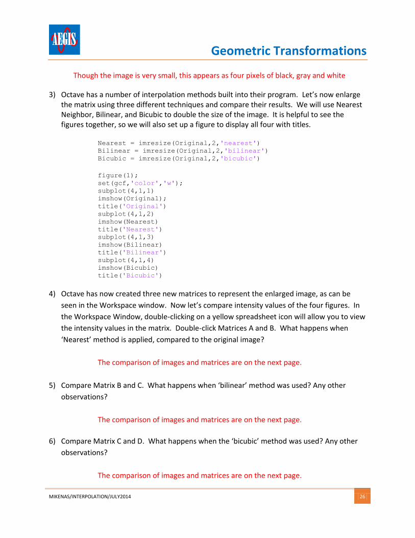
Though the image is very small, this appears as four pixels of black, gray and white

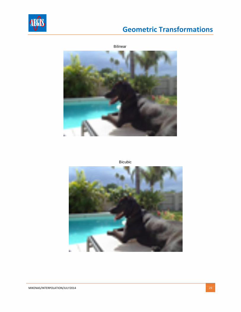
3) Octave has a number of interpolation methods built into their program. Let’s now enlarge the matrix using three different techniques and compare their results. We will use Nearest Neighbor, Bilinear, and Bicubic to double the size of the image. It is helpful to see the figures together, so we will also set up a figure to display all four with titles.

Nearest = imresize(Original,2,'nearest') Bilinear = imresize(Original,2,'bilinear') Bicubic = imresize(Original,2,'bicubic')

figure(1); set(gcf,'color','w'); subplot(4,1,1) imshow(Original); title('Original') subplot(4,1,2) imshow(Nearest) title('Nearest') subplot(4,1,3) imshow(Bilinear) title('Bilinear') subplot(4,1,4) imshow(Bicubic) title('Bicubic')

4) Octave has now created three new matrices to represent the enlarged image, as can be

seen in the Workspace window. Now let’s compare intensity values of the four figures. In

the Workspace Window, double-clicking on a yellow spreadsheet icon will allow you to view

the intensity values in the matrix. Double-click Matrices A and B. What happens when

‘Nearest’ method is applied, compared to the original image?

The comparison of images and matrices are on the next page.

5) Compare Matrix B and C. What happens when ‘bilinear’ method was used? Any other

observations?


6) Compare Matrix C and D. What happens when the ‘bicubic’ method was used? Any other

observations?




Original Matrix

’Nearest Neighbor’ method:

rows and columns have been

duplicated. image has

doubled, but has same

appearance with four

separate squares

‘Bilinear’ method: linear

growth, consistent rate of

change from first intensity to

the last. ON image, colors

gradually increase from

black, to gray to white.

‘Bicubic’ method: values

start below the lowest

intensity value, and exceed

the highest value, with

smoother transitions through

gray.

Original

Nearest

Bilinear

Bicubic



7) Now let’s resize an existing image and compare the same interpolation techniques. Open

Resizing.m and run the program. The Figures will be sitting on top of each other so you will

need to reposition the figures for comparison.

a) Compare your Original image in Figure 1 to the Nearest image in Figure 2. What is

the first thing you notice about Nearest technique? Is that what you expected?

Significant loss of clarity of the image.

b) How would you compare Nearest to Bilinear and Bicubic?

Nearest has a square block-like appearance since intensity values are getting

repeated. Bilinear is more clear than the Neighbor technique. Bicubic seems to

have the greatest clarity. See the figure below.

Nearest



Bilinear

Bicubic



Activity (Title) Answer Key [Provide an answer key for all projects, worksheets, etc. Embedded within the document.]



ACTIVITY 2 OCTAVE CODE: InterpolationComparison.m

File contents:

clc clear close all

Original = [0 0.5; 0.5, 1] %creates Orginal 2x2 matrix

Nearest = imresize(Original,2,'nearest') % nearest neighbor interpolation

(scale of 2)

Bilinear = imresize(Original,2,'bilinear') % bilinear interpolation (scale of

2)

Bicubic = imresize(Original,2,'bicubic') % bicubic interpolation (scale of 2)

figure(1); set(gcf,'color','w'); subplot(4,1,1) imshow(Original); title('Original') subplot(4,1,2) imshow(Nearest) title('Nearest') subplot(4,1,3) imshow(Bilinear) title('Bilinear') subplot(4,1,4) imshow(Bicubic) title('Bicubic')



ACTIVITY 2 OCTAVE CODE: Resizing.m

File contents:

%imresizing image with different techniques clc close all clear

Original = imread('Otis1.jpg'); imshow(Original) title('Original')

%% resizes original image halfsize B = imresize(Original,0.08); figure(1) imshow(B) title('Original')

%% shows halfsize by nearest neighbor Nearest = imresize(B,5, 'nearest'); figure (3) imshow (Nearest) title('Nearest')

%% shows halfsize by bilinear Bilinear = imresize(B,5, 'bilinear'); figure (4) imshow (Bilinear) title('Bilinear')

%% shows halfsize by bicubic Bicubic = imresize(B,5, 'bicubic'); figure (5) imshow (Bicubic) title('Bicubic')

%% Plots three methods side by side, but images are small % figure(2) % set(gcf,'color','w'); % title('Original') % subplot(1,3,1) % imshow(Nearest) % title('Nearest') % subplot(1,3,2) % imshow(Bilinear) % title('Bilinear') % subplot(1,3,3) % imshow(Bicubic) % title('Bicubic')



(x,y)

x

y

(u,v)

α

θ

u

v

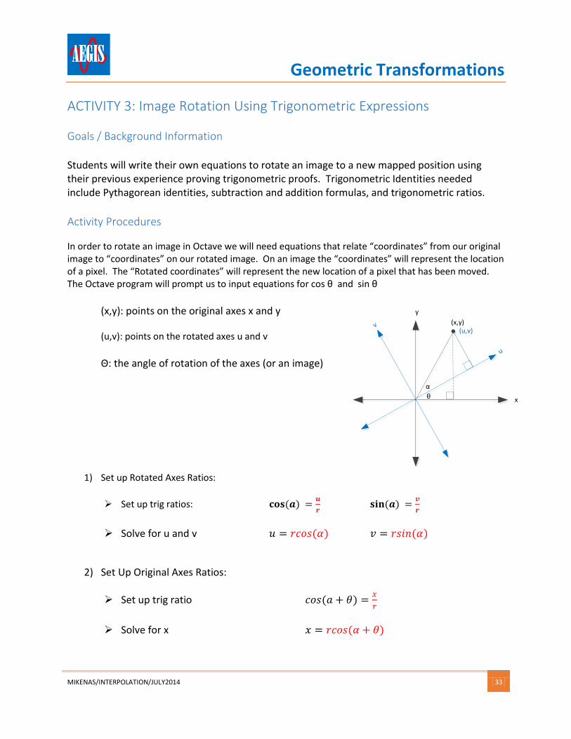
ACTIVITY 3: Image Rotation Using Trigonometric Expressions

Goals / Background Information Students will write their own equations to rotate an image to a new mapped position using their previous experience proving trigonometric proofs. Trigonometric Identities needed include Pythagorean identities, subtraction and addition formulas, and trigonometric ratios.

Activity Procedures

In order to rotate an image in Octave we will need equations that relate “coordinates” from our original image to “coordinates” on our rotated image. On an image the “coordinates” will represent the location of a pixel. The “Rotated coordinates” will represent the new location of a pixel that has been moved. The Octave program will prompt us to input equations for cos θ and sin θ

(x,y): points on the original axes x and y (u,v): points on the rotated axes u and v

Θ: the angle of rotation of the axes (or an image)

1) Set up Rotated Axes Ratios:

Set up trig ratios: 𝐜𝐨𝐬 (𝒂) =𝒖

𝒓 𝐬𝐢𝐧 (𝒂) =

𝒗

𝒓

Solve for u and v 𝑢 = 𝑟𝑐𝑜𝑠(𝛼) 𝑣 = 𝑟𝑠𝑖𝑛(𝛼)

2) Set Up Original Axes Ratios:

Set up trig ratio 𝑐𝑜𝑠 (𝑎 + 𝜃) =𝑥

𝑟

Solve for x 𝑥 = 𝑟𝑐𝑜𝑠(𝛼 + 𝜃)



3) Use trigonometric formulas to write 𝑥 in terms of 𝑢 , 𝑣 , and Note to instructor: Hints on the left are optional. Delete hints if students are capable.

Start with x equation 𝑥 = 𝑟𝑐𝑜𝑠(𝛼 + 𝜃)

Expand using cosine addition formula 𝑥 = 𝑟[cos(𝑎) cos(𝜃) − sin(a) sin (θ)]

Distribute r 𝑥 = rcos(a) cos(θ) − rs𝑖𝑛(𝑎)sin (𝜃)

Substitute with u and v 𝑥 = 𝑢𝑐𝑜𝑠(𝜃) − 𝑣𝑠𝑖𝑛(𝜃)

4) Write 𝑦 in terms of 𝑢 , 𝑣 , and

Note to instructor: Hints on the left are optional. Delete hints if students are capable.

Set up trig ratio 𝑠𝑖𝑛 (𝑎 + 𝜃) =𝑦

𝑟

Solve for x 𝑦 = 𝑟𝑠𝑖𝑛(𝛼 + 𝜃)

Expand using cosine addition formula 𝑦 = 𝑟[𝑠𝑖𝑛(𝑎) 𝑐𝑜𝑠(𝜃) + 𝑐𝑜𝑠(𝑎) 𝑠𝑖𝑛 (𝜃)]

Distribute r 𝑦 = 𝑟𝑠𝑖𝑛(𝑎) 𝑐𝑜𝑠(𝜃) + 𝑟𝑐𝑜𝑠(𝑎)𝑠𝑖𝑛 (𝜃)

Substitute 𝑦 = 𝑣𝑐𝑜𝑠(𝜃) + 𝑢𝑠𝑖𝑛(𝜃)

5) Open the Rotation.m file. When prompted input your rotated equations for both x and y. Be

sure to use ‘ * ‘ for multiplication and ‘theta’ for 𝜽.

Students should input: 𝒙 = 𝒖𝒄𝒐𝒔(𝜽) − 𝒗𝒔𝒊𝒏(𝜽) 𝒚 = 𝒗𝒄𝒐𝒔(𝜽) + 𝒖𝒔𝒊𝒏(𝜽)

6) Did the image rotate? If not, try to decipher the error received by Octave. Check your work.

If the image rotated, continue to Activity 4.

There is a default option written in the program for students who continue to struggle. Have the student run the program again, but when prompted for the equations type nothing and press the enter key.






ACTIVITY 3 & 4 OCTAVE CODE: Rotation.m

File contents BEING WORKED ON BY DR. A, TO BE EMAILED TUESDAY NIGHT, INSERTED WEDNESDAY MORNING



ACTIVITY 4: Image Rotation Using Trigonometric Ratios

Goals / Background Information In this lesson we will use trigonometric ratios and identities to rotate images. You’ve learned that all images can be stored digitally as matrices with dimensions representative of the amount of pixels of the image. When using computer programs to map pixels to new locations, we must frequently start by initializing a matrix and setting up its new dimensions. In this activity we will practice finding the new dimensions of a matrix after an image has been rotated.

Activity Procedures

1) Let’s assume we wish to rotate an image 30°. The original image is a 720 x 960 pixel image. Using your knowledge of trigonometric ratios, find the new width and length of the image, which represents the dimensions of the new matrix within which the rotated image will reside?

720

960

30°

Students can find lengths of the legs of the grey right triangles above and sum to find the width and length.

width = 960𝑠𝑖𝑛30º + 720𝑐𝑜𝑠30º ≈ 1104

length = 720𝑠𝑖𝑛30º + 960𝑐𝑜𝑠30º≈1191

2) In the command window of Octave open the file Rotated.m, if it is not already open, and run the program.

If you have completed Activity 3: when prompted for the rotation angles you may input your own equations. If you have not completed Activity 3: when prompted for equations do not type anything and press Enter.

width

length



3) When prompted for the angle of rotation, choose 30°. Has the image rotated as you

would expect? Check the Workspace window for dimensions of the matrices.

Yes, answer differs slightly due to rounding. Third matrix dimension of 3 is referencing the three color channel matrices: 1: red, 2: green, 3: blue

4) By typing in the command window “whos” OCTAVE will identify all variables and their

dimensions. Check the dimensions of the original image to those of the transformed image.

Insert new Figure based on new code/variables from Dr. A

5) Why are our answers slightly smaller than the true matrix? Hint: consider what you know about how digital images are stored.

Matrices consist of discrete numbers of elements, rows, and columns. If the entire image is to be visible, each of the components of x and y must be rounded up to ensure no portion of the image is cut off.

6) Let’s assume we wish to rotate an image θ°. The image is a 𝑢 x 𝑣 image. What would be

the dimensions of the new matrix, in terms of θ, within which the rotated image will reside?

u

vvv

θ

x

y

𝑤𝑖𝑑𝑡ℎ = 𝑣𝑠𝑖𝑛𝜃 + 𝑢𝑐𝑜𝑠𝜃

𝑙𝑒𝑛𝑔𝑡ℎ = 𝑢𝑠𝑖𝑛θ + 𝑣𝑐𝑜𝑠𝜃



7) Use your equations from Step 5 to determine the matrix dimensions needed for a 45º rotated image.

𝑤𝑖𝑑𝑡ℎ = 960𝑠𝑖𝑛45º + 720𝑐𝑜𝑠45º ≈ 1188 𝑙𝑒𝑛𝑔𝑡ℎ = 720𝑠𝑖𝑛45º + 960𝑐𝑜𝑠45º≈1188

8) Re-run the program with a 45º rotation. Re-run the program and verify.

Dimensions in workspace window are 1189 by 1189. Actual answers differ slightly for reasons mentioned earlier.

9) On Figure 2 the grey section represents the portions of the rotated matrix that do not include a pixel intensity from the original image matrix. On the figure you created in Octave, it does not actually appear as gray but another color. By looking at your figure, what would we expect of the pixel intensity values in this section of the matrix in Octave? Why might this be based on what you’ve previously learned of Octave?

Before an image/matrix is transformed, it is customary for the new matrix to be created or “initialized” and filled with zeros. Its pixels are then mapped to a new location. The area outside the rotated image are filled with zeros and remain as zeros. Since zero corresponds to an intensity value of black, we expect the background to be black. If one wished to change this, we could initialize with a value other than black.

10) Let’s verify this by looking at just the red color channel of both the Original Image and

the Rotate Image. In the command window input:

OriginalRed = OriginalImage(:,:,1); RotatedRed = RotatedImage(:,:,1);

Two new matrices should have appeared in your Workspace window titled “OriginalRed” and “RotatedRed”. Beside each variable is a yellow spreadsheet icon. Double-click this icon to open up the matrix in spreadsheet form. What do you observe? Note the size of the original spreadsheet & the rotated spreadsheet, and their respective intensity values.

Check individual intensity values against their rotated position.

The rotated image empty space is filled with zeros, as expected.



ACTIVITY 5: Image Warping Using Sinusoidal Functions

Goals / Background Information In this lesson we will warp images using trigonometric functions, and analyze the effects of

changing parameters within a sinusoidal function.

Activity Procedures After logging in to your computer, open Octave and begin working at your own pace.

1. Open file “warping.m”

2. When prompted for an image, choose your file to warp or use “Otis1.jpg”

3. Run the file by clicking the green Play/Run button from the script.

4. What happened to the image?

The image has a curved appearance due to each pixel being mapped to a new

location.

Look along the bottom row of the image; what does this resemble?

The graph of a sine or cosine function.

5. On lines 36-38 and Line 84 of the program you will see the following script:

Line 36: A = 20; Line 37: T = 128; Line 38: U = X - A * sin(2 * pi * Y / T);

Line 84: Xmapped = U + A * cos(2 * pi * V / T);

Note: Lines 36-38 are creating location of the pixels of the new image. Line 84 is

mapping the intensity of the image. For now, any changes will be made to line 84 in

order for the effect to be visible in the image (check with Dr. A on the wording of

this)

Try replacing the sine function with cosine. How does this affect your image?



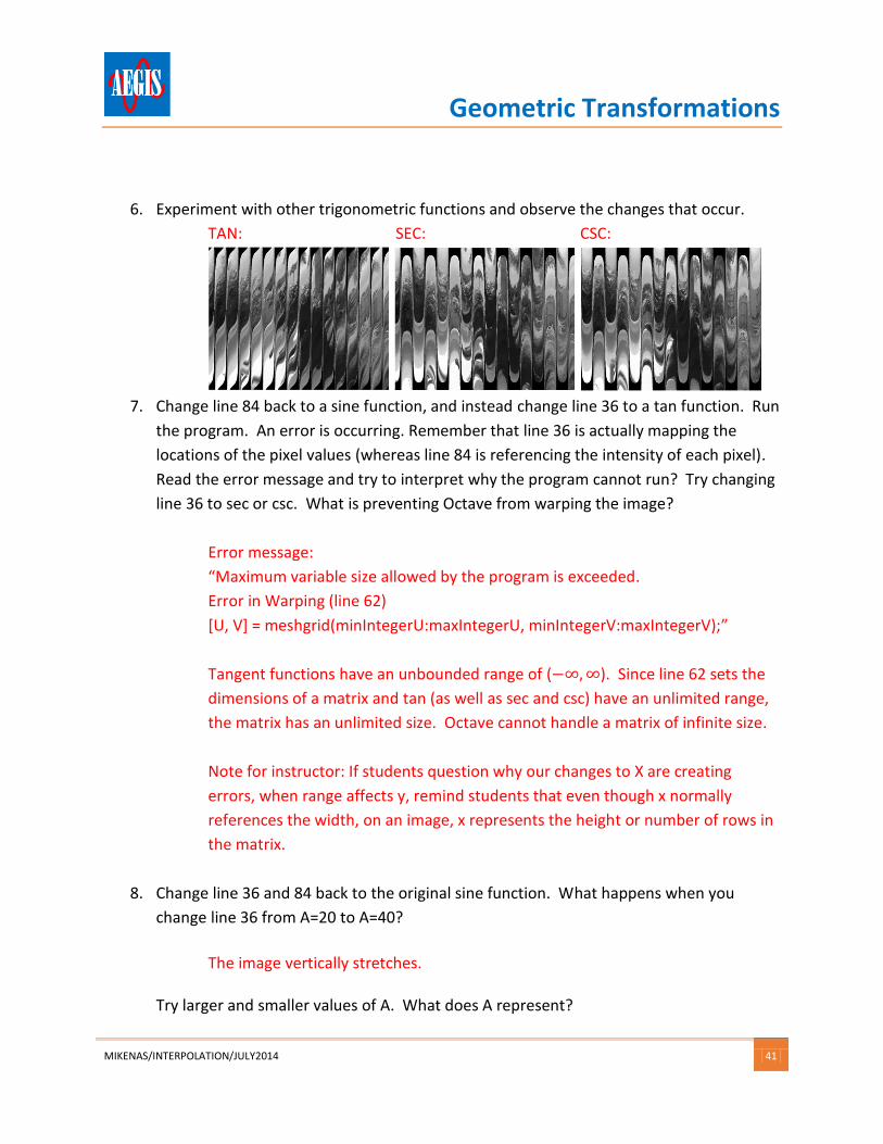
6. Experiment with other trigonometric functions and observe the changes that occur.

TAN: SEC: CSC:

7. Change line 84 back to a sine function, and instead change line 36 to a tan function. Run

the program. An error is occurring. Remember that line 36 is actually mapping the

locations of the pixel values (whereas line 84 is referencing the intensity of each pixel).

Read the error message and try to interpret why the program cannot run? Try changing

line 36 to sec or csc. What is preventing Octave from warping the image?

Error message:

“Maximum variable size allowed by the program is exceeded.

Error in Warping (line 62)

[U, V] = meshgrid(minIntegerU:maxIntegerU, minIntegerV:maxIntegerV);”

Tangent functions have an unbounded range of (−∞,∞). Since line 62 sets the

dimensions of a matrix and tan (as well as sec and csc) have an unlimited range,

the matrix has an unlimited size. Octave cannot handle a matrix of infinite size.

Note for instructor: If students question why our changes to X are creating

errors, when range affects y, remind students that even though x normally

references the width, on an image, x represents the height or number of rows in

the matrix.

8. Change line 36 and 84 back to the original sine function. What happens when you

change line 36 from A=20 to A=40?

The image vertically stretches.

Try larger and smaller values of A. What does A represent?



A represents the amplitude.

9. Using the original sine function and A = 20, re-run the program. What is the value of T

built into the program? What does this represent?

T = 128. T represents the period length.

What might we anticipate if we were to change T? Experiment with other values of T to

see if the expected effect occurs.

The image stretches horizontally.

What would you anticipate happening if you were to use 960? Test your prediction in

the program. What is significant about this value?

960 is the horizontal length of the image. This changes the period length of the

sine curve to the horizontal width of the image. The warped image reflects a

single sine period length only.

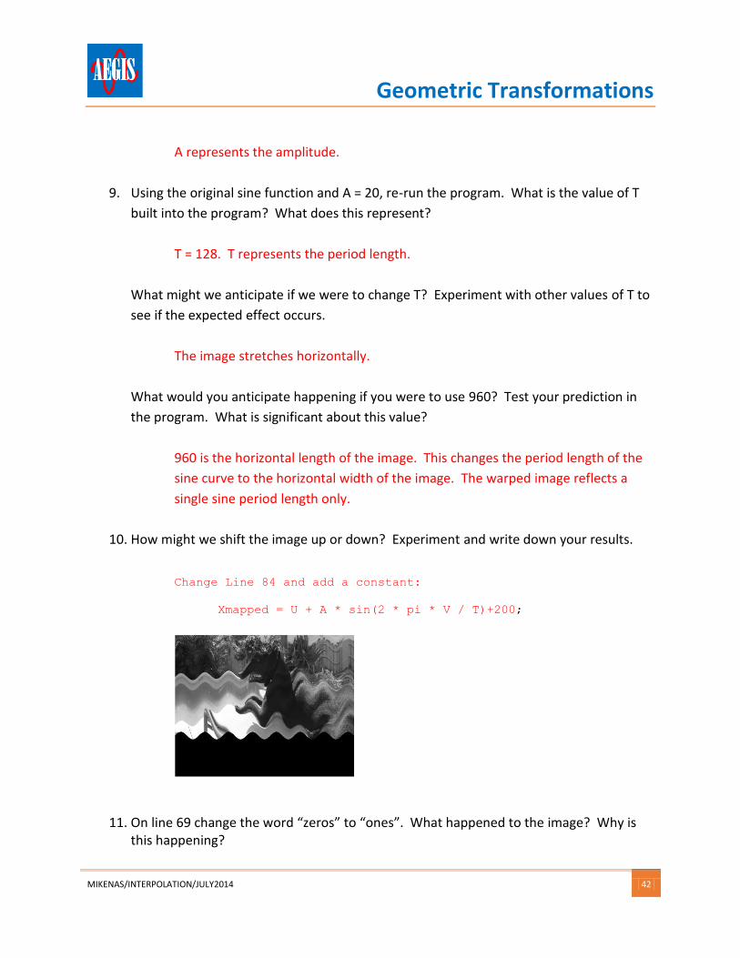
10. How might we shift the image up or down? Experiment and write down your results.

Change Line 84 and add a constant:

Xmapped = U + A * sin(2 * pi * V / T)+200;

11. On line 69 change the word “zeros” to “ones”. What happened to the image? Why is this happening?



The background pixels changed from black to white. An intensity of zero equates to black. An intensity of one equates to white. Line 69 is setting up our initial new image with a matrix filled with intensity values of 1 (instead of zero). All empty space on the new warped image will default to white instead of black.

12. On Line 84 change your equation to the following and note what changes you observe.

Xmapped = U + A * sin(2 * pi * (U) / 100);

Image takes on a rippled wave appearance.

13. Now try modifying other aspects of the equation to see what changes occur. Include

some examples and descriptions below: Equation Effects






ACTIVITY 5 OCTAVE CODE: Warping.m

File contents BEING WORKED ON BY DR. A, TO BE EMAILED TUESDAY NIGHT, INSERTED WEDNESDAY MORNING



ASSESSMENT & EVALUATION

Pre-Lesson Assessment (formative) practice bell ringers to assess students’ prior

knowledge

Activity 1 Bell ringer: Students practice graphing a piecewise function that includes

constant and linear pieces.

𝑓(𝑥) = {3, 𝑥 < −1

2𝑥 − 3, −1 ≤ 𝑥 < 1−𝑥, 1 ≤ 𝑥

Activity 3 Bell ringer: Students practice a trigonometric proof involving sine addition

formula

Activity 4 Bell ringer: Students practice solving a right triangle

Solve the triangle ABC if A = 90°, b = 7, C = 36°

Lesson Embedded Assessment (formative)

After each activity, the student will submit their activity worksheet for participation

points. Worksheet will be handed back (possibly with comments) for the student to

include in their portfolio.

Post-Lesson Assessment (summative):

Students will submit a portfolio including Activities 1-5 and a research report as

described in Lesson Extensions.

Student Feedback Survey:



ATTACHMENTS PowerPoint slides: Interpolation

Octave files: RotationFormula.m, resizing.m, warping.m, Interpolationcomparison.m

Image files: Otis1.jpg

REFERENCES Analog vs. Digital. (2014). Retrieved July 3, 2014, from www.diffen.com. Gonzalez, R. C., & Woods, R. E. (2008). Digital Image Processing 3rd ed. Upper Saddle River:

Pearson. Heath, M. T. (2002). Scientific Computing: An Introductory Survey Ch7 Lecture Notes. Retrieved

July 13, 2014, from University of Illinois Engineering: http://web.engr.illinois.edu/~heath/scicomp/notes/chap07

Kumar, T., & Verma, K. (2010). A Theory Based on Conversion of RGB image to Gray. International Journal of Computer Applications.

Nice, K., Wilson, V. T., & Gurevich, G. (2014). How Ditigal Cameras Work. Retrieved July 3, 2014, from HowStuffWorks.

Wang, Y. (2013). EL5123 /BE6223 Image Processing Lecture 12. Retrieved July 8, 2014, from Polytechnic University: http://eeweb.poly.edu/~yao/EL5123/lecture12_ImageWarping



CREDITS

Authors and Contributors Jennifer Mikenas, teacher, Brevard County Schools Dr. Anagnostopoulos, Associate Professor, Florida Institute of Technology Laura Springstroh, teacher, Brevard County Schools Dr. William Hanna, teacher, Brevard County Schools Jeremy Moore, teacher, Brevard County Schools

Date created / updated Created July 18, 2014.

Supporting Program AEGIS RET Program, College of Engineering and Computer Science, University of Central Florida,

and College of Engineering, Florida Institute of Technology

Acknowledgements This curriculum was developed under National Science Foundation RET grant #1200566 and

#1200552. However, these contents do not necessarily represent the policies of the National

Science Foundation, and you should not assume endorsement by the federal government

Contact information Jennifer Mikenas, [email protected]

[Include your name and email and Dr. A will fill in AEGIS info]

Copyright [TBD - Dr. A fill in ]

mailto:[email protected]

Date post:	28-Aug-2018
Category:	Documents
Upload:	hanguyet
View:	231 times
Download:	0 times

Geometric Transformations - University of Central … · GEOMETRIC TRANSFORMATIONS Image...

Documents