X-592-73-339 PREPRINT GEOMETRICAL GEODESY TECHNIQUES IN GODDARD EARTH MODELS (NASA- M-X-7C619) GEOHEILICAL GEODESY !.74-2098 IECHIQUES IU GCDDALD EAe2H MODELS (NASA) -* p BC $5.00 CSCL 08E 3 Urncias G3/13 36511 F. J. LERCH JANUARY 1974 - -GODDARD SPACE FLIGHT CENTER GREENBELT, MARYLAND Presented at the International Association of Geodesy Symposium on Computational Methods in Geometrical Geodesy, Oxford, United Kingdom, September 2-8, 1973. brought to you by CORE View metadata, citation and similar papers at core.ac.uk provided by NASA Technical Reports Server
(NASA- M-X-7C619) GEOHEILICAL GEODESY !.74-2098IECHIQUES IU GCDDALD EAe2H MODELS (NASA)
-* p BC $5.00 CSCL 08E3 Urncias
G3/13 36511
F. J. LERCH
JANUARY 1974
- -GODDARD SPACE FLIGHT CENTERGREENBELT, MARYLAND
Presented at the International Association of Geodesy Symposium onComputational Methods in Geometrical Geodesy, Oxford, United Kingdom,September 2-8, 1973.
https://ntrs.nasa.gov/search.jsp?R=19740012868 2020-03-23T09:40:55+00:00Zbrought to you by COREView metadata, citation and similar papers at core.ac.uk
The method for combining geometrical data with satellite dy-namical and gravimetry data for the solution of geopotential andstation location parameters is discussed. Geometrical trackingdata (simultaneous events) from the global network of BC-4stations are currently being processed in a solution that willgreatly enhance the geodetic world system of stations. Previ-ously the stations in Goddard Earth Models have been derivedonly from dynamical tracking data. In this paper a linear re-gression model is formulated for combining the data, based uponthe statistical technique of weighted least squares. Reducednormal equations, independent of satellite and instrumental pa-rameters, are derived for the solution of the geodetic parame-ters. Exterior standards for the evaluation of the solution andfor the scale of the earth's figure are discussed.
A matrix model employing a reduced form of the general least squares adjust-ment process is developed. The model provides a method for combining geo-metrical BC-4 optical data with satellite dynamic and gravimetric data into ageneral geodetic solution. The geodetic solution consists of a geocentric systemof station coordinates and spherical harmonic coefficients for the geopotential.A previous solution, Lerch et al (1972), for a Goddard Earth Model (GEM 4) con-tained 514 geodetic parameters but did not include any geometric data.
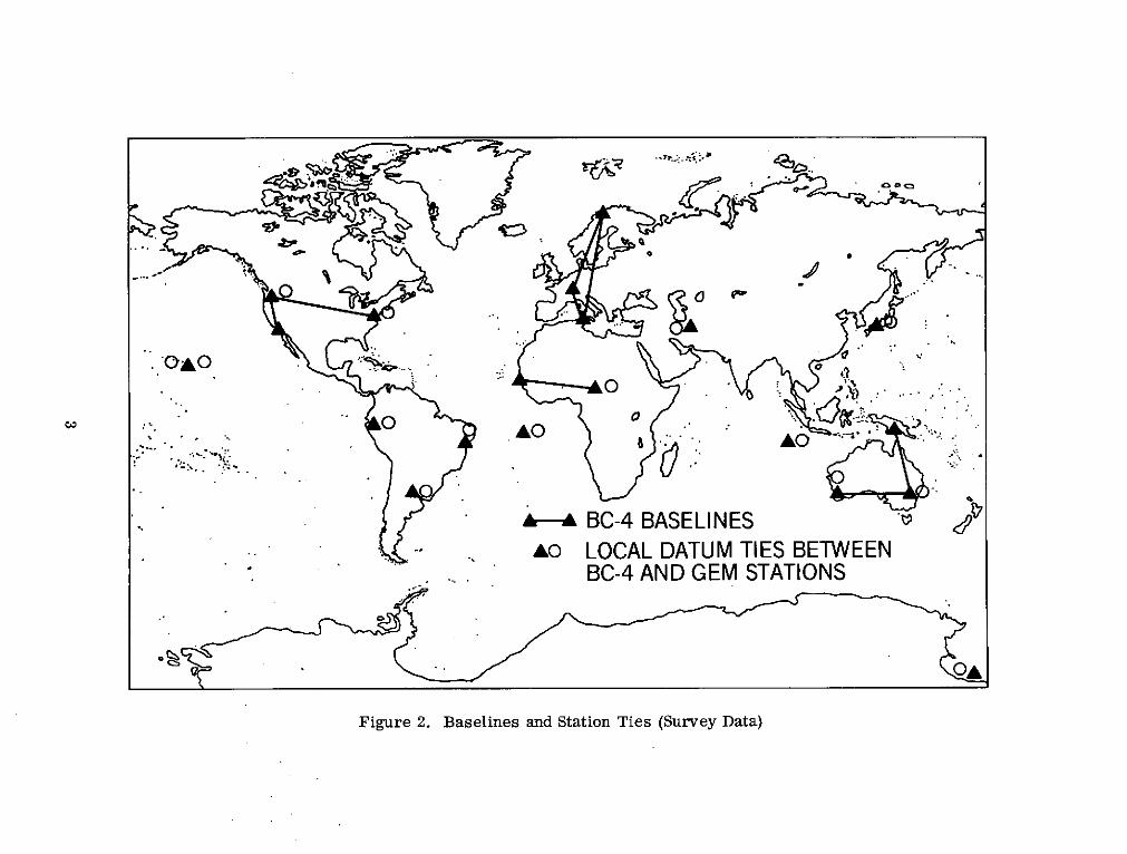
A map of station locations is presented in Figure 1, illustrating the distributionof 45 BC-4 stations associated with the geometric data and 61 stations associatedwith dynamic data from electronic,laser, and optical tracking systems used pre-viously in GEM 4. Figure 2 illustrates local datum ties between the dynamic andgeometric stations and BC-4 baselines obtained from the geodimeter and tellu-rometer systems that are to be employed in the new combination solution.
II. BASIC DATA SYSTEMS AND REPRESENTATION
1. Data Systems
Four basic geodetic data systems are employed in the combination solution andare listed with their associated solution parameters in Table 1. These systemsare the BC-4 geometric (B), gravimetry (G), dynamic satellite (D), and survey (S).
In the survey data system S, the baselines and ties were illustrated in Figure 2.The ties correspond to relative position coordinates for nearby geometrical anddynamical stations and are treated as observations with statistical errors basedupon local survey accuracy. Similarly the baseline distances are treated asstatistical observations.
The satellite related parameters associated with the BC-4 system B and thesatellite dynamic system D require preliminary processing for initial estimatesof the parameters. The initial processing will be discussed in a later section.There are some 20,000 satellite position parameters associated with 1100 BC-4events of two, three, and four stations observing the satellite simultaneously at6 to 7 reduced points of satellite position for each event. There are some 350weekly arcs of satellite dynamic data on 27 satellites, where some 400,000 ob-servations of electronic, laser, and optical tracking data have been processed.
1
o GEM DYNAMIC STATIONS (61)
A BC-4 GEOMETRIC NETWORK (45)
Figure 1. Station Locations
'. oAO o o... ..
CRao
0"O.o ..
v j-.- ,A O . .- A• Ao .. .. :o.,
Ar- BC-4 BASELINES
..- Ao LOCAL DATUM TIES BETWEEN- BC-4 AND GEM STATIONS
i
OA
Figure 2. Baselines and Station Ties (Survey Data)
Table 1Basic Data Systems and Solution Parameters
Solution Parameters UnknownSymbol Data System (unknowns) Symbol
(unknowns) Symbol
B BC-4 geometric station location coordinates xsatellite position componentsfor each geometrical point j qi
G Gravimetry potential coefficients c(spherical harmonic)
D Dynamic satellite potential coefficients cstation coordinates zsatellite orbital elementsand tracking system parametersassociated with each satellitearc i Pi
S Survey station coordinates connecting(Baselines and ties) BC-4 baselines xb in x x
station coordinates connectingties x t in x, z t in z x, z
The satellite dynamic parameters consist of six orbital elements and modeledforce parameters at a given epoch on each weekly arc. Tracking system parame-ters for certain electronic systems have been included in the modeling and areassociated with the initial processing on a weekly are. The gravimetry datasystem G consists of a global distribution of 50 equal area blocks of mean gravityanomalies, Rapp, (1972).
Because of the large number of satellite parameters in the systems B and D, aleast squares matrix model is developed that will reduce the matrix to a formcontaining just the geodetic parameters. The reduced form will then be suitablefor computational solution.
2. Representation of Data Systems
A total data system C, which will be used to encompass the four basic datasystems, is represented as
4
C : (0, C, v; y) (1)
where each symbol denotes a column vector as follows:
O - observations
C - computed quantities corresponding to the observations
v - observation residuals (v = 0 - C)
y - the solution parameters or unknowns (see Table 1)
The column vectors are further defined in Section III where the method for thesolution is developed. The four basic data systems, subsystems of C, are simi-larly represented and defined as in the above form (1), namely
B :(OB,, B, b; x, q) (2)
G : (OG, G, g; c) (3)
S: (OD, Dd; c, z, p) (4)
S : (0s , S, s; z, x) (5)
where the solution parameters c, z, x, p = [pi], q = [q] are defined in Table 1
for each of the data subsystems. Using the form above, data subsystems of Dand B are represented for each dynamic satellite arc i and geometric satellite
position point j, respectively as follows:
Di : (O Di , di; c, z, pi) (6)
Bj : (OBj, Bj, bj; x, q (7)
5
III. DEVELOPMENT OF THE METHOD
1. General Matrix Model for the Least Squares Solution
A general matrix model of the least squares adjustment process is developed for
the complete data system C given in (1). The model will be subsequently employedto develop a reduced form of solution for the geodetic data subsystems.
In the data system C the vector symbols, O, C, v, and the unknown solution y
were defined under (1). The vector C = C (y) and the residual vector is
v = 0 - C(y) (8)
which in component form is
[v n ] = [0, - C (y ) ] for n = 1 to N (9)
where Cn (y) is the computed quantity corresponding to the observation On and is
a function of the parameters in y. The linear condition equation for v in the
least squares adjustment process is given by use of Taylor's expansion as
V = Vo -CyAy , (10)
where v0 = 0 - C (yo), y = y + y, y is a column vector of initial estimates for
each component yk in y for k = 1 to K, and the matrix of partial (derivative) co-efficients
[3 Cn ()(11)
NXK
in which the partial coefficient element lies in row n and column k and Cn (y) isgiven under (9) above. C is evaluated at y = yo.
The least squares minimum condition is
Q = VT W, v = minimum (12)
6
where W is a diagonal weight matrix with each element
1
Wn - for n = 1 to N (13)nn
in which r 2 is the error variance for the observation O . The minimum condi-n n
tion for (12) is obtained from
Y Q= O for k = 1 to K (14)
which with use of (10) and (12) will give the normal equation
C v = O (15)
or
(C ' Wv C) Ay - CT Wv v = 0. (16)
Solving (16) for Ay will give
Ay = (CyTWV C ) C T W v (17)
and the solution y is
Y = Y + Ay.
Under ideal conditions, where the modeling of Cn (y) for On is complete except
for a random observation error which has normal distribution and variance o 2,the least squares solution for y may be shown to satisfy the maximum likelihoodprinciple. See Anderson (1958).
2. Reduced Form of the Normal Equations for the Geodetic Subsystems
Using the column matrices defined for the total data system C under (1) andthose for the geodetic data subsystems in (2) through (5), the following matrixpartitioning is given for C in terms of its data subsystems:
OD D d
0B B bO = C = v = - C = (18)
0G G g
Os S s
Also partition
Fwd C
z AzWbwb
W y = x Ay -y Ax (19)
Wq
where the solution parameters p = [pi], q = [qj] , x z, and c are defined inTable 1, the weight matrix Wv was defined under (13) for C and Wd, Wb, WgW, are defined as diagonal weight matrices respectively for the subsystem ob-servations as ordered in O above. When v and Wv above are substituted into (12),Q then becomes
Q = dT Wd d + b T Wb b + gT Wg g + sT Ws s (20)
In terms of the variables associated with the data subsystem as given in Table 1,the linearized residual equations may be expressed by Taylor's series for eachsubsystem as
8
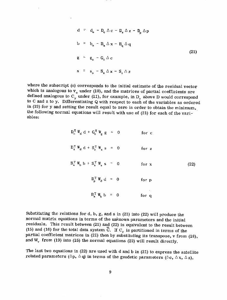
d = do - DcAc - DzA z - DpAp
b = b. - B Ax - Bq q
(21)
g = go - G A c
s = s o - Sx Ax- Sz Az
where the subscript (o) corresponds to the initial estimate of the residual vectorwhich is analogous to v o under (10), and the matrices of partial coefficients aredefined analogous to Cy under (11), for example, in Dz above D would correspondto C and z to y. Differentiating Q with respect to each of the variables as orderedin (19) for y and setting the result equal to zero in order to obtain the minimum,the following normal equations will result with use of (21) for each of the vari-ables:
DTWd d + GT W g = 0 for c
DZ Wd d + ST W s = 0 for z
BT Wb b + ST Ws = 0 for x (22)
DT Wd d = 0 for p
BT Wb b = 0 for q
Substituting the relations for d, b, g, and s in (21) into (22) will produce thenormal matrix equations in terms of the unknown parameters and the initialresiduals. This result between (21) and (22) is equivalent to the result between(15) and (16) for the total data system C. If C, is partitioned in terms of thepartial coefficient matrices in (21) then by substituting its transpose, v from (18),and W, from (19) into (15) the normal equations (22) will result directly.
The last two equations in (22) are used with d and b in (21) to express the satelliterelated parameters (Ap, A q) in terms of the geodetic parameters (Ac, A x, A z).
9
When these results for Ap and Aq are substituted into d and b for the first threeequations of (22), the reduced normal equations will then be obtained for thegeodetic parameters. This process just described is carried out below.
Proceeding in this manner then from (22) and d in (21)
DT Wd d = DT Wd (d o - Dc A c - DZ A z - D Ap) = 0. (23)
Solving (23) for A p and substituting the result back into d will give
d = P(d. - DcAc - D Az) (24)
where
P =I - D P (25)
P = (DTWd D)-I D T Wd (26)
Ap = P(d o - D, Ac - Dz Az) (27)
Proceeding similarly as in (23) with
BT Wb b= 0
then
b = Q (bo - Bx Ax) (28)
where Q and Aq may be derived as in (25) through (27).
By use of d in (24), b in (28), and s and g in (21) the system (22) is expressed inmatrix form for the geodetic parameters as follows:
10
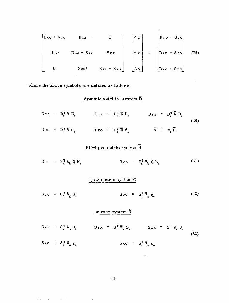
Dcc + Gcc Dcz O Ac Dco + Gco
DczT Dzz + Szz Szx A z = Dzo + Szo (29)
0 SzxT Bxx + Sxx Ax LBxo + SxC
where the above symbols are defined as follows:
dynamic satellite system D
Dcc DTWD Dcz = DTWD Dzz = DTWDz
(30)
Dco DT W d Dzo = DT W do = Wd P
BC-4 geometric system B
Bxx = BT Wb Q Bx Bxo = BT Wb Q bo (31)
gravimetric system G
Gcc = G Wg Gc Gco = GT W go (32)
survey system S
Szz = SW SSzx SZ STW Sx Sxx S= SW, S,
(33)
Szo = STW s s Sxo = STW. S.
11
In the computations the results for D in (30) and B in (31) are expressed in termsof reduced results obtained from the observations on each satellite arc i withsatellite parameters pi and on each satellite geometric point j with coordinatesqj. This situation is represented by the data subsystems Di in (6) and Bj in (7).The data sets and associated partial coefficient matrices of D and B may be par-titioned in terms of these quantities for their respective subsystems to obtain thedetailed results.
The procedure for these results will be briefly derived. From Di in (6) and Din (4)
d i = ODi - Di (c, z, pi) for each i = 1 to I, (34)
d = [di ] D = [Di ] Ap = [Api] p = [ i] (35)
Using Taylor's expansion for d i in (34)
d i = di - Hi A c - Z. Az - pi A Pi (36)
then, from d in (21) and since d = [di],
do = [dio] Dc = [Hi] Dz = [Zi]
(37)
PI o
P2
DP
o PI
Defining the weight matrix Wdi for ODi and ordering it on the diagonal of Wd fori = 1 to I and using the above results for (34) through (37), then (23) through (27)become for each are i
12
P Wdidi = PWdi (dio - Hi Ac - Zi A z - Pi Api) = 0
di = Pi (di - Hi Ac - Zi z)
Pi = I -PiPi (38)
Pi (PT Wdi P)-'P T i
Api Pi (dio - Hi Ac - Zi A z)
and the results in (30) become
Dcc = (HTWiHi) Dcz (HTWZi) Dzz = (ZTWiZi)
(39)
Dco (H Wdi) zo= (I idio) Wi = dii
where the sum ranges from i = 1 to I.
Treating the system B. in (7) in a like manner to Di above, the result in (31)would become
J JBxx = (XT Wi X) Bxo = (X
TWI bio ) , (40)
j=1 j=1
where X. corresponds to Z i, W. to W i, and bj to d..So 10
The solution for the geodetic parameters is obtained through the inverse of thereduced normal matrix in (29). The inverse matrix also represents the variance-covariance matrix for the geodetic parameters, as the weighting for the observa-tions given in (13) is inversely equal to the variance of the observation errors.
13
3. Computational Procedure
In practice the contributions to the reduced normal matrix for each of the geo-
detic subsystems are computed separately and then combined as in (29). The
terms for the reduced normal matrix for each of these four systems are given
separately in equations (30) through (33). The above practice is similarly true
in the computations for the subsystems Di of D and B of B where their respec-
tive matrix terms are identified and combined as in (39) and (40).
The initial starting values for the geodetic parameters are obtained from a pre-
vious geodetic solution, survey data, or through a separate process of data
analysis.
3.1 Satellite Dynamic System
The initial observation residuals and dynamic satellite parameters for the system
Di are obtained from a preliminary reduction of the observation data on a weekly
satellite arc. In this process a bias parameter is modeled for certain electronic
systems for the observation data on each satellite tracking pass. Since a large
number of these parameters may occur within a weekly are span of data, each
bias parameter is eliminated through the back subsitution process at the end of
the associated tracking pass. Numerical integration is employed for the satellite
orbit and the preliminary reduction of the data on the weekly arc is carried out
through the least square process of successive iterations. The normal matrix
for the system Di is formed immediately after the preliminary reduction.
3.2 Geometric Geodesy Technique
In the computations for the BC-4 data system the reduced normal equations (31)
may be obtained through the formulation of condition equations which are inde-
pendent of satellite parameters. This technique is described in the appendix of
the report, and it includes the constraint equations for the station coordinate
ties and baseline distances from datum survey. In addition it provides for use
of simultaneous MOTS and laser data, which has recently been analyzed by
Reece and Marsh (1973) for stations in the area of the United States.
IV. ANALYSIS OF SOLUTION AND GEODETIC RESULTS
The geodetic solution may be tested and analyzed with the use of survey data in
several areas of investigation.
The mean sea level height (MSL) from station survey may be compared with the
height of the station above the geoid as computed from the solution of the poten-
tial coefficients and the geocentric station coordinates including the reference
14
ellipsoid, Lerch et al (1972). In view of the distribution of stations in Figure 1
the dispersion of the differences between survey and computed values about a
mean line may be analyzed. The MSL heights from survey are generally re-
ported to be accurate to about a meter for these stations. Any significant offset
in the mean line from zero differences may be associated with the scale for the
reference ellipsoid, and thus the equatorial radius (ae) of the reference ellipsoidmay be adjusted. Any significant dispersion in the differences (including system-atic differences) may be analyzed in terms of geographical areas and in terms of
various tracking systems such as the electronic, laser, and optical systems.
The dispersion may be analyzed in terms of the geopotential model particularly
in areas where the gravimetric measurements are not available. These analyses
may be supported with separate tests for geoid heights and station coordinates
as indicated below.
Geoid heights computed from the potential model may be tested and analyzed in
certain major survey areas that contain astrogeodetic deflections of the vertical
and detailed gravimetric data, Vincent et al (1972).
Through adjustment for scale, orientation, and datum shift the station coordinates
between datum survey and the solution may be analyzed. In such an analysis fora geocentric station solution by Marsh et al (1971), an rms agreement of 3.5 me-
ters on station coordinate differences has been obtained for 20 stations on the
North American Datum.
With a solution derived from the geodetic data systems and use of the aboveanalysis the following geodetic results may be obtained:
1. A global geoid represented in terms of spherical harmonic coefficients.
2. A world datum of station coordinates including an adjustment for scale,
orientation, and datum shift for local datums.
3. Mean equatorial radius(ae)for the Earth.
4. Mean equatorial value of normal gravity (ge) may be derived from thegravimetric data, Rapp (1972).
15
REFERENCES
1. Anderson, T. W., An Introduction to Multivariate Statistical Analysis,Chapter 2, Wiley, New York, 1958.
2. Lerch, F., Wagner, C., Putney, B., Sandson, M., Brownd, J., Richardson, J.,Taylor, W., "Gravitational Field Models GEM 3 and 4", Goddard Space FlightCenter Document X-592-72-476, November 1972.
3. Lerch, F., Wagner, C., Smith, D., Sandson, M., Brownd, J., Richardson, J.,"Gravitational Field Models for the Earth (GEM 1 & 2)", Goddard SpaceFlight Center Document X-553-72-146, May 1972.
4. Marsh, J. G., Douglas, B. C., Klosko, S. M., "A Unified Set of Tracking Sta-tion Coordinates Derived from Geodetic Satellite Tracking Data", GoddardSpace Flight Center Document X-553-71-370, 1971.
5. Rapp, R. H., "The Formation and Analysis of a 50 Equal Area Block Ter-restrial Gravity Field", Reports of the Department of Geodetic Science No.178, The Ohio State University Research Foundation, Columbus, Ohio, June1972.
6. Reece, J. S., Marsh, J. G., "Simultaneous Observation Solutions For NASA-MOTS and SPEOPT Station Positions on the North American Datum", GoddardSpace Flight Center Document X-592-73-170, June 1973.
7. Vincent, S., Strange, W., Marsh, J., "A Detailed Gravimetric Geoid of NorthAmerica, the North Atlantic, Eurasia, and Australia", Goddard Space FlightCenter Document X-553-72-331, September 1972.
16
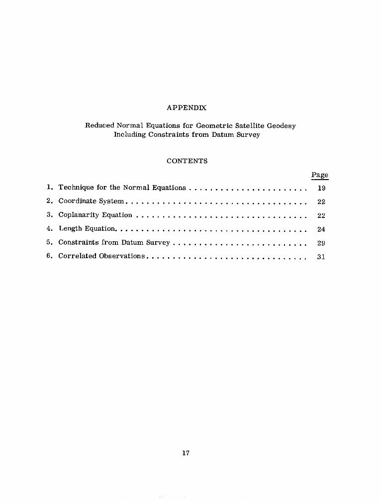
APPENDIX
Reduced Normal Equations for Geometric Satellite GeodesyIncluding Constraints from Datum Survey
CONTENTS
Page
1. Technique for the Normal Equations ....................... 19
2. Coordinate System ................................... 22
Reduced Normal Equations for Geometric Satellite GeodesyIncluding Constraints from Datum Survey
The method developed here for the least squares normal equations is basedupon the technique of formulating reduced condition equations where the satelliteparameters have been eliminated. The data considered consists of simultaneousevents from MOTS (Minitrack Optical Tracking System) and laser systems onGEOS-I and II, the BC-4 worldwide camera network on PAGEOS, and local datumsurvey ties and baselines. The reduced condition equations are developed in this
appendix and a case is considered for the treatment of correlated observations.
1. Technique for the Normal Equations
The mathematical analysis leading to the formation of normal equations forthe geometric adjustment of coordinates of tracking stations is based on the fol-lowing type of events:
1. Two cameras observe the satellite simultaneously2. Three cameras observe the satellite simultaneously3. Four cameras observe the satellite simultaneously4. Two cameras and one laser observe the satellite simultaneously.
Condition equations resulting from a given set of simultaneous observationsare of two types:
* Coplanarity equation, which requires that two observing stations andtheir directions to the satellite lie in the same plane.
* Length equation, which requires that the satellite position satisfying thetwo-station coplanarity relationship also agrees with the range from athird station.
Corresponding to each event condition equations of the following form areused:
m n
Saivi + b bx + c = 0 (1)J
SRM ING PAGE BLANK NOT FILMC19
where a i , b., and c are known constants derived in the subsequent sections,c is the discrepancy in the condition equation
vi are the unknown residuals (adjusted minus observed values)
x. are the unknown corrections to stations' Cartesian coordinates
(adjusted minus initial values)
m is the number of observed quantities
n is the number of unknown coordinates.
The number and types of condition equations for events 1 through 4 above
are as follows:
* For a two-camera event, one coplanarity equation is used.
* For a three-camera event, three coplanarity equations are used.
* For a four-camera event, five coplanarity equations are used.
* For a two-camera, single-laser event, one coplanarity equation and one
length equation are used.
The number of condition equations for each event corresponds to the number of
observations less three, since the observation equations are reduced to a form
where the three satellite position coordinates are eliminated. Each observing
camera contributes two observations in an event and an observing laser contrib-
utes one observation. Each of the coplanarity equations for an event involves
and also take the form of equation (1). Constraints are treated statistically,
similar to observation equations, where values and accuracies are obtained from
a priori information based on datum survey. Two types of constraint equations
are applied:
" Distance equations (baselines), which require the distance between two
stations to remain near a given value
* Coordinate-shift equations, which require the differences between co-
ordinates of two nearby stations to remain near a given value. This
constraint is used to connect the stations in the geometric geodesy with
those in the dynamic satellite geodesy.
For a geometric only solution a third type of statistical constraint may be
applied on individual station coordinates in order to fix the origin of the system.
A priori values for these constraints should be taken from a different source
than datum survey such as from a previously determined geocentric solution in
20
a center of mass reference frame. This constraint is not used in the combina-tion solution with dynamic satellite geodesy.
For each event (or constraint) 4, denote the associated condition equationsof the form (1) in matrix notation as
AVk + B4X + C = 0, (2)
for which an example of the dimensions and elements of the matrices are givenbelow. Minimizing Q below w.r.t. the unknown station coordinates in X andresiduals in VA will lead to the formation of the normal matrix equation. Theform Q is
K
Q = (VW4V4 - 2k(A;V + B&X + C)) (3)
where W~ is the diagonal weight matrix for the observations in VA and eachXA is a column vector of Lagrangian multipliers corresponding to the numberof condition equations in event A. The resulting normal matrix equation to becombined with the gravimetric and dynamic satellite geodesy systems is
K
JX + B MI = N, (4)
where
K
-T = L_ (BM B;),(5)
M (AW'VAT) (6)
The largest dimension of MA is 5 x 5 corresponding to event of type 3 wherethere are 5 coplanarity equations of condition. This case has 8 observations andthe dimensions of AR, Vk, B~, and Ck are respectively 5 x 8, 8 x 1, 5 x Nx , and5 x 1. Nx is the total number of all station coordinates and B (5 x Nx) wouldcontain for each of the 5 rows only 6 non-zero elements, corresponding to theb coefficients in (1) for each distinct coplanarity equation involving two observ-ing stations. Each row of A, has 4 non-zero elements corresponding to the aicoefficients in (1), associated with the two observing stations in each coplanarityequation.
21
By employing a suitable set of constraints including those that fix the origin,
N may be set equal to zero and a geometric only solution for X can be derived
from (4).
Condition equations for coplanarity, length, and constraints are developed
in sections 2 through 5 and section 6 treats a case for correlated observations.
2. Coordinate System
Camera observations in a and 8 are transformed from right ascension a
and declination 8 to earth-fixed angles 8 and y. The conversion of a and 8,
as corrected for precession, nutation, and polar motion, to the angles 8 and y
is straightforward. The topocentric angle y is measured with respect to the
equatorial plane and is equivalent to 8, i.e., y = 8. The angle f3 is measured
from the Greenwich meridian in a plane parallel to the equator and is
8 = a - GHA (7)
where GHA is the Greenwich Hour Angle at the epoch of the observation.
3. Coplanarity Equation
The coplanarity equation requires that the volume of the parallelepiped
defined by the two station-to-satellite vectors and the station-to-station vector
and their respective errors be zero. The two station-to-satellite vectors are
defined in the local terrestrial coordinates as
+ + (8)
where
ui = cos yi cos /3
vi = cos yi sin /i (i = 1, 2)
Wi = in yi
The station-to-station direction vector p3 is similarly defined in spherical
coordinates by use of
/3 = tan-l Y2 ) o 0 3 < 27 (9)
22
y, = ta n-2 1 7 7 (10)
3 t2 X1)2 + (Y2- Y)2)1/2 2 < 3 2
where x, y, z are the Cartesian coordinates and the range between the station
is
r3 = ((x 2 - X1+ ( 2 - Y 2 + (z 2 - Z1)2)1/2
The volume of the parallelepiped defined by these vectors ( , 32 , 3 ) is givenby their triple scalar product, which is the determinant
cos y1 cos'1 cos y2 cos 2 COS /3 COS 3
F0 = cOS Y sin/81 cos /2 Sin 82 Cos 73 sin /3 (12)
sin y1 sin 7 2 sin 3
and the adjusted volume through linear expansion is
F= F0 +AF= 0
The coefficients of the expansion are then given by
a = cos y/ sin 72 COS 73 cos(/ 3 - 31) - COS /1 cos /2 sin 73 cos( 32 - /1) (13)
_ F0a2 = - CO-= S cos /2 COS 73 sin (/3 - /32 )-siny 1 COS 2 Sin 73 sin(/3 2 - P1 )
+ sin y/ sin /2 cos 3 sin(/33 -,1)
BFo (15)a3 - = cos 2 [coS /1 sin 73 Os(/ 2 3) - in 1 3 cos(33 2- (15)
3 22
23
a4 - = - Cos 1 cos y2 cos /3 sin(3 - 1) - sin 1, sin Y2 cos Y3 sin( 3 - '8)ay2
- cos y sin 72 sin 3 sin(/32 -/1 ) (16)
aF0b=a = cos Y [s in y- cos -2 cos(83 - 82) - Cos ^1 sin -/2 COS(0 -,81)) (17)
b y= cosy cosy s cosY sin(P2 1) in 1 cos sin 3 sin(33 - )
+ cosy I siny 2 sin 3 sin(33 -3 1) (18)
Since 8 , ', /2 , and /2 are observations, W , yY, A 2, and Ay 2 are residualsand are designated v , v2 , v3 , and v4 , respectively. Ap 3 and y/3 are the inter-station direction adjustments. The variables to be solved for are corrections tothe stations Cartesian coordinates. The transformation of unknowns from inter-station direction to Cartesian coordinate corrections are given by equation 26.Then there results an equation of the form of (1).
4. Length Equation
The length equation is developed for two cameras and a laser DME observ-ing the satellite simultaneously. Assume the existence of two cameras (A andB), the laser DME (L), and the satellite (S), where directions from the camerasto the satellite are observed simultaneously (A to S and B to S) and a range isobserved at the same time from L to S. These quantities and auxiliary vectorsand angles are shown in Figure A-1. Assumed values of coordinates of thecameras and the laser system are used to calculate initial estimates of thedirections and distances between the cameras and the laser. By taking scalarproducts of the station-to-station and station-to-satellite vectors the cosinesof the angles, , and ( are obtained as follows:
cos = P72 = sin -1 sin 2 + cos /1 cos /2 cos( 2 -,81) (19)
cos = = sinsin sin /3 + cos y/ cos /3 cos(3 3 - 81) (20)
24
S (SATELLITE)
(CAMERA)
P3
-o0A(CAMERA)
L (LASER)
Figure A-i. Geometry for Two-Camera and One LaserDME Observing Simultaneously
25
cos = -P4 = Sin72 Sin- 4 + Cos Y2 cos Y4 os( 4 -, 2 ) (21)
where 8 1, y1, 1 2 , and Y2 are directions to the satellite,
83 ' 7/3 are the inter-station angles for the two cameras, and
P4 ' -4 are the inter-station angles for one camera and the lasersystem.
From Figure A-i the law of cosines will give, corresponding to the laserlength s
F = r 2 + b2 - 2br cos S - s 2 = 0, (22)
and the law of sines will give for b above
b = a sin 7sin
Through the use of (19) through (21) we expand F linearly about the values ofa, r, 83, 73, 'p4, Y4, obtained from the initial station coordinates, and the values of
, , 7,1, 2, and so from the observations. Then we have using differentialsas adjustments (d A)
F aF r F aFF= F + da + dr + d + ... +-ds = 0F a r 33 as
Divide F through by q = 2(b - r cos ) and denote the result by
a l dp,1 + a ,dy 1 + a3d 4d + a 4 sd+a5ds + bd 3 + b 2 dy 3 + bda + b4d 4 + bsdy4
+ b6 dr + C = 0 (23)
where C = FO /q, and the differentials on the a i coefficients are the observationresiduals vi for i = 1 to 5. This represents the laser length equation. The co-efficients and C are evaluated from the initial values, where F is obtained fromthe misclosure of (22) and the coefficients in (23) are as follows:
26
a = P1/sin -P~-P5 /sin b = P5/sin77 (24)
a2 = P2/sin C - P6/sin 77 b2 = - P8/sin 77
b3 = sin q-/sin
a3 = -P/sin6-P 9/sin ( b = P9/sin
a4 = P4/sin e - Plo/sin bs =- P12/sin
Sas = - s/(b - r cos 5) b = (r - b cos )/(b - r cos )
and where the P's are given as
P = b cot [cos 72 sin(32 - /1)]. COS 71
P 2 = b cot [cos y sin 32 - sin C1 os /2 cos( 3
2 -,81)]
P3 = -P1
P4 = b cot f[sin 1 cos Y2 - Cos Y1 sin 2 COS( /2 -3 1)
]
a cos 7 [cos y/ cos /3 sin(/33 - 1)]
Ps sin
P a COs [Cos y1 sin n3 - sin cos 73 cos(/3 3 -,1)]
6 sing
P7 P5
P a cos [sin >cos 7Cos -co s inoY cos(3 -)]8 s in. 3
( br s in [cos /2 cos /4 sin( 4 - -r cos 27
27
P (b sin ) [cos 72 sin -4 - sin -2 CoS -4 COS( 4 - P2o ( b- r cos2
Pll = -P911 9
P12 b r os [sin cos 74 - cos 2 sin 4 C (4 - 2)
In order to obtain the desired form (1) for Cartesian station coordinates, the
coplanarity and length equations are transformed from 7, /3, r variables to x,y, z variables by using the relationships
x 2 - = r Cos T cos /
Y2 - Y1 = r cos / sin/3
z2 - z 1 = r siny (25)
Differentiating these expressions yields
dX- d2dx - r cosy sin/3 - r sin 8 c / cos cos/ d3
2-d - dy = r cos cos - r sinysin/3 cosysin/3 dy (26)
dz 2 - dz L 0 r cos y sin dr
Inverting Equation 26 produces the transformation
d8 -sin/3 cos 3 0 dx 2 - dxtr cos y r cos y
d/ -sin y cos/3 -sin ysin/3 cosy dY -dy (27)r r r d 2- 1
dr cosy cos cos y sin siny dz - dz1
28
5. Condition Equations for Constraints
The three types of condition equations are: (1) coordinate equations,(2) distance equations, and (3) coordinate-shift equations. As indicated pre-
viously constraints for station coordinates, distances (baselines), and coordinate
shifts (local datum ties) are based upon a priori information. Such information
is treated statistically as in the case of satellite observations, and hence weightsare applied corresponding to a priori errors.
5.1 Coordinate Equation
Assume the input coordinates of the ith station are coordinates for which
a priori information is available. Let the input values of Xi , Yi, Zi be Xio
Yo , Zio , and denote the adjusted coordinates as
dx i = X1 - Xio xi-2
dyi = Y. - Yio xi-1 (28)
dz. = Zi - Z io
then the constraint equations in the form of equation (1) are simply
V. - X. = 0i-2 1-2
i-2 - xi- = 0 (29)
v. - x. = 0
5.2 Distance Equations (Baselines)
The condition equation for the baseline distance q between the rth and sth
ground stations is
-dq + cos y cos 8(dxs - dxr) + cos y sin (dys - dyr) + sin y(dzs - dzr) = 0 (30)
where y and 8 are used as in (9) and (10) and the differentials are the unknown
station adjustments. The adjustment
dq = q - q = (q - - -q 0 )
=v - C (31)
29
where q is the solution value, q, is the computed value based upon the initialstation coordinates, and q0 is the a priori value for the constraint.
In conformity with the previous notation the terms dxs, dye, dzs, dXr, dyr,and dz r are replaced by x,_ , x,_, , x, ,xr2 r 1 r, and dq by (31) to obtain
-v + cos y cos(Xs - Xr 2 ) + COS Sin -( x s _ 1 X-1) + s iny(x - Xr)+C= 0 (32)
5.3 Coordinate-Shift Equations
For two nearby stations denote the difference in coordinates as
Dx = x 2 - X1
D = y 2 - y (33)
Dz = z - z1
Since the results are similar for the three equations we will treat just one equa-tion of condition. For the x component the differential is
- dDx + dx2 - dx, = 0, (34)
and as in the case of the distance equation (31)
dDx =v x - C , vx = Dx - Dx , C =Dx -Dx0 (35)
where D x is the unknown difference, Dxo is obtained from local survey stationcoordinates, and Dxc is computed from the initial input of the station coordinates.For the ith and jth stations, using the notation of the form (1) where differentialsare replaced by corrections xq and xp, the condition equations for (33) are
S- -2 -"-2 + x
- v+ x.- x. + C = 0 (36)-7 ..- -1 1 y
-v +x . -x i + C = 0
30
6. Correlated Observations
The model described above was developed for camera systems that observed
simultaneously the flashing lamps on GEOS-I and II, and then the model was
employed to include the BC-4 camera network that observed the PAGEOS satel-
lite. A BC-4 photograph taken on PAGEOS by an observing station, s, was re-
duced to 7 time points ('R = 1 to 7) of satellite observation angles (P , i). The
reduced observations y and P8 are correlated separately in each type among
the points A = 1 to 7. The modeling for the correlated observations is presented.
Consider 7 events of the type (1), (2), or (3) described in section 1, where
respectively 2, 3, or 4 stations (S =- 2, 3, or 4) observe the satellite simultaneousliat each of the 7 reduced photographic points A = 1 to 7. Thus for each event
there are 2S simultaneous observations, namely (y , /3) for s = 1 to S. Let pdenote this configuration of S stations and 7 events, then for each p there are
7 sets of matrix condition equations of the form (2). Denote these as
AVP +B X + C = 0 (37)
where by row partitioning for k = 1 to 7
C=[C ] (38)
B =[Bt
and AF lies along the diagonal submatrix path of A (with zero submatrices
for off diagonal blocks)
A = [DIAG AK] (39)
The submatrices V{, B , and A are given as before in (2) for a particular
event, but here the event type for S = 2, 3, or 4 stations is fixed for the 7 eventsfor a given configuration p.
Denote the variance-covariance matrix of the observation errors as
FP = E(VV T ) (40)
where V, corresponds to the observation errors (noise) in V,.
31
The normal equations for the BC-4 observations is obtained by minimizing
Q= Q (41)
P
for the unknowns Vp and X, where
Q = VP V - 2(AV + VpX + CpT (42)
and
XP- [X]
for which XP is a vector of Lagrangian multipliers defined as in (3) for a given
event. Hence the normal equations will have the form given in (4) through (6).Thus for each p the normal equations are
J TX BC=C N (43)
where
.T = BpTMpB
p = (APp A T), (44)
and the total set of normal equations for all p are then
N' = NP .
P
It is of interest to compare the matrix Mp derived from 7 events to that of
M,h given in (6) for a single event h. Take the case of S = 4 for which the dimen-
sions A, Vk , and WA were given under (6) respectively as 5 x 8, 8 xl, and8 x 8, and for which there were 8 observations and 5 coplanarity equations of
condition from the 4 observing stations in a given event. Consider 7 events of
the same type as in the configuration p for S = 4, denote I as M for k = 1
to 7, and assume correlations are absent as in the previous modeling. Then
32
MP 0
MPP = [DIAG ] (45)
0 MP35
x 35
where
= A (WK) (A)] (46)5x 5
and since correlations are assumed absent here
P = [DIAG(W )-']
With correlations the same diagonal blocks in (45) arise for M in (44) since
in each event A all observations are uncorrelated, but similar off ciagonal blocks
also exist which is now shown. Using the submatrices VT for V in (38) and
dropping the superscript p on the submatrices, then the variance-covariance
matrix in (40) becomes
Pp= E(VpV T ) = [E(j)] for k'= 1 to 7 and = 1 to 7, (47)
which corresponds to 49 sublocks or submatrices in P . For a given event &
and t the only covariances occur when the station s and the angle y~ or P(
are the same. Denote the observation errors for a given A as (where T true,o observed)
A(T) - -/(O
(48)
V = vi], i = 1 to 2S,
(T) - 4 (0)/3s(T) - Ps(O)
2SX 133
then for a given A and {
E(V ) [E(- 2sx 2s i = 1 to 2S, j = 1 to 2S. (49)
and from the definition of the correlations
E(-j~V4)= = j(, t) = 0 for i j for allkandt
= c2i(, ) for covariances -, (50)
Si(, ) for variances A= t.
Thus, in each sublock of a given 4 and t, the off diagonal elements are zero and
E(VAV) [DIAG ci ( 2SX 2S (51)
and
Pp = ~Dp (, = 1 to7), (52)
Denote
Mp = [M ] ( , 4 = 1 to 7), (53)
and with use of (38), (39), and (52) in (44) then by (53)
M = [A {A{] 2 S-3)x (2 s 3) (54)
Now
M = A D A (55)
"= A W A = M = ,
which is the same as in (46) for the uncorrelated case.
The block form [Mk1] for M , where Mk is given in (54), provides a con-
venient method for the computations of M . However in the present case of cor-related observations there are 49 such blocks, whereas only the 7 diagonal blocksMak are computed for uncorrelated observations as in (45) or (55). The largestinverse matrix Mp to be inverted occurs for the case of S = 4 and which hasdimension 35 x 35, whereas previously for the case of uncorrelated observations
the largest matrix was 5 x 5. Correlations are generally large among the
34
reduced observations of a photograph. Thus the geometric normal equationsshould be analyzed further to investigate the overall effect of the correlation onthe final combination solution.