BIRATIONAL GEOMETRY FOR NUMBER THEORISTS: COMPANION NOTES DAN ABRAMOVICH Contents Introduction 1 Lecture 0. Geometry and arithmetic of curves 2 Lecture 1. Kodaira dimension 6 Lecture 2. Campana’s program 16 Lecture 3. The minimal model program 28 Lecture 4. Vojta, Campana and abc 32 References 36 Introduction When thinking about the course “birational geometry for number theo- rists” I so na¨ ıvely agreed to give at the G¨ ottingen summer school, I cannot avoid imagining the spirit of the late Serge Lang, not so quietly beseech- ing one to do things right, keeping the theorems functorial with respect to ideas, and definitions natural. But most important is the fundamental tenet of diophantine geometry, for which Lang was one of the stongest and loudest advocates, which was so aptly summarized in the introduction of [16]: GEOMETRY DETERMINES ARITHMETIC. To make sense of this, largely conjectural, epithet, it is good to have some loose background in birational geometry, which I will try to provide. For the arithmetic motivation I will explain conjectures of Bombieri, Lang and Vojta, and new and exciting versions of those due to Campana. In fact, I imagine Lang would insist (strongly, as only he could) that Campana’s conjectures most urgently need further investigation, and indeed in some sense they form the centerpiece of these notes. Unfortunately, birational geometry is too often rightly subject to another of Lang’s beloved epithets: 21 July 2006 version: won’t get any better before the lectures. 1
Transcript
BIRATIONAL GEOMETRY FOR NUMBER THEORISTS:COMPANION NOTES
DAN ABRAMOVICH
Contents
Introduction 1Lecture 0. Geometry and arithmetic of curves 2Lecture 1. Kodaira dimension 6Lecture 2. Campana’s program 16Lecture 3. The minimal model program 28Lecture 4. Vojta, Campana and abc 32References 36
Introduction
When thinking about the course “birational geometry for number theo-rists” I so naıvely agreed to give at the Gottingen summer school, I cannotavoid imagining the spirit of the late Serge Lang, not so quietly beseech-ing one to do things right, keeping the theorems functorial with respect toideas, and definitions natural. But most important is the fundamental tenetof diophantine geometry, for which Lang was one of the stongest and loudestadvocates, which was so aptly summarized in the introduction of [16]:
GEOMETRY DETERMINES ARITHMETIC.To make sense of this, largely conjectural, epithet, it is good to have
some loose background in birational geometry, which I will try to provide.For the arithmetic motivation I will explain conjectures of Bombieri, Langand Vojta, and new and exciting versions of those due to Campana. In fact,I imagine Lang would insist (strongly, as only he could) that Campana’sconjectures most urgently need further investigation, and indeed in somesense they form the centerpiece of these notes.
Unfortunately, birational geometry is too often rightly subject to anotherof Lang’s beloved epithets:
21 July 2006 version: won’t get any better before the lectures.
1
2 D. ABRAMOVICH
YOUR NOTATION SUCKS!which has been a problem in explaining some basic things to number the-orists. I’ll try to work around this problem, but I can be certain someproblems will remain! One line of work which does not fall under this crit-icism, and is truly a gem, is Mori’s “bend and break” method. It will beexplained in due course.
These pages are meant to contain a very rough outline of ideas and state-ments of results which are relevant to the lectures. I do not intend this asa prerequisite to the course, but I suspect it will be of some help to theaudience. Some exercises which might also be helpful are included.
Important:
• some of the material in the lectures is not (yet) discussed here, and• only a fraction of the material here will be discussed in the lectures.
Our convention: a variety over k is an absolutely reduced and irreduciblescheme of finite type over k.
Acknowledgements: I thank the organizers for inviting me, I thankthe colleagues and students at Brown for their patience with my ill preparedpreliminary lectures and numerous suggestions, I thank Professor Campanafor a number of inspiring discussions, and Professor Caporaso for the notesof her MSRI lecture, to which my lecture plans grew increasingly close.Anything new is partially supported by the NSF.
Lecture 0. Geometry and arithmetic of curves
The arithmetic of algebraic curves is one area where basic relationshipsbetween geometry and arithmetic are known, rather than conjectured.
0.1. Closed curves. Consider a smooth projective algebraic curve C de-fined over a number field k. We are interested in a qualitative relationshipbetween its arithmetic and geometric properties.
We have three basic facts:
0.1.1. A curve of genus 0 becomes rational after at most a quadratic ex-tension k′ of k, in which case its set of rational points C(k′) is infinite (andtherefore dense in the Zariski topology).
0.1.2. A curve of genus 1 has a rational point after an extension k′ of k(though the degree is not a priori bounded), and has positive Mordell–Weilrank after a further quadratic extension k′′/k, in which case again its set ofrational points C(k′′) is infinite (and therefore dense in the Zariski topology).
We can immediately introduce the following definition:
Definition 0.1.3. Let X be an algebraic variety defined over k. We saythat rational points on X are potentially dense, if there is a finite extensionk′/k such that the set X(k′) is dense in Xk′ in the Zariski topology.
BIRATIONAL GEOMETRY FOR NUMBER THEORISTS: COMPANION NOTES 3
Thus rational points on a curve of genus 0 or 1 are potentially dense.Finally we have
Theorem 0.1.4 (Faltings, 1983). Let C be an algebraic curve of genus > 1over a number field k. Then C(k) is finite.
In other words, rational points on a curve C of genus g are potentiallydense if and only if g ≤ 1.
0.1.5. So far there isn’t much birational geometry involved, because wehave the old theorem:
Theorem 0.1.6. A smooth algebraic curve is uniquely determined by itsfunction field.
But this is an opportunity to introduce a tool: on the curve C we have acanonical divisor class KC , such that OC(KC) = Ω1
C , the sheaf of differen-tials, also known by the notation ωC - the dualizing sheaf. We have:
(1) deg KC = 2g − 2 = −χ(CC), where χ(CC) is the topological Eulercharacteristic of the complex Riemann surface CC.
(2) dim H0(C,OC(KC)) = g.
For future discussion, the first property will be useful. We can now sum-marize, follwing [16]:
0.2.1. Consider a smooth quasi-projective algebraic curve C defined overa number field k. It has a unique smooth projective completion C ⊂ C,and the complement is a finite set Σ = C C. Thinking of Σ as a reduceddivisor of some degree n, a natural line bundle to consider is OC(KC + Σ),the sheaf of differentials with logarithmic poles on Σ, whose degree is again−χtop(C) = 2g− 2 + n. The sign of 2g− 2 + n again serves as the geometricinvariant to consider.
0.2.2. Consider for example the affine line. Rational points on the affine lineare not much more interesting than those on P1. But we can also considerthe behavior of integral points, where interesting results do arise. However,what does one mean by integral points on A1? The key is that integral pointsare an invariant of an “integral model” of A1 over Z.
4 D. ABRAMOVICH
0.2.3. Consider the ring of integers Ok and a finite set S ⊂ SpecOk of finiteprimes. One can associate to it the ring Ok,S of S-integers, of elements inK which are in O℘ for any prime ℘ 6∈ S.
Now consider a model of C over Ok,S , namely a scheme C of finite typeover Ok,S with an isomorphism of the generic fiber Ck ' C. It is often usefulto start with a model C of C, and take C = C Σ.
Now it is clear how to define integral points: an S-integral point on C issimply an element of C(Ok,S), in other words, a section of C → Spec(Ok,S).This is related to rational points on a proper curve as follows:
0.2.4. If Σ = ∅, and the model chosen is proper, the notions of integral andrational points agree, because of the valuative criterion for properness.
Exercise 0.2.5. Prove this!
We have the following facts:
0.2.6. If C is rational and n ≤ 2, then after possibly enlarging k and S, anyintegral model of C has an infinite collection of integral points.
Exercise 0.2.7. Prove this!
On the other hand, we have:
Theorem 0.2.8 (Siegel’s Theorem). If n ≥ 3, or if g > 0 and n > 0, thenfor any integral model C of C, the set of integral points C(Ok,S) is finite.
A good generalization of Definition 0.1.3 is the following:
Definition 0.2.9. Let X be an algebraic variety defined over k with a modelX over Ok,S . We say that integral points on X are potentially dense, if thereis a finite extension k′/k, and an enlargement S′ of the set of places in k′
over S, such that the set X (Ok′,S′) is dense in Xk′ in the Zariski topology.
We can thus generalize 0.1.7, as in [16], as follows:
0.2.10.
degree of KC + Σ integral points2g − 2 + n ≤ 0 potentially dense2g − 2 + n > 0 finite
0.2.11. One lesson we must remember from this discussion is that
For open varieties we use integral points on integral models.
BIRATIONAL GEOMETRY FOR NUMBER THEORISTS: COMPANION NOTES 5
0.3. Faltings implies Siegel. Siegel’s theorem was proven years beforeFaltings’s theorem. Yet it is instructive, especially in the later parts of thesenotes, to give the following argument showing that Faltings’s theorem impliesSiegel’s.
Theorem 0.3.1 (Hermite-Minkowski, see [16] page 264). Let k be a numberfield, S ⊂ SpecOk,S a finite set of finite places, and d a positive integer.Then there are only finitely many extensions k′/k of degree ≤ d unramifiedoutside S.
From which one can deduce
Theorem 0.3.2 (Chevalley-Weil, see [16] page 292). Let π : X → Y be afinite etale morphism of schemes over Ok,S. Then there is a finite extensionk′/k, with S′ lying over S, such that π−1Y(Ok,S) ⊂ X (Ok′,S′).
On the geometric side we have an old topological result
Theorem 0.3.3. If C is an open curve with 2g−2+n > 0 and n > 0, definedover k, there is a finite extension k′/k and a finite unramified covering D →C, such that g(D) > 1.
Exercise 0.3.4. Combine these theorems to obtain a proof of Siegel’s the-orem assuming Faltings’s theorem.
0.3.5. Our lesson this time is that
Rational and integral points can be controlled in finite etale covers.
0.4. Function field case. There is an old and distinguished tradition ofcomparing results over number fields with results over function fields. Toavoid complications I will concentrate on function fields of characteristic 0,and consider closed curves only.
0.4.1. If K is the function field of a complex variety B, then a variety X/Kis the generic fiber of a scheme X/B, and a K-rational point P ∈ X(K) canbe thought of as a rational section of X → B. If dim B = 1 and X → B isproper, then again a K-rational point P ∈ X(K) is equivalent to a regularsection B → X .
Exercise 0.4.2. Prove (i.e. make sense of) this!
0.4.3. The notion of integral points is similarly defined using sections. Whendim B > 1 there is an intermediate notion of proper rational points: a K-rational point p of X is a proper rational point of X/B if the closure B′ ofp in X maps properly to B. Most likely this notion will not play a centralrole here.
Consider now C/K a curve. Of course it is possible that C is, or isbirationally equivalent to, C0 ×B, in which case we have plenty of constant
6 D. ABRAMOVICH
sections coming from C0(C), corresponding to constant points C(K)const.But that is almost all there is:
Theorem 0.4.4 (Manin [25], Grauert [14]). Assume g(C) > 1. Then theset of nonconstant points C(K) C(K)const is finite.
Exercise 0.4.5. What does this mean for constant curves C0 ×B?
Working inductively on transcendence degree, and using Faltings’s Theo-rem, we obtain:
Theorem 0.4.6. Let C be a curve of genus > 1 over a field k finitelygenerated over Q. Then the set of k-rational points C(k) is finite.
Exercise 0.4.7. Prove this, using previous results as given!
See [30] for an appropriate statement in positive characteristics.
Lecture 1. Kodaira dimension
1.1. Iitaka dimension. Consider now a smooth, projective variety X ofdimension d over a field k of characteristic 0. We seek an analogue of the signon 2g− 2 in this case. The approach is by counting sections of the canonicalline bundle OX(KX) = ∧dΩ1
X . Iitaka’s book [17] is a good reference.
Theorem 1.1.1. If L is a line bundle on X. Assume h0(X, Ln) does notvanish for all positive integers n. Then there is a unique integer κ = κ(X, L)with 0 ≤ κ ≤ d such that
lim supn→∞
h0(X, Ln)nκ
exists and is nonzero.
Definition 1.1.2. (1) The integer κ(X, L) in the theorem is called theIitaka dimension of (X, L).
(2) In the special case L = OX(KK) we write κ(X) := κ(X, L) and callκ(X) the Kodaira dimension of X.
(3) It is customary to set κ(X, L) = to be either −1 or −∞ if h0(X, Ln)vanishes for all positive integers n. It is safest to say in this that theIitaka dimension is negative.
We will see an algebraic justification for the −1 convention soon, and ageometric justification for −∞ in a bit.
An algebraically meaningful presentation of the Iitaka dimension is thefollowing:
Proposition 1.1.3. Consider the algebra of sections
R(X, L) :=⊕n≥0
H0(X, Ln).
BIRATIONAL GEOMETRY FOR NUMBER THEORISTS: COMPANION NOTES 7
Then, with the −1 convention,
tr.degR(X, L) = κ(X, L) + 1.
Definition 1.1.4. We say that a property holds for a sufficiently high anddivisible n, if there exists n0 > 0 such that the property holds for everypositive multiple of n0.
A geometric meaning of κ(X, L) is given by the following:
Proposition 1.1.5. Assume κ(X, L) ≥ 0. then for sufficiently high anddivisible n, the dimension of the image of the rational map φLn : X 99KPH0(X, Ln) is precisely κ(X, L).
Even more precise is:
Proposition 1.1.6. There is n0 > 0 such that the image φLn(X) is bira-tional to φLn0 (X) for all n0|n.
Definition 1.1.7. (1) The birational equivalence class of φLn0 (X) isdenoted I(X, L).
(2) The rational map X → I(X, L) is called the Iitaka fibration of (X, L).(3) In case L is the canonical bundle, this is called the Iitaka fibration
of X, written X → I(X)
The following notion is important:
Definition 1.1.8. The variety X is said to be of general type of κ(X) =dim X.
Remark 1.1.9. The name definitely leaves something to be desired. Itcomes from the observation that surfaces not of general type can be nicelyclassified, whereas there is a whole zoo of surfaces of general type.
Exercise 1.1.10. Prove Proposition 1.1.6:
(1) Show that if n, d > 0 and H0(X, Ln) 6= 0 then there is a dominantφLnd(X) 99K φLn(X) such that the following diagram is commuta-tive:
Xφ
Lnd//___
φLn##G
GG
GG φLnd(X)
φLn(X).
(2) Conclude that dim φLn(X) is a constant κ for large and divisible n.(3) Suppose n > 0 satisfies κ := dim φLn(X). Show that for any d > 0,
the function field of φLnd(X) is algebraic over the function fieldφLn(X).
(4) Recall that for any variety X, and subfield L of K(X) containing kis finitely generated. Apply this to the algebraic closure of φLn(X)to complete the proof of the proposition.
8 D. ABRAMOVICH
Exercise 1.1.11. Use proposition 1.1.6 to prove Theorem 1.1.1.
1.2. Properties and examples of the Kodaira dimension.
Exercise 1.2.1. Show that κ(Pn) = −∞ and κ(A) = 0 for an abelianvariety A.
1.2.2. Curves:
Exercise. Let C be a smooth projective curve and L a line bundle. Provethat
κ(C,L) =
1 if degC L > 0,
0 if L is torsion, and< 0 otherwise.
In particular,
κ(C) =
1 if g > 1,0 if g = 1, and< 0 if g = 0.
1.2.3. Birational invariance:
Exercise. Let X ′ 99K X be a birational map of smooth projective vari-eties. Show that the spaces H0(X,OX(mKX)) and H0(X ′,OX′(mKX′))are canonically isomorphic.
Deduce that κ(X) = κ(X ′).
1.2.4. Generically finite maps.
Exercise. Let f : X ′ → X be a generically finite map of smooth projectivevarieties.
Show that κ(X ′) ≥ κ(X).
1.2.5. Finite etale maps.
Exercise 1.2.6. Let f : X ′ → X be a finite etale map of smooth projectivevarieties.
Show that κ(X ′) = κ(X).
1.2.7. Field extensions:
Exercise. Let k′/k be a field extension, X a variety over k with line bundleL, and Xk′ , Lk′ the result of base change.
Show that κ(X, L) = κ(Xk′ , Lk′). In particular κ(X) = κ(Xk′).
1.2.8. Products.
Exercise. Show that, with the −∞ convention,
κ(X1 ×X2, L1 L2) = κ(X1, L1) + κ(X2, L2).
Deduce that κ(X1 ×X2) = κ(X1) + κ(X2).
BIRATIONAL GEOMETRY FOR NUMBER THEORISTS: COMPANION NOTES 9
This “easy additivity” is the main reason for the −∞ convention. We’llsee more about fibrations below.
1.2.9. Fibrations. The following is subtle and difficult:
Theorem (Siu’s theorem on deformation invariance of plurigenera). LetX → B be a smooth projective morphism with connected geometric fibers.Then h0(Xb,O(KXb
)) is independent of b ∈ B. In particular κ(Xb) is inde-pendent of b ∈ B.
Exercise 1.2.10. Let X → B be a morphism of smooth projective varietieswith connected fibers. Let b ∈ B be such that X → B is smooth over b, andlet ηB ∈ B be the generic point.
Use “cohomology and base change” and Siu’s theorem to deduce that
κ(Xb) = κ(XηB).
Definition 1.2.11. The Kodaira defect of X is δ(X) = dim(X)− κ(X).
Exercise 1.2.12. Let X → B be a morphism of smooth projective varietieswith connected fibers. Show that δ(X) ≥ δ(XηB
). Equivalently κ(X) ≤dim(B) + κ(XηB
).
Exercise 1.2.13. Let Y → B be a morphism of smooth projective varietieswith connected fibers, and Y → X a generically finite map. Show thatδ(X) ≥ δ(YηB
).
This “easy subadditivity” has many useful consequences.
Definition 1.2.14. We say that X is uniruled if there is a variety B ofdimension dim X − 1 and a dominant rational map B × P1 99K X.
Exercise 1.2.15. If X is uniruled, show that κ(X) = −∞.
The converse is an important conjecture, sometimes known as the −∞-Conjecture. It is a consequence of the “good minimal model” conjecture:
Conjecture 1.2.16. Assume X is not uniruled. Then κ(X) ≥ 0.
Exercise 1.2.17. If X is covered by a family of elliptic curves, show thatκ(X) ≤ dim X − 1.
1.2.18. Surfaces. Surfaces of Kodaira dimension < 2 are “completely classi-fied”. Some of these you can place in the table using what you have learnedso far. In the following description we give a representative of the birationalclass of each type:
10 D. ABRAMOVICH
κ description−∞ P2 or P1 × C0 a. abelian surfaces
b. bielliptic surfacesk. K3 surfacese. Enriques surfaces
1 many elliptic surfaces
1.2.19. Iitaka’s program. Here is a central conjecture of birational geometry:
Conjecture (Iitaka). Let X → B be a surjective morphism of smooth pro-jective varieties. Then
κ(X) ≥ κ(B) + κ(XηB).
1.2.20. Major progress on this conjecture was made through the years byseveral geometers, including Fujita, Kawamata, Viehweg and Kollar. Thekey, which makes this conjecture plausible, is the semipositivity propertiesof the relative dualizing sheaf ωX/B , which originate from work of Arakelovand rely on deep Hodge theoretic arguments.
Two results will be important for these lectures.
Theorem 1.2.21 (Kawamata). Iitaka’s conjecture follows from the MinimalModel Program: if XηB
has a good minimal model then κ(X) ≥ κ(B) +κ(XηB
).
Theorem 1.2.22 (Viehweg). Iitaka’s conjecture holds in case B is of generaltype, namely:
Let X → B be a surjective morphism of smooth projective varieties, andassume κ(B) = dimB. Then κ(X) = dim(B) + κ(XηB
).
Note that equality here is forced by the easy subadditivity inequality:κ(X) ≤ dim(B) + κ(XηB
) always holds.
Exercise 1.2.23. Let X, B1, B2 be smooth projective varieties. SupposeX → B1 × B2 is generically finite to its image, and assume both X → Bi
surjective.
(1) Assume B1, B2 are of general type. Use Viehweg’s theorem and theKodaira defect inequality to conclude that X is of general type.
(2) Assume κ(B1), κ(B2) ≥ 0. Show that if Iitaka’s conjecture holdstrue, then κ(X) ≥ 0.
Exercise 1.2.24. Let X be a smooth projective variety. Show that there isa dominant rational map
LX : X 99K L(X)
such that
(1) L(X) is of general type, and
BIRATIONAL GEOMETRY FOR NUMBER THEORISTS: COMPANION NOTES 11
(2) the map is universal: if g : X 99K Z is a dominant rational map withZ of general type, there is a unique rational map L(g) : L(X) 99K Zsuch that the following diagram commutes:
XLX //___
g""D
DD
DD L(X)
L(g)
Z.
The map LX is called the Lang map of X, and L(X) the Lang variety ofX.
1.3. Uniruled varieties and rationally connected fibrations.
1.3.1. Uniruled varieties. For simplicity let us assume here that k is alge-braically closed.
As indicated above, a variety X is said to be uniruled if there is a d− 1-dimensional variety B and a dominant rational map B × P1 99K X. Insteadof B × P1 one can take any variety Y → B whose generic fiber has genus 0.As discussed above, if X is uniruled then κ(X) = −∞. The converse is theimportant −∞-Conjecture 1.2.16
A natural question is, can one “take all these rational curves out of thepicture?” The answer is yes, in the best possible sense.
Definition 1.3.2. A smooth projective variety P is said to be rationallyconnected if through any two points x, y ∈ P there is a morphism from arational curve C → P having x and y in its image.
There are various equivalent ways to characterize rationally connectedvarieties.
Theorem 1.3.3 (Campana, Kollar-Miyaoka-Mori). Let P be a smooth pro-jective variety. The following are equivalent:
(1) P is rationally connected.(2) Any two points are connected by a chain of rational curves.(3) For any finite set of points S ⊂ P , there is a morphism from a
rational curve C → P having S in its image.(4) There is a “very free” rational curve on P - if dim P > 2 this means
there is a rational curve C ⊂ P such that the normal bundle NC⊂P
is ample.
Key properties:
Theorem 1.3.4. Let X and X ′ be smooth projective varieties, with X ra-tionally connected.
(1) If X 99K X ′ is a dominant rational map (in particular when X andX ′ are birationally equivalent) then X ′ is rationally connected.
12 D. ABRAMOVICH
(2) If X ′ is deformation-equivalent to X then X ′ is rationally connected.(3) If X ′ = Xk′ where k′/k is an algebraically closed field extension,
then X ′ is rationally connected if and only if X is.
Exercise 1.3.5. A variety is unirational if it is a dominant image of Pn.Show that every unirational variety is rationally connected.
More generally: a smooth projective variety X is Fano if its anti-canonicaldivisor is ample.
Theorem 1.3.6 (Kollar-Miyaoka-Mori, Campana). A Fano variety is ra-tionally connected.
On the other hand:
Conjecture 1.3.7 (Kollar). There is a rationally connected threefold whichis not unirational. There should also exist some hypersurface of degree n inPn, n ≥ 4 which is not unirational.
Conjecture 1.3.8 (Kollar-Miyaoka-Mori, Campana). (1) A variety Xis rationally connected if and only if
H0(X, (Ω1X)⊗n) = 0
for every positive integer n.(2) A variety X is rationally connected if and only if every positive di-
mensional dominant image X 99K Z has κ(Z) = −∞.
This follows from the minimal model program.Now we can break any X up:
Theorem 1.3.9 (Campana, Kollar-Miyaoka-Mori, Graber-Harris-Starr). LetX be a smooth projective variety. There is a birational morphism X ′ → X, avariety Z(X), and a dominant morphism X ′ → Z(X) with connected fibers,such that
(1) The general fiber of X ′ → Z(X) is rationally connected, and(2) Z(X) is not uniruled.
Moreover, X ′ → X is an isomorphism in a neighborhood of the general fiberof X ′ → Z(X).
1.3.10. The rational map rX : X 99K Z(X) is called the maximally ratio-nally connected fibration of X (or MRC fibration of X) and Z(X), which iswell defined up to birational equivalence, is called the MRC quotient of X.
1.3.11. The MRC fibration has the universal property of being “final” fordominant rational maps X → B with rationally connected fibers.
One can construct similar fibrations with similar universal property formaps with fibers having H0(Xb, (Ω1
Xb)⊗n) = 0, or for fibers having no dom-
inant morphism to positive dimensional varieties of nonnegative Kodaira
BIRATIONAL GEOMETRY FOR NUMBER THEORISTS: COMPANION NOTES 13
dimension. Conjecturally these agree with rX . Also conjecturally, assumingIitaka’s conjecture, there exists X 99K Z ′ which is initial for maps to vari-eties of non-negative Kodaira dimension. This conjecturally will also agreewith rX . All these conjecture would follow from the “good minimal model”conjecture.
1.3.12. Arithmetic, finally. The set of rational points on a rational curve isZariski dense. The following is a natural extension:
Conjecture 1.3.13 (Campana). Let P be a rationally connected varietyover a number field k. Then rational points on P are potentially dense.
This conjecture and its sister below 1.4.2 was implicit in works of many,including Bogomolov, Colliot-Thelene, Harris, Hassett, Tschinkel.
1.4. Geometry and arithmetic of the Iitaka fibration. We now wantto understand the geometry and arithetic of varieties such as Z(X), i.e.non-uniruled varieties. Conj:k¡0-uniruled
So let X satisfy κ(X) ≥ 0, and consider the Iitaka fibration X 99K I(X).
Proposition 1.4.1. Let F be a general fiber of X → I(X). Then κ(F ) = 0
Conjecture 1.4.2 (Campana). Let F be a variety over a number field ksatisfying κ(F ) = 0. Then rational points on F are potentially dense.
Exercise 1.4.3. Recall the Lang map in 1.2.24. Assuming Conjecture1.2.16, show that L(X) is the result of applying MRC fibrations and Iitakafibrations untill the result stabilizes.
1.5. Lang’s conjecture. A highly inspiring conjecture in diophantine ge-ometry is the following:
Conjecture (Lang’s conjecture, weak form). Let X be a smooth projectivevariety of general type over a number field, or any finitely generated field, k.Then X(k) is not Zariski-dense in X.
In fact, motivated by analogy with conjectures on the Kobayashi pseudo-metric of a variety of general type, Lang even proposed the following:
Conjecture (Lang’s geometric conjecture). Let X be a smooth projectivevariety of general type. There is a Zariski closed proper subset S(X) ⊂ X,whose irreducible components are not of general type, and such that everysubset T ⊂ X not of general type is contained in S(X).
The two combine to give:
Conjecture (Lang’s conjecture, srtong form). Let X be a smooth projectivevariety of general type over a number field, or any finitely generated field, k.Then for any finite extension k′/k, the set (X S(X))(k′) is finite.
Here is a simple consequence:
14 D. ABRAMOVICH
Proposition 1.5.1. Assume Lang’s conjecture holds true. Let X be asmooth projective variety over a number field k. Assume there is a dom-inant rational map X → Z, such that Z is a positive dimensional variety ofgeneral type (i.e., dim L(X) > 0). Then X(k) is not Zariski-dense in X.
1.6. Uniformity of rational points. Lang’s conjecture can be investi-gated whenever one has a variety of general type around. By consideringcertain subvarieties of the moduli space Mg,n of curves of genus g with ndistinct points on them, rather surprizing and inspiring implications on thearithmetic of curves arise. This is the subject of the work [9] of L. Caporaso,J. Harris and B. Mazur. Here are their key results:
Theorem 1.6.1. Assume that the weak Lang’s conjecture holds true. Let kbe a number field, or any finitely generated field, and let g > 1 be an integer.Then there exists an integer N(k, g) such that for every algebraic curve Cover k we have
#C(k) ≤ N(k, g).
Theorem 1.6.2. Assume that the strong Lang’s conjecture holds true. Letg > 1 be an integer. Then there exists an integer N(g) such that for everyfinitely generated field k there are, up to isomorphisms, only finitely manyalgebraic curves C over k with #C(k) > N(g).
Further results along these lines, involving higher dimensional varietiesand involving more stronger results on curves can be found in [15], [1], [28],[4], [2]. For instance, P. Pacelli’s result in [28] says that the number N(k, g)can be replaced for number field by N(d, g), where d = [k : Q].
The reader may decide whether this shows the great power of the conjec-tures or their unlikelihood. I prefer to be agnostic and rely on the conjecturesfor inspiration.
1.7. The search for an arithmetic dichotomy. As demonstrated in ta-ble 0.1.7, potential density of rational points on curves is dictated by geom-etry. Lang’s conjecture carves out a class of higher dimensional varieties forwhich rational points are, conjecturally, not potentially dense. Can this beextended to a dichotomy as we have for curves?
One can naturally wonder - is the Kodaira dimension itself enough fordetermining potential density of points? Or else, maybe just the inexistenceof a map to a positive dimensional variety of general type?
1.7.1. Rational points on surfaces. The following table, which I copied froma lecture of L. Caporaso, describes what is known about surfaces.
Caporaso’s table: rational points on surfaces
BIRATIONAL GEOMETRY FOR NUMBER THEORISTS: COMPANION NOTES 15
Kodaira dimension X(k) potentially dense X(k) never denseκ = −∞ P2 P1 × C (g(C) ≥ 2)
κ = 0 E × E, many others none knownκ = 1 many examples E × C (g(C) ≥ 2)
κ = 2 none known many examples
The bottom row is the subject of Lang’s conjecture, and the κ = 0 row isthe subject of Conjecture 1.4.2.
1.7.2. Failure of the dichotomy using κ(X). The first clear thing we learnfrom this is, as Caporaso aptly put it in her lecture, that diophantine geom-etry is not governed by the Kodaira dimension. On the top row we see thatclearly: on a ruled surface over a curve of genus ≥ 2, rational points cannever be dense by Faltings’s theorem. So it behaves very differently from arational surface.
Even if one insists on working with varieties of non-negative Kodairadimension, the κ = 1 row gives us trouble.
Exercise. Take a Lefschetz pencil of cubic curves in P2, parametrized by t,and assume that it has two sections s1, s2 whose difference is not torsion onthe generic fiber. We use s1 as the origin.
(1) Show that the dualizing sheaf of the total space S is OS(−2[F ]),where F is a fiber.
(2) Show that the relative dualizing sheaf is OS([F ]). Take the basechange t = s3. We still have two sections, still denoted s1, s2, suchthat the difference is not torsion. We view s1 as origin.
Show that the relative dualizing sheaf of the new surface X isOX(3[F ]) and its dualizing sheaf is OX([F ]). Conclude that theresulting surface X has Kodaira dimension 1.
(3) For any rational point p on P1 such where the section s2 of X → P1
is not torsion, the fiber and dense set of rational points.(4) Conclude that X has a dense set of rational points.
1.7.3. Failure of the dichotomy using the Lang map. The examples givenabove still allow for a possible dichotomy based on the existence of a non-trivial map to a variety of general type. But the following examples, whichfits on the right column on row κ = 1, shows this doesn’t work either. Theexample is due to Colliot-Thelene, Skorobogatov and Swinnerton-Dyer [10].
Example. Let C be a curve with an involution φ : C → C, such that thequotient is rational. Consider an elliptic curve E with a 2-torsion point a,and consider the fixed-point free action of Z/2Z on Y = E × C given by:
(x, y) 7→ (x + a, φ(y)).
16 D. ABRAMOVICH
Let the quotient of Y by the involution be X. Then L(X) is trivial,though rational points on X are not potentially dense by Chevalley-Weiland Faltings.
In the next lecture we address a conjectural approach to a dichotomy -due to F. Campana - which has a chance to work .
1.8. Logarithmic Kodaira dimension and the Lang-Vojta conjec-tures. We now briefly turn our attention to open varieties, following thelesson in section 0.2.11.
Let X be a smooth projective variety, D a reduced normal crossings di-visor. We can consider the quasiprojective variety X = X D.
The logarithmic Kodaira dimension of X is defined to be the Iitaka di-mension κ(X) := κ(X,KX + D). We say that X is of logarithmic generaltype if κ(X) = dimX.
It can be easily shown that κ(X) is independent of the completion X ⊂ X,as long as X is smooth and D is a normal crossings divisor. More invariancepropertiers can be discussed, but will take us too far afield.
Now to arithmetic: suppose X is a model of X over Ok,S . We can considerintegral points X (OL,SL
) for any finite extension L/k and enlargement SL
of the set of places over S.The Lang-Vojta conjecture is the following:
Conjecture 1.8.1. If X is of logarithmic general type, then integral pointsare not potentially dense on X, i.e. X (OL,SL
) is not Zariski dense for anyL, SL.
1.8.2. In case X = X is already projective, the Lang-Vojta conejcturereduces to Lang’s conjecture: X is simply a variety of general type, integralpoints on X are the same as rational points, and Lang’s conjecture assertsthat X(k) is not Zariski-dense in X.
1.8.3. The Lang-Vojta conjecture turns out to be a praticular case of amore precise and more refined conjecture of Vojta, which will be discussedin a later lecture.
Lecture 2. Campana’s program
For this section one important road sign is
THIS SITE IS UNDER CONSTRUCTIONDANGER! HEAVY EQUIPMENT CROSSING
A quick search on the web shows close to the top a number of web sitesderiding the idea of “site under construction”. Evidently these people havenever engaged in research!
BIRATIONAL GEOMETRY FOR NUMBER THEORISTS: COMPANION NOTES 17
2.0.4. Campana’s program is a new method of breaking algebraic varietiesinto “pieces” which builds upon Iitaka’s program, but, by using a particularstructure on varieties which I will call “Campana constellations” enablesone to get closer to a classification which is compatible with arithmeticproperties. There is in fact an underlying more refined structure which Icall “firmament” for the Campana constellation, which might be the morefundamental structure to study. It truly does say something about rationalpoints.
I am not entirely satisfied with my definition of firmaments, as the defini-tion is quite technical and the geometry behind the structure is not easy todescribe. I will speculate about a stack theoretic approach, following ideasdue to martin Olsson, at the end of this lecture.
2.0.5. The term “constellation” is inspired by Aluffi’s celestial [5], which isin turn inspired by Hironaka.
Campana used the term “orbifold”, in analogy to orbifolds used in geome-try, but the analogy breaks very early on. A suggested replacement “orbifoldpair” still does not make me too happy. Also, “Campana pair” is a termwhich Campana himself is not comfortable using, nor could he shorten it tojust “pair”, which is insufficient. I was told by Campana that he would behappy to use “constellations” if the term catches.
2.1. One dimensional Campana constellations.
2.1.1. The two key examples: elliptic surfaces. Let us inspect again Capo-raso’s table of surfaces, and concentrate on κ = 1. We have in 1.7.2 and1.7.3 two examples, say S1 → P1 and S2 → P1 of elliptic surfaces of Kodairadimension 1 fibered over P1. But their arithmetic behavior is very different.
Campana asked the question: is there an underlying structure on the baseP1 from which we can deduce this difference of behavior?
The key point is that the example in 1.7.3 has 2g + 2 double fibers lyingover a divisor D ⊂ P1. This means that the elliptic surface S2 → P1 can belifted to S2 → P, where P is the orbifold structure
√(P1, D) on P1 obtained
by taking the square root of D. Following the ideas of Darmon and Granvillein [12], one should consider the canonical divisor class KP of P, viewed as adivisor with rational coefficients on P1, namely KP1 +(1−1/2)D. In general,when one has an m-fold fiber over a divisor D, one wants to take D withcoefficient (1− 1/m).
Darmon and Granville prove, using Chevalley-Weil and Faltings, thatsuch an orbifold P has potentially dense set of integral points if and only ifthe Kodaira dimension κ(P) = κ(P,KP) < 1. And the image of a rationalpoint on S2 is an integral point on P. This fully explains our example: sinceintegral points on P =
√(P1, D) are not Zariski dense, and since rational
18 D. ABRAMOVICH
points on S2 map to integral points on P, rational points on S2 are notdense.
2.1.2. The multiplicity divisor. What should we declare the structure to bewhen we have a fiber that looks like x2y3 = 0, i.e. has two components ofmultiplicities 2 and 3? Here Campana departs from the classical orbifoldpicture: the highest classical orbifold to which the fibration lifts has no newstructure under such a fiber, because gcd(2, 3) = 1. Campana makes thekey observation that a rich and interesting classification theory arises if oneinstead considers min(2, 3) = 2 as the basis of the structure.
Definition 2.1.3 (Campana). Consider a dominant morphism f : X → Ywith X, Y smooth and dim Y = 1. Define a divisor with rational coefficients∆f =
∑δpp on Y as follows: assume the divisor f∗p on X decomposes as
f∗p =∑
miCi, where Ci are the distinct irreducible components of the fibertaken with reduced structure. Then set
δp = 1− 1mp
, where mp = mini
mi.
Definition 2.1.4 (Campana). A Campana constellation curve (Y/∆) is apair consisting of a curve Y along with a divisor ∆ =
∑δpp with rational
coefficients, where each δp is of the form δp = 1− 1/mp for some integer mp.The Campana constellation base of f : X → Y is the structure pair
consisting of Y with the divisor ∆f defined above, denoted (Y/∆f ).
The word used by Campana is orbifold, but as I have argued, the analogywith orbifolds is shattered in this very definition. At the end of the lecture Ispeculate about a stack-theoretic approach, but that involves Artin stacks,which again take a departure from orbifolds.
The new terminology “constellation” will become better justified andmuch more laden with meaning when we consider Y of higher dimension.
Campana’s definition deliberately does not distinguish between the struc-ture coming from a fiber of type x2 = 0 and one of type x2y3 = 0. We willsee later a way to resurrect the difference to some extent using the notion offirmament, by which Campana’s constellations hang.
Definition 2.1.5 (Campana). The Kodaira dimension of a Campana con-stellation curve (Y/∆) is defined as the following Iitaka dimension:
κ ( (Y/∆) ) = κ(Y, KY + ∆).
We say that (Y/∆) is of general type if it has Kodaira dimension 1. We saythat it is special if it is not of general type.
Exercise 2.1.6. Classify special Campana constellation curves over C. See[8]
BIRATIONAL GEOMETRY FOR NUMBER THEORISTS: COMPANION NOTES 19
2.1.7. Models and integral points. Now to arithmetic. As we learned in Les-son 0.2.11, when dealing with a variety with a structure given by a divisor,we need to speak about integral points on an integral model of the structure.Thus let Y be an integral model of Y , proper over Ok,S , and denote by ∆the closure of ∆. It turns out that there is more than one natural notionto consider - soft and firm. The firm notion will be introduced when higherdimensions are considered.
Definition. A k rational point x on Y , considered as an integral point x ofY, is said to be a soft S-integral points on (Y/∆) if for any nonzero prime℘ ⊂ Ok,S where x reduces to some z℘ ∈ ∆℘, we have
mult℘(x ∩ p) ≥ mp.
A key property of this definition is:
Proposition 2.1.8. Assume f : X → Y extends to a good model f : X →Y. Then The image of a rational point on X is a soft S-integral point on(Y/∆f ).
So rational points on X can be investigated using integral points on Y .This makes the following very much relevant:
Conjecture 2.1.9 (Campana). If the Campana constellation curve (Y/∆)is of general type then the set of soft S-integral point on any model Y is notZariski dense.
This conjecture does not seem to follow readily from Faltings’s theorem.As we’ll see it does follow from the abc conjecture, in particular we have thefollowing theorem.
Theorem 2.1.10 (Campana). If (Y/∆) is a Campana constellation curveof general type defined over over the function field K of a curve B then forany finite set S ⊂ B, the set of non-constant soft S-integral point on anymodel Y → B is not Zariski dense.
2.2. Higher dimensional Campana constellations. We turn now to theanalogous situation of f : X → Y with higher dimensional Y . Unfortunately,points on Y are no longer divisors. And divisors on Y are not quite sufficientto describe codimension > 1 behavior. Campana resolves this by consideringall birational models of Y separately. I prefer to put all this data togetherusing the notion of a b-divisor, inrtoduced by Shokurov [29], based on ideasby Zariski [33]. See also [5].
Definition 2.2.1. A rank 1 discrete valuation on the function field K =K(Y ) is a surjective group homomorphism ν : K× → Z satisfying
ν(x + y) ≥ min(ν(x), ν(y))
with equality unless ν(x) = ν(y). We define ν(0) = ∞.
20 D. ABRAMOVICH
The valuation ring of ν is defined as
Rν =x ∈ K
∣∣ ν(x) ≥ 0
.
Denote by Yν = Spec Rν , and its unique close point sν .A rank 1 discrete valuation ν is divisorial if there is a birational model Y ′
of Y and an irreducible divisor D′ ⊂ Y ′ such that for all x ∈ K(X) = K(X ′)we have
ν(x) = multD′ x.
In this case we say ν has divisorial center D′ in Y ′.
Definition 2.2.2. A b-divisor ∆ on Y is an expression of the form
∆ =∑
ν
cν · ν,
a possibly infinite sum over divisorial valuations of K(Y ) with rational coef-ficients, which satisfies the following finiteness condition:
• for each birational model Y ′ there are only finitely many ν withdivisorial center on Y ′ having cν 6= 0.
A b-divisor is of orbifold type if for each ν there is a positive integer mν
such that cν = 1− 1/mν .
Definition 2.2.3. Let Y be a variety, X a reduced scheme, and let f :X → Y be a morphism, surjective on each irreducible component of X. Foreach divisorial valuation ν on K(Y ) consider f ′ : X ′
ν → Yν , where X ′ is adesingularization of the (main component of the) pullback X ×Y Yν . Writef∗sν =
∑miCi. Define
δν = 1− 1mν
with mν = mini
mi.
The Campana b-divisor on Y associated to a dominant map f : X → Yis defined to be the b-divisor
∆f =∑
δνν.
Exercise 2.2.4. The definition is independent of the choice of desingular-ization X ′
ν .
This makes the b-divisor ∆f a proper birational invariant of f . In par-ticular we can apply it to a dominant rational map f .
Definition 2.2.5. A Campana constellation (Y/∆) consists of a variety Ywith a b-divisor ∆ such that, locally in the etale topology on Y , there isf : X → Y with ∆ = ∆f .
The trivial constellation on Y is given by the zero b-divisor.For each birational model Y ′, define the Y ′-divisorial part of ∆:
∆Y ′ =∑
ν with divisorial support on Y ′
δνν.
BIRATIONAL GEOMETRY FOR NUMBER THEORISTS: COMPANION NOTES 21
This feels rather unsatisfactory because it relies, at least locally, on thechoice of f . But using the notion of firmament below we will make thisstructure more combinatorial and less dependent on f .
2.2.6. Here’s why I like the word “constellation”: think of a valuation ν asa sort of “generalized point” on Y . Putting δν > 0 suggests viewing a “star”at that point. Replacing Y by higher and higher models Y ′ is analogous tousing stronger and stronger telescopes to view farther stars deeper into space.The picture I have in my mind is somewhat reminiscent of the astrologicalmeaning of “constellation”, not as just one group of stars, but rather as thearrangement of the entire heavens at the time the “baby” X → Y is born.But hopefully it is better grounded in reality.
We now consider morphisms. For constellations we consider only domi-nant morphisms.
Definition 2.2.7. (1) Let (X/∆X) be a Campana constellation, andf : X → Y a dominant morphism. The constellation base (Y,∆f,∆X
)is defined as follows: for each divisorial valuation ν of Y and eachdivisorial valuation µ of X with center D dominating the center Eof ν, let
mµ/ν = mµ ·multD(f∗E).Define
mν = minµ/ν
mµ/ν and δν = 1− 1mν
.
Then set as before
∆f,∆X=
∑ν
δνν.
(2) Let (X/∆X) and (Y/∆Y ) be Campana constellations and f : X →Y a dominant morphism. Then f is said to be a constellation mor-phism if ∆Y ≤ ∆f,∆X
, in other words, if for every divisorial valua-tion ν on Y and any µ/ν we have mν ≤ mµ/ν .
Definition 2.2.8. A rational m-canonical differential ω on Y is said tobe regular on (Y/∆) if for every divisorial valuation ν on K(Y ), the polarmultiplicity satisfies
(ω)∞,ν ≤ mδν .
In other words, it is a section of OY ′(m(KY ′ + ∆Y ′)) on every birationalmodel Y ′.
The Kodaira dimension κ( (Y/∆) ) is defined using regular m-canonicaldifferentials on (Y/∆).
Exercise 2.2.9. This is a birational invariant.
Theorem 2.2.10 (Campana). There is a birational model Y ′ such that
κ( (Y/∆) ) = κ(Y ′,K ′Y + ∆Y ′).
22 D. ABRAMOVICH
This is proven using Bogomolov sheaves, an important notion which is abit far afield for the present discussion.
Definition 2.2.11. A Campana constellation (Y/∆) is said to be of generaltype if κ( (Y/∆) ) = dim Y .
A Campana constellation (X/∆) is said to be special if there is no domi-nant morphism (X/∆) → (Y/∆′) where (Y/∆′) is of general type.
Definition 2.2.12. (1) A morphism f : (X/∆X) → (Y/∆Y ) of Cam-pana constellation is special, if its generic fiber is special.
(2) Given a Campana constellation (X/∆X), a morphism f : X → Y issaid to have general type base if (Y/∆f,∆X
) is of general type.(2’) In particular, considering X with trivial constellation, a morphism
f : X → Y is said to have general type base if (Y/∆f ) is of generaltype.
Here is the main classification theorem of Campana:
Theorem 2.2.13 (Campana). Let (X/∆X) be a Campana constellation.Thereexists a dominant rational map c : X 99K C(X), unique up to birationalequivalence, such that
(1) it has special general fibers, and(2) it has Campana constellation base of general type.
This map is final for (1) and initial for (2).
This is the Campana core map of (X/∆X), the constellation (C(X)/∆c,∆X)
being the core of (X/∆X). The key case is when X has the trivial constel-lation, and then c : X 99K (C(X)/∆c) is the Campana core map of X and(C(X)/∆c) the core of X.
2.2.14. Examples of constellation bases.
Exercise 2.2.15. Describe the constellation:
(1) f : A2 → A1 given by t = x2
(2) f : A2 → A1 given by t = x2y(3) f : A2 → A1 given by t = x2y2
(4) f : A2 → A1 given by t = x2y3
(5) f : A2 → A1 given by t = x3y4
(6) f : A2 → A2 given by s = x2; t = y(7) f : A2 → A2 given by s = x2; t = y2
(8) f : A2 t A2 → A2 given by s = x21; t = y1 and s = x2; t = y2
2
(9) f : X → A2 given by Spec C[s, t,√
st].(10) f : A3 → A2 given by s = x2y3; t = z
(more details)
BIRATIONAL GEOMETRY FOR NUMBER THEORISTS: COMPANION NOTES 23
2.2.16. Rational points and the question of integral points. Campana madethe following bold conjecture:
Conjecture 2.2.17 (Campana). Let X/k be a variety over a number field.Then rational points are potentially dense on X if and only if X is special,i.e. if and only if the core of X is a point.
It is natural seek a good definition of integral points on a Campana con-stellation and translate the non-special case of the conjecture above to aconjecture on integral points on Campana constellations of general type.This may be possible, but I believe a more natural framework is that offirmaments, where the definition of integral points is natural.
2.3. Firmaments supporting constellations and integral points. Itseems that Campana constellations are wonderfully suited for purposes ofbirational classification. Still they seem to lack some subtle informationnecessary for good definitions of structures such as non-dominant morphismsand integral points - at least I have not been successful in doing this directlyon constellations. For these purposes I propose the notion of firmaments. Itis very much possible that at the end a simpler formalism will be discovered,and the whole notion of firmaments will be redundant.
The right foundation to use for my proposed firmaments is that of loga-rithmic structures. However the book [6] on logarithmic structure has notbeen written. Therefore I will use toroidal embeddings instead. The exam-ples above, which are all toric, show that the toric cases are easy to figureout, and the idea is to reduce all cases to toric situations. The speculations inthe end of the lecture involve Olsson’s toric stacks, so toric geometry seemsto be a useful formalism.
Definition 2.3.1 ([19], [18], [3]). (1) A toroidal embedding U ⊂ X isthe data of a variety X and a dense open set U with complement aWeil divisor D = X U , such that locally in the etale, or analytic,topology, or formally, near every point, U ⊂ X admits an isomor-phism with (a neighborhood of a point in) T ⊂ V , with T a torusand V a toric variety. (It is sometimes convenient to refer to thetoroidal structure using the divisor: (X, D).)
(2) Let UX ⊂ X and UY ⊂ Y be toroidal embeddings, then a dominantmorphism f : X → Y is said to be toroidal if etale locally near everypoint of X there is a toric chart for X near x and for Y near f(x)which is a torus-equivariant morphism of toric varieties.
2.3.2. The cone complex. Recall that, to a toroidal embedding U ⊂ X wecan attach an integral polyhedral cone complex ΣX , consisting of strictlyconvex cones, attached to each other along faces, and in each cone σ afinitely generated, unit free integral saturated monoid Nσ ⊂ σ generating σas a real cone. In [19], [18] the monoid Mσ dual to Nσ is used. While the
24 D. ABRAMOVICH
use of Mσ is natural from the point of view of logarithmic structures, all theaction with firmaments happens on Nσ, so I use it instead.
2.3.3. Valuation rings and the cone complex. The complex ΣX can be piecedtogether using the toric charts, where the picture is well known: for a toricvariety V , cones correspont to toric affine opens Vσ, and the lattice Nσ isthe monoid of one-parameter subgroups having a limit point in Vσ; it is dualto the lattice of effective toric Cartier divisors Mσ, which is the quotient ofthe lattice of regular monomials Mσ by the unit monomials.
For our purposes it is convenient to recall the characterization of toriccones using valuations given in [19]: let R be a discrete valuation ring withvaluation ν, special point sR and generic point ηR; let φ : Spec R → X be amorphism such that φ(ηR) ⊂ U and φ(sR) lying in a stratum having chartV = Spec k[Mσ]. One associates to φ the point nφ in Nσ given by the rule:
n(m) = ν(φ∗m) ∀m ∈ M.
In case R = Rν is a valuation ring of Y , I’ll call this point nν . One canindeed give a coherent picture including the case φ(ηR) 6⊂ U , but I won’tdiscuss this here. (It is however important for a complete picture of thecategory and of the arithmetic structure.).
2.3.4. Functoriality. Given toridal embeddings UX ⊂ X and UY ⊂ Y and amorphism f : X → Y carrying UX into UY (but not necessarily toroidal) thedescription above functorially associates a polyhedral morphism fΣ : ΣX →ΣY which is integral, that is, fΣ(Nσ) ⊂ Nτ whenever fΣ(σ) ⊂ τ .
2.3.5. Toroidalizing a morphism. While most morphisms are not toroidal,we have the following:
Theorem (Abramovich-Karu). Let f : X → Y be a dominant morphismof varieties. Then there exist modifications X ′ → X and Y ′ → Y andtoroidal structures UX′ ⊂ X ′, UY ′ ⊂ Y ′ such that the resulting rational mapf ′ : X ′ → Y ′ is a toroidal morphism:
UX′
// X ′ //
f ′
X
f
UY ′ // Y ′ // Y
Furthermore, f ′ can be chosen flat.
We now define firmaments:
Definition 2.3.6. A toroidal firmament on a toroidal embedding U ⊂ Xwith complex Σ is a finite collection Γ = Γi
σ ⊂ Nσ, where
• each Γiσ ⊂ Nσ is a finitely generate submonoid, not-necessarily sat-
urated.
BIRATIONAL GEOMETRY FOR NUMBER THEORISTS: COMPANION NOTES 25
• each Γiσ generates the corresponding σ as a cone,
• the collection is closed under restrictions to faces τ ≺ σ, i.e. Γiσ∩τ =
Γjτ for some j, and
• it is irredundant, in the sense that Γiσ 6⊂ Γj
σ for different i, j.
A morphism from a toridal firmament ΓX on a toroidal embedding UX ⊂X to ΓY on UY ⊂ Y is a morphism f : X → Y with f(UX) ⊂ UY such thatfor each σ and i, we have fΣ(Γi
σ) ⊂ Γjτ for some j.
We say that the firmament ΓX is induced by f : X → Y from ΓY if foreach σ ∈ ΣX such that fΣ(σ) ⊂ τ , we have Γi
σ = f−1Σ Γi
τ ∩Nσ.Given a proper birational equivalence φ : X1 99K X2, then two toroidal
firmaments ΓX1 and ΓX2 are said to be equivalent if there is a toroidal X3,and a commutative diagram
X3
f1
||||
|||| f2
!!CCCC
CCCC
X1φ
//_______ X2,
where fi are modifications, such that the two firmaments on X3 induced byfi from ΓXi
are identical.A firmament on an arbitrary X is an equivalence class represented by a
modification X ′ → X with a toroidal embedding U ′ ⊂ X ′ and a toroidalfirmament Γ on ΣX′ .
The trivial firmament is defined by Γσ = Nσ for all σ in Σ.
For the discussion below one can in fact replace Γ by the union of the Γiσ,
but I am not convinced that makes things better.
Definition 2.3.7. (1) Let f : X → Y be a flat toroidal morphism oftoroidal embeddings. The base firmament Γf associated to X → Yis defined by the images Γτ
σ = fΣ(Nτ ) for each cone τ ∈ ΣX overσ ∈ ΣY .
(2) Let f : X → Y be a dominant morphism of varieties. The basefirmament of f is represented by any Γf ′ , where f ′ : X ′ → Y ′ is aflat toroidal birational model of f .
(3) If X is reducible, decomposed as X = ∪Xi, but f : Xi → Y isdominant for all i, we define the base firmament by the (maximalelements of) the union of all the firmaments associated to Xi → Y .
Definition 2.3.8. Let Γ be a firmament on Y . Define the Campana con-stellation (Y/∆) hanging from Γ (or supported by Γ) as follows: say Γ isa toroidal firmament on some birational model Y ′. Let ν be a divisorialvaluation. We have associated to it a point nν ∈ σ for the cone σ associatedto the stratum in which sν lies. Define
mν = mink | k · nν ∈ Γiσ for some i .
26 D. ABRAMOVICH
2.3.9. Note that, according to the definition above, every firmament sup-ports a unique constellation, though a constellation can be supported bymore than one firmament. Depending on one’s background, this might agreeor disagree with the primitive cosmology of one’s culture. Think of it thisway: as we said before, the word “constellation” refers to the entire “heav-ens”, visible through stronger and stronger telescopes Y ′. The word “firma-ment” refers to an overarching solid structure supporting the heavens, butsolid as it may be, it is entirely imaginary and certainly not unique.
An absolutely important result is:
Proposition 2.3.10. The formation of constellation hangign by Γ is in-dependent of the choice of representative in the equivalence class Γ, and isa constellation, i.e. always induced, locally in the etale topology, from amorphism X → Y .
Also, the Campana constellation supported by the base firmament of adominant morphism X → Y is the same as the base constellation associatedto X → Y .
2.3.11. Examples.
(1) f : A2 → A1 given by t = x2: τ = R≥0;Nτ = N;Γ = 2N.Supported constellation: ∆ = D0/2
(2) f : A2 → A1 given by t = x2y: Γ = N, the trivial structure.Supported constellation: ∆ = 0
(3) f : A2 → A1 given by t = x2y2: Γ = 2N. Supported constellation:∆ = D0/2
(4) f : A2 → A1 given by t = x2y3: Γ = 2N + 3N. Supported constel-lation: ∆ = D0/2. Note: same constellation hanging by differentfirmaments.
(5) f : A2 → A1 given by t = x3y4: Γ = 3N+4N. Note: not saturatedin its associated group. Supported constellation: ∆ = 2D0/3.
(6) f : A2 → A2 given by s = x2; t = y: Γ = 2N×N. For constellation:coefficient of y axis in ∆Y is 1/2. In the blowup of Y at origin, thecoefficient of exceptional is again 1/2, but blowing up the intersectionone gets a coefficient of 0 on the second exceptional.
(7) f : A2 → A2 given by s = x2; t = y2: Γ = 2N× 2N. For constella-tion: ∆Y = 1/2(Dx + Dy), the coefficient of exceptional on blowupis again 1/2.
(8) f : A2 t A2 → A2 given by s = x21; t = y1 and s = x2; t = y2
2 :Γ = 2N × N, N × 2N. Note: more than one semigroup. ∆Y = 0,but on blowup the exceptional gets 1/2.
(9) f : X → A2 given by Spec C[s, t,√
st]: Γ = 〈(2, 0), (1, 1), (0, 2)〉.Now ∆Y = 1/2(Dx + Dy), but the exceptional on the blowup gets0.
(10) f : A3 → A2 given by s = x2y3; t = z: Γ = (2N + 3N) × N. Theconstellation is pretty interesting!
BIRATIONAL GEOMETRY FOR NUMBER THEORISTS: COMPANION NOTES 27
2.3.12. Arithmetic. We have learned our lesson - for arithmetic we need totalk about integral points on integral models. I’ll restrict to the toroidalcase, since that’s what I understand.
Definition. An S-integral model of a toroidal firmament Γ on Y consistsof an integral toroidal model Y ′ of Y ′.
Definition 2.3.13. Consider a toroidal firmament Γ on Y/k, and a rationalpoint y such that the firmament is trivial in a neighborhood of y. Let Y bea toroidal S-integral model.
Then y is a firm integral point of Y with respect to Γ if the sectionSpecOk,S → Y is a morphism of firmaments, when SpecOk,S is endowedwith the trivial firmament.
Explicitly, at each prime ℘ ∈ SpecOk,S where y reduces to a stratum withcone σ, consider the associated point ny℘ ∈ Nσ. Then y is firmly S-integralif for every ℘ we have ny℘
∈ Γiσ for some i.
Theorem 2.3.14. Let f : X → Y be a proper dominant morphism ofvarieties over k. There exists a toroidal birational model X ′ → Y ′ andan integral model Y ′ such that image of a rational point on X ′ is a firmS-integral point on Y ′ with respect to Γf .
In fact, at least after throwing a few small primes into the trash-bin S, apoint is S integral on Y ′ with respect to Γf if and only if locally in the etaletopology on Y ′ it lifts to a rational point on X. This is the motivation ofthe definition.
Conjecture 2.3.15 (Campana). Let (Y/∆) be a smooth projective Cam-pana constellation supported by firmament Γ. Then points on Y integralwith respect to Γ are potentially dense if and only if (Y/∆) is special.
Corollary 2.3.16 (Campana). Assume the conjecture holds true. Let Xbe a smooth projective variety. Then rational points are potentially dense ifand only if X is special.
2.4. Speculations about a toric stack approach. Recall that a constel-lation, and a firmament supporting it, is a structure on a variety Y inducedat least locally from a dominant morphism X → Y . On the level of firma-ments, the structure is such that maps to (Y,Γ) are maps to Y which etalelocally admit a lifting to such X. In case X → Y has toroidal structure,there is essentially such a structure defined by Olsson [27], at least undersome assumption. Say for simplicity X and Y are toric, with tori TX andTY . The map induces a homomorphism TX → TY , with kernel Tf . Considerthe Artin stack [X/Tf ]. It admits a morphism to Y , which restricts to anisomorphism over TY , but along the boundary we get a non-separated Artinstack, which gives an exotic structure over Y TY .
There is no question about the meaning of maps and points and such on[X/Tf ]. The subtle business is to glue such things together when X → Y
28 D. ABRAMOVICH
is only toroidal, and to set up the correct framework under which things gothrough. Further, there is a question of when two such things should beconsidered equivalent for our purposes, which is yet to be understood.
Lecture 3. The minimal model program
For the “quick and easy” introduction see [13]. For a more detailed treat-ment starting from surfaces see [26]. For a full treatment up to 1999 see[21]
3.1. Cone of curves.
3.1.1. Groups of divisors and curves modulo numerical equivalence. Let Xbe a smooth complex projective variety.
We denote by N1(X) the image of Pic(X) → H2(X, Z)/torsion ⊂ H2(X, Q).This is the group of Cartier divisors modulo numerical equivalence.
We denote by N1(X) the subgroup of H2(X, Q) generated by the fun-demental classes of curves. This is the group of algebraic 1-cycles modulonumerical equivalence.
The intersection pairing restricts to N1(X)×N1(X) → Z, which over Qis a perfect pairing.
3.1.2. Cones of divisors and of curves. Denote by Amp(X) ⊂ N1(X)Q thecone generated by classes of ample divisors. We denote by NEF (X) theclosure of Amp(X) ⊂ N1(X)R, called the nef cone of X.
Denote by NE(X) ⊂ N1(X)Q the cone generated by classes of curves.We denote its closure by NE(X).
Theorem 3.1.3 (Kleiman). The class [D] of a Cartier divisor is in theclosure NEF (X) if and only if [D]·[C] ≥ 0 for every algebraic curve C ⊂ X.
In other words, the cones NE(X) and NEF (X) are dual to each other.
3.2. Bend and break. For any divisor D on X which is not numericallyequivalent to 0, the subset
(D ≤ 0) := v ∈ NE(X)|v ·D ≤ 0
is a half-space. The minimal model program starts with the observationthat this set is especially important when D = KX . In fact, in the case ofsurfaces, (KX ≤ 0) ∩NE(X) is a subcone generated by (−1)-curves, whichsuggests that it must say something in higher dimensions. Indeed, as itturns out, it is in general a nice cone generated by so called “extremal rays”,represented by rational curves [C] which can be contracted in something likea (−1) contraction.
Suppose again X is a smooth, projective variety with KX not nef. Ourfirst goal is to show that there is some rational curve C with KX · C < 0.
BIRATIONAL GEOMETRY FOR NUMBER THEORISTS: COMPANION NOTES 29
The idea is to take an arbitrary curve on X, and to show, using deforma-tion theory, that it has to “move around alot” - it has so many deformationsthat eventually it has to break, unless it is already the rational curve wewere looking for.
3.2.1. Breaking curves. The key to showing that a curve breaks is the fol-lowing:
Lemma 3.2.2. Suppose C is a projective curve of genus> 0 with a pointp ∈ C, suppose B is a one dimensional affine curve, f : C × B → X anonconstant morphism such that p × B → X is constant. Then, in theclosure of f(C ×B) ⊂ X, there is a rational curve passing through f(p).
In genus 0 a little more will be needed:
Lemma 3.2.3. Suppose C is a projective curve of genus 0 with pointsp1, p2 ∈ C, suppose B is a one dimensional affine curve, f : C × B → Xa morphism such that pi × B → X is constant, i = 1, 2, and the imageis two-dimensional. Then [f(C)] is “reducible”: there are effective curvesC1, C2 passing through p1, p2 respectively, such that [C1] + [C2] = [C].
3.2.4. Some deformation theory. We need to understand deformations of amap f : C → X fixing a point or two. The key is that the tangent space ofthe moduli space of such maps - the deformation space - can be computedcohomologically, and the number of equations of the deformation space isalso bounded cohomologically.
Lemma 3.2.5. The tangent space of the deformation space of f : C → Xfixing points p1, . . . , pn is
H0(C, f∗TX(−
∑pi)
).
The obstructions lie in the next cohomology group:
H1(C, f∗TX(−
∑pi)
).
The dimension of the deformation space is bounded below:
dim Def(f : C → X, p1, . . . , pn) ≥ χ(C, f∗TX(−
∑pi)
)= −(KX · C) + (1− g(C)− n) dim X
3.2.6. Rational curves. Let us consider the case where C is rational. Supposewe have such a rational curve inside X with −(KX ·C) ≥ dim X +2, and weconsider deformations fixing n = 2 of its points. Then −(KX · C) + (1 −g(C)−2) dim X = −(KX ·C)−dim X ≥ 2. Since C is inside X, the only waysf : C → X can deform is either by the 1-parameter group of automorphisms,or, beyond one-parameter, go outside the image of C, and we get an imageof dimension at least 2. So the rational curve must break, and one of theresulting components C1 is a curve with −(KX · C1) ≤ −(KX · C).
30 D. ABRAMOVICH
Suppose for a moment −KX is ample. In this case the process can onlystop once we have a curve C∞ with
−(KX · C∞) ≤ dim X + 1.
Note that this is optimal - the canonical line bundle on Pr has degree r + 1on any line.
3.2.7. Higher genus. If X is any projective variety with KX not nef, thenthere is some curve C with KX · C < 0. To be able to break C we need−(KX · C)− g(C) dim X ≥ 1.
There is apparently a problem: the genus term may offset the positivityof −(KX · C). One might think of replacing C by a curve covering C, butthere is a problem: the genus increses in coverings roughly by a factor of thedegree of the cover, and this offsets the increase in −(KX ·C). There is onecase when this does not happen, that is in characteristic p we can take theiterated Frobenius morphism C [m] → C, and the genus of C [m] is g(C). Wecan apply our bound and deduce that there is a rational curve C ′ on X. IfKX is ample we also have 0 < −(KX · C) ≤ dim X + 1.
But our variety X was a complex projective variety. What do we do now?We can find a smooth model X of X over some ring R finitely generatedover Z, and for each maximal ideal ℘ ⊂ R the fiber X℘ has a rational curveon it.
How do we deduce that there is a rational curve on the original X? if−KX
is ample, the same is true for −KX , and we deduce that there is a rationalcurve C℘ on each X℘ such that 0 < −(KX℘
·C℘) ≤ dim X + 1. These areparametrized by a Hilbert scheme of finite type over R, and therefore thisHilbert scheme has a point over C, namely there is a rational curve C on Xwith 0 < −(KX · C) ≤ dim X + 1.
In case −KX is not ample, a more delicate argument is necessary. Onefixes an ample line bundle H on X , and given a curve C on X with −KX ·C <0 one shows that there is a rational curve C ′ on each X℘ with
H · C ′ ≤ 2 dim XH · C
−KX · C.
Then one continues with a similar Hilbert scheme argument.
3.3. Cone theorem. Using some additional delicate arguments one proves:
Theorem 3.3.1 (Cone theorem). Let X be a smooth projective variety.There is a countable collection Ci of rational curves on X with
0 < −KX · Ci ≤ dim X + 1,
whose classes [Ci] are discrete in the half space N1(X)KX<0, such that
NE(X) = NE(X)KX≥0 +∑
i
R≥0 · [Ci].
BIRATIONAL GEOMETRY FOR NUMBER THEORISTS: COMPANION NOTES 31
The rays R≥0 · [Ci] are called extremal rays (or, more precisely, extremalKX -negative rays) of X.
These extremal rays have a crucial property:
Theorem 3.3.2 (Contraction theorem). Let X be a smooth complex pro-jective variety and let R = R≥0 · [C] be an extremal KX-negative ray. Thenthere is a normal projective variety Z and a surjective morphism cR : X → Zwith connected fibers, unique up to unique isomorphism, such that for an ir-reducible curve D ⊂ X we have cR(D) is a point if and only if [D] ∈ R.
This map cR is defined using a base-point-free linear system on X madeout of a combination of an ample sheaf H and KX .
3.4. The minimal model program. If X has an extremal ray which givesa contraction to a lower dimensional variety Z, then the fibers of cR are ratio-nally connected and we did learn something important about the structureof X: it is uniruled.
Otherwise cR : X → Z is birational, but at least we have gotten rid ofone extremal ray - one piece of obstruction for KX to be nef.
One is tempted to apply the contraction theorem repeatedly, replacingX by Z, until we get to a variety with KX nef. There is a problem: thevariety Z is often singular, and the theorems apply to smooth varieties. Allwe can say about Z is that it has somewhat mild singularities: in generalit has rational singularites; if the exceptional locus has codimension 1 -the case of a so called divisorial contraction - the variety Z has so calledterminal singularites. For surfaces, terminal singularities are in fact smooth,and in fact contractions of extremal rays are just (−1)-contraction, and weeventually are led to a minimal model. But in higher dimensions singularitiesdo occur.
The good news is that the theorems can be extended, in roughly thesame form, to varieties with terminal singularities. (The methods are verydifferent from what we have seen and I would rather not go into them.) Soas long as we only ned to deal with divisorial contractions, we can continueas in the surface case.
for non-divisorial contractions - so called small contractions - we have thefollowing:
Conjecture 3.4.1 (Flip Conjecture).
(1) (Existence) Supposed cR : X → Z is a small extremal contractionon a variety X with terminal singularities. Then there exists an-other small contraction c+
R : X+ → Z such that X+ has terminalsingularities and KX+ · C > 0 for any curve C contracted by c+
R.The transformation X 99K X+ is known as a flip.
(2) (termination) Any sequence of flips is finite.
This implies the following:
32 D. ABRAMOVICH
Conjecture 3.4.2 (Minimal model conjecture). Let X be a smooth projec-tive variety. Then either X is uniruled, or there is a birational modificationX 99K X ′ such that X ′ has only terminal singularities and KX′ is nef
Often one combines this with the following:
Conjecture 3.4.3 (Abundance). Let X be a projective variety with ter-minal singularities and KX nef. Then for some integer m > 0, we haveH0(X,OX(mKX)) is base-point-free.
The two together are sometines named “the good minimal model conjec-ture”.
Lecture 4. Vojta, Campana and abc
In [31], Paul Vojta started a speculative investigation in diophantine ge-ometry motivated by analogy with value distribution theory. His conjecturesgo in the same direction as Lang’s - they are concerned with bounding theset of points on a variety rather than constructing many of them. Manyof the actual proofs in the subject, such as an alternative proof of Falt-ings’s theorem, use razor-sharp tools such as Arakelov geometry. But todescribe the relevant conjectures it will suffice to discuss heights from theclassical “naıve” point of view. The reader is encouraged to consult Hindry–Silverman [16] for a user–friendly, Arakelov–Free treatment of the theory ofheights (including a proof of Faltings’s theorem, following Bombieri).
A crucial feature of Vojta’s conjectures is that they are not concerned withrational points, but with algebraic points of bounded degree. To account forvarying fields of definition, Vojta’s conjecture always has the discriminantof the field of definition of a point P accounted for.
Vojta’s conjectures are thus much farther-reaching than Lang’s. Youmight say, much more outrageous. On the other hand, working with allextensions of a bounded degree allows for enormous flexibility in using geo-metric constructions in the investigation of algebraic points. So, even if oneis worried about the validity of the conjectures, they serve as a wonderfultesting ground for our arithmetic intuition.
4.1. Heights and related invariants. Consider a point in projective spaceP = (x0 : . . . : xr) ∈ Pr, defined over some number field k, with set of placesMk. Define the naıve height of P to be
H(P ) =∏
v∈Mk
max(‖x0‖v, . . . , ‖xr‖v).
Here ‖x‖v = |x| for a real v, ‖x‖v = |x|2 for a complex v, and ‖x‖v isnormalized so that ‖p‖ = p−[kv :Qp] otherwise. (If the coordinates can bechosen relatively prime algebraic integers, then the product is of course a
BIRATIONAL GEOMETRY FOR NUMBER THEORISTS: COMPANION NOTES 33
finite product over the archimedean places where everything is as easy ascan be expected.)
This height is independent of the homogeneous coordinates chosen, bythe product formula.
To keep things independent of a chosen field of definition, and to replaceproducts by sums, one defines the normalized logarithmic height
h(P ) =1
k : Qlog H(P ).
Now if X is a variety over k with a very ample line bundle L, one canconsider the embedding of X in a suitable Pr via the complete linear systemof H0(X, L). We define the height hL(P ) to be the height of the image pointin Pr.
This definition of hL(P ) is not valid for embeddings by incomplete linearsystems, and is not additive in L. But it does satisfy these desired properties“almost”: hL(P ) = h(P )+O(1) if we embed by an incomplete linear system,and hL⊗L′(P ) = hL(P ) + hL′(P ) for very ample L,L′. This allows us todefine
hL(P ) = hA(P )− hB(P )
with A and B are very ample and L⊗B = A. The function hL(P ) is nowonly well defined as a function on X(k) up to O(1).
Consider a finite set of places S containing all archimedean places.Let now X be a scheme proper over Ok,S , and D a Cartier divisor.The counting function of X , D reative to k, S is a function on points of
X(k) not lying on D. Suppose P ∈ X(E), which we view again as an S-integral point of X . Consider a place w of E not lying over S, with residuefield κ(w). Then the restriction of D to P ' SpecOE,S is a fractionalideal with some multiplicity nw at w. We define the counting function asfollows:
Nk,S(D,P ) =1
[E : k]
∑w∈ME
w-S
nw log |κ(w)|.
A variant of this is the truncated counting function
N(1)k,S(D,P ) =
1[E : k]
∑w∈ME
w-S
min(1, nw) log |κ(w)|.
Counting functions and truncated counting functions depend on the choiceof S and a model X , but only up to O(1). We’ll thus suppress the subscriptS.
One defines the relative logarithmic discriminant of E/k as follows:suppose the discriminant of a number field k is denoted Dk. Then define
34 D. ABRAMOVICH
dk(E) =1
[E : k]log |DE | − log |Dk|.
4.2. Vojta’s conjectures.
Conjecture 4.2.1. Let X be a smooth proper variety over a number fieldk, D a normal crossings divisor on X, and A an ample line bundle on X.Let r be a positive integer and ε > 0. Then there is a proper Zariski-closedsubset Z ⊂ X containing D such that
Nk(D,P ) + dk(k(P )) ≥ hKX(D)(P )− εhA(P )−O(1)
for all P ∈ X(k) Z with [k(P ) : k] ≤ r.
In the original conjectuer in [31], the discriminant term came with a factordim X. By the time of [32] Vojta came to the conclusion that the factor wasnot well justified. A seemingly stronger version is
Conjecture 4.2.2. Let X be a smooth proper variety over a number fieldk, D a normal crossings divisor on X, and A an ample line bundle on X.Let r be a positive integer and ε > 0. Then there is a proper Zariski-closedsubset Z ⊂ X containing D such that
but in [32], Vojta shows that the two conjectures are equivalent.
4.3. Vojta and abc. The following discussion is taken from [32], section 2.The Masser-Oesterle abc conjecture is the following:
Conjecture 4.3.1. For any ε > 0 there is C > 0 such that for all a, b, c ∈ Z,with a + b + c = 0 and gcd(a, b, c) = 1 we have
max(|a|, |b|, |c|) ≤ C ·∏
p|abc
p1+ε.
Consider the point P = (a : b : c) ∈ P2. Its height is log max(|a|, |b|, |c|).Of course the point lies on the line X defined by x + y + z = 0. If we denoteby D the divisor of xyz = 0, that is the intersection of X with the coordinateaxes, and if we set S = ∞, then
N(1)Q,S(D,P ) =
∑p|abc
log p.
So the abc conjecture says
h(P ) ≤ (1 + ε)N (1)Q,S(D,P ) + O(1),
which, writing 1− ε′ = (1 + ε)−1, is the same as
(1− ε′)h(P ) ≤ N(1)Q,S(D,P ) + O(1).
BIRATIONAL GEOMETRY FOR NUMBER THEORISTS: COMPANION NOTES 35
This is applied only to rational points on X, so dQ(Q) = 0. We haveKX(D) = OX(1), and setting A = OX(1) as well we get that abc is equiva-lent to
N(1)Q,S(D,P ) ≥ hKX(D)(P )− ε′hA(P )−O(1),
which is exactly what Vojta’s conjecture predicts in this case.Note that the same argument gives the abc conjecture over any fixed
number field.
4.4. abc and Campana. Material in this section follows Campana’s [?].Let us go back to Campana constellation curves. Recall Conjecture , in
particular a campana constellation curve of general type over a number fieldis conjectured to have a finite number of soft S-integral points.
Simple inequalities, along with Faltings’s theorem, allow Campana to re-duce to a finite number of cases, all on P1. The multiplicities mi that occurin these “minimal” divisors ∆ on P1 are:
Now one claims that Campana conjecture in these cases follows from the abcconjecture for the number field k. This follows from a simple applicationof Elkies’s [?]. It is easiest to verify in case k = Q when ∆ is supportedprecisely at 3 points, with more points one needs to use Belyi maps (in thefunction field case one uses a proven generalization of abc instead).
We may assume ∆ is supported at 0, 1 and ∞. An integral point on(P1/∆) in this case is a rational point a/c such that a, c are integers, satis-fying the following:
• whenever p|a, in fact pn0 |a;• whenever p|b, in fact pn1 |b; and• whenever p|c, in fact pn∞ |c,
where b = c− a.Now if M = max(|a|, |b|, |c|) then
M1/n0+1/n1+1/n∞ ≥ |a|1/n0 |b|1/n1 |c|1/n∞ ,
and by assumption a1/n0 ≥∏
p|a p, and similarly for b, c. In other words
M1/n0+1/n1+1/n∞ ≥∏
p|abc
p.
Since, by assumption, 1/n0 + 1/n1 + 1/n∞ < 1 we can take any 0 < ε <1−1/n0+1/n1+1/n∞, for which the abc conjecture gives M1−ε < C
∏p|abc p,
for some C. So M1−1/n0+1/n1+1/n∞−epsilon < C and M is bounded, so thereare only finitely many such points.
36 D. ABRAMOVICH
4.5. Vojta and Campana. I speculate: Vojta’s higher dimensional conjec-ture implies the non-special part of Campana’s conjecture. Hopefully thiswill be proven before the lectures.
The problem is precisely in understanding what happens when a pointreduces to the singular locus of D.
References
[1] D. Abramovich, Uniformite des points rationnels des courbes algbriques sur les
extensions quadratiques et cubiques. C. R. Acad. Sci. Paris Ser. I Math. 321 (1995),
no. 6, 755–758.[2] D. Abramovich A high fibered power of a family of varieties of general type domi-
nates a variety of general type. Invent. Math. 128 (1997), no. 3, 481–494.
[3] D. Abramovich and K. Karu, Weak semistable reduction in characteristic 0. Invent.Math. 139 (2000), no. 2, 241–273.
[4] D. Abramovich and J. F. Voloch, Lang’s conjectures, fibered powers, and uniformity.
New York J. Math. 2 (1996), 20–34[5] P. Aluffi, Celestial integration, stringy invariants, and Chern-Schwartz-
MacPherson classes, preprint math.AG/0506608
[6] N. Bourbaki, Logarithmic Structures, Vanish and Perish Press, Furnace Heat, Pur-gatory, 2015.
[7] F. Campana, Orbifolds, special varieties and classification theory. Ann. Inst. Fourier
(Grenoble) 54 (2004), no. 3, 499–630.[8] F. Campana, Fibres multiples sur les surfaces: aspects geometriques, hyperboliques
et arithmetiques. Manuscripta Math. 117 (2005), no. 4, 429–461.[9] L. Caporaso, J. Harris and B. Mazur, Uniformity of rational points. J. Amer. Math.
Soc. 10 (1997), no. 1, 1–35.
[10] J.-L. Colliot-Thelene, A.N. Skorobogatov, and P. Swinnerton-Dyer, Double fibresand double covers: paucity of rational points. Acta Arith. 79 (1997), no. 2, 113–
135.
[11] A. Corti et al. Flips for 3-folds and 4-folds, preprint.[12] H. Darmon and A. Granville, On the equations zm = F (x, y) and Axp+Byq = Czr.
Bull. London Math. Soc. 27 (1995), no. 6, 513–543.
[13] O. Debarre, Higher-dimensional algebraic geometry. Universitext. Springer-Verlag,New York, 2001.
[14] H. Grauert, Mordells Vermutung ber rationale Punkte auf algebraischen Kurven
und Funktionenkrper. Inst. Hautes tudes Sci. Publ. Math. No. 25 1965 131–149.[15] B. Hassett, Correlation for surfaces of general type. Duke Math. J. 85 (1996), no.
1, 95–107.[16] M. Hindry and J. Silverman, Diophantine geometry. An introduction. Graduate
Texts in Mathematics, 201. Springer-Verlag, New York, 2000.[17] S. Iitaka, Algebraic geometry. An introduction to birational geometry of algebraic
varieties. Graduate Texts in Mathematics, 76. North-Holland Mathematical Library,
24. Springer-Verlag, New York-Berlin, 1982.
[18] K. Kato, Toric singularities. Amer. J. Math. 116 (1994), no. 5, 1073–1099.[19] G. Kempf. F. Knudsen, D. Mumford and B. Saint-Donat, Toroidal embeddings. I.
Lecture Notes in Mathematics, Vol. 339. Springer-Verlag, Berlin-New York, 1973.[20] J. Kollar, Rational curves on algebraic varieties. Ergebnisse der Mathematik und
ihrer Grenzgebiete. 3. Folge. A Series of Modern Surveys in Mathematics, 32.
Springer-Verlag, Berlin, 1996.
BIRATIONAL GEOMETRY FOR NUMBER THEORISTS: COMPANION NOTES 37
[21] J. Kollar and S. Mori, Birational geometry of algebraic varieties. With the collab-
oration of C. H. Clemens and A. Corti. Cambridge Tracts in Mathematics, 134.
Cambridge University Press, Cambridge, 1998.[22] J. Kollar, K. Smith and A. Corti, Rational and nearly rational varieties. Cambridge
Studies in Advanced Mathematics, 92. Cambridge University Press, Cambridge,
2004.[23] S. Lang, Fundamentals of Diophantine geometry. Springer-Verlag, New York, 1983.
[24] S. Lang, Serge Number theory. III. Diophantine geometry. Encyclopaedia of Math-
ematical Sciences, 60. Springer-Verlag, Berlin, 1991.[25] Yu, I. Manin, Rational points on algebraic curves over function fields. Izv. Akad.
Nauk SSSR Ser. Mat. 27 1963 1395–1440. Corrected in: Yu, I. Manin, Letter to
the editors: ”Rational points on algebraic curves over function fields” Izv. Akad.Nauk SSSR Ser. Mat. 53 (1989), no. 2, 447–448; translation in Math. USSR-Izv. 34
(1990), no. 2, 465–466[26] K. Matsuki, Introduction to the Mori program. Universitext. Springer-Verlag, New
York, 2002.
[27] M. Olsson, Logarithmic geometry and algebraic stacks. Ann. Sci. Ecole Norm. Sup.(4) 36 (2003), no. 5, 747–791.
[28] P. Pacelli, Uniform boundedness for rational points. Duke Math. J. 88 (1997), no.
1, 77–102.[29] V. V. Shokurov, Prelimiting flips. Tr. Mat. Inst. Steklova 240 (2003), 82–219; trans-
lation in Proc. Steklov Inst. Math. 2003, no. 1 (240), 75–213[30] P. Samuel, Complements a un article de Hans Grauert sur la conjecture de Mordell.
Inst. Hautes Etudes Sci. Publ. Math. No. 29 1966 55–62.[31] P. Vojta, Diophantine Approximations and Value Distribution Theory, Lecture
Notes in Math. 1239, Springer, Berlin, 1987.
[32] P. Vojta, A more general abc conjecture. Internat. Math. Res. Notices 1998, no.21, 1103–1116.
[33] O. Zariski, The compactness of the Riemann manifold of an abstract field of alge-


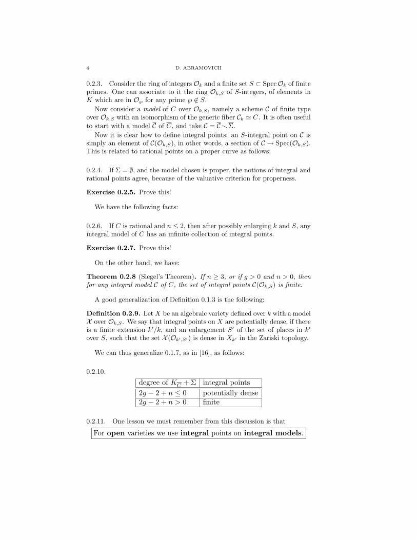

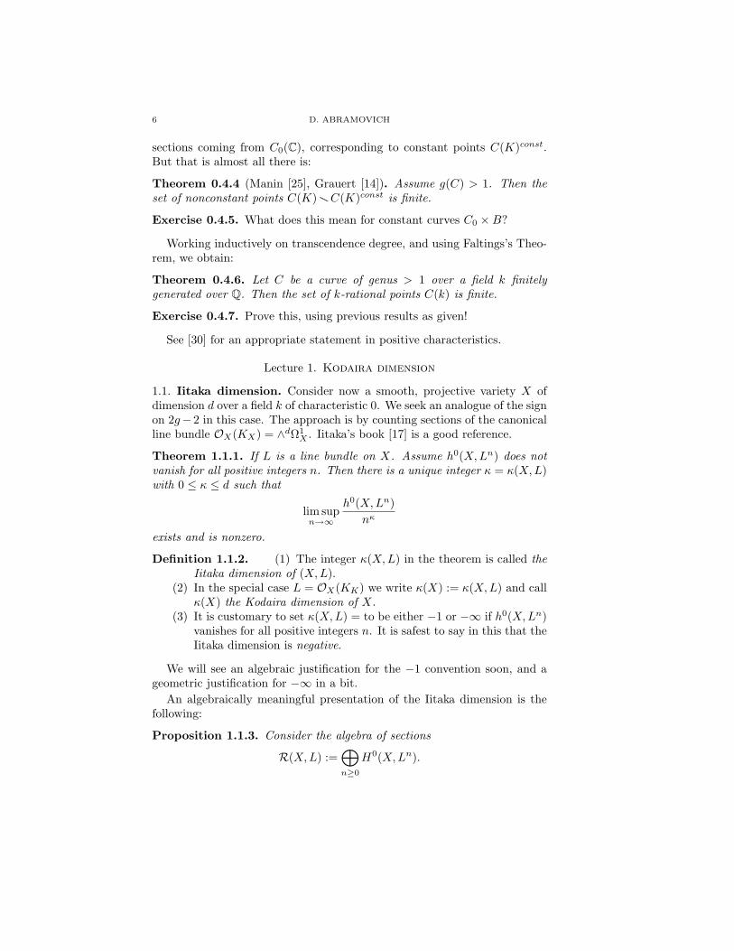


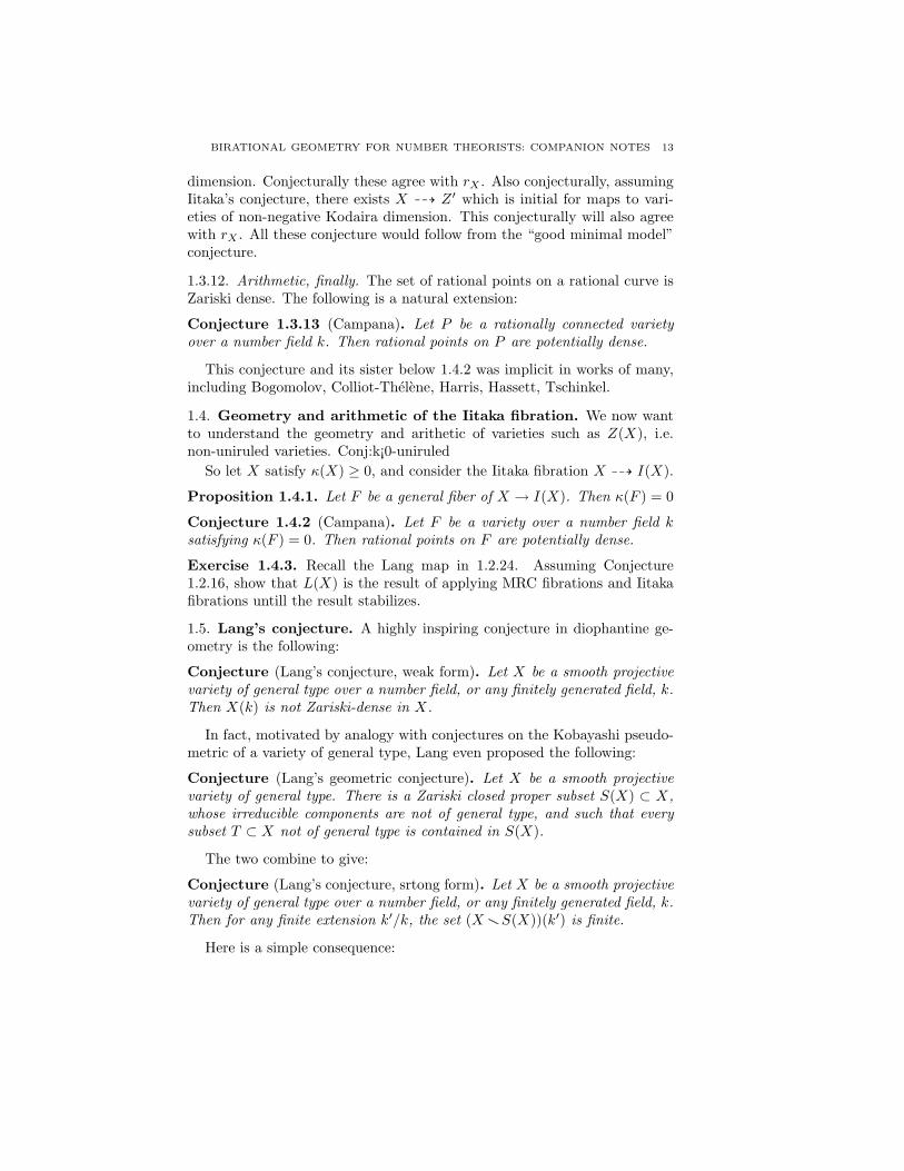
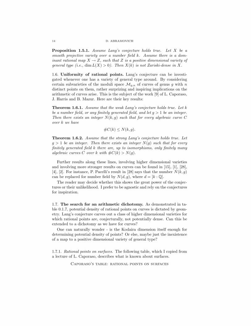
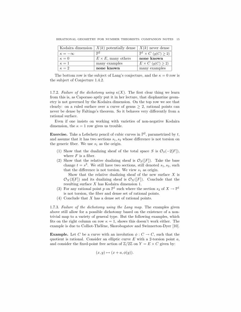

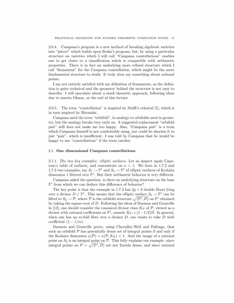


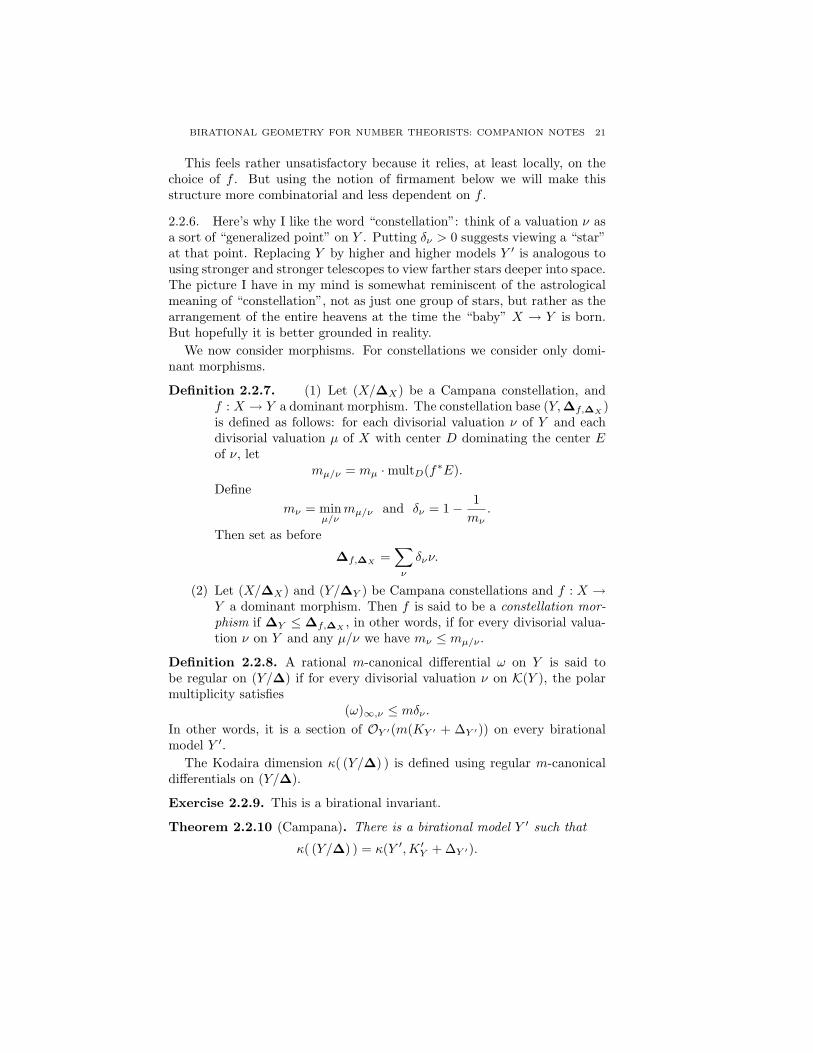


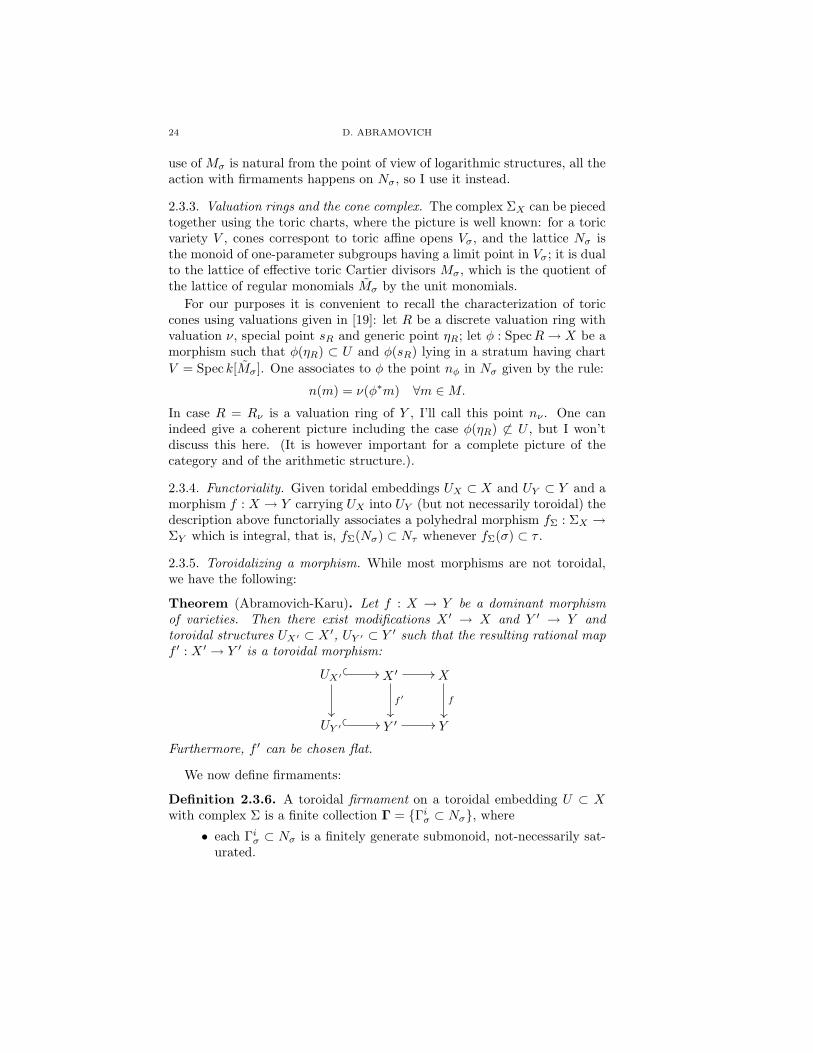

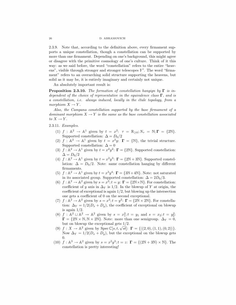


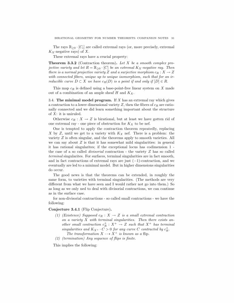


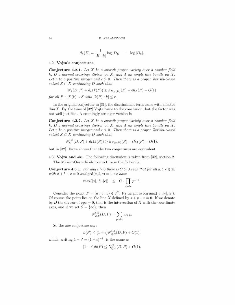


![Arithmetic Geometry for Physicists€¦ · Arithmetic Geometry for Physicists MinhyongKim Seoul,August,2017. I.Splittingprimes. Splitting primes Givenapolynomialf 2Z[x],thesetofsplittingprimes](https://static.documents.pub/doc/80x56/5fb9608667c4f77b9f79c780/arithmetic-geometry-for-physicists-arithmetic-geometry-for-physicists-minhyongkim.jpg)


