Geometry Modeling

1

EMPro 2012October 2012

Geometry Modeling

Geometry Modeling

2

© Agilent Technologies, Inc. 2000-20115301 Stevens Creek Blvd., Santa Clara, CA 95052 USANo part of this documentation may be reproduced in any form or by any means (includingelectronic storage and retrieval or translation into a foreign language) without prioragreement and written consent from Agilent Technologies, Inc. as governed by UnitedStates and international copyright laws.

AcknowledgmentsMentor Graphics is a trademark of Mentor Graphics Corporation in the U.S. and othercountries. Microsoft®, Windows®, MS Windows®, Windows NT®, and MS-DOS® are U.S.registered trademarks of Microsoft Corporation. Pentium® is a U.S. registered trademarkof Intel Corporation. PostScript® and Acrobat® are trademarks of Adobe SystemsIncorporated. UNIX® is a registered trademark of the Open Group. Java™ is a U.S.trademark of Sun Microsystems, Inc. SystemC® is a registered trademark of OpenSystemC Initiative, Inc. in the United States and other countries and is used withpermission. MATLAB® is a U.S. registered trademark of The Math Works, Inc.. HiSIM2source code, and all copyrights, trade secrets or other intellectual property rights in and tothe source code in its entirety, is owned by Hiroshima University and STARC.

The following third-party libraries are used by the NlogN Momentum solver:

"This program includes Metis 4.0, Copyright © 1998, Regents of the University ofMinnesota", http://www.cs.umn.edu/~metis , METIS was written by George Karypis(karypis@cs.umn.edu).

Intel@ Math Kernel Library, http://www.intel.com/software/products/mkl

SuperLU_MT version 2.0 - Copyright © 2003, The Regents of the University of California,through Lawrence Berkeley National Laboratory (subject to receipt of any requiredapprovals from U.S. Dept. of Energy). All rights reserved. SuperLU Disclaimer: THISSOFTWARE IS PROVIDED BY THE COPYRIGHT HOLDERS AND CONTRIBUTORS "AS IS"AND ANY EXPRESS OR IMPLIED WARRANTIES, INCLUDING, BUT NOT LIMITED TO, THEIMPLIED WARRANTIES OF MERCHANTABILITY AND FITNESS FOR A PARTICULAR PURPOSEARE DISCLAIMED. IN NO EVENT SHALL THE COPYRIGHT OWNER OR CONTRIBUTORS BELIABLE FOR ANY DIRECT, INDIRECT, INCIDENTAL, SPECIAL, EXEMPLARY, ORCONSEQUENTIAL DAMAGES (INCLUDING, BUT NOT LIMITED TO, PROCUREMENT OFSUBSTITUTE GOODS OR SERVICES; LOSS OF USE, DATA, OR PROFITS; OR BUSINESSINTERRUPTION) HOWEVER CAUSED AND ON ANY THEORY OF LIABILITY, WHETHER INCONTRACT, STRICT LIABILITY, OR TORT (INCLUDING NEGLIGENCE OR OTHERWISE)ARISING IN ANY WAY OUT OF THE USE OF THIS SOFTWARE, EVEN IF ADVISED OF THEPOSSIBILITY OF SUCH DAMAGE.

AMD Version 2.2 - AMD Notice: The AMD code was modified. Used by permission. AMDcopyright: AMD Version 2.2, Copyright © 2007 by Timothy A. Davis, Patrick R. Amestoy,and Iain S. Duff. All Rights Reserved. AMD License: Your use or distribution of AMD or anymodified version of AMD implies that you agree to this License. This library is freesoftware; you can redistribute it and/or modify it under the terms of the GNU LesserGeneral Public License as published by the Free Software Foundation; either version 2.1 ofthe License, or (at your option) any later version. This library is distributed in the hopethat it will be useful, but WITHOUT ANY WARRANTY; without even the implied warranty of

Geometry Modeling

3

MERCHANTABILITY or FITNESS FOR A PARTICULAR PURPOSE. See the GNU LesserGeneral Public License for more details. You should have received a copy of the GNULesser General Public License along with this library; if not, write to the Free SoftwareFoundation, Inc., 51 Franklin St, Fifth Floor, Boston, MA 02110-1301 USA Permission ishereby granted to use or copy this program under the terms of the GNU LGPL, providedthat the Copyright, this License, and the Availability of the original version is retained onall copies.User documentation of any code that uses this code or any modified version ofthis code must cite the Copyright, this License, the Availability note, and "Used bypermission." Permission to modify the code and to distribute modified code is granted,provided the Copyright, this License, and the Availability note are retained, and a noticethat the code was modified is included. AMD Availability:http://www.cise.ufl.edu/research/sparse/amd

UMFPACK 5.0.2 - UMFPACK Notice: The UMFPACK code was modified. Used by permission.UMFPACK Copyright: UMFPACK Copyright © 1995-2006 by Timothy A. Davis. All RightsReserved. UMFPACK License: Your use or distribution of UMFPACK or any modified versionof UMFPACK implies that you agree to this License. This library is free software; you canredistribute it and/or modify it under the terms of the GNU Lesser General Public Licenseas published by the Free Software Foundation; either version 2.1 of the License, or (atyour option) any later version. This library is distributed in the hope that it will be useful,but WITHOUT ANY WARRANTY; without even the implied warranty of MERCHANTABILITYor FITNESS FOR A PARTICULAR PURPOSE. See the GNU Lesser General Public License formore details. You should have received a copy of the GNU Lesser General Public Licensealong with this library; if not, write to the Free Software Foundation, Inc., 51 Franklin St,Fifth Floor, Boston, MA 02110-1301 USA Permission is hereby granted to use or copy thisprogram under the terms of the GNU LGPL, provided that the Copyright, this License, andthe Availability of the original version is retained on all copies. User documentation of anycode that uses this code or any modified version of this code must cite the Copyright, thisLicense, the Availability note, and "Used by permission." Permission to modify the codeand to distribute modified code is granted, provided the Copyright, this License, and theAvailability note are retained, and a notice that the code was modified is included.UMFPACK Availability: http://www.cise.ufl.edu/research/sparse/umfpack UMFPACK(including versions 2.2.1 and earlier, in FORTRAN) is available athttp://www.cise.ufl.edu/research/sparse . MA38 is available in the Harwell SubroutineLibrary. This version of UMFPACK includes a modified form of COLAMD Version 2.0,originally released on Jan. 31, 2000, also available athttp://www.cise.ufl.edu/research/sparse . COLAMD V2.0 is also incorporated as a built-infunction in MATLAB version 6.1, by The MathWorks, Inc. http://www.mathworks.com .COLAMD V1.0 appears as a column-preordering in SuperLU (SuperLU is available athttp://www.netlib.org ). UMFPACK v4.0 is a built-in routine in MATLAB 6.5. UMFPACK v4.3is a built-in routine in MATLAB 7.1.

Errata The ADS product may contain references to "HP" or "HPEESOF" such as in filenames and directory names. The business entity formerly known as "HP EEsof" is now partof Agilent Technologies and is known as "Agilent EEsof". To avoid broken functionality andto maintain backward compatibility for our customers, we did not change all the namesand labels that contain "HP" or "HPEESOF" references.

Warranty The material contained in this document is provided "as is", and is subject to

Geometry Modeling

4

being changed, without notice, in future editions. Further, to the maximum extentpermitted by applicable law, Agilent disclaims all warranties, either express or implied,with regard to this documentation and any information contained herein, including but notlimited to the implied warranties of merchantability and fitness for a particular purpose.Agilent shall not be liable for errors or for incidental or consequential damages inconnection with the furnishing, use, or performance of this document or of anyinformation contained herein. Should Agilent and the user have a separate writtenagreement with warranty terms covering the material in this document that conflict withthese terms, the warranty terms in the separate agreement shall control.

Technology Licenses The hardware and/or software described in this document arefurnished under a license and may be used or copied only in accordance with the terms ofsuch license. Portions of this product include the SystemC software licensed under OpenSource terms, which are available for download at http://systemc.org/ . This software isredistributed by Agilent. The Contributors of the SystemC software provide this software"as is" and offer no warranty of any kind, express or implied, including without limitationwarranties or conditions or title and non-infringement, and implied warranties orconditions merchantability and fitness for a particular purpose. Contributors shall not beliable for any damages of any kind including without limitation direct, indirect, special,incidental and consequential damages, such as lost profits. Any provisions that differ fromthis disclaimer are offered by Agilent only.

Restricted Rights Legend U.S. Government Restricted Rights. Software and technicaldata rights granted to the federal government include only those rights customarilyprovided to end user customers. Agilent provides this customary commercial license inSoftware and technical data pursuant to FAR 12.211 (Technical Data) and 12.212(Computer Software) and, for the Department of Defense, DFARS 252.227-7015(Technical Data - Commercial Items) and DFARS 227.7202-3 (Rights in CommercialComputer Software or Computer Software Documentation).

Geometry Modeling

5

Using the Geometry Workspace . . . . . . . . . . . . . . . . . . . . . . . . . . . . . . . . . . . . . . . . . . . . . . 6 Creating Objects in EMPro . . . . . . . . . . . . . . . . . . . . . . . . . . . . . . . . . . . . . . . . . . . . . . . . . . 15

Using the Create Extrude Window . . . . . . . . . . . . . . . . . . . . . . . . . . . . . . . . . . . . . . . . . . . 16 Creating New Objects . . . . . . . . . . . . . . . . . . . . . . . . . . . . . . . . . . . . . . . . . . . . . . . . . . . 22 Creating Bondwire Objects . . . . . . . . . . . . . . . . . . . . . . . . . . . . . . . . . . . . . . . . . . . . . . . . 24 Creating Equation-based Objects . . . . . . . . . . . . . . . . . . . . . . . . . . . . . . . . . . . . . . . . . . . . 29

Performing Operations on Objects . . . . . . . . . . . . . . . . . . . . . . . . . . . . . . . . . . . . . . . . . . . . 32 Using Locators and Cutting Planes . . . . . . . . . . . . . . . . . . . . . . . . . . . . . . . . . . . . . . . . . . . 33 Modifying Existing 2D and 3D Objects . . . . . . . . . . . . . . . . . . . . . . . . . . . . . . . . . . . . . . . . 39 Performing Boolean Operations . . . . . . . . . . . . . . . . . . . . . . . . . . . . . . . . . . . . . . . . . . . . . 44 Using Geometry Modeling Tools . . . . . . . . . . . . . . . . . . . . . . . . . . . . . . . . . . . . . . . . . . . . 50

Orienting Objects in the Simulation Space . . . . . . . . . . . . . . . . . . . . . . . . . . . . . . . . . . . . . . . 76 Materials . . . . . . . . . . . . . . . . . . . . . . . . . . . . . . . . . . . . . . . . . . . . . . . . . . . . . . . . . . . . . . 88

Materials Overview . . . . . . . . . . . . . . . . . . . . . . . . . . . . . . . . . . . . . . . . . . . . . . . . . . . . . 89 Selecting a Material . . . . . . . . . . . . . . . . . . . . . . . . . . . . . . . . . . . . . . . . . . . . . . . . . . . . . 91 Assigning Materials to Objects . . . . . . . . . . . . . . . . . . . . . . . . . . . . . . . . . . . . . . . . . . . . . 110

Geometry Modeling

6

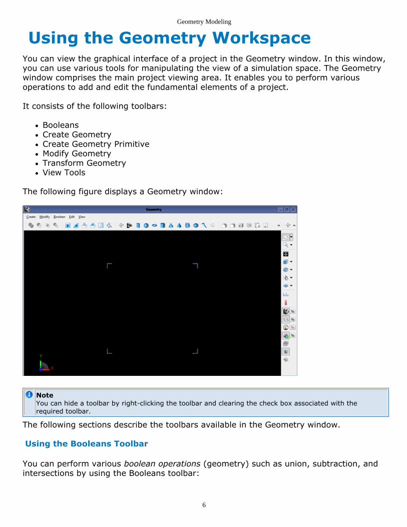
Using the Geometry WorkspaceYou can view the graphical interface of a project in the Geometry window. In this window,you can use various tools for manipulating the view of a simulation space. The Geometrywindow comprises the main project viewing area. It enables you to perform variousoperations to add and edit the fundamental elements of a project.

It consists of the following toolbars:

BooleansCreate GeometryCreate Geometry PrimitiveModify GeometryTransform GeometryView Tools

The following figure displays a Geometry window:

NoteYou can hide a toolbar by right-clicking the toolbar and clearing the check box associated with therequired toolbar.

The following sections describe the toolbars available in the Geometry window.

Using the Booleans Toolbar

You can perform various boolean operations (geometry) such as union, subtraction, andintersections by using the Booleans toolbar:

Geometry Modeling

7

The following table describes options available on the Booleans toolbar:

Option Icon Description

Union Enables you to unite two objects in the Geometry workspace.

Subtract Enables you to subtract objects in the Geometry workspace.

Intersect Enables you to intersect two objects in the Geometry workspace.

Chop Enables you to cut objects in the Geometry workspace.

Using the Create Geometry Toolbar

The Create Geometry toolbar provides options for creating new objects.

The following table describes options available on the Create Geometry toolbar:

Option Icon Description

Extrude Enables you to extrude objects in the Geometry workspace.

Revolve Enables you to revolve objects in the Geometry workspace.

Extrude from Face Enables you to extrude objects from face in the Geometry workspace.

Revolve from Face Enables you to rotate objects from face in the Geometry workspace.

Sheet Body fromFaces

Enables you to create sheet body objects from faces in the Geometryworkspace.

Wire Body Enables you to create wire body objects in the Geometry workspace.

Using the Create Geometry Primitive

The Create Geometry Primitive toolbar provides options for creating parameterized 3Dobjects that includes various types of shapes such as Bondwire, Box, Sphere, Torus,Prism, Pyramid, Frustum, and Helix.

The following table describes options available on the Create Geometry Primitive toolbar:

Geometry Modeling

8

Option Icon Description

Assembly Enables you to add an Assembly object in Parts.

Box Enables you to create a box structure in the Geometry workspace. You can specify theorientation, width, height, and width of the box.

Sphere Enables you to create a sphere in the Geometry workspace. You can specify the orientationand edit properties of the sphere.

Torus Enables you to create a Torus object in the Geometry workspace. You can specify theorientation, major radius, and minor radius values for the Torus object.

Prism Enables you to create a Prism object in the Geometry workspace. You can specify theorientation, height, base radius, and number of sides for the Prism object.

Pyramid Enables you to create a Pyramid object in the Geometry workspace. You can specify theorientation, height, base radius, top radius, and number of sides for the Pyramid object.

Frustum Enables you to create a Frustum object in the Geometry workspace. You can specify theorientation, height, base radius and top radius for the Frustum object.

Helix Enables you to create a Helix object in the Geometry workspace. You can specify theorientation, height, radius, wire diameter, number of threads, profile and path segments,and handedness for the Helix object.

Solderball Enables you to create a Solderball object in the Geometry workspace. You can specify theorientation, height, end face width, solder ball width, divisions, and arc resolution for theSolderball object.

Bondwire Enables you to create a Bondwire object in the Geometry workspace. You can specify theorientation, fixed positions, and definition for the Bondwire object.

EquationBased

Enables you to specify an equation in the Geometry workspace. You can specify theorientation and edit an equation.

Using the Modify Geometry Toolbar

The Modify Geometry toolbar provides options for modifying the geometry of objects.

The following table describes options available on the Modify Geometry toolbar:

Option Icon Description

Chamfer Edges Enables you to chamfer the selected edges of an object.

Blend Edges Enables you to blend the selected edges of an object.

Shell Enables you to select the faces to remain opened for an object.

Remove Faces Enables you to remove selected faces of an object.

Offset Faces Enables you to offset selected faces of an object.

Offset SheetEdges

Enables you to select the edges to offset and specify the edge offsetvalue.

Thicken Sheet Enables you to specify the distance and option for thickening both sides.

Loft Faces Enables you to select faces to loft on an object.

Using the Transform Geometry Toolbar

Geometry Modeling

9

The Transform Geometry toolbar provides options for transforming the geometry ofobjects.

The following table describes options available on the Transform Geometry toolbar:

Option Icon Description

SpecifyOrientation

Enables you to specify the orientation of an object.

Scales Enables you to scale an object by specifying the U, V, and W values.

Translate Enables you to specify the translation values for an object.

Rotate Enables you to rotate an object by specifying the angle to rotate, axis point, and axisdirection. You can also preview your required settings.

Reflect Enables you to specify the plane point and normal values. You can also preview yourrequired settings.

Shear Enables you to specify the shear values.

Using the View Tools Toolbar

You can use the View Tools toolbar to modify the perspective of viewing the Geometrywindow by manual rotation, translation, and zoom, as well as automatic orientations toachieve the required perspective. You can access View Tools from the right-hand side ofthe Geometry window or select View. The following figure displays the View Toolsoptions:

Geometry Modeling

10

Using View Manipulation Options

The View Manipulation menu provides the following options:

Select: The Select tool is the default tool in the Geometry workspace window. It isused to select objects as well as manipulate the view of the simulation space.

Rotation about a fixed point:Left-click and drag.Click the mouse wheel and drag.

Translation (panning):Right-click and drag.Hold Shift, left- or right-click and drag.

Zooming:Roll the mouse wheel backwards or forwards (to zoom-in or zoom-out,respectively).Hold Ctrl, left-click and drag the mouse up or down (to zoom-in or zoom-out,respectively).

Orbit: The Orbit tool is selected to perform rotation of the simulation space throughleft-clicking-and-dragging.

Pan: The Pan Tool tool is selected to perform translation of the simulation space

Geometry Modeling

11

through left-clicking-and-dragging.

Zoom: Zoom-in or zoom-out of simulation space by left-clicking-and-dragging themouse up or down, respectively.

Zoom to Window: Zoom into a rectangular shaped area of the geometry as specifiedby the user. To use, select the tool, then left-click and drag the mouse to designatethe rectangular zoom area.

Zoom to Extents: Select this tool to automatically zoom so that the entire geometrycan be viewed in the simulation space.

Standard View, Isometric View, and Custom View

The Standard Views and Isometric Views buttons function to automatically change theperspective of the objects in the Geometry workspace window.

Isometric Views

The Standard View changes the view to the following orientations:

Front (-Y)Back (+Y)Top (-Z)Bottom (+Z)Right (-X)Left (+X)

The Isometric View changes the perspective to any combination of these views:

Front/Right/TopFront/Left/TopFront/Right/BottomFront/Left/BottomBack/Right/TopBack/Left/TopBack/Right/BottomBack/Left/Bottom

If these buttons do not achieve the desired perspective, use the Select, Orbit or Pan toolsto customize the orientation, and save the desired view by clicking the Custom Views >Add View button.

Cutting Planes

Using the cutting plane options, you can reorient a cutting plane, save orientation of thecurrent cutting plane, and open previously saved orientations.When the cutting plane feature is active, it clips the entire geometry in the positive Zdirection. You can use this feature to toggle a cutting plane.

Geometry Modeling

12

To enable the cutting plane feature, select View > Cutting Planes > Toggle CuttingPlane in the Geometry workspace. To deactivate, again select View > Cutting Planes >Toggle Cutting Plane. You can also select this option by clicking the Cutting plane iconon the toolbar, as shown in the following figure:

For more information about how to use the cutting plane feature, see Snap Objects UsingCutting Plane (geometry).

Measure Tool

This tool measures the 3-D distance between any two points by left-clicking on a startingpoint and dragging to an ending point. A box in the lower-right corner of the GUI displaysthe coordinates of the cursor position in 3-D space. A box in the lower-left corner of theGUI displays axis-aligned distances. The following illustration shows the Measure Toolcalculating the distance between the corners of a rectangle.

Field Reader Tool

Geometry Modeling

13

The Field Reader tool measures field values at the location where the mouse hovers overthe geometry. For more information on the field reader tool, see Viewing FDTD DefaultOutput (fdtd).

Export Image Tool

The Export Image tool takes a screen shot of the geometry as it is currently shown in theGeometry workspace window, and saves it to a specified location.

Opacity and Visibility Tools

The Visibility buttons control the view of parts of the project.

Clicking any of these buttons will hide its corresponding objects. They include:

Parts View - Toggles the geometric parts on and off.Circuit Components View - Toggles the circuit components on and off.Sensors View - Toggles the sensors on and off.Result Fields View - Toggles the result fields on and off.

Clicking the Opacity button located to the right of any button, will bring up a slider tocustomize the translucency of its objects. The sliders change the alpha of the objects,making them more or less translucent as the slider is dragged right or left, respectively.When the project is in Mesh View mode, these buttons are convenient for turning off theview of the solid geometry so that the view of the cell edges is not obstructed.

Geometry Modeling

14

NoteThere are several ways EMPro can render this translucency. For more information on how to adjust thesesettings the notes on Transparency Algorithm, see Specifying Global Options (global).

Toggle Bounding Box Visibility

This button toggles the visibility of the bounding box for the geometry when the geometryis selected.

Toggle Output Viewing Controls

This button toggles the visibility of the output viewing controls for sensor results.

Geometry Modeling

15

Creating Objects in EMProEMPro provides feature-based modeling that allows the creation of geometric objects as aset of repeatable actions rather than one stringent primitive object. This provides moreflexibility in customizing an object and reverts any step without using excess memory thatwas formally required to rebuild an entire object. It also tracks every step in the modelingsequence as a separate object in the tree to facilitate even simpler additions, deletionsand modifications to the modeling sequence. You can create new objects, create objectsfrom the existing objects, and 3D components in the Geometry workspace.

This section provides information about the following topics:

Using the Create Extrude Window (geometry)Creating New Objects (geometry)Creating Bondwire Objects (geometry)Creating Equation-based Objects (geometry)

Geometry Modeling

16

Using the Create Extrude WindowYou can create new objects or modify existing objects to create new objects by using theCreate Geometry toolbar. To create 3D components, use the options available on theCreate Geometry Primitive toolbar.

To create new objects, click Extrude on the Create Geometry toolbar to display theCreate Extrude window. The following figure displays options present in the CreateExtrude window:

This window consists of three tabs: Specify Orientation, Edit Cross Section, and Extrude.You can specify the required orientation for an object in the Specify Orientation(geometry) tab. In the Extrude tab, specify the extrude distance. You can set objectproperties in the Edit Cross Section tab. This section describes the options present in theEdit Cross Section tab.

Edit Cross Section Tab Overview

The Edit Cross Section tab consists of Shapes, Constraints, Tools, Snapping optionbuttons. By default, all the four set of option buttons are selected. However, you can clearthe check box associated with each option to remove the corresponding set of toolbars.You can also access these options the drop-down menus in the upper-left part of thescreen.

Using the following option buttons, you can create various types of objects in theGeometry workspace:

Shapes

The Edit Cross Section tab contains a number of Shapes sketching tools that are useful forcreating simple 2D geometries for wire bodies and sheet bodies. They also serve as acommon starting point to define 2D cross sections for 3D bodies such as extrusions,revolutions, and more complicated solid modeling operations. The Shapes tools areselected by clicking their respective icon.

Pressing Esc or Backspace will back-up one step when using a multistep creation

Geometry Modeling

17

tool.Pressing Esc a second time will deactivate the edge creation tool and activate thedefault Select tool.Pressing Tab will bring up a dialog to specify the position.

The following types of 2D shapes are available in EMPro:

Straight EdgePolyline EdgePerpendicular EdgeTangent LineRectanglePolygonN-Sided Polygon3-Point ArcArc Center, 2 Points2-Point ArcCircle Center, Radius3-Point Circle2-Point CircleEllipse

NoteFor a detailed description of each shape tool, refer to Shapes (geometry).

Tools: The Tools buttons provide useful functionality to users while sketching in the 2-Dsketcher.

Select/ManipulateTrim CurvesInsert VertexFillet Vertex

NoteFor a detailed description of each 2-D sketcher tool, refer to Tools (geometry).

Constraints

Constraints are restrictions placed on geometric parts that must be satisfied in order toconsider the model valid. They ensure that the user's intent is sustained throughout acalculation when parameters may change. Some objects are created with constraintsalready embedded. For instance, a rectangle is composed of four straight edges that areconstrained perpendicularly as seen in preceding illustration. Other constraints are user-defined by using the Constraint tools.

Applying a constraint to an object will often affect other characteristics of the object. Forinstance, applying a horizontal constraint to one side of an irregular quadrilateral will mostlikely change the length of one or more sides and the angles that form with thoseconnecting sides. Thus, it is important to lock any points that are intended to stay static.There are two main ways to do this:

Geometry Modeling

18

By selecting the Lock Constraint tool and clicking the the appropriate vertex or side.By selecting the Select/Manipulate tool, right-clicking the appropriate vertex or side,and selecting Lock Position, as shown below.

The following figure displays the locking or editing a vertex's position with theSelect/Manipulate tool:

NoteFor more about the Select/Manipulate tool's functionality, refer to Select/Manipulate (geometry).

Each type of the following types of Constraint tools has its own green symbol or letter thatis visible when the mouse is held over the constrained segment.

HorizontalVerticalCollinearParallelPerpendicularTangentConcentricAngleDistanceEqual LengthEqual DistanceRadiusEqual Radius

NoteFor a detailed description of each constraint, refer to Constraints (geometry).

Snapping

Snapping tools are available to facilitate the exact placement of vertices on the sketchingplane. When snapping is enabled, the mouse will be snapped to the closest of one or

Geometry Modeling

19

more snapping landmarks if one comes within range. For example, if Snap To Grid Lines isselected, the mouse is moved or snapped to points on the closest grid line as it is movedaround in the sketching plane. This makes it much easier to place a vertex in the desiredposition without having to zoom in to a discrete position. Blue dots and blue linesrepresent the snapped location of the mouse when snapping is enabled.

In the case that the mouse is not within sufficient range of a selected landmark listedbelow, a vertex will be placed at its exact location on the sketching plane as if snappingwere not turned on. (For example, if the mouse is dragged to the middle of a cell and theSnap To Grid Lines option is selected, the vertex will be placed in the center of the cellbecause it is not close enough to a surrounding grid line.)

NoteFor snapping objects using the cutting plane feature, see Snapping Objects with Cutting Planes(geometry).

Several snapping options can be selected at a time, in which case, the vertex will besnapped to the closest landmark that is within range of the mouse.

Snap To Grid LinesSnap To Grid/Edge IntersectionsSnap To VerticesSnap To EdgesSnap To Edge/Edge Intersections

NoteFor a detailed description and image of each, refer to Snapping (geometry).

Customizing the Construction Grid

The Construction Grid controls the appearance of the grid without impacting its actual cellsize. In addition to these options, the Edit Cross Section tab consists of the ConstructionGrid button. Click Construction Grid to edit the spacing of the visible grid lines in the 2-D sketcher. (This has no impact on the FDTD grid definition). The following figure displaysa Construction grid:

It provides the following options:

Automatically Adjust Line Spacing causes the construction grid to adjust its line

Geometry Modeling

20

spacing with the current zoom level. As you zoom in, the lines are moved to be closerto each other. As you zoom out, they decimate and become further apart.Line Spacing is available when automatic isn't checked. This is the spacing betweenadjacent lines of the construction grid.Highlight Interval controls the interval which lines are highlighted. Every "Nth" linewill be made bold.Mouse Spacing controls the minimum resolvable distance by the mouse. As you movethe mouse, you will be unable to move between two points closer than this specifieddistance.

3D Operation Tabs

If subsequent tabs are available to the right of the Edit Cross Section tab, continue on tocomplete a 3-D operation. (These tabs are not available for 2-D objects.)

The figure below shows the Advanced drop-down menu inside of the Extrude tab,available when an Extrude operation is selected. This menu contains operations that canbe applied to the 3D object. For more information on these operations, see Advanced 3-DSolid Modeling Operations (geometry).

Using the Create Geometry Primitive Toolbar

The Create Geometry Primitive Toolbar consists of a library of parameterized 3D objects

Geometry Modeling

21

that includes various types of shapes: Bondwire, Box, Sphere, Torus, Prism, Pyramid,Frustum, Helix, Solder Ball, and Equation Based.

Geometry Modeling

22

Creating New ObjectsYou can create new objects in the Geometry workspace by using the Extrude, Revolve,and Wire Body options available on the Create Geometry toolbar.

To create a new object by using the extrude option:

Click Extrude ( ) on the Create Geometry toolbar.1.Type a name for the object in the Name text box.2.Click the Specify Orientation tab. The orientation options are displayed, as shown3.in the following figure:

Set the orientation of the drawing plane. The default orientation is XY plane. For4.more information, see Orienting Objects in the Simulation Space (geometry).Click the Edit Cross Section tab. For more information, see Edit Cross Section Tab5.Overview (geometry).Draw 2D objects such as circle, rectangle, or polygons. The following figure displays a6.rectangle:

Click the Extrude tab.7.Specify the extrude options, as shown in the following figure:8.

Geometry Modeling

23

NoteYou can modify the existing objects by using the Extrude From Face, Revolve From Face, Sheet BodyFrom Face options to create new objects.

You can also use the Create Geometry Primitive toolbar for creating new objects. Itconsists of a library of parameterized 3D objects that includes various types of shapes:Bondwire, Box, Sphere, Torus, Prism, Pyramid, Frustum, Helix, Solder Ball, and EquationBased. A shape can be inserted by selecting the appropriate item from the Create Newmenu. With each of these shapes corresponds an editing tool, that lets you specify theshape parameters. By double clicking the building block in the Part node of the ProjectTree, one can (re)edit the parameters after insertion.

Geometry Modeling

24

Creating Bondwire ObjectsBondwire objects allow you to create interconnections between an integrated circuit (IC)and a printed circuit board (PCB) during semiconductor device fabrication. It can also beused to connect an IC to other electronics or to connect from one PCB to another.

To create a Bondwire object:

Click Extrude ( ) on the Create Geometry toolbar.1.

Select the Rectangle tool in the Geometry-Create Extrude window and draw a2.rectangular shaped object. The following figure displays the rectangle object:

Click the Extrude tab and modify the parameters.3.Click Done. The rectangular shape is visible in the Geometry window.4.

Similarly, create a circular shape in the Geometry window. The following figure displaysthe final geometry:

Creating Bondwire

Geometry Modeling

25

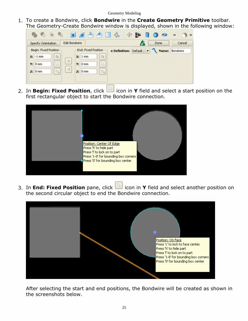
To create a Bondwire, click Bondwire in the Create Geometry Primitive toolbar.1.The Geometry-Create Bondwire window is displayed, shown in the following window:

In Begin: Fixed Position, click icon in Y field and select a start position on the2.first rectangular object to start the Bondwire connection.

In End: Fixed Position pane, click icon in Y field and select another position on3.the second circular object to end the Bondwire connection.

After selecting the start and end positions, the Bondwire will be created as shown inthe screenshots below.

Geometry Modeling

26

Click Done to complete the Bondwire creation. The Bondwire is displayed in the4.Geometry window.

Editing Bondwire Definition

To edit the Bondwire definition:

In the Definitions branch of the project tree, choose Bondwire Definition >1.

Geometry Modeling

27

Default JEDEC. JEDEC is a standard for Bondwire profiles. In EMPro, the Bondwiredefinitions are more general and do not have to implement JEDEC profiles. Thedefault Bondwire definition is a JEDEC profile as an example.Edit the Bondwire definitions in the Bondwire Definition Editor window.2.

The Bondwire Definition Editor consists of three parts: Crossection, profile and preview.

Crossection:

Bondwires have a polygonal cross section. You can choose the radius and the number ofsides.

Preview:

Here you can view a preview of the profile. There are two parameters to steer this, thepreview length which is the horizontal distance between beginning and the end point. Theheight difference which is the vertical distance between begin and end point. These values

Geometry Modeling

28

are not properties of the Bondwire definition. These are just two values necessary for apreview.

Profile:

Each profile consists of a number of vertices between a beginning and endpoint. Thebeginning and endpoints will be choosen when a Bondwire is created so they are not partof the definition.

The vertices are defined by horizontal and vertical offsets in the vertical plane passingthrough beginning and endpoint. Each offset value is accompanied by a type and areference:

Reference: Offsets are added to the horizontal or vertical position of the Previousvertex, Begin or End point (horizontal offsets are subtracted from the End pointinstead). When selecting a vertex in the editor, green markers will highlight thechosen references.Type: Each offset is either an absolute Length, Proportional to the horizontal distancebetween begin- and end point, or specifies an Angular constraint.Length: The offset is an absolute length, and will be identical for all bondwires thatuse this definition.Proportional: The offset is proportional to the horizontal distance between begin- andend point, and the exact offset can differ between different bondwires. Use this fordefinitions that need to stretch depending on the location of the bondwire.Angular: For each vertex, at most one of the offsets can be of the Angular type. Itwill put a constraint on the angle between the horizontal line and the line passingthrough the vertex and reference point. If both offsets of a single vertex are Angular,the vertex is invalid.

Geometry Modeling

29

Creating Equation-based ObjectsUsing the Equation Based option, you can create objects with predefined settings. You canuse the existing settings for creating various objects such as Ellipsoid, Hyperbolic,Hyperboloid, Paraboloid, XY-plane, XZ-plane, and YZ-plane. The Create Equation windowconsists of predefined objects in the Presets section, as shown in the following figure:

To create an equation-based object:

Open the Geometry window.1.Select Create > Geometry > Equation Based in the Geometry window. The Create2.Equation window is displayed.In the Edit Equation tab, select an option from Presets. For example, in the3.following figure, Ellipsoid is selected:

Click . The default values associated with the preset object are populated in4.Dimensions fields.Click the Specify Orientation tab.5.Verify the orientation settings.6.Type an equation name.7.Click Done. You have created a new object. For example, the following figure8.displays an Ellipsoid object with the default settings:

Example- Creating a Waveguide using the Equation-based Feature

The following example shows how to do the taper waveguide using equation-basedgeometry creation tool. In this example, a waveguide is created with length 15mm in Zdirection. The cross section of the waveguide in XY plane is rectangular everywhere, withthe cross sectional dimensions X and Y a function of the length Z (z- variable), as shownin the equations below:

X(Z)= 2*\[cos(Z/15)]^2;

Geometry Modeling

30

Y(Z)= 2*\[cos(Z/15)]^2; Z varying from 0 to 15 mm

First, with the equation based feature, you will create solid bodies. If you need a solidbody, use the sheet body that is created with the equation based feature with someadditional extrude-from-faces and Boolean operations.

To create the sheet body with the specified dimensions, you need to create fourequations, i.e., one for each face.The original equations were:

x(z) = 2 * cos(z / 15)^2

y(z) = 2 * cos(z / 15)^2

z = (0 .. 15)

Thus, the parametric equations (in terms of u and v) for the edges of the Waveguide are:With u = (0 .. 15)

Edge 1

Create the following equation:

x = (2 / 2) * cos( u / 15)^2

y = (2/ 2) * cos( u / 15)^2

z = u

Edge 2

Create the following equation:

x = -(2 / 2) * cos(u / 15)^2

y = (2/ 2) * cos(u / 15)^2

z = u

Edge 3

Create the following equation:

x = -(2/ 2) * cos(u / 15)^2

y = -(2/ 2) * cos( u / 15)^2

z = u

Edge 4

Create the following equation:

x = (2/ 2) * cos(u / 15)^2

y = -(2 / 2) * cos( u / 15)^2

z = u

Geometry Modeling

31

You can easily extend the latter to face equations by using the other parameter vWith u = (0 .. 15), and v = (-1 .. 1)

Face 1

Create the following equation:

x = v *( 2/ 2) * cos( u / 15)^2

y = (2/ 2) * cos( u / 15)^2

z = u

Face 2

Create the following equation:

x = -(2/ 2) * cos( u / 15)^2

y = v * (2 / 2) * cos( u / 15)^2

z = u

Face 3

Create the following equation:

x = v * -(2 / 2) * cos( u / 15)^2

y = -(2 / 2) * cos( u / 15)^2

z = u

Face 4

Create the following equation:

x = (2 / 2) * cos( u / 15)^2

y = v * -(2 / 2) * cos( u / 15)^2

z = u

Geometry Modeling

32

Performing Operations on ObjectsYou can modify the existing objects by performing various operations such as boolean,blending edges, and changing the orientation of objects in the Geometry window. You canrearrange objects using locators and snap the vertices of objects using cutting planes.

Modifying Existing 2D and 3D Objects (geometry)Performing Boolean Operations (geometry)Using Locators and Cutting Planes (geometry)

Geometry Modeling

33

Using Locators and Cutting PlanesYou can easily move objects and place them at the required location by using locators. Inaddition, you can snap the required vertices of an object by using the cutting planefeature.

Using Locators

A locator is a triad that can be placed on a part or assembly to aid in its orientation. Itenables you to align two parts and place one part on top of one another part.

Creating a Locator

To create a locator:

Right-click an object in the Parts list and select Create New > Locator.1.

Double-click a locator to open the Edit Locator window, which is used to modify the2.location and orientation of the Locator object. The following figure displays the EditLocator window:

Specify the Global coordinates in the X, Y, and Z text boxes.3.Select Reference from the Context drop-down list.4.Specify the Reference coordinates in the U, V, and W text boxes.5.Select a value from the Presets drop-down list.6.You can also rotate, translate, specify a new direction, define two reference points, or7.point at a specified direction by using the U, V, and W drop-down list. These optionsare displayed in the following figure:

Click Advanced mode to specify translation and rotation values. You can also specify8.

Geometry Modeling

34

anchor, twist, and axis values.Click Done.9.

Reorienting Parts Using Locators

You can reorient parts by matching their locators. To do this:

Select two locators in the Project tree.1.

Right-click the selected locators and select Match Locators. The Match Locators2.dialog box is displayed, as shown in the following figure:

The Move text box defines the part that is being moved and the To Match text box3.specifies the part that remains fixed.

You can click Swap Order to reverse the default selection.

Click OK.4.

The part that will be moved by default is determined by the selection order.

How do I Rearrange Objects Using Locators

You can rearrange two objects Box1 and Box2 by using locators in the following manner:

Create a Locator

Right-click Box1 and select Create New > Locator. A new locator is added to Box1.1.Double-click the Box1 locator. The Edit Locator window is displayed.2.Select the Simple Plane tool.3.Place the locator at the center of the face of Box1.4.Click Done.5.Right-click Box2 and select Create New > Locator. A new locator is added to Box2.6.Double-click Box2 locator. The Edit Locator window is displayed.7.Select the Simple Plane tool.8.Place the locator at the center of the face of Box2.9.Click Done.10.

Rearrange Objects

Select the two locators in the project tree.1.Right-click the selected locators and select Match Locators. The Match Locators2.dialog box is displayed.

Geometry Modeling

35

Click Swap Order to reverse the default selection.3.Click OK. Box2 is placed on the top of Box1.4.

Show me How to Rearrange Objects Using Locators

Video: Rearrange Objects Using Locators

Using Cutting Planes

Using the cutting plane options, you can reorient a cutting plane, save orientation of thecurrent cutting plane, and open previously saved orientations.When the cutting plane feature is active, it clips the entire geometry in the positive Zdirection. You can use this feature to toggle a cutting plane.

Activating and Saving a Cutting Plane

To enable the cutting plane feature, select View > Cutting Planes > Toggle CuttingPlane in the Geometry workspace. To disable the feature, again select View > CuttingPlanes > Toggle Cutting Plane. You can also select this option by clicking the Cuttingplane icon on the toolbar, as shown in the following figure:

To save a cutting plane:

Select View > Cutting Planes > Save Cutting Plane. The Name Cutting Plane1.dialog box is displayed, as shown in the following figure:

Type a name for the cutting plane in the Name text box.2.Click OK.3.

Editing a Cutting Plane

To reorient a cutting plane:

Geometry Modeling

36

Select View > Cutting Planes > Edit Cutting Plane in the Geometry workspace.1.The Edit Cutting Plane window is displayed, as shown in the following figure:

Specify the Global coordinates in the X, Y, and Z text boxes.2.Select Reference from the Context drop-down list.3.Specify the Reference coordinates in the U, V, and W text boxes.4.Select a value from the Presets drop-down list.5.You can also rotate, translate, specify a new direction, define two reference points, or6.point at a specified direction by using the U, V, and W drop-down list. These optionsare displayed in the following figure:

Click Done. The following illustration shows the cutting plane tool reorienting a7.cutting plane:

Geometry Modeling

37

Snapping Objects with Cutting Planes

You can snap the vertices of two objects by using the cutting plane feature. The solidbody, sheet body, and wire body geometry that is clipped using the cutting plane toolform edges and vertices that can be used for snapping. The sketcher provides a snappingtool to toggle this behavior. The Point, direction, and plane picking tools also snap to theselocations.

Perform the following steps:

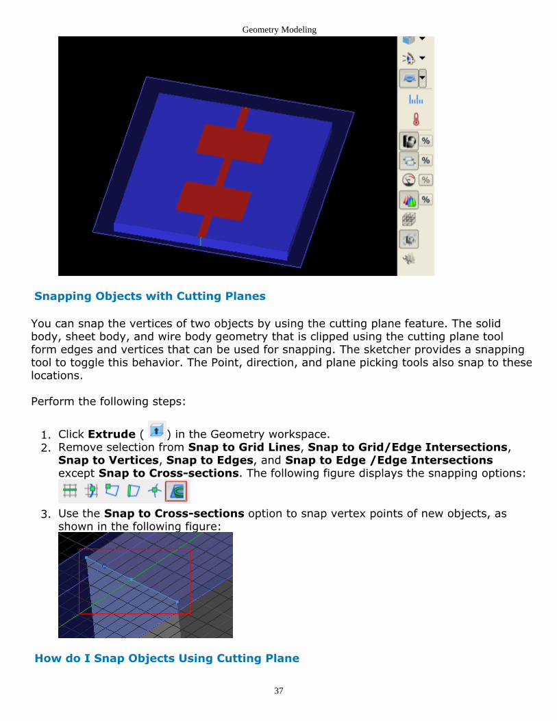
Click Extrude ( ) in the Geometry workspace.1.Remove selection from Snap to Grid Lines, Snap to Grid/Edge Intersections,2.Snap to Vertices, Snap to Edges, and Snap to Edge /Edge Intersectionsexcept Snap to Cross-sections. The following figure displays the snapping options:

Use the Snap to Cross-sections option to snap vertex points of new objects, as3.shown in the following figure:

How do I Snap Objects Using Cutting Plane

Geometry Modeling

38

You can snap objects using the cutting plane tool in the following manner:

Edit the Cutting Plane

Select Edit Cutting Plane in View tools.1.Select the Simple Plane tool.2.Position the pointer on the face of the prism.3.Click Done.4.

Snap Objects using Cutting Planes

Click Extrude in the Geometry workspace.1.Select Polyline Edge from the Shapes toolbar.2.Select the vertex points of the prism.3.Click Extrude.4.Click Done to snap vertex points of the prism object.5.Disable the Toggle Cutting Plane option to view the snapped object.6.

Show me How to Snap Objects Using Cutting Plane

Video: Snap Objects Using the Cutting Plane Feature

Geometry Modeling

39

Modifying Existing 2D and 3D ObjectsThe modeling operations applied to the object are stored in EMPro. This enables you tochange the operations according to your requirements. You can modify existinggeometries which include imported objects, for example, move, copy, rotate, and Booleanoperations. This section describes how to modify 2D and 3D objects.

Creating 3D Objects from 2D Objects

Perform the following steps for creating 3D objects from 2D objects:

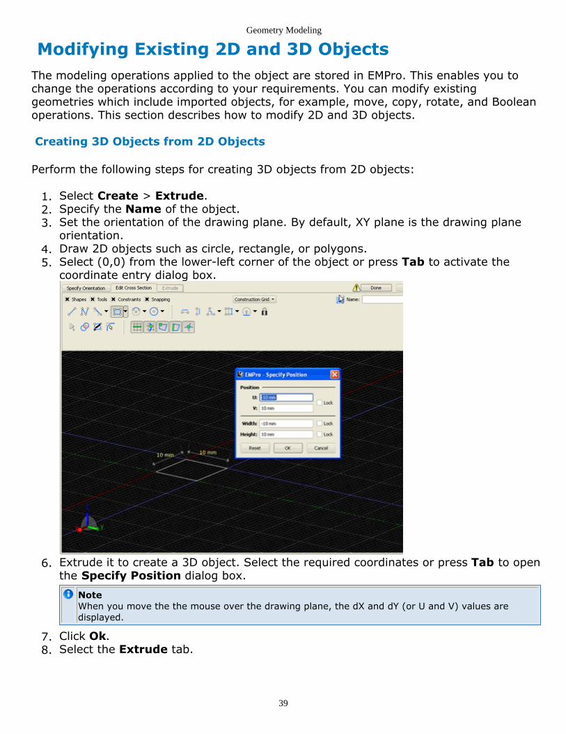
Select Create > Extrude.1.Specify the Name of the object.2.Set the orientation of the drawing plane. By default, XY plane is the drawing plane3.orientation.Draw 2D objects such as circle, rectangle, or polygons.4.Select (0,0) from the lower-left corner of the object or press Tab to activate the5.coordinate entry dialog box.

Extrude it to create a 3D object. Select the required coordinates or press Tab to open6.the Specify Position dialog box.

NoteWhen you move the the mouse over the drawing plane, the dX and dY (or U and V) values aredisplayed.

Click Ok.7.Select the Extrude tab.8.

Geometry Modeling

40

Enter a value in the in the Extrude Distance text box. You can also move the arrow9.in the geometry space to change the distance.Click Done. The green check mark means that there is no problem with this object10.creation.

Resizing Existing 3D Objects

Perform the following steps for resizing the height of an object:

Open a EMPro project.1.Expand the Parts menu and double-click Extrude.2.Open the Extrude tab and change the Extrude Distance.3.

Click Done.4.

Editing Existing Extruded 2D Object

Click Extrude to open the 2D drawing space.1.

Geometry Modeling

41

Click Select/Manipulate from Tools menu . Place the mouse over the edges or2.corners of rectangle, and right-click to open the Edit/Delete menu:

Delete the edges or select the vertices to edit or lock the positions.3.

Moving (Translating)/Rotating Objects

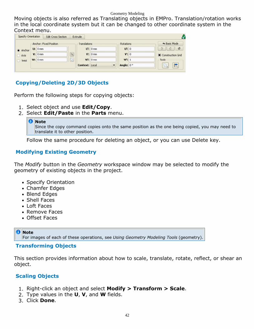
Use "Specify Orientation" menu or tab from either the Geometry modeling menu or objectcreated

Geometry Modeling

42

Moving objects is also referred as Translating objects in EMPro. Translation/rotation worksin the local coordinate system but it can be changed to other coordinate system in theContext menu.

Copying/Deleting 2D/3D Objects

Perform the following steps for copying objects:

Select object and use Edit/Copy.1.Select Edit/Paste in the Parts menu.2.

NoteSince the copy command copies onto the same position as the one being copied, you may need totranslate it to other position.

Follow the same procedure for deleting an object, or you can use Delete key.

Modifying Existing Geometry

The Modify button in the Geometry workspace window may be selected to modify thegeometry of existing objects in the project.

Specify OrientationChamfer EdgesBlend EdgesShell FacesLoft FacesRemove FacesOffset Faces

NoteFor images of each of these operations, see Using Geometry Modeling Tools (geometry).

Transforming Objects

This section provides information about how to scale, translate, rotate, reflect, or shear anobject.

Scaling Objects

Right-click an object and select Modify > Transform > Scale.1.Type values in the U, V, and W fields.2.Click Done.3.

Geometry Modeling

43

Translating Objects

Right-click an object and select Modify > Transform > Translate.1.Move arrows in the geometry window.2.ORType values in the U, V, and W fields.3.Click Done.4.

Rotating Objects

Right-click an object and select Modify > Transform > Rotate.1.Type the required angle.2.Click Done.3.

Reflect Objects

Right-click an object and select Modify > Transform > Scale.1.Type values in the U, V, and W fields.2.Click Done.3.

Shearing Objects

Right-click an object and select Modify > Transform > Shear.1.Type values in the U, V, and W fields.2.Click Done.3.

Geometry Modeling

44

Performing Boolean OperationsYou can perform the following Boolean operations:

SubtractUnionIntersectChopExtrude and BooleanExtrude and Revolve

To perform these operations create two objects, one object must be selected to be theBLANK, and the other the TOOL which acts on the blank.

Subtracting 3D Objects

The Subtract command enables you to eliminate overlap between two objects. Arequirement for simulation is that objects cannot overlap in the final model, because thesimulator cannot determine which object should be used for simulation in the area ofoverlap. The Subtract command works in the following way:

You select a core object and the object that you want subtracted from the coreobject.A copy of the object that you want subtracted is created.The copied object is subtracted from the core object.The original object that you selected to be subtracted is retained

An example is illustrated here. Some of the objects in the illustration are offset slightly foreasier viewing, but this shift does not occur during an actual subtraction.

If you do not want to keep the original object that was selected to be subtracted, you candelete it. This achieves the exclusive or function: the result is what remains of the core

Geometry Modeling

45

object after the volume of the object to be subtracted is taken away.

To subtract two or more objects:

Select the two objects to be subtracted.1.Select Boolean > Subtract in the Geometry window. The Boolean - Subtract dialog2.box is displayed.Select the Keep Original check boxes, if you want to retain the original objects in3.the project tree.Click Swap Order to reverse the default selection.4.Click OK.5.

Uniting 2D Objects

You can use the Union command to form a single 2D object by uniting two or moreintersecting 2D objects. This command performs a boolean operation on the objectsselected, applying a logical or to the objects. For example, if object0 and object1 areunited, a new object is created wherever object0 or object1 exists.

To unite two objects:

Select the two objects to be united.1.Select Boolean > Union in the Geometry window. The Boolean - Union dialog box is2.displayed, as shown in the following figure:

Select the Keep Original check boxes, if you want to retain the original objects in3.the project tree.Click Swap Order to reverse the default selection.4.Click OK.5.

Intersecting 3D Objects

Intersect forms a new 3D object by taking the intersection of two or more intersecting 3Dobjects. This command performs a boolean operation on the objects selected. Thecommand applies a logical and to the objects. For example, if the intersection of object0and object1 is taken, a new object is created wherever object0 and object1 exist. After

Geometry Modeling

46

intersecting the objects, the original objects are not displayed and some edit commandscannot be performed on the original objects. In general, if the object name appears in alist you can perform that function on the object.

To create an object from the intersection of other objects:

Select the two objects to be intersected.1.Select Boolean > Intersect in the Geometry window. The Boolean - Intersect dialog2.box is displayed.Select the Keep Original check boxes, if you want to retain the original objects in3.the project tree.Click Swap Order to reverse the default selection.4.Click OK.5.

Chopping 2D Objects

You can use the Chop command to delete an object by removing two or more intersecting2D objects. This command performs a boolean operation on the objects selected, applyinga logical or to the objects. For example, if chop object0 and object1, one of the objects isdeleted wherever object0 or object1 exists.

To chop two objects:

Select the two objects.1.Select Boolean > Chop in the Geometry window. The Boolean - Chop dialog box is2.displayed.Select the Keep Original check boxes, if you want to retain the original objects in3.the project tree.Click Swap Order to reverse the default selection.4.Click OK.5.

Extrude and Boolean

Using the Extrude tool, you can perform an operation on an existing geometry part. In thiscase, the user chooses the Blank, and then creates an object to use as the TOOL. The userthen specifies the orientation of the extrusion and the nature of the operation (Subtract,Intersect, or Union).

To extrude and apply a boolean operation on two objects:

Select an object in the Geometry window.1.Select Boolean > Extrude and Boolean in the Geometry window. The Boolean -2.

Geometry Modeling

47

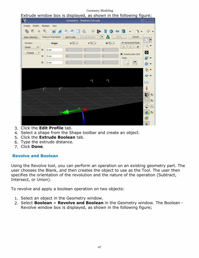
Extrude window box is displayed, as shown in the following figure;

Click the Edit Profile tab.3.Select a shape from the Shape toolbar and create an object.4.Click the Extrude Boolean tab.5.Type the extrude distance.6.Click Done.7.

Revolve and Boolean

Using the Revolve tool, you can perform an operation on an existing geometry part. Theuser chooses the Blank, and then creates the object to use as the Tool. The user thenspecifies the orientation of the revolution and the nature of the operation (Subtract,Intersect, or Union).

To revolve and apply a boolean operation on two objects:

Select an object in the Geometry window.1.Select Boolean > Revolve and Boolean in the Geometry window. The Boolean -2.Revolve window box is displayed, as shown in the following figure;

Geometry Modeling

48

Click the Edit Profile tab.3.Select a shape from the Shape toolbar and create an object.4.Click the Revolve tab.5.Type the angle.6.Click Done.7.

Holes may also be extruded or revolved through any part with its respective tool in thismenu. An object is selected in the Pick Blank tab and the cross section of the hole issketched and oriented in the Edit Profile and Feature Orientation tabs. Then, the shape ofthe removed section is specified in the Extrude Boolean tab, or Revolve tab depending onwhich operation is selected. The Preview tab shows a preview of the object before thechanges are formally applied to the project. For more information on defining extrusionsor revolutions, refer to 3-D Solid Modeling Options (geometry). An image of each booleanoperation is available in Boolean Operations (geometry).

Creating Patterns

Patterns are created by replicating a single selected object multiple times in one of theorganized arrangements listed below:

Geometry Modeling

49

Linear patternCylindrical patternHex-cylindrical patternSpherical patternElliptical pattern hex patternRadial patternPolar grid pattern

NoteFor the definitions and images associated with these patterns, refer to 3-D Patterns (geometry).

Geometry Modeling

50

Using Geometry Modeling ToolsIn this section, you will learn how to use the geometric modeling tools available in EMPro.

Shapes

Edge tools

Edge tools are used to create lines of various shapes within the EMPro interface. Thefollowing figure displays the Edge Tools including the Straight Edge tool (upper left),Polyline Edge tool (upper right), Tangent Line tool (lower left) and Perpendicular Edge tool(lower right).

Pressing |Tab| while using these tools will bring up the Specify Position dialog, which is used to enterrelevant properties to the tool being used.

The Edge Tools

Straight Edge

Creates a simple straight edge. To use this tool, click the Straight Edge button and clicktwo points in the sketching plane where the endpoints should be located.

Polyline Edge

The Polyline Edge is similar to the Straight Edge tool except it allows multiple points to

Geometry Modeling

51

create a series of connected straight edges. Click a starting point in the sketching planeand continue clicking on the locations of subsequent endpoints to create desired polylineedge. Click on the first vertex or press |Return| to finish.

Perpendicular Edge

Creates a straight edge perpendicular to an existing edge. To use, select the PerpendicularEdge button and click on the existing edge that will define the perpendicular direction.This can be a straight or curved edge. Then click on the location of the first and secondendpoints of the perpendicular straight edge.

Tangent Line

Similar to the Perpendicular Edge tool, but instead draws a line tangent to a pre-existing,non-linear edge. To use, select the Tangent Line tool, and click on the existing curve thatwill define the tangential direction. Then click on the location of the first and secondendpoints of the tangential straight edge.

Closed Polygon Tools

The following illustration displays the Closed Polygon tools including the Rectangle,Polygon and N-Sided Polygon tools.

The Closed Polygon tools

Rectangle

Creates a simple rectangle. Click the desired location of the first vertex of the rectangleand drag the mouse to the location of the second vertex.

Polygon

Creates a polygon specified by the user. (For regular polygons, see N-Sided Polygon). Itfunctions like the Polyline Edge tool. Click the starting point and all subsequent points,then press |Return| to close the polygon. This will draw a line from the last selectedendpoint to the first endpoint.

N-Sided Polygon

Geometry Modeling

52

Creates a regular, N-Sided Polygon of a user-specified number of sides. Click the locationof the center of the polygon. Then press the left-bracket key '[', or the right-bracket key']' to decrease or increase the number of sides, respectively. Once the correct number ofsides is selected, drag the mouse until the desired size and orientation around the centerpoint is achieved and click again to finish the N-sided polygon.

Arc Tools

The figure below displays two of the arc tools: the 3-Point Arc and 2-Point Arc tools.

The Arc tools

3-Point Arc Tool

Creates an open arc from three points. Click on the location of the first endpoint. Click asecond location to specify a point between the two endpoints (which helps determinesize), and a third location to specify the other endpoint.

2-point Arc Tool

Creates a semi-circle from two points. Click on the first endpoint location and drag themouse until the desired semi-circle size and orientation is achieved. Click this second endpoint location to finish.

Arc center, 2 points Tool

Creates an open arc from three points. First, click on the location of the center of the arc.Secondly, click a point to specify the radius of the arc. Finally, click the location of theendpoint to specify the length of the arc.

Circle and Ellipse Tools

The following figure displays an example of a circle drawn with the Circle Center, Radiustool.

A circle drawn with Circle Center, Radius tool

Geometry Modeling

53

Circle Center, Radius

Creates a circle defined by its center point and radius. Click the location of the circle'scenter point, then select another point to define the radius and finish the circle.

3-point Circle

Creates a circle based on three user-specified points, similar to the 3-Point Arc tool. Clickthe first two points to set the location of the circle and the third to specify its size.

2-point Circle

Creates a circle based on the distance between two points. After selecting the first point,choose the second to define the diameter and finish the circle.

Ellipse

Draws an ellipse from three points: the center and two perpendicular radii. Click thecenter point of the ellipse, then select the desired location of the first radii. Finally, selectthe desired length of the second radii, perpendicular to the first.

Tools

Select/Manipulate

Selects anything within the sketch. This is the default tool when no other tool is selected.It can be used to:

Move an object, edge, or vertex to a new position, by clicking-and-draggingSelect a vertex or edge and lock or edit its position, by right-clicking and selectingLock Position or Edit Position.Edit the value of an angle or distance constraint, by right-clicking and selecting theedit option.Delete an edge or constraint, by right-clicking and selecting the delete option.

Select/Manipulate tool

Geometry Modeling

54

Trim Curves

Deletes segments of curves until they intersect with other curves. To use this tool, click onthe section of the curve that is to be deleted.

Trim Curves tool

Insert Vertex

Inserts a vertex onto an already existing edge. Click the desired location of the new vertexon the existing edge.

Insert Vertex tool

Fillet Vertex

Converts a sharp corner into a rounded corner between two curves. Click on any sharpcorner and drag until the desired fillet radius is achieved and click to finalize fillet.

Geometry Modeling

55

Fillet Vertex tool

Inspect Geometry

Right-click an object (or multiple objects) in the Parts list or Geometry window and selectthe Inspect Geometry command. The Geometry Inspector window is displayed, whichprovides information about the geometry quality of objects. It describes the geometryproblem that is associated with the selected object.

Constraints

The geometry Constraints tools are used to modify pre-drawn shapes to the desiredspecifications.

Some of the "before" images below have been marked with white arrows to show which edges areconstrained in the "after" image on the right.

Horizontal Constraint

Constrains a segment to the horizontal direction.

Polygon before (left) and after (right) two sides are constrained horizontally

Vertical Constraint

Constrains a segment to the vertical direction.

Polygon before (left) and after (right) two sides are vertically constrained

Geometry Modeling

56

Collinear Constraint

Constrains two straight segments so that they are in line with each other.

Polygon before (left) and after (right) after two sides are constrained to be collinear

Parallel Constraint

Constrains two straight segments so that they are parallel to each other.

Polygon before (left) and after (right) two sides are constrained in parallel

Perpendicular Constraint

Constrains two straight segments so that they are perpendicular to each other. The

Geometry Modeling

57

following figure displays a polygon before (left) and after (right) two sides areperpendicularly constrained

Tangent Constraint

Constrains a straight segment so that it is tangent to a circular segment at a point. In thefollowing figure, Circle and polygon before (left) and after (right) a side of the polygon isconstrained tangentially with reference to the circle:

Concentric Constraint

Constrains two circular segments so that they are centered upon the same point. In thefollowing figure, two circles before (left) and after (right) are made concentric:

Angle Constraint

Geometry Modeling

58

Constrains an angle to a user-specified value between two straight lines. Click once toselect angle, then click a second time to place label and enter the angle size. In the figurebelow, the polygon before (left) and after (right) an angle has been constrained to a user-defined value.

Distance Constraint

Constrains the distance between two points, the distance between a point and a line, orthe length of a line to a user-specified value. After selecting the object(s) to constrain,click a final time to place label and enter distance.

As shown in the figure below, there are three different constraint "modes": parallel,vertical and horizontal. The mode is determined by the location of the mouse cursor whenyou click to specify where the constraint should be drawn.

Geometry Modeling

59

The polygon (A) before line has been constrained, (B) with a parallel distance constraint,(C) with a vertical distance constraint and (D) with a horizontal distance constraint.

Equal Length Constraint

Constrains selected segments to an equal length (assumes the length of the segmentselected second). Polygon before (left) and after (right) two sides are made equal lengthto one another.

Equal Distance Constraint

Constrains two pairs of points so that each pair assumes a distance from each other equalto the distance between the original pair.In the following figure, polygon before (left) andafter (right) two sides are made equal distance from each other:

Geometry Modeling

60

Radius Constraint

Constrains the radius to a user-specified value.

Equal Radius Constraint

Constrains selected radii to an equal length. In the following figure, two Circles before(left) and after (right) their radii are made equal:

Snapping

Snapping tools are used to snap the mouse to a specific point or edge in the EMProgeometry.

The blue lines in the images below highlight the "snap-to" landmarks.

Snap to Grid Line

Mouse is snapped to the nearest point on the nearest grid line.

Snap to Grid Line Tool

Geometry Modeling

61

Snap to Grid/Edge Intersections

Mouse is snapped to the nearest intersection between the grid and the sketch edge.

Snap to Grid/Edge Intersections Tool

Snap to Vertices

Mouse is snapped to the nearest vertex of the sketch or edge mid-point within range.

Snap to Vertices Tool

Geometry Modeling

62

Snap to Edges

Mouse is snapped to the edges of a pre-defined object.

Snap to Edges Tool

Snap to Edge/Edge Intersections

Mouse is snapped to the vertices of intersecting edges.

Snap to Edge/Edge Intersection Tool

Geometry Modeling

63

2D Modeling Options

The 2D Modeling tools are used to outline or fill-in a simple geometry object.

Wire Body

The Wire Body tool is the simplest geometry object. Any of the Shape tools can be used tocreate the desired wire geometry.

Sheet Body

The Sheet Body tool is similar to the Wire Body tool except its interior is filled with amaterial.

It is also possible to create a sheet body using advanced options with 3D modeling operations.

Sheet Body from Faces

The Sheet Body from Faces tool enables you to create a Sheet Body from the face of apre-existing geometry object. The interface will prompt the user to select the desiredobject face.

3D Solid Modeling Options

The 3D Modeling tools are used to create simple solid geometry objects from 2D forms.

For solid body creation, the 2D sketch must be closed so that there are no lingering endpoints.

Extrude

Extrude is used to sweep a face in the normal direction from its center. Once a 2D form ismade in the Edit Cross Section tab, select the Extrude tab to its right to perform anextrusion. For a default extrusion, define the distance in the Extrude Distance dialog boxby typing in a numerical value, parameter name (See: Section Defining Parameters), orequation.

Geometry Modeling

64

If units are not entered next to the numerical value, the default units are assumed. For more informationabout defining distances with parameter names, refer to Defining Parameters.

Additionally, the Direction dialog box specifies the axis along which the extrusion willoccur. Clicking done after the desired geometry is created will add the object to theproject. It can now be seen in the Project Tree.

Extrusion Tool

Revolve

Revolve is used to sweep a face in a circular path. Once a 2D form in made in the EditCross Section tab, select the Revolve tab to perform a revolution. For a default revolution,define the angle in the Angle dialog box by typing in a numerical value, parameter name,or equation. The Axis Root Position dialog specifies the location of the root of the axisaround which the shape will revolve. The Axis Direction box specifies the direction alongwhich the revolution will occur. Clicking DONE after the desired geometry is created willadd the object to the project. It can now be seen in the Project Tree.

Revolution Tool

Geometry Modeling

65

Creating a sphere with the Revolution Tool

Advanced 3D Solid Modeling Operations

The Advanced 3D Modeling tools are used to modify a pre-defined 3D geometry object.They are available within the Extrude and Revolve operations.

Twist

Twist options control how much the face is twisted as it is swept. They can be specified byangle or law.

By Angle: Specify the total number of degrees that the face will twist while it is

Geometry Modeling

66

swept.By Law: Specify a mathematical expression to control the rate of twist as a functionof the variable X.In the following figure, the Twist Tool defined by A) Angle (90 degrees) and B) Law (

)

Draft Type

Draft Type options control the expansion or contraction of the edges of the face as it isswept from its initial position.

No Draft: No expansion or contraction of edges during sweep.Draft Angle: Specify the expansion or contraction angle from initial position.

A cylinder sweep with Draft By Angle (10 degrees)

Draft Law: Specify a mathematical law to control the shape of the sides as the face isswept from initial position as a function of the variable X.

A cylinder sweep with Draft By Law (.5sin(2x))

Geometry Modeling

67

End Distance/Start Distance: Specify the offset distance in the plane where the sweepends/begins.

A cylinder sweep with Draft By End Distance (1 mm) and Start Distance (1 mm)

Hole Draft Type

Hole Draft Type options control the expansion and contraction of a hole. They aretherefore only valid during sweeping operations applied to a faces that contain holes. HoleDraft Type can be defined based on the values assigned to the edges in Draft Typeoptions, or by angle.

No Draft: No expansion or contraction is applied to the hole, even if the face has aDraft Type applied to it.

Draft Angle: Specify the expansion or contraction angle from initial position.

Geometry Modeling

68

Hole with no Draft (left) and a defined Draft Angle (right)

With Periphery*: The expansion or contraction of the hole will be the same as theoutside edges of the face as specified in Draft Type.

Against Periphery: The expansion or contraction of the hole will be the opposite tothe outside edges of the face as specified in Draft Type. (i.e., the hole will contract asthe face expands and expand when the face contracts.)

Hole with Draft Angle against (left) and with the Periphery (right)

Gap Type Modeling Operations

The Gap Type specifies how to close the gap created by an offset. The default gap type isNatural, but the following options are available for filling gaps in the geometry.

Natural: Extends the two shapes along their natural curves until they intersect.Rounded: Creates a rounded corner between the two shapes.Extended: Draws two straight tangent lines from the ends of each shape until they

Geometry Modeling

69

intersect. Illustration of gap types, showing A) the original gap, B) Natural, C)Rounded and D) Extended.

Cut Off End

Controls the orientation of a face that does not follow its normal during a straightsweeping operation. Select this option to chop the end of the swept 3D object so that thenormal of the end face is aligned with the line used for sweeping. Original Model (Left) andModel After Cut Off End (Right).

Make Solid

This option makes the model entirely solid. If this option is not selected, the model will behollow.

Modifying Existing Geometry

Specify Orientation

The Specify Orientation button is used to position the selected geometry in the simulationspace.

For more information on using the Specify Orientation tab, refer to Specify Orientation Tab (geometry).For descriptions of the tools used to rotate, translate and zoom into the simulation space View Tools.

Chamfer Edges

Chamfer Edges operation creates a beveled edge between two surfaces. After selecting

Geometry Modeling

70

the edge, it will be trimmed at a 45 angle if Constant Distance is selected in the SpecifyDistance tab. Otherwise, the user enters the chamfer distance for the surfaces on the leftand right sides of the edge.

A Chamfer operation applied to a cylinder edge

Blend Edges

The Blend Edges operation rounds the selected edge of the geometry. Under the SpecifyRadius_tab, the user can enter the _Blend Radius to adjust the rounding factor.

A Blend operation applied to a cylinder edge

Shell Faces

The Shell Faces operation creates a shell from existing geometry. After selecting the facesto keep open, the user can enter the Shell Thickness under the Specify Thickness tab.

By definition, the shell operation is used on geometry which is intended to have volume. This operation isnot for use an object such as a Sheet Body, whose volume is insignificant in the EMPro calculation.

A Shell operation applied to a cylinder

Geometry Modeling

71

Loft Faces

The Loft Faces operation connects two parts of an existing geometry. Under the SpecifyLoft tab, the user can adjust the Smoothness Factor to create the desired shape. In thefollowing figure, two objects within a geometry with faces selected (left) and laterconnected by a Loft (right).

Remove Faces

The Remove Faces operation removes a blend or chamfer that was previously applied to ageometry edge. This operation must be applied before the user can offset the length of anobject.

This operation is useful for modifying objects that have been imported from CAD files.

Offset Faces

Using Offset Faces, you can specify a positive or negative offset distance to increase ordecrease the length of the selected model, respectively. The following figure displays acylinder with an applied negative offset (left) and positive offset (right).

Geometry Modeling

72

Offset Sheet Edges

Using Offset Sheet Edges, you can select an edge(s) and specify the offset distance toincrease or decrease the length of the selected edge(s).

Boolean Operations

Two Parts Boolean Operation

You can perform Boolean options perform on two existing geometry parts. In each case,one object is identified as the Tool (the part used to perform the modification), and theother as the Blank (the part that is modified). There are three types of operations:

SubtractUnionIntersectChopExtrude and BooleanExtrude and Revolve

In a Subtract operation, the Tool is subtracted from the Blank. In the Intersect and Unionoperations, the part selected first is inconsequential. The following figure displays theoriginal two objects (Upper Left), objects after Boolean Union (Upper Right), objects afterBoolean Intersection (Lower Left) and objects after Boolean Subtraction (Lower Right).

Geometry Modeling

73

For more information, see Performing Boolean Operations (geometry).

Extrude Boolean Operation

The Extrude Boolean option performs an operation on an existing geometry part. In thiscase, the user chooses the Blank, and then creates the object to use as the TOOL. Theuser then specifies the orientation of the extrusion and the nature of the operation (Subtract, Intersect, or Union). In essence, this operation is a shortcut for the Two PartsBoolean operation.

A boolean extrude operation

Revolve Boolean Operation

The Revolve Boolean option performs an operation on an existing geometry part. The userchooses the Blank, and then creates the object to use as the Tool. The user then specifiesthe orientation of the revolution and the nature of the operation (Subtract, Intersect, orUnion).

A boolean revolve operation

Geometry Modeling

74

3D Patterns

Linear/Rectangular Pattern

The Linear/Rectangular Pattern option enables you to select a part in the geometry andreplicate it in a linear pattern. After selecting the part to modify, define the Spacing andNumber Of Instances in the U', V' and W' directions. Spacing refers to the distancebetween objects in the specified direction, and Number of Instances refers to the numberof objects in the specified direction. For example, if three cylinders are to be spaced at 2-mm intervals in the U'-direction, the Spacing in the U'-direction is 2 mm and the Numberof Instances in the U'-direction is 3. Additionally, the Stagger check-boxes apply a staggerin the specified direction at every other instance in that direction.

Spacing refers to the distance between each object's center point in the specified object. So, for example,if the spacing between two cylinders does not exceed the distance of the cylinder's diameter, the cylinderswill overlap.

A linear pattern applied to a cylinder

Geometry Modeling

75

Circular/Elliptical Pattern

The Circular/Elliptical Pattern option enables you to select a part in the geometry andreplicate it in a circular or elliptical pattern. After selecting the part to modify, navigate tothe Specify Circular/Elliptical Pattern tab and define the following fields:

Axis Point - specifies the position of the axisAxis Normal - specifies values to define the direction of the patternRoot Position (available in Elliptical Mode) - specifies a point (usually the center of apart) to use as the reference to replicate in the elliptical pattern.Major Axis (available in Elliptical Mode) - specifies the direction of the major axis.Pattern Options

Instances - specifies the number of objects in the patternAngle - specifies the angle across which the objects are patterned i.e., (180 means that objects are patterned across half of the ellipse)Ratio (available in Elliptical Mode) - specifies the ratio of the minor axis to themajor axis

An elliptical pattern applied to a small cylinder

Right-click an object (or multiple objects) in the parts tree or in the Geometry window andselect the Inspect Geometry command. The Geometry Inspector window is displayed,which provides information about the geometry quality. It describes the problem that isassociated with the selected object.

Geometry Modeling

76

Orienting Objects in the SimulationSpaceWithin the EMPro interface, there are three primary coordinate systems: Global,Reference, and Local. These coordinate systems are distinguished in the GUI as thefollowing reference forms:

Global coordinates: X, Y, and ZReference coordinates: U, V, and WLocal coordinates: U, V, and W

The Global coordinate system does not change throughout the course of a project, so itsorigin location and three primary axes always remain fixed. The 3-D orientation objectmarked with X, Y and Z in the lower left corner of the Geometry workspace windowrepresents the Global coordinate system. This set of orientation vectors is referred to asthe Global Triad.

Each object in the Parts tree, including Assemblies, have a Local Coordinate System. It isthe coordinate system in which the object is defined, sketches are drawn, primitives likeBoxes and Bondwires are positioned. Each editing session has a Specify Orientation tab toalter this system. The figure below shows the set of orientation vectors displayed in thistab, known as the Orientation Triad, and which visualizes the Local Coordinate System.Initially, when new parts are created, their Local coordinate system is identical to theirReference coordinate system.

Local coordinate systems are always defined in terms of a Reference coordinate system,which is nothing else that the Local coordinate system of the parent object, or the Globalcoordinate system if there’s no parent. Usually, the parent object is the Assembly in whichan part is contained. To see or modify the Reference coordinate system, you open theSpecify Orientation tab of the parent. In other words, you can view or modify the Localcoordinate system of the parent. When Reference coordinate systems are moved orrotated, all Local coordinate systems defined within also move and rotate. However, this iscomplicated by the use of geometry attached Anchor points and directions. The followingfigure displays the result of the Orientation Triad on the location and orientation of theLocal coordinate system.

The Orientation Triad is used to correctly orient objects within the simulation space, by

Geometry Modeling

77

specifying their Local Coordinate System. The center of the Orientation Triad is referred toas the Origin. The Origin can be defined manually by typing in its coordinates, or byclicking the intended origin in the simulation space with the Pick: Origin tool. It may alsobe manually shifted by clicking and dragging the directional axis vector of interest. Formore information about the Pick: Origin tool, refer to Alignment Tools.

Using the Specify Orientation Tab

The Specify Orientation tab in the Geometry workspace is available for positioning anyphysical object in the simulation space. This tab provides tools for translating, twisting androtating an object using three different coordinate systems. There are two primary modesthat are available within this tab: Basic Mode, the default mode which is sufficient undermost circumstances, and Advanced Mode, which has more powerful functionality. The Pickand Align drop-down menus available in each mode provide additional options fororienting objects.

Basic Mode

The next figure shows the Specify Orientation tab in Basic Mode. The Context controlswhether the Orientation Triad's position and orientation is cited in the Global or ReferenceCoordinate System. Notice that in this figure, the coordinates are all defined in terms of X,Y, and Z, denoting the Global Coordinate System.

The Specify Orientation tab in Basic Mode

The origin and orientation of the Orientation Triad can be adjusted in several ways withinBasic Mode. All of these methods are also available in Advanced Mode.

The Origin coordinates specify the location of the origin of the Orientation Triad. The origincan be updated manually, or can be adjusted by clicking and dragging on one of thecolored primary-axis vectors of the Triad. The location display will update automatically.

The orientation of the axes is defined by clicking the icon found next to any of the axisdefinitions. This will change the column from gray (read-only) to white, so that the valuesin the column can be edited. The orientation may also be adjusted by right-clicking theaxis and choosing the appropriate tool in the context menu, displayed below.

Customizing the orientation of the simulation space

Geometry Modeling

78

Rotate By - rotates the coordinate system about the chosen axis.Translate By - prompts the user to type in a translation distance along the selectedaxis (analogous to clicking and dragging on the axis vector).Pick New Direction - redefines the direction of the selected axis in a new directionspecified by the user. This tool is also useful to align the selected axis with thesurface of other objects in the simulation space.

NoteClicking a point in the simulation space will assign the direction vector directly into the space. Thus,adjusting the view with the View buttons may facilitate this assignment.

Pick Two Points - aligns the axis to the direction of the vector between two user-selected points.Point At - redirects the selected axis by directing the vector from its origin to a user-selected point.

Clicking the Adavanced Mode in the Basic Mode dialog window will bring up the AdvancedMode window.

Alignment Tools

Direction Picking Tools

The Direction Picking Tools menu provides six tools for defining the location and directionof the Orientation Triad. In the descriptions of tools used to align one object to another,reference object refers to the pre-existing, stationary object used as a reference for thealignment, and "object to align" refers to the object that is to be aligned to the referenceobject using the respective tool.

Simple Plane

Select a plane on a reference object to orient the plane of the object to align. The normalvector will be directed out of (orthogonal to) the selected plane, as shown in the figurebelow. EMPro will adjust the object to align so that its face is aligned with the selectedplane of the reference object. Press the |Space| key until the object is correctly oriented.

Aligning a new object with an existing reference plane

Geometry Modeling

79

Origin

Select a point anywhere in the simulation space to position the origin of the OrientationTriad. (The normal vectors will not change orientation.)

Normal

This tool enables you to adjust the direction of the normal vector of the Orientation Triadwhile maintaining the same origin point. The normal direction can be defined by clicking apoint in the simulation space, in which case the W' - normal vector will be positioneddirectly into the simulation space. The normal vector can also be aligned with the face of areference object by holding the mouse over one of its faces, and the normal vector of theobject to align will be aligned with this face of interest.

It is convenient to use the View buttons to position the simulation space so that thisplacement achieves the desired orientation.Additionally, you can select |Space| to reverse the direction of the orientation vectorbefore placing it.

Direction for Twist

Twisting about an axis is performed by defining a normal vector. The object will be twistedabout the origin as the twist slider is moved left and right. The figure below shows theplacement of the normal (purple arrow) and the radius of twist about the origin.

Twisting an object about the origin

Geometry Modeling

80

Axis for Rotation

Unlike the Direction For Twist, the Axis For Rotation moves the object and OrientationTriad about a user-defined axis. The object will not be twisted as it is rotated (i.e., a faceoriginally faced in the Z -direction will always face in that direction independent of itsdisplacement).The figure below shows the rotation of the Orientation Triad and objectabout the user-defined axis (shown as a purple arrow).

Rotating an object about a user-defined axis

Axis for Rotation and Twist

This tool is analogous to the Axis For Rotation tool except when the object is rotatedaround the picked axis, it will also be twisted.

Align menu

The Align menu provides several tools for aligning features of a new object with those ona reference object.

Align Face Normals

Geometry Modeling

81

This tool aligns the face normal of the object to align with the normal of the referenceobject. Pick the face on the object to align, then pick the face of the reference object. Thetwo normal vectors will be used to orient the coordinate system such that the normalvectors are pointing toward each other or away from each other. The following figureshows an object to align (left) being aligned with a face on the reference object (right).The bottom image shows the two objects after they have been aligned.

Select |Space| to reverse the direction of the orientation vector before placing it.

Aligning two face normals

Match Points

This tool matches a user-selected point on the object to align with a user-selected pointon the reference object. Select a point on the object to align and select a second point onthe reference object. The following figure shows the original objects in the next figureafter two of their corners were matched.

Aligning points on objects

Geometry Modeling

82

Match Faces

This tool functions much like the Match Points tool above except that it aligns the normalsof two objects rather than discrete points. Select the object to align, then select the faceof the reference object. The two positions will be used to translate the first part such thatthe two selected points are coincident. Since aligning the faces of two objects do not giveregard to the placement of the moved object, it is often useful to slide the moved objectalong an axis on the Orientation Triad until the desired placement is achieved.

Press |Space| to reverse the direction of the orientation vector before placing it.

Advanced Mode

The options available in Advanced Mode enable you to manipulate virtually all aspects ofthe orientation of the coordinate system. The three main areas for editing in this mode,Anchor, Axis, and Twist, are located on the left of the editing window. Within each of thesethree areas are also definitions for Translations and Rotations, which are additional offsetsto the geometry within the defined coordinate system.

Translations can also be applied manually in any direction within the Translation definition.A translation will not affect the location of the anchor point, only the location of theOrientation Triad and attached object. It is important to be aware of which of the threecoordinate systems is selected in the Context definition when applying a manualtranslation, since it may affect the proper placement of the geometry.

Similarly, rotations may also be manually defined within the Rotation definition. Therotation, across the angle specified within Angle, will be applied to the Orientation Triad(and attached object) at the anchor point, in the direction specified by the U', V', and W'definitions. For example, defining: U' = 0 V' = 0 W' = 1

Geometry Modeling

83

Angle = "PI rad"

The Anchor will be rotated Π radians about the W' axis. If the definitions were changed to:

U' = 1 V' = 0 W' = 1 Angle = "PI rad"

then U' and W' will be automatically adjusted to U' = "0.707107" and W' = "0.707107",since the resulting rotation will rotate the orientation 0.707107 radians in the U' and W'directions.

The net movement of the Orientation Triad in the coordinate system will be:

U + U' + U'rotation V + V' + V'rotation W + W' + W'rotation

The Anchor, Axis, and Twist buttons are detailed below.

Orienting the Anchor

The following figure shows the Anchor editing dialog within Advanced Mode.

Modifying the location and orientation of the anchor

The anchor point is represented by a blue dot in the simulation space. It remains in placeregardless of rotations and translations that are applied to the Orientation Triad. Whenthis dialog is first opened, U, V, and W within the Anchor: Fixed Position section representthe location of the anchor point in the Reference Coordinate System. Adjusting thelocation of the anchor point will adjust the location of the Orientation Triad as well(although moving the Orientation Triad will NOT affect the position of the anchor point).

Orienting the Axis

The next figure shows the Axis editing dialog within Advanced Mode.

Modifying the orientation of the axis

Geometry Modeling

84

The Axis dialog controls the orientation of the axes of the anchor. The default orientationof the Orientation Triad vectors are:

U': U = 0 V': V = 0 W': W = 1

These can be redefined to assume any orientation. Changing the orientation of one axiswill automatically adjust the orientation of the other two axes, since they must alwaysexist at 90 degrees from one another.

The Define drop-down list enables you to specify which axis is associated with thedirection defined in the U, V, and W orientation boxes.

Twisting the Axis

The twist axis defines a second direction for orthogonalizing the triad. The next figureshows Twist editing dialog within Advanced Mode.

Twist dialog

Using the Picking and Detach Tool

The Picking Tool and Detach Tool buttons enable you to use the mouse to select an anchorpoint, axis location, or twist location, or to detach an anchor, axis location, or twistlocation (if defined), respectively. If you select the Detach button, FDTD removes theanchor point, axis location, or twist location from the reference geometry it is associatedwith. This change removes the connection between the objects. For example, when twoobjects are anchored together they will both move if the orientation of either objectchanges. If the anchor is removed, a change in orientation to one object will no longeraffect the second object. The Picking Tool is always active. However, the Detach Tool isactive only when an anchor point, axis direction, or twist direction is defined using thereference geometry.

Geometry Modeling

85

The Picking and Detach tools for the Anchor, Axis and Twist areas operate independentlybased on the radio button selected in the Specify Orientation Tab (Anchor, Axis, Twist).For example, if the Axis radio button is selected, the Picking Tool will enable you to placean axis on an object and the Detach Tool (if active) will enable you to detach the existingaxis from an object. You cannot select or detach any existing anchor points or twistdirections when the Axis radio button is selected, only Axes.

Anchor is a position, axis and twist are directions. Therefore, depending on which of theradio buttons is active you'll be doing a different thing. When you're picking a position youonly see a dot and you can choose a position on a line, vertex or face. When you'repicking the axis or twist you're defining a direction relative to other existing geometry.You'll see an arrow to show you which direction will be picked. When picking a position ordirection you have extra options available which can be seen by mousing over existinggeometry. Depending on what the mouse is over a different tooltip will appear telling youwhat actions are available. You can cycle through directions using space. Both positionand direction have the ability lock to a part or hide a part. Picking a position can center ona face or use the bounding box.

Orienting 2-D Sketches on the Sketching Plane

The correct placement of the Orientation Triad in relation to its corresponding parts iscritical to some 3-D modeling operations, especially during revolution and sweepingoperations. It is important to understand the functionality of the Orientation Triad inrelation to the operation that is performed. The following two examples show how theOrientation Triad should be placed about a 2-D cross section.

Orienting Sketches for Revolutions

The following illustrations demonstrate the placement of the Orientation Triad during arevolution operation. The first illustration shows a simple 2-D cross section sketched in theEdit Cross Section tab. Notice that the sketch does not intersect any of the primary axes.

NoteIt is important that the 2-D sketch does not touch any axis of revolution, or else the revolution cannot beperformed.

The next figure shows the revolution of the circle about the V' -axis, after which we seethe revolution of the circle in the U' - and V' -directions. Finally, in the last illustration wesee how the revolution operation is used to create a hollow, or solid sphere from an openor closed semi-circle cross section, respectively.

Orienting a 2-D cross section about an axis of revolution is displayed in the followingfigure:

Geometry Modeling

86

Cross section revolved about the V' -axis is displayed in the following figure:

Cross section revolved about the U' - and V' -axes is displayed in the following figure:

Geometry Modeling

87

Using (A.) open (hollow) and (B.) closed (solid) cross sections to (C.) create a sphere withthe Revolution operation is displayed in the following figure:

Geometry Modeling

88

MaterialsMaterials Overview (geometry)Selecting a Material (geometry)Assigning Materials to Objects (geometry)

Geometry Modeling

89

Materials OverviewEMPro enables you to define a variety of materials, including perfect metals, lossy metals,dielectric and anisotropic materials, semiconductors, and resistors. Once these materialdefinitions are entered, they can then be applied to geometric objects. The materials airand perfect metal are already defined for you. You can enter material definitions either inthe global material list, which is available to all projects, or in the project material list,which is available only for the current project. You can use the Material list in the Projecttree to:

Define materials.Add materials to a specific project.Assign materials to objects.

After creating objects and orienting them in the simulation space, you need to assignmaterial definitions to make a valid project. The Material Editor window is the maininterface used for defining materials. The series of tabbed windows within this window areused to define a material based on its constitutive parameters. After adding materials tothe project, you can drag and drop the material on the required geometry to apply it tothat object.

Material Properties of Object Surfaces

The material that makes up an object and the material that is on the surface of an objectdoes not have to be the same. You change the characteristics of the surface of an objectusing Boundaries.

Selecting a Material

The following types of electrical and magnetic material are available in EMPro:

FreespacePerfect ConductorIsotropicDiagonally AnisotropicAnisotropic (Electric only)

Although frequency-independent materials require the least memory during FDTDsimulations, there are some cases in which frequency-independent materials are notappropriate. Frequency-dependent or dispersive materials should be used in theseinstances. Some common examples of frequency-dependent materials are high watercontent materials such as human tissues, and metals excited at optical frequencies. EMProhas the capability of simulating electric and magnetic Debye and Drude materials such asplasmas, Lorentz materials, and anisotropic magnetic ferrites, as well as frequency-independent anisotropic dielectrics and nonlinear diagonally anisotropic dielectrics. Theseadditional sub-types are specified within the Isotropic, Diagonally Anisotropic andAnisotropic definitions.

FDTD is capable of simulating a wide variety of electric and magnetic materials. The most

Geometry Modeling

90

basic material of course is free space. All FDTD cells are initialized as free space and thefields at all cell edges are updated using the free space equations unless another materialis added to replace the free space.

Perfectly conducting electric and magnetic materials are simulated by setting the electricor magnetic field to zero for any cell edges located within these materials. Because of thesimplicity of the calculation for these materials, it is better to use a perfect conductorrather than a real conductor whenever feasible. Conductors such as copper can besimulated in FDTD, but since the equations for computing the fields in copper material aremore complicated than those for a perfect conductor, the calculation will take longer.Ofcourse for cases where only a small percentage of the FDTD cells are defined as aconductor, the difference in execution time will hardly be noticeable.

Frequency independent dielectric and magnetic materials, considered “normal” materialsby XFdtd, are defined by their constitutive parameters of relative permittivity andconductivity for the electrical material, or relative permeability and magnetic conductivityfor the magnetic material. In most cases, even when performing a broadband calculation,these materials are appropriate since the parameters do not vary significantly over thefrequency range.

In some cases a frequency independent material is not appropriate and instead afrequency dependent, or dispersive, material should be substituted. Some commonexamples of frequency dependent materials are high water content materials such ashuman tissues, and metals when excited at optical frequencies. Included in XFdtd is thecapability to simulate electric and magnetic Debye and Drude materials such as plasmas,Lorentz materials, and anisotropic magnetic ferrites, as well as frequency independentanisotropic dielectrics, and nonlinear diagonally anisotropic dielectrics.

Geometry Modeling

91

Selecting a MaterialFreespace is the most basic material definition. Every other type of material is includedwithin the Physical definition, Electric and Magnetic types should be assigned in theirrespective drop-down lists. There are five electrical and magnetic material types availablein EMPro:

FreespacePerfect ConductorIsotropicDiagonally AnisotropicAnisotropic (Electric only)

Although frequency-independent materials require the least memory during FDTDsimulations, there are some cases in which frequency-independent materials are notappropriate. Frequency-dependent or dispersive materials should be used in theseinstances. Some common examples of frequency-dependent materials are high watercontent materials such as human tissues, and metals excited at optical frequencies. EMProhas the capability of simulating electric and magnetic Debye and Drude materials such asplasmas, Lorentz materials, and anisotropic magnetic ferrites, as well as frequency-independent anisotropic dielectrics and nonlinear diagonally anisotropic dielectrics. Theseadditional sub-types are specified within the Isotropic, Diagonally Anisotropic andAnisotropic definitions.

The following sections will detail the various types of materials.

Freespace

Freespace is the most basic material. By default, the EMPro problem domain is initializedto free space. This material sets relative permittivity and permeability to one, andconductivities to zero.

The following figure shows the Material Editor when the Freespace material is defined.Notice that no Electric or Magnetic tab is available, since both are defined as Freespacematerial.

Defining a Freespace material

Geometry Modeling

92

Perfect Conductors

A Perfect Conductor has infinite conductivity and all fields found within it are zero. It hasthe same settings as the Freespace material, as seen in the figure above. It shouldtypically be used as an approximation when a good conductor is needed in anelectromagnetic calculation and losses aren't important. Attempting to include the effectsof a good conductor (rather than perfect conductor) may be difficult since the wavelengthinside the good conductor will become very small, requiring extremely small FDTD cells toprovide adequate sampling of the field values inside the material. This can, however, beovercome by checking the Surface Conductivity box in the Edit Material dialog box.

Electric Materials

Isotropic Materials

EMPro includes several Isotropic materials:

NondispersiveDebye/DrudeDjordjevicLorentzSampled (FDTD only)Nonlinear (FDTD only)

The next figure shows the Material Editor when an Isotropic material is defined. Note thatonly the Electric tab is available since Magnetic is defined as Freespace. If you defineMagnetic as another type, a Magnetic tab would be available as well.

Defining an Electric Material

Geometry Modeling

93

Nondispersive

Nondispersive material properties do not vary with frequency. The continuous-timeexpressions of Maxwell equations for linear, isotropic, and nondispersive materials whichwill be discretized in EMPro are:

and

where:

represents the electric permittivity,

represents the electric conductivity,

represents the magnetic permeability, and

represents the magnetic conductivity.

Defining a Nondispersive material

Geometry Modeling

94

The following types of methods exist for Isotropic Nondispersive materials:

Loss tangent

Substrate loss is traditionally modeled by the frequency independent imaginary part ofpermittivity via the loss tangent (TanD) parameter.

Here, Er is the real part of the complex permittivity.TanD is the loss tangent which should be >= 0.

Complex Permittivity

In EMPro the complex permittivity can also be entered directly, instead of using the losstangent.

ε=Er – jEi

where Ei =Er TanD. Since TanD >=0, Ei should also be >=0.

Note that ADS uses a different sign convention for the imaginary part of the complexpermittivity.In ADS ε=Er + jEi, where Ei = – Er.TanD. Since TanD >=0, Ei is <= 0 in ADS.

Index of refraction

The index of refraction, n, is the ratio between the speed of light in free space and thespeed of light in this material.

Geometry Modeling

95

c2=1/ε0µ0

v2=1/ε0ε0µ

where

c=speed of light in free spacev=speed of light in this materialε0=permittivity of free space

ε=relative permittivity of this materialµ0=permeability of free space

µ=relative permeability of this material

The index of refraction n is now defined as

n=c/v=sqrt(ε)

However, in EMPro the index of refraction only describes the electric material properties.

n=sqrt(ε)

and thus

ε =n2

Surface Resistance

The surface resistance of a material is the resistance of a strip for which the width is equalto the length.The law of Pouillet gives the resistance of a conductor as a function of the area and thelength.

R=ρl/A

whereR=resistance in Ωρ=resistivity in Ωml=length in mA=area in m2

For a metal strip the area is the product of thickness (t) and width (w)

A=tw

R=ρl/tw

When the strip is a square, the width and the length are equal (w=l), so that

Geometry Modeling

96

R=ρ/t

This is the surface resistance in Ω, typically expressed as Ω/Square.

The following figure displays the surface resistance options:

The surface resistance model is only supported for FEM simulations. The materialmodel is mostly useful for specifying losses on sheet objects and can be applied, forexample, on conductors where the thickness is much smaller compared to the widthof the conductor lines (e.g. smaller by a factor 10).

The (DC) loss is specified by the surface resistance per square where both the realand imaginary part can be specified. When the value Z_surface (ohms/square) isapplied to a sheet object with length L and width W, the total resistance of the sheetobject in the length direction is given by Z_surface*L/W.

Thickness Parameter

The thickness parameter T allows you to specify an equivalent thickness for the lossmodeling associated with the surface resistance model, and mainly influences how theskin effect is included in the model.

When applied to a sheet object:

Thickness parameter T = 0

Geometry Modeling

97

Correct DC loss modelNo skin effect model is included in the model.

Thickness parameter T≠ 0correct DC loss modelskin effect behavior equivalent to that of a 3D object with a thickness T andconductivity of 1/(Z_surface*T)

When applied to a 3D object

Thickness parameter T = 0NOT RECOMMENDEDThe DC model is incorrect and no skin effect is applied

Thickness parameter T ≠ 0DC value is correct only if T corresponds to the actual thickness of the 3D objectskin effect behavior equivalent to that of a 3D object with a thickness T andconductivity of 1/(Z_surface*T)

Debye/Drude

For a Debye/Drude material, the electrical Conductivity ( ) in , Infinite Frequency

Relative Permittivity , Number Of Poles, Static Relative Permittivity , and RelaxationTime ( ) in seconds must be specified. For a Debye material, must equal zero. A non-zero conductivity value results in a Drude material.

NoteThis is discussed in detail in Chapter 8 of the Kunz and Leubbers text, refer to Bibliography (geometry).

Defining a Debye/Drude material

Geometry Modeling

98

These parameters cannot be set arbitrarily or instability can occur in FDTD simulations.One constraint is that the FDTD timestep must be small enough to accurately calculate thetransient behavior of the material. If the timestep is 3% of the relaxation time or smaller,the time variation of the material parameters should be sufficiently resolved. Typically, thetimestep is a very small fraction of the relaxation time. In order to be clear about thesigns in the following discussion, note that we are using the engineering time variation of:

and we are defining the complex permittivity as:

For the FDTD calculation to be stable, the imaginary (loss) part ( ) of the complexpermittivity, including the effect of the conductivity term, must be positive for allfrequencies from zero frequency to infinite frequency. This condition results in a passivematerial. If is negative, then the material has gain and FDTD simulations will becomeunstable as the field amplitudes grow.

NoteSee equation 8.29 of the Kunz and Leubbers text, refer to Bibliography (geometry).

For a Debye material ( ), stability is assured by setting to a larger value than

. In order to have realistic behavior at high frequencies, should be no less than oneand should not be much larger than one. Thus the condition for strictly Debye material tobe stable for FDTD simulations is:

> = 0

If the conductivity is not zero, then the material has Drude behavior. There are differentconditions that can be satisfied for the imaginary part of the complex permittivity to bepositive so that FDTD simulations produce stable results. If the static permittivity isgreater than the infinite frequency permittivity then the conductivity can have any positivevalue. This results in the simplest set of conditions for a stable Drude Material:

>

These conditions are, however, too restrictive to specify general Drude materials. The

Geometry Modeling

99

more general Drude conditions are:

If ( ),

then:

otherwise: 0

where is the Freespace Permittivity of 8.854e-12

NoteMore general conditions for Drude materials can be determined from the discussion in Chapter 8, Section3 of the Kunz and Leubbers text, refer to Bibliography (geometry).

EMPro supports Debye and Lorentz material properties that allows modeling of frequencydependent materials including FR4 and plasmas.

To define a new material, right-click Definitions > Materials branch of the Project Treeand select New Material Definition. A Material object will be added to this branch.Depending on the project preferences, the Material Editor window will appearautomatically. If not, simply double-click on this object to bring up the editor. Similarly,double-click any existing Material icon to edit an existing material within the MaterialEditor.

Debye/Drude

For a Debye/Drude material, the electrical Conductivity ( ) in siemens per meter, Infinite

Frequency Relative Permittivity ( ), Number Of Poles, Static Relative Permittivity ( ),and Relaxation Time ( ) in seconds must be specified. For a Debye material, mustequal zero. A non-zero conductivity value results in a Drude material.

Defining a Debye/Drude material

Geometry Modeling

100

Lorentz

For a Lorentz material, the electrical Conductivity ( ) in siemens per meter, Infinite

Frequency Relative Permittivity ( ), Static Relative Permittivity ( ), ResonantFrequency and Damping Coefficient must be specified.

Defining a Lorentz material

Djordjevic

A Djordjevic material is implemented in a number of substrate models to fulfill thecausality requirement. The Djordjevic material ensures causality by using the followingformula to describe the complex permittivity as a function of frequency:

Geometry Modeling

101

(2)

where fL and fH are the model parameters

is the permittivity value when frequency approaches infinity and a is a constant factor.These two parameters are calculated by EMPro from Er, TanD, FreqForEpsrTanD,LowFreqForTanD, and HighFreqForTanD, which are substrate model parameters enteredby the user. FreqForEpsrTanD is the frequency at which for given Er and TanD theequations (1) and (2) are equivalent. Specifically,

(3)In other words, FreqForEpsrTanD represents the frequency at which Er and TanD havebeen measured, given the fact that the permittivity is frequency dependent in the physicalworld.

Below is an example illustrating the permittivity profile and how it is related to substratemodel parameters. The horizontal axis in both plots is frequency (Hz).

Graph Shows Real Part of Permittivity

Geometry Modeling

102

Solid Plot Shows Imaginary Part of Permittivity. Dashed Plot Shows TanD.

The corresponding parameters are:

Er = 4.6TanD = 0.03FreqForEpsrTanD = 1 GHzHighFreqForTanD = 1 THzLowFreqForTanD = 1 kHz

Lorentz

Stability in Lorentz materials for FDTD simulations should be obtained as long as

Conductivity and the FDTD timestep is 3% of the relaxation time or less. The limitson the material parameters are:

> 0

> 0

Defining a Lorentz material

Sampled

This material enables you to enter multiple relative permittivities and conductivities at one

Geometry Modeling

103

time. It will behave like a nondispersive material when the calculation engine is called andthe Wideband Eval Frequency dictates what parameters to use.

NoteThis is not a dispersive material and will not automatically be converted to one.

Defining a Sampled material

Nonlinear

The relative permittivity of a nonlinear isotropic dielectric material satisfies:

Where:

is relative permittivity

E is instantaneous cell edge E-field

is static (low ) relative permittivity

is infinite relative permittivity

Geometry Modeling

104

is the E magnitude above which the material becomes non-linear

is a scaling term

, and are coefficients

NoteNonlinear materials are not supported in FEM simulations.

Defining a Nonlinear material

Diagonally Anisotropic

The definitions for a Diagonally Anisotropic are equivalent to those correspondingdefinitions detailed for Isotropic materials, except the definitions in each of the principledirections are independently specified.

Anisotropic

Frequency-independent Anisotropic materials are defined in EMPro by the relativepermittivity, , and Conductivity, , tensors.

Defining an Anisotropic material

Geometry Modeling

105

The parameters below Conductivity represent the terms of and the parameters belowPermittivity (Infinite Frequency) represent the terms of as follows:

The conductivity and permittivity for frequency-independent anisotropic dielectricmaterials are represented by and , unlike the equations for linear, non-dispersive,frequency-dependent, isotropic materials. These are used in the time-domain FDTDupdate equations in place of and :

Complex Permittivity

The value of complex permittivity may need to be calculated for some materials. The realpart of the complex permittivity may be used for the relative permittivity. The conductivitycan be calculated from the imaginary part of the complex permittivity by multiplying by adesired output frequency value (in radian frequency), as shown by:

Geometry Modeling

106

Loss Tangent

The loss tangent can be entered directly into EMPro when it is known, typically for gooddielectrics. The FDTD engine can calculate the conductivity as a function of frequencyusing:

Surface Conductivity Correction

The fields inside a good conductor decay exponentially with a decay rate given by the skindepth. In order to get accurate results for the fields inside a good conductor, it would beneccessary to generate a mesh that has a cell size that is smaller than the skin depth. Athigh frequencies, this would require very small cells and is thus computationallyexpensive. Both the FDTD and FEM simulators offer a choice to approximate the fieldsinside good conductors to reduce this expense. These choices are controlled by theSurface Conductivity Correction box. By default, the Surface Conductivity Correction boxis not selected.

In FDTD simulations, the default behavior is to model the fields inside conductors. Thisgives the proper loss modeling at low frequencies, but underestimates the losses at highfrequencies unless the FDTD grid creates small cell sizes along the inside surface of goodconductors. An accurate accounting of the high frequency losses can be obtained bychecking the Surface Conductivity Correction box and specifying a nominal frequencyabout which the calculated losses will be most accurate.

In FEM simulations, the default behavior is to not model the fields inside conductors.Instead, an approximate surface impedance model is used on the surface of conductors.This gives the correct loss modeling at high frequencies. It also gives the correct DClosses for conductors with a uniform cross section. Slightly more accurate DC and lowfrequency losses for structures of varying cross section can be obtained by checking theSurface Conductivity Correction box. However, this can significantly degrade the accuracyof the high frequency losses from FEM simulations.

The Evaluation Frequency parameter that appears with the Surface ConductivityCorrection box selected is ignored for FEM simulations.

Magnetic Materials

EMPro also includes several types of magnetic materials. Many of these materials aresimply the magnetic counterpart to the dielectrics described in Electric Materials. Allrestrictions noted in the Electric Materials section apply to their magnetic counterparts.

The figure below shows the Material Editor when a Magnetic Isotropic material is defined.Note that only the Magnetic tab is available since Electric is defined as Freespace. If

Geometry Modeling

107

Electric was defined as another type, a Electric tab would be available as well.

Defining a Magnetic material

Isotropic

Nondispersive

See Nondispersive in the Electric Materials section.

Debye/Drude.

See Debye/Drude in the Electric Materials section.

Magnetized Ferrites

The first parameter related to magnetized ferrites is the Applied Field, ( ). Enter its

value in units of . This number will be used to calculate the Larmor precession

frequency ( ),

where is the gyromagnetic ratio ( ).

Next, enter the Internal Magnetization ( ) in units of . This number is used to

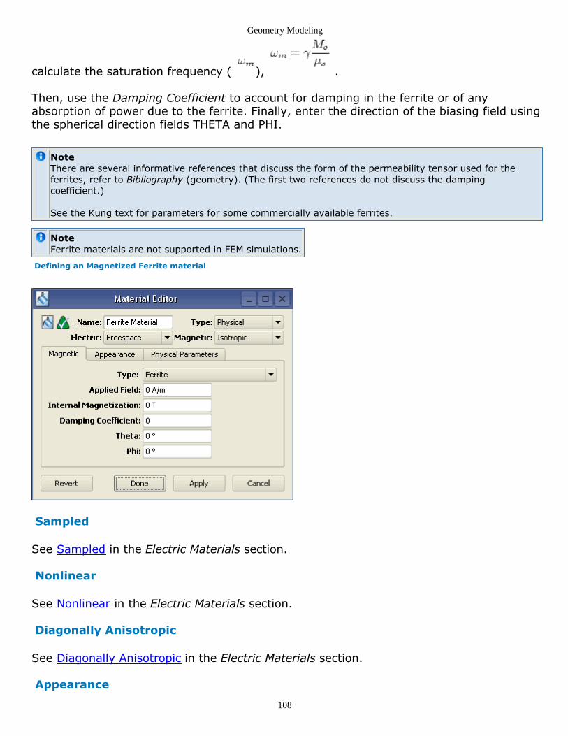
Geometry Modeling

108

calculate the saturation frequency ( ), .

Then, use the Damping Coefficient to account for damping in the ferrite or of anyabsorption of power due to the ferrite. Finally, enter the direction of the biasing field usingthe spherical direction fields THETA and PHI.

NoteThere are several informative references that discuss the form of the permeability tensor used for theferrites, refer to Bibliography (geometry). (The first two references do not discuss the dampingcoefficient.) See the Kung text for parameters for some commercially available ferrites.

NoteFerrite materials are not supported in FEM simulations.

Defining an Magnetized Ferrite material

Sampled

See Sampled in the Electric Materials section.

Nonlinear

See Nonlinear in the Electric Materials section.

Diagonally Anisotropic

See Diagonally Anisotropic in the Electric Materials section.

Appearance

Geometry Modeling

109

Use the Appearance tab to assign the aesthetic properties of each defined material. Colorsand other properties can be assigned to the faces, edges, and vertices of objects thatcontain the material so that they can be easily distinguished from other materials in theproject.

Physical Parameters

The Physical Parameters tab governs the definitions most commonly associated withbiological tissue. These definitions are thus necessary when performing biologicalcalculations. These values are computed automatically for tissues in Agilent Technologieshigh fidelity meshes.

Bibliography

K. S. Kunz and R. J. Luebbers, "The Finite Difference Time Domain Method for1.Electromagnetics". Upper Saddle River: CRC Press, 1993.A. Taflove and S. Hagness, Computational Electrodynamics: The Finite-Difference2.Time-Domain Method, Third Edition. New York: Artech House Publishers, 2005.C95.3-2002, "Recommended practice for measurements and computations of radio3.frequency electromagnetic fields with respect to human exposure to such fields,100khz to 300ghz," IEEE Standards and Coordinating Committee 28 on Non-IonizingRadiation Hazards, pp. i-126, April 2002.K. Yee, "Numerical solution of initial boundary value problems involving maxwell's4.equations in isotropic media," IEEE Transactions on Antennas and Propagation 14,pp. 302-307, 1966.C. Balanis, Advanced Engineering Electromagnetics. New York: Wiley, 1989. Section5.2.8.3.J. R. W. Simon Ramo and T. V. Duzer, Fields and Waves in Communication6.Electronics. New York: Wiley, 1994. Section 13.12.R. E. Collin, Foundations for Microwave Engineering. New York: Wiley-IEEE P, 2000.7.Section 6.7.B. Lax and K. J. Button, Microwave Ferrites and Ferrimagnetics. McGraw-Hill, 1962.8.Sections 4.1, 4.2.F. Kung and H. T. Chuah, "A finite-difference time-domain (fdtd) software for9.simulation of printed circuit board (pcb) assembly," Progress in ElectromagneticResearch, PIER 50, vol. Elsevier book series, pp. 299-335, 2005.D. M. Sheen, S. M. Ali, M. D. Abouzahra, and J. A. Kong, ``Application of the three-10.dimensional finite-difference time-domain method to the analysis of planar microstripcircuits,'' <EM>IEEE Transactions on Microwave Theory and Techniques</EM>,vol. 38, pp. 849-857, July 1990.

Geometry Modeling

110

Assigning Materials to ObjectsThere is no default material assigned to an object, you must assign material properties toeach object that is part of the simulated structure. You can assign either default materialsor create a new material.

For more information about type of materials, see Materials (geometry).

Assigning a Default Material

To add a default material:

Right-click Materials and choose the Select From Default Material Library1.option.Select a material from the Add a default material window.2.Click Add. The selected default material is added to the Material list.3.To assign a material, drag the material from Material list and drop it on the required4.object.

Adding a new material:

Right-click Materials in the Definitions list and select New Material Definition.1.Double-click the Material object to open the Material Editor window.2.Type a name of the new material in the Name text box.3.Define the Type of material as Physical or Freespace.4.

Specifying Priority

A default priority is assigned to the predefined materials and new materials that you candefine as user. If you assign a material to a 3D object, the object is assigned a defaultpriority from the material. However, you can change this object priority, which breaks thelink to the priority of the material. The following figure highlights the Priority field:

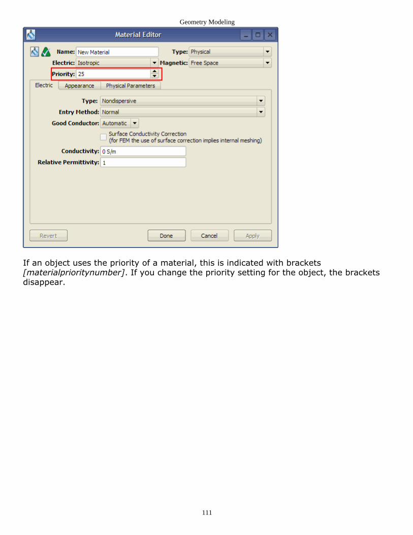
Geometry Modeling

111

If an object uses the priority of a material, this is indicated with brackets[materialprioritynumber]. If you change the priority setting for the object, the bracketsdisappear.