159
Ulrich Derenthal Geometry of universal torsors Dissertation

Ulrich Derenthal
Geometry ofuniversal torsors
Dissertation


Geometry of universal torsors
Dissertationzur Erlangung des Doktorgrades
der Mathematisch-Naturwissenschaftlichen Fakultatender Georg-August-Universitat zu Gottingen
vorgelegt von
Ulrich Derenthalaus
Brakel
Gottingen, 2006
D7Referent: Prof. Dr. Yuri TschinkelKorreferent: Prof. Dr. Victor BatyrevTag der mundlichen Prufung: 13. Oktober 2006

Preface
Many thanks are due to my advisor, Prof. Dr. Yuri Tschinkel, for intro-ducing me to the problems considered here and for his guidance.
I have benefitted from many discussions, especially with V. Batyrev,H.-C. Graf v. Bothmer, R. de la Breteche, T. D. Browning, B. Hassett,J. Hausen, D. R. Heath-Brown, J. Heinloth, M. Joyce, E. Peyre, and P.Salberger. I am grateful for their suggestions and advice.
Parts of this work were done while visiting the University of Oxford(March 2004), Rice University (February 2005), the CRM at Universite deMontreal (July 2005) during the special year on Analysis in Number Theory,the Courant Institute of Mathematical Sciences at New York University(December 2005), and the MSRI in Berkeley (March–May 2006) during theprogram Rational and Integral Points on Higher-Dimensional Varieties. Ithank these institutions for their support and ideal working conditions.
Calculations leading to some of my results were carried out on computersof the Gauss-Labor (Universitat Gottingen).
Financial support was provided by Studienstiftung des deutschen Volkesand DFG (Graduiertenkolleg Gruppen und Geometrie).
For proofreading, thanks go to Kristin Stroth and Robert Strich.I am grateful to my parents Anne-Marie and Josef Derenthal and my
sisters Birgitta and Kirstin for their support and encouragement. Finally,I thank Inga Kenter for the wonderful time during the last years.
Ulrich Derenthal
v


Contents
Preface v
Introduction 1
Part 1. Universal torsors of Del Pezzo surfaces 5
Chapter 1. Del Pezzo surfaces 71.1. Introduction 71.2. Blow-ups of smooth surfaces 81.3. Smooth Del Pezzo surfaces 111.4. Weyl groups and root systems 121.5. Singular Del Pezzo surfaces 151.6. Classification of singular Del Pezzo surfaces 171.7. Contracting (−1)-curves 201.8. Toric Del Pezzo surfaces 22
Chapter 2. Universal torsors and Cox rings 252.1. Introduction 252.2. Universal torsors 252.3. Cox rings 272.4. Generators and relations 27
Chapter 3. Cox rings of smooth Del Pezzo surfaces 313.1. Introduction 313.2. Relations in the Cox ring 313.3. Degree 3 343.4. Degree 2 383.5. Degree 1 40
Chapter 4. Universal torsors and homogeneous spaces 454.1. Introduction 454.2. Homogeneous spaces 474.3. Rescalings 504.4. Degree 3 534.5. Degree 2 55
Chapter 5. Universal torsors which are hypersurfaces 575.1. Introduction 575.2. Strategy of the proofs 585.3. Degree ≥ 6 615.4. Degree 5 635.5. Degree 4 66
vii

viii CONTENTS
5.6. Degree 3 73
Chapter 6. Cox rings of generalized Del Pezzo surfaces 816.1. Introduction 816.2. Generators 826.3. Relations 866.4. Degree 4 896.5. Degree 3 936.6. Families of Del Pezzo surfaces 96
Part 2. Rational points on Del Pezzo surfaces 99
Chapter 7. Manin’s conjecture 1017.1. Introduction 1017.2. Peyre’s constant 1057.3. Height zeta functions 106
Chapter 8. On a constant arising in Manin’s conjecture 1098.1. Introduction 1098.2. Smooth Del Pezzo surfaces 1118.3. Singular Del Pezzo surfaces 113
Chapter 9. Manin’s conjecture for a singular cubic surface 1179.1. Introduction 1179.2. Manin’s conjecture 1189.3. The universal torsor 1199.4. Congruences 1239.5. Summations 1249.6. Completion of the proof 129
Chapter 10. Manin’s conjecture for a singular quartic surface 13310.1. Introduction 13310.2. Geometric background 13410.3. Manin’s conjecture 13610.4. The universal torsor 13610.5. Summations 14010.6. Completion of the proof 144
Bibliography 145
Index 149
Lebenslauf 151

Introduction
The topic of this thesis is the geometry and arithmetic of Del Pezzosurfaces. Prime examples are cubic surfaces, which were already studiedby Cayley, Schlafli, Steiner, Clebsch, and Cremona in the 19th century.Many books and articles followed, for example by Segre [Seg42] and Manin[Man86].
On the geometric side, our main goal is to understand the geometry ofuniversal torsors over Del Pezzo surfaces. On the arithmetic side, we applyuniversal torsors to questions about rational points on Del Pezzo surfacesover number fields. We are concerned with the number of rational points ofbounded height in the context of Manin’s conjecture [FMT89].
More precisely, a smooth cubic surface S in three-dimensional projectivespace P3 over the field Q of rational numbers is defined by the vanishing ofa non-singular cubic form f ∈ Z[x0, x1, x2, x3]. Its rational points are
S(Q) := {x = (x0 : x1 : x2 : x3) ∈ P3(Q) | f(x) = 0}.
If S(Q) 6= ∅, then S(Q) is dense with respect to the Zariski topology, i.e.,there is no finite set of curves on S containing all rational points.
One natural approach to understand S(Q) is to ask how many rationalpoints of bounded height there are on S. Here, the height of a point x ∈ S(Q),represented by coprime integral coordinates x0, x1, x2, x3, is
H(x) := max{|x0|, |x1|, |x2|, |x3|}.
The number of rational points on S whose height is bounded by a positivenumber B is
NS,H(B) := #{x ∈ S(Q) | H(x) ≤ B}.
As it is difficult to determine the exact number NS,H(B), our question is:How does NS,H(B) behave asymptotically as B tends to infinity?
It is classically known that S contains 27 lines defined over the algebraicclosure of Q. If a line ` ⊂ S is rational, i.e., defined over Q, the numberof rational points on ` bounded by B behaves asymptotically as a non-zeroconstant multiple of B2. The behavior of NS,H(B) is dominated by therational points lying on rational lines, so we modify our question as follows:
Question. Let U be the complement of the lines on a smooth cubicsurface S. How does
NU,H(B) := #{x ∈ U(Q) | H(x) ≤ B}
behave asymptotically, as B →∞?
1
2 INTRODUCTION
The answer to this question depends on the geometry of S. Suppose thatS is split , i.e., all 27 lines on S are defined over Q. Then Manin’s conjecturalanswer is:
Conjecture. There is a positive constant c such that
NU,H(B) ∼ c ·B · (logB)6,
as B →∞.
This conjecture is open for smooth cubic surfaces. Analogous state-ments have been proved for some smooth Del Pezzo surfaces of degrees ≥ 5([BT98], [Bre02]).
An approach which is expected to lead to a proof of Manin’s conjecturefor Del Pezzo surfaces is the use of universal torsors. For the projectiveplane, this method is used as follows: In order to estimate the number ofrational points x ∈ P2(Q) whose height H(x) is bounded by B, we observethat these points are in bijection to the integral points
y = (y0, y1, y2) ∈ A3(Z) \ {(0, 0, 0)}
which satisfy the coprimality condition
gcd(y0, y1, y2) = 1
and the height condition
max{|y0|, |y1|, |y2|} ≤ B,
up to identification of y and −y. The number of these points y can beestimated using standard methods of analytic number theory.
There is a similar bijection between rational points of bounded heighton a cubic surface S and integral points on a certain affine variety TS , whichis called the universal torsor (see Chapter 2 for the definition), subject tocertain coprimality and height conditions.
We can establish such a bijection in two ways. On the one hand, thiscan be done by elementary transformations of the form f defining S such asintroducing new variables which are common divisors of previous coordinates(see Chapter 9 for an example). This way of passing to the universal torsorhas been used in the proof of Manin’s conjecture for some Del Pezzo surfacesof other degrees, e.g., [BB04]. We will see that these transformations aremotivated by the geometric structure of S.
On the other hand, we can compute universal torsors via Cox rings. ThePicard group Pic(S) of isomorphy classes of line bundles on S is an abeliangroup which is free of rank 7 if S is a split cubic surface. Effective linebundles have global sections, and the global sections of all isomorphy classesof line bundles on S can be given the structure of a ring, resulting in theCox ring Cox(S) (see Chapter 2). Its generators and relations correspond tothe coordinates and equations defining an affine variety A(S) which containsthe universal torsor TS as an open subset.
Batyrev and Popov [BP04] have determined the Cox ring of smoothDel Pezzo surfaces of degree ≥ 3. In the case of smooth cubic surfaces, thisrealizes the universal torsor as an open subset of a 9-dimensional variety,defined by 81 equations in 27-dimensional affine space (see Section 3.3).

INTRODUCTION 3
However, estimating the number of points on the universal torsor seems tobe very hard in this case.
Schlafli [Sch63] and Cayley [Cay69] classified singular cubic surfaces.For the cubic surface
S1 : x1x22 + x2x
20 + x3
3 = 0
with a singularity whose type is denoted as E6, Hassett and Tschinkel[HT04] have calculated the Cox ring. It is a polynomial ring in 10 variableswith one relation, resulting in a universal torsor which is a hypersurface in10-dimensional affine space. One of our main results is (see Theorem 9.1):
Theorem. Manin’s conjecture holds for the E6 cubic surface S1.
Joint work with de la Breteche and Browning resulting in a more preciseasymptotic formula for this surface will appear in [BBD05].
This thesis is organized in two parts. Part 1 is concerned with Cox ringsand universal torsors of smooth Del Pezzo surfaces and of generalized DelPezzo surfaces, i.e., minimal desingularizations of singular ones. We workover algebraically closed fields of characteristic 0. In Chapter 1, we givean exposition of the structure and classification of smooth, singular, andgeneralized Del Pezzo surfaces. In Chapter 2, we recall the definition ofuniversal torsors and Cox rings and collect some preliminary results on thegenerators and relations in the Cox ring of Del Pezzo surfaces.
Our main results concerning universal torsors and Cox rings of general-ized Del Pezzo surfaces are:
(1) We calculate the Cox ring of smooth cubic Del Pezzo surfaces ex-plicitly, using results of Batyrev and Popov [BP04] on the relationsup to radical in Cox(S) for smooth Del Pezzo surfaces of degree ≥ 3.We extend these results to surfaces of degree 2 and 1 (Theorem 3.2).
(2) We find all generalized Del Pezzo surfaces of degree ≥ 3 whoseuniversal torsor can be realized as a hypersurface in affine space, orequivalently, where the ideal of relations defining the Cox ring hasonly one generator (Theorem 5.1). We determine the Cox ring inthese cases.
(3) We give a method to determine generators and the ideal of relations(up to radical) of the Cox ring of any generalized Del Pezzo surfaceof degree ≥ 2 (Theorem 6.2 and Section 6.3).
Skorobogatov [Sko93] and Salberger observed that the universal torsorof a quintic Del Pezzo surface is an open subset of a Grassmannian.
Furthermore, for a smooth cubic surface S, the 27 coordinates of theaffine space containing the universal torsor correspond to the lines on S.Their classes in the Picard group can be identified with the weights of a 27-dimensional representation of the linear algebraic group associated to theroot system E6.
Batyrev conjectured that this is reflected geometrically by an embeddingof the universal torsor of S in a certain homogeneous space associated tothis representation, similar to the Grassmannian in the quintic case. Acorresponding result was proved by Popov [Pop01] in degree 4.

4 INTRODUCTION
(4) We prove Batyrev’s conjecture that universal torsors of smooth DelPezzo surfaces of degree 3 or 2 can be embedded naturally in theaffine cone over a homogeneous space associated to certain linearalgebraic groups (Theorem 4.1).
In Part 2, we apply our results of Part 1 to Manin’s conjecture forcertain Del Pezzo surfaces. In Chapter 7, we give a detailed introduction tothe usage of torsors towards Manin’s conjecture for Del Pezzo surfaces.
Our main results concerning Manin’s conjecture are:(5) We give a formula for a certain factor of the leading constant, as
proposed by Peyre [Pey95], in Manin’s conjecture for smooth andsingular Del Pezzo surfaces S. It is the volume of a polyhedronrelated to the cone of effective divisor classes on S. Our formulaallows to compute this constant directly from the degree and thetypes of singularities on S (Theorem 8.3 and Theorem 8.5).
(6) We prove Manin’s conjecture for a cubic surface with a singularityof type E6 (Theorem 9.1).
(7) We prove Manin’s conjecture for a split quartic surface with a sin-gularity of type D4 (Theorem 10.1).
Part 1
Universal torsors of Del Pezzosurfaces


CHAPTER 1
Del Pezzo surfaces
1.1. Introduction
This chapter gives an exposition of the structure and classification ofsmooth and singular Del Pezzo surfaces. For smooth Del Pezzo surfaces,a standard reference is [Man86], while [DP80] and [AN04] are modernaccounts of the structure and classification of singular Del Pezzo surfaces.
Schlafli [Sch63] and Cayley [Cay69] classified singular cubic surfacesin the 1860’s. Timms [Tim28] and Du Val [DV34] analyzed them moresystematically.
The basic objects of our studies are surfaces. For our purposes, theseare projective varieties of dimension 2 over a field K. In this chapter, weassume that the ground field K has characteristic zero and is algebraicallyclosed. For basic notions of algebraic geometry, we refer to Hartshorne’sbook [Har77].
We are mainly interested in the following geometric invariants of asmooth surface S:
Picard group: A prime divisor is an irreducible curve on S. Thefree abelian group generated by the prime divisors is the divisorgroup Div(S). Its elements are called divisors; non-negative linearcombinations of prime divisors are effective divisors. Consideringdivisors up to linear equivalence (cf. [Har77, Section II.6]) leadsto the Picard group Pic(S) of divisor classes as a quotient of thedivisor group.
Divisor classes correspond to line bundles, or invertible sheafs,on S; see [Har77, Section II.6] for details. We will freely go backand forth between these points of view; we will not distinguishbetween divisors and their classes whenever this cannot cause con-fusion.
Intersection form: For smooth prime divisors which intersect trans-versally, the intersection number is simply the number of intersec-tion points. This can be extended to a bilinear form on Div(S)and induces the intersection form (·, ·) on Pic(S) (cf. [Har77, Sec-tion V.1]). Let (D,D) be the self intersetion number of a divisor(class) D.
Canonical class: The canonical class KS of a smooth surface S, asdefined in [Har77, Section II.8], is the second exterior power ofthe sheaf of differentials on S. Its negative −KS is the anticanon-ical class. If S is a singular normal (see [Har77, Exercise 3.17])surface with rational double points (see [Art66]), we define its
7

8 1. DEL PEZZO SURFACES
anticanonical class −KS such that its pull-back under a minimaldesingularization f : S → S is −KeS .
Ampleness: A divisor class L ∈ Pic(S) is very ample if it definesan embedding of S in projective space (see [Har77, Section II.5]),while L′ ∈ Pic(S) is ample if a positive multiple of L′ is very ample.
Blow-ups: The blow-up of a point on a surface replaces this pointin a particular way by a divisor which has self intersection number−1 and which is isomorphic to the projective line P1 (cf. [Har77,Section I.4]).
In this chapter, we study the following classes of surfaces:• A smooth Del Pezzo surface is a smooth surface whose anticanonical
class is ample.• A singular Del Pezzo surface is a singular normal surface whose sin-
gularities are rational double points and whose anticanonical classis ample.
• A generalized Del Pezzo surface is either a smooth Del Pezzo surfaceor the minimal desingularization of a singular Del Pezzo surface.
The degree of a generalized Del Pezzo surface S is the self intersectionnumber of its anticanonical class. Generalized Del Pezzo surfaces of degree9− r ≤ 7 can be obtained by a sequence of r blow-ups of P2.
This chapter is structured as follows: In Section 1.2, we study howblow-ups affect basic invariants of surfaces such as the Picard group with itsintersection form and the anticanonical class. Section 1.3 is concerned withsmooth Del Pezzo surfaces and their prime divisors with self intersectionnumber −1, which we call (−1)-curves. In Section 1.4, we describe howcertain Weyl groups and root systems are connected to the configuration of(−1)-curves on smooth Del Pezzo surfaces.
Section 1.5 is concerned with singular and generalized Del Pezzo surfaces.The desingularization of singularities of singular Del Pezzo surfaces givesrise to prime divisors with self intersection number −2, which we call (−2)-curves. In Section 1.6, we show how the (−2)-curves of a generalized DelPezzo surface can be interpreted as the roots of root systems in the Picardgroup of a smooth Del Pezzo surface of the same degree, and how the (−1)-curves of these Del Pezzo surfaces are related. This allows the classificationof singular Del Pezzo surfaces. In Section 1.7, we explain how to recoverconfigurations of blown-up points from the configuration of (−1)- and (−2)-curves on generalized Del Pezzo surfaces. In Section 1.8, we determine whichgeneralized Del Pezzo surfaces are toric varieties [Ful93].
1.2. Blow-ups of smooth surfaces
A classical construction in algebraic geometry is the blow-up of a pointon a surface.
Lemma 1.1. Suppose S is a smooth surface. Let π : S′ → S be theblow-up of p ∈ S.
• The preimage E := π−1(p) is isomorphic to P1.• The map π is a birational morphism which is an isomorphism be-
tween S′ \ E and S \ {p}.
1.2. BLOW-UPS OF SMOOTH SURFACES 9
• The blow-up increases the rank of the Picard group by one:
Pic(S′) ∼= Pic(S)⊕ Z.
Here, E = (0, 1).• Let −KS be the anticanonical class on S. Then −KS′ = (−KS ,−1)
is the anticanonical class on S′.
In this context, we have the following terminology.• The curve E ⊂ S′ is called the exceptional divisor of the blow-upπ : S′ → S.
• For a prime divisor D on S, the strict (or proper) transform of DD is the prime divisor which is the closure of π−1(D \ {p}).
• Let α be the multiplicity of p ∈ S on the prime divisor D. Thetotal transform D′ of D is D′ := D + αE.
The canonical map π∗ : Pic(S) ↪→ Pic(S′) maps L ∈ Pic(S) to L′ = (L, 0).If L is the class of a divisor D, then L′ is the class of the total transform D′
of D. The class of the strict transform D of D is (L,−α).Whenever we use the same symbol for a divisor on a surface S and its
blow-up S′, it shall denote on S′ the strict transform of the divisor on S,unless specified differently.
Lemma 1.2. Let π : S′ → S be the blow-up of p ∈ S. Using the isomor-phism Pic(S′) ∼= Pic(S)⊕ Z as above, we have:
• The self intersection number of the exceptional divisor E is −1, andE does not intersect the total transforms of divisors on S.
• Let L1 = (M1, α1) and L2 = (M2, α2), where Li ∈ Pic(S′), Mi ∈Pic(S), αi ∈ Z. Then the intersection form on Pic(S′) is
(L1, L2) = (M1,M2)− α1 · α2.
• In particular, if the multiplicity of p on D is α, then (D, D) =(D,D)− α2, where D is the strict transform of D.
A prime divisor D with self intersection number (D,D) = n is called(n)-curve. A negative curve is an (n)-curve with n < 0. By Lemma 1.2,blowing up points creates negative curves. They have the following property.
Lemma 1.3. Let E be an effective divisor with negative self intersectionnumber. Then the space of global sections of the corresponding line bundleO(E) has dimension dimH0(S,O(E)) = 1.
Proof. Since E is effective, O(E) has global sections.Suppose dimH0(S,O(E)) ≥ 2. Then we can find two linearly indepen-
dent sections s1, s2. As (E,E) is the number of intersection points of theeffective divisors corresponding to s1 and s2, it must be non-negative. �
Therefore, the effective divisor corresponding to a divisor class with neg-ative self intersection number is unique.
Remark 1.4. As explained in [HT04, Section 3], the Picard group ispartially ordered : For L,L′ ∈ Pic(S), we have L � L′ if L′−L is an effectivedivisor class. If furthermore L 6= L′, we write L ≺ L′.
10 1. DEL PEZZO SURFACES
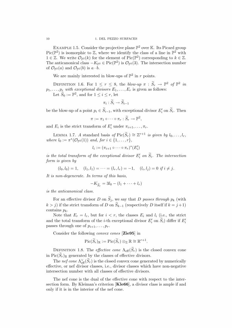
Example 1.5. Consider the projective plane P2 over K. Its Picard groupPic(P2) is isomorphic to Z, where we identify the class of a line in P2 with1 ∈ Z. We write OP2(k) for the element of Pic(P2) corresponding to k ∈ Z.The anticanonical class −KP2 ∈ Pic(P2) is OP2(3). The intersection numberof OP2(a) and OP2(b) is a · b.
We are mainly interested in blow-ups of P2 in r points.
Definition 1.6. For 1 ≤ r ≤ 8, the blow-up π : Sr → P2 of P2 inp1, . . . , pr with exceptional divisors E1, . . . , Er is given as follows:
Let S0 := P2, and for 1 ≤ i ≤ r, let
πi : Si → Si−1
be the blow-up of a point pi ∈ Si−1, with exceptional divisor E′i on Si. Then
π := π1 ◦ · · · ◦ πr : Sr → P2,
and Ei is the strict transform of E′i under πi+1, . . . , πr.
Lemma 1.7. A standard basis of Pic(Sr) ∼= Zr+1 is given by l0, . . . , lr,where l0 := π∗(OP2(1)) and, for i ∈ {1, . . . , r},
li := (πi+1 ◦ · · · ◦ πr)∗(E′i)
is the total transform of the exceptional divisor E′i on Si. The intersection
form is given by
(l0, l0) = 1, (l1, l1) = · · · = (lr, lr) = −1, (li, lj) = 0 if i 6= j.
It is non-degenerate. In terms of this basis,
−KeSr= 3l0 − (l1 + · · ·+ lr)
is the anticanonical class.
For an effective divisor D on Sj , we say that D passes through pk (withk > j) if the strict transform of D on Sk−1 (respectively D itself if k = j+1)contains pk.
Note that Er = lr, but for i < r, the classes Ei and li (i.e., the strictand the total transform of the i-th exceptional divisor E′
i on Si) differ if E′i
passes through one of pi+1, . . . , pr.
Consider the following convex cones [Zie95] in
Pic(Sr)R := Pic(Sr)⊗Z R ∼= Rr+1.
Definition 1.8. The effective cone Λeff(Sr) is the closed convex conein Pic(Sr)R generated by the classes of effective divisors.
The nef cone Λ∨eff(Sr) is the closed convex cone generated by numericallyeffective, or nef divisor classes, i.e., divisor classes which have non-negativeintersection number with all classes of effective divisors.
The nef cone is the dual of the effective cone with respect to the inter-section form. By Kleiman’s criterion [Kle66], a divisor class is ample if andonly if it is in the interior of the nef cone.

1.3. SMOOTH DEL PEZZO SURFACES 11
1.3. Smooth Del Pezzo surfaces
In this section, we describe basic properties of smooth Del Pezzo surfaces.
Definition 1.9. A smooth Del Pezzo surface is a smooth surface whoseanticanonical class is ample.
For 1 ≤ r ≤ 8, distinct points p1, . . . , pr in P2 are in general position if• there is no line in P2 containing three of them,• if r ≥ 6, no conic in P2 contains six of them,• if r = 8, no cubic curve in P2 containing all eight points has a
singularity in one of them.
Lemma 1.10. In the situation of Definition 1.6, the points p1, . . . , pr
are in general position if and only if every prime divisor D on Sr has selfintersection number (D,D) ≥ −1.
Proof. Consider how the self intersection numbers of prime divisors inP2 behave under blow-ups (Lemma 1.2). See also [DP80, Section II.3]. �
Theorem 1.11. A surface S is a smooth Del Pezzo surface if and onlyif S = P2, or S = P1 × P1, or S is the blow-up Sr of P2 in r ≤ 8 points ingeneral position. The degree is nine for P2, eight for P1 × P1, and 9− r forSr.
Proof. See [Man86, Theorem 24.4]. �
Remark 1.12. In the notation of Definition 1.6 and Lemma 1.7, thestrict and total transforms Ei and li of E′
i coincide if p1, . . . , pr are in generalposition. In this case, we usually use the notation Si := Si and H := l0, sothe standard basis is given by H,E1, . . . , Er.
If D ∈ Pic(S) is an effective divisor on a Del Pezzo surface S, then(−KS , D) > 0. By Lemma 1.10, the only negative curves on S are (−1)-curves. By [Man86, Theorem 24.3], we have (D,−KS) = 1 and D ∼= P1
exactly when D is a (−1)-curve. The proof uses the adjunction formula[Har77, Proposition V.1.5].
Remark 1.13. For r ≤ 6, the anticanonical class −KSr is φ∗r(OP9−r(1))for the anticanonical embedding
φr : Sr ↪→ P9−r.
The (−1)-curves on Sr are mapped exactly to the lines on φr(Sr) ⊂ P9−r.The image φ6(S6) of degree 3 in P3 is given by a non-singular cubic form,
while φ5(S5) of degree 4 in P4 is the intersection of two quadrics.
There are no (−1)-curves on the Del Pezzo surfaces P2 and P1 × P1.
Lemma 1.14. Let Sr be the blow-up of p1, . . . , pr ∈ P2 in general position.The (−1)-curves on Sr are the exceptional divisor E1, . . . , Er of the blow-upand the strict transforms of the following curves in P2:
• If r ≥ 2, the lines in P2 through two of the blown-up points.• If r ≥ 5, the conics through five of the blown-up points.• If r ≥ 7, the cubics through seven blown-up points, one of them a
double point of the cubic.
12 1. DEL PEZZO SURFACES
• If r = 8, the quartics through the eight points pi, three of themdouble points.
• If r = 8, the quintics through the eight points, six of them doublepoints.
• If r = 8, the sextics through the eight points, seven of them doubleand the eighth a triple point of the sextic.
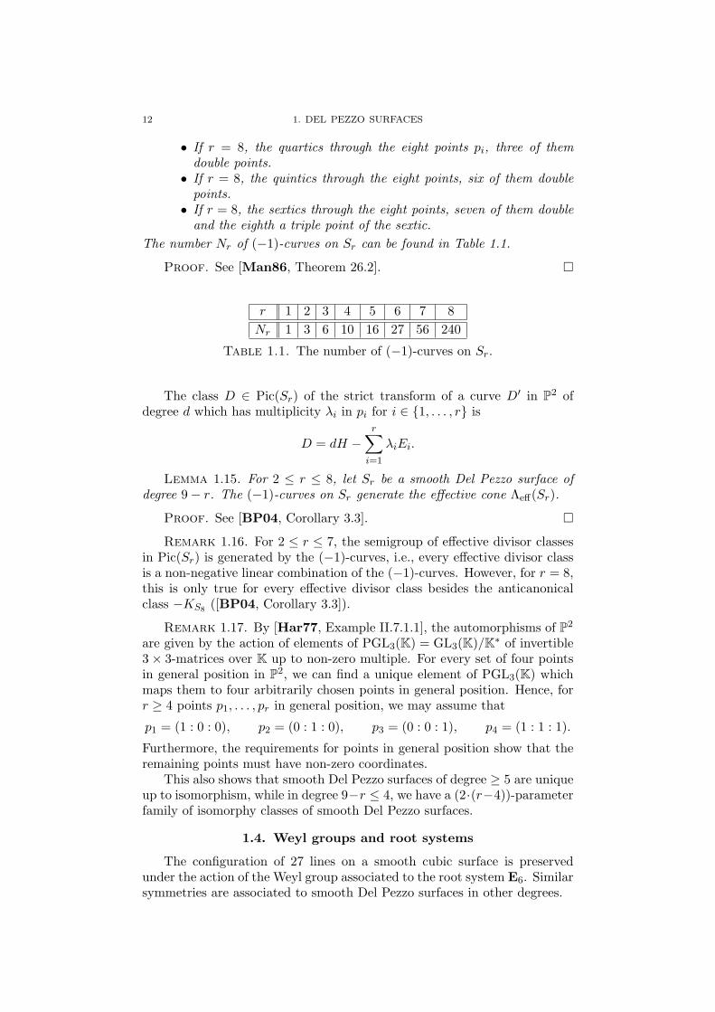
The number Nr of (−1)-curves on Sr can be found in Table 1.1.
Proof. See [Man86, Theorem 26.2]. �
r 1 2 3 4 5 6 7 8Nr 1 3 6 10 16 27 56 240
Table 1.1. The number of (−1)-curves on Sr.
The class D ∈ Pic(Sr) of the strict transform of a curve D′ in P2 ofdegree d which has multiplicity λi in pi for i ∈ {1, . . . , r} is
D = dH −r∑
i=1
λiEi.
Lemma 1.15. For 2 ≤ r ≤ 8, let Sr be a smooth Del Pezzo surface ofdegree 9− r. The (−1)-curves on Sr generate the effective cone Λeff(Sr).
Proof. See [BP04, Corollary 3.3]. �
Remark 1.16. For 2 ≤ r ≤ 7, the semigroup of effective divisor classesin Pic(Sr) is generated by the (−1)-curves, i.e., every effective divisor classis a non-negative linear combination of the (−1)-curves. However, for r = 8,this is only true for every effective divisor class besides the anticanonicalclass −KS8 ([BP04, Corollary 3.3]).
Remark 1.17. By [Har77, Example II.7.1.1], the automorphisms of P2
are given by the action of elements of PGL3(K) = GL3(K)/K∗ of invertible3× 3-matrices over K up to non-zero multiple. For every set of four pointsin general position in P2, we can find a unique element of PGL3(K) whichmaps them to four arbitrarily chosen points in general position. Hence, forr ≥ 4 points p1, . . . , pr in general position, we may assume that
p1 = (1 : 0 : 0), p2 = (0 : 1 : 0), p3 = (0 : 0 : 1), p4 = (1 : 1 : 1).
Furthermore, the requirements for points in general position show that theremaining points must have non-zero coordinates.
This also shows that smooth Del Pezzo surfaces of degree ≥ 5 are uniqueup to isomorphism, while in degree 9−r ≤ 4, we have a (2·(r−4))-parameterfamily of isomorphy classes of smooth Del Pezzo surfaces.
1.4. Weyl groups and root systems
The configuration of 27 lines on a smooth cubic surface is preservedunder the action of the Weyl group associated to the root system E6. Similarsymmetries are associated to smooth Del Pezzo surfaces in other degrees.
1.4. WEYL GROUPS AND ROOT SYSTEMS 13
Recall the definition of root systems and Weyl groups, for example from[Bro89]. Consider Rs with a non-degenerate bilinear form (·, ·). ForD ∈ Rs,let
D=k := {D′ ∈ Rs | (D′, D) = k}denote the hyperplane of elements of Rs whose pairing with D is k. Then
D≥k := {D′ ∈ Rs | (D′, D) ≥ k}
is the closed positive halfspace defined by D=k, while D>k := D≥k \D=k isthe open positive halfspace. Similarly, D≤k (resp. D<k) defines the closed(resp. open) negative halfspace.
A finite set Φ ⊂ Rs is a root system if it is invariant under the reflectionssα on α=0 for any α ∈ Φ, defined as
sα(x) := x− 2(x, α)(α, α)
· α.
The elements of Φ are called roots. The rank of Φ is the dimension of thesubspace of Rs which is generated by Φ.
For some D ∈ Rs such that D=0 ∩ Φ = ∅, let Φ+ = Φ ∩D>0 be the setof positive roots in Φ. For any α ∈ Φ, we have either α ∈ Φ+ or −α ∈ Φ+.Furthermore, we can find a minimal system ∆ of positive roots such thatany α ∈ Φ+ is a non-negative linear combination of elements of ∆. Theelements of ∆ are called simple roots. A root system Φ is represented bythe Dynkin diagram of its simple roots (see Remark 1.18).
The reflections sα for α ∈ Φ generate the finite Weyl group W whichacts on Rs. It acts transitively on Φ, and it is already generated by all sα
for α ∈ ∆.The hyperplanes α=0 for α ∈ Φ+ divide Rs into chambers (cf. [Bro89,
Section I.4B]). The (closed) fundamental chamber is
C0 := {x ∈ Rs | (x, α) ≥ 0 for all α ∈ ∆} =⋂
α∈∆
α≥0.
All other (closed) chambers have the form Cw := w(C0) for some w ∈ W .The set of chambers is in bijection to the set of elements of W . The spaceRs is the union of all chambers, and the dimension of the intersection of twochambers is smaller than s.
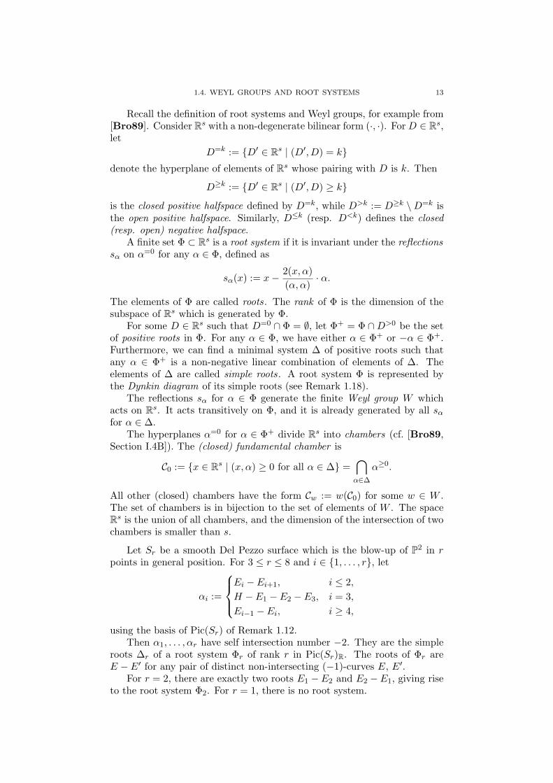
Let Sr be a smooth Del Pezzo surface which is the blow-up of P2 in rpoints in general position. For 3 ≤ r ≤ 8 and i ∈ {1, . . . , r}, let
αi :=
Ei − Ei+1, i ≤ 2,H − E1 − E2 − E3, i = 3,Ei−1 − Ei, i ≥ 4,
using the basis of Pic(Sr) of Remark 1.12.Then α1, . . . , αr have self intersection number −2. They are the simple
roots ∆r of a root system Φr of rank r in Pic(Sr)R. The roots of Φr areE − E′ for any pair of distinct non-intersecting (−1)-curves E, E′.
For r = 2, there are exactly two roots E1 −E2 and E2 −E1, giving riseto the root system Φ2. For r = 1, there is no root system.

14 1. DEL PEZZO SURFACES
Remark 1.18. We denote Dynkin diagram as follows. The symbols An,Dn, and En are associated to the following diagrams:
An (n ≥ 1) : GFED@ABCβ1 . . . GFED@ABCβn
Dn (n ≥ 4) : GFED@ABCβ1
GFED@ABCβ2GFED@ABCβ3 . . . GFED@ABCβn
En (6 ≤ n ≤ 8) : GFED@ABCβ3
GFED@ABCβ1GFED@ABCβ2
GFED@ABCβ4 . . . GFED@ABCβn
They contain n vertices corresponding to n simple roots β1, . . . , βn of anirreducible root system of rank n. The intersection number of two distinctsimple roots is the number of edges between the corresponding vertices; theself intersection number of a root is −2.
If a root system is the orthogonal sum of irreducible root systems, wedenote its type as a sum of the symbols corresponding to its irreduciblecomponents.
See Table 1.2 for the types of Φr.
r 2 3 4 5 6 7 8Φr A1 A2 + A1 A4 D5 E6 E7 E8
Table 1.2. Root systems associated to Sr.
For each root α ∈ Φr, the reflection sα is given by
sα(x) = x+ (x, α) · α,since (α, α) = −2. These reflections generate a Weyl group Wr. The inter-section form is invariant under the action of Wr. Therefore, Wr acts on theset of (−1)-curves on Sr. The anticanonical class −KSr is invariant underthis action.
Lemma 1.19. The Weyl group Wr acts transitively on the following sets:• The set of (−1)-curves on Sr, if r ≥ 3.• The set Φr of roots of Sr, if r ≥ 2.• The set of s-element sets of (−1)-curves which are pairwise non-
intersecting, if r ≥ 2 and s 6= r − 1.• The set of pairs of (−1)-curves which have intersection number 1,
if r ≥ 2.
Proof. For the first three statements, see [DP80, II, Theorem 2 andProposition 4]. The last statement follows from [FM02, Lemma 5.3] forr ≥ 4 (see also [BP04, Remark 4.7]). For r ∈ {2, 3}, we can check itdirectly. �
1.5. SINGULAR DEL PEZZO SURFACES 15
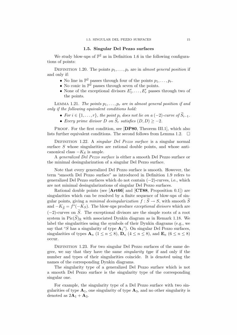
1.5. Singular Del Pezzo surfaces
We study blow-ups of P2 as in Definition 1.6 in the following configura-tions of points:
Definition 1.20. The points p1, . . . , pr are in almost general position ifand only if:
• No line in P2 passes through four of the points p1, . . . , pr.• No conic in P2 passes through seven of the points.• None of the exceptional divisors E′
1, . . . , E′r passes through two of
the points.
Lemma 1.21. The points p1, . . . , pr are in almost general position if andonly if the following equivalent conditions hold:
• For i ∈ {1, . . . , r}, the point pi does not lie on a (−2)-curve of Si−1.• Every prime divisor D on Sr satisfies (D,D) ≥ −2.
Proof. For the first condition, see [DP80, Theorem III.1], which alsolists further equivalent conditions. The second follows from Lemma 1.2. �
Definition 1.22. A singular Del Pezzo surface is a singular normalsurface S whose singularities are rational double points, and whose anti-canonical class −KS is ample.
A generalized Del Pezzo surface is either a smooth Del Pezzo surface orthe minimal desingularization of a singular Del Pezzo surface.
Note that every generalized Del Pezzo surface is smooth. However, theterm “smooth Del Pezzo surface” as introduced in Definition 1.9 refers togeneralized Del Pezzo surfaces which do not contain (−2)-curves, i.e., whichare not minimal desingularizations of singular Del Pezzo surfaces.
Rational double points (see [Art66] and [CT88, Proposition 0.1]) aresingularities which can be resolved by a finite sequence of blow-ups of sin-gular points, giving a minimal desingularization f : S → S, with smooth Sand −KeS = f∗(−KS). The blow-ups produce exceptional divisors which are(−2)-curves on S. The exceptional divisors are the simple roots of a rootsystem in Pic(S)R with associated Dynkin diagram as in Remark 1.18. Welabel the singularities using the symbols of their Dynkin diagrams (e.g., wesay that “S has a singularity of type A1”). On singular Del Pezzo surfaces,singularities of types An (1 ≤ n ≤ 8), Dn (4 ≤ n ≤ 8), and En (6 ≤ n ≤ 8)occur.
Definition 1.23. For two singular Del Pezzo surfaces of the same de-gree, we say that they have the same singularity type if and only if thenumber and types of their singularities coincide. It is denoted using thenames of the corresponding Dynkin diagrams.
The singularity type of a generalized Del Pezzo surface which is nota smooth Del Pezzo surface is the singularity type of the correspondingsingular one.
For example, the singularity type of a Del Pezzo surface with two sin-gularities of type A1, one singularity of type A3, and no other singularity isdenoted as 2A1 + A3.

16 1. DEL PEZZO SURFACES
Example 1.24. The Hirzebruch surface F2 := P(OP1 ⊕ OP1(−2)) is ageneralized Del Pezzo surface of degree 8 whose singularity type is A1. Formore details, see [Ful93, Section 1.1].
Theorem 1.25. Every generalized Del Pezzo surface is either P2, orP1 × P1, or the Hirzebruch surface F2, or the blow-up π : Sr → P2 in r ≤ 8points p1, . . . , pr in almost general position.
Proof. See [AN04]. �
If D ∈ Pic(S) is an effective divisor on a generalized Del Pezzo surfaceS, then (−KS , D) ≥ 0. A negative curve D fulfills D ∼= P1 and is either a(−1)-curve with (−KS , D) = 1, or a (−2)-curve with (−KS , D) = 0 by theadjunction formula. Furthermore, if (−KS , D) = 0 for a prime divisor D,then D is a (−2)-curve.
Let Sr be the blow-up of P2 in r points in almost general position. The(−2)-curves on Sr are the strict transforms of:
• the exceptional divisors E′1, . . . , E
′r which pass through one of the
points p1, . . . , pr,• if r ≥ 3, the lines in P2 which pass through three of p1, . . . , pr,• if r ≥ 6, the conics in P2 which pass through six of these points,• if r = 8, the cubics in P2 which pass through seven of these points,
with a singularity in the eighth.We will see in Proposition 8.11 that the effective cone of every generalized
Del Pezzo surface of degree ≤ 7 is generated by its negative curves.
Remark 1.26. For r ≤ 6, the anticanonical class −KSr of a singular DelPezzo surface Sr is φ∗r(OP9−r(1)) for the anticanonical embedding
φr : Sr ↪→ P9−r.
Let f : Sr → Sr be the minimal desingularization. Since −KeSr= f∗(−KSr),
the morphismφr ◦ f : Sr → P9−r
contracts exactly the (−2)-curves on Sr to the singularities of Sr and mapsthe (−1)-curves to the lines on the image of φr.
The image φ6(S6) of a singular cubic surface in P3 is given by a singularcubic form, while φ5(S5) of degree 4 in P4 is the intersection of two quadrics.
An important invariant of a generalized Del Pezzo surface is its extendedDynkin diagram, i.e., the configuration of the negative curves: We havea vertex for each negative curve, and the number of edges between twovertices is the intersection number of the corresponding negative curves. Inour diagrams, we mark the (−2)-curves using circles.
Example 1.27. By the classification of singular cubic surfaces [BW79],there is a unique cubic surface S6 with a singularity of type E6. Its anti-canonical embedding φ6(S6) ⊂ P3 is given by the vanishing of
f(x) = x1x22 + x2x
20 + x3
3.
It has one line {x2 = x3 = 0} containing the singularity (0 : 1 : 0 : 0). Itsminimal desingularization S6 contains six (−2)-curves E1, . . . , E6, and the
1.6. CLASSIFICATION OF SINGULAR DEL PEZZO SURFACES 17
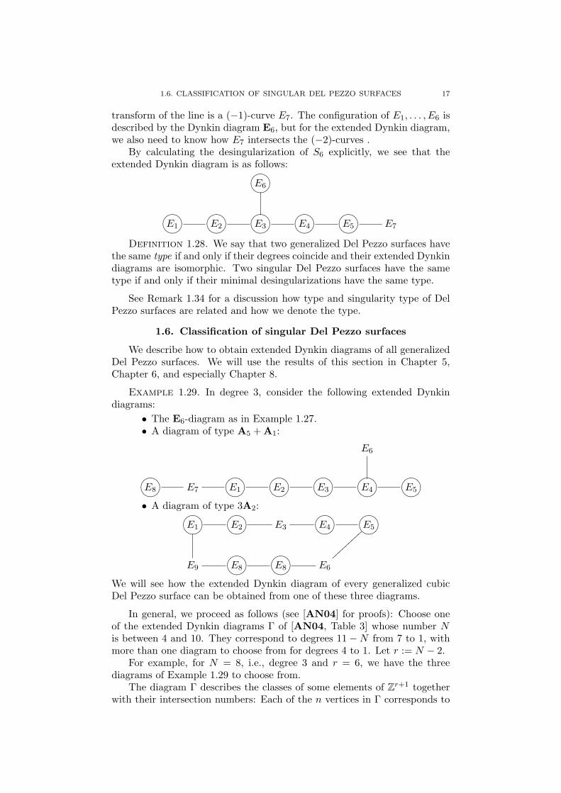
transform of the line is a (−1)-curve E7. The configuration of E1, . . . , E6 isdescribed by the Dynkin diagram E6, but for the extended Dynkin diagram,we also need to know how E7 intersects the (−2)-curves .
By calculating the desingularization of S6 explicitly, we see that theextended Dynkin diagram is as follows:
GFED@ABCE6
GFED@ABCE1GFED@ABCE2
GFED@ABCE3GFED@ABCE4
GFED@ABCE5 E7
Definition 1.28. We say that two generalized Del Pezzo surfaces havethe same type if and only if their degrees coincide and their extended Dynkindiagrams are isomorphic. Two singular Del Pezzo surfaces have the sametype if and only if their minimal desingularizations have the same type.
See Remark 1.34 for a discussion how type and singularity type of DelPezzo surfaces are related and how we denote the type.
1.6. Classification of singular Del Pezzo surfaces
We describe how to obtain extended Dynkin diagrams of all generalizedDel Pezzo surfaces. We will use the results of this section in Chapter 5,Chapter 6, and especially Chapter 8.
Example 1.29. In degree 3, consider the following extended Dynkindiagrams:
• The E6-diagram as in Example 1.27.• A diagram of type A5 + A1:
E6
GFED@ABCE8 E7GFED@ABCE1
GFED@ABCE2GFED@ABCE3
GFED@ABCE4GFED@ABCE5
• A diagram of type 3A2:
GFED@ABCE1GFED@ABCE2 E3
GFED@ABCE4GFED@ABCE5
E9GFED@ABCE8
GFED@ABCE8 E6
|||||||||
We will see how the extended Dynkin diagram of every generalized cubicDel Pezzo surface can be obtained from one of these three diagrams.
In general, we proceed as follows (see [AN04] for proofs): Choose oneof the extended Dynkin diagrams Γ of [AN04, Table 3] whose number Nis between 4 and 10. They correspond to degrees 11−N from 7 to 1, withmore than one diagram to choose from for degrees 4 to 1. Let r := N − 2.
For example, for N = 8, i.e., degree 3 and r = 6, we have the threediagrams of Example 1.29 to choose from.
The diagram Γ describes the classes of some elements of Zr+1 togetherwith their intersection numbers: Each of the n vertices in Γ corresponds to

18 1. DEL PEZZO SURFACES
a basis element ei of a lattice M :=⊕n
i=1 Zei with a bilinear form, where(ei, ei) = −2 if ei corresponds to a (−2)-curve in Γ (represented by a blackvertex in [AN04, Table 3], respectively marked by a circle in our notation),or (ei, ei) = −1 if ei corresponds to a (−1)-curve in Γ (represented by atransparent vertex, respectively without a circle), and (ei, ej) is the numberof edges between the corresponding vertices for i 6= j. This intersection formon M has rank r+1. Let K be the kernel of this form. Let Ei be the imageof ei in M/K ∼= Zr+1. The induced form (·, ·) on Zr+1 is a non-degeneratebilinear form, and the intersection behavior of E1, . . . , En is described by Γ.
The Ei with (Ei, Ei) = −2 form the simple roots ∆0 of a root systemΦ0 in Rr+1, generating a Weyl group W0. Let E0 be the set of Ei with selfintersection number −1.
Consider the orbit E of E0 ⊂ Zr+1 underW0: We can find an isomorphismZr+1 ∼= Pic(Sr) such that E is the set of (−1)-curves of Sr, and Φ0 is a rootsystem in Pic(Sr)R.
Remark 1.30. Note that W0 is equal to the Weyl group Wr associatedto the root system Φr listed in Table 1.2 only if we choose the first diagramin the list for N = r + 2 in [AN04, Table 3].
To construct the extended Dynkin diagram Γ(S) of the minimal desin-gularization S of a singular Del Pezzo surface S, choose a subset ∆ of ∆0.These are the simple roots of a root system Φ ⊂ Φ0, with positive rootsΦ+ ⊂ Φ+
0 . The reflections sα on the hyperplanes α=0 for the simple rootsα ∈ ∆ generate a Weyl group W ⊂ W0, with corresponding fundamentalchamber C0.
Theorem 1.31. For every choice of Γ from [AN04, Table 3] with N ∈{4, . . . , 10} (with corresponding simple roots ∆0 and (−1)-curves E), andevery choice of ∆ ⊂ ∆0 (giving a root system Φ with fundamental chamberC0), there is a generalized Del Pezzo surface S of degree 11−N whose (−2)-curves are ∆ and whose (−1)-curves are E ∩ C0.
The extended Dynkin diagram of every generalized Del Pezzo surface ofdegree ≤ 7 is obtained this way.
Proof. See [AN04]. �
Example 1.32. Consider the diagram of type A5 +A1 of Example 1.29corresponding to r = 6. This gives the following 8× 8 intersection matrix :
E1 E2 E3 E4 E5 E6 E7 E8
E1 −2 1 0 0 0 0 1 0E2 1 −2 1 0 0 0 0 0E3 0 1 −2 1 0 0 0 0E4 0 0 1 −2 1 1 0 0E5 0 0 0 1 −2 0 0 0E6 0 0 0 1 0 −1 0 0E7 1 0 0 0 0 0 −1 1E8 0 0 0 0 0 0 1 −2
We check that the rank of the intersection matrix is r + 1 = 7, and thatthe 7× 7 submatrix A of the first seven rows and columns has determinant
1.6. CLASSIFICATION OF SINGULAR DEL PEZZO SURFACES 19
with absolute value 1. Consequently, we can perform our computations inthe basis E1, . . . , E7, and E8 can be expressed in terms of this basis usingthe intersection numbers between E8 and E1, . . . , E7: As E8 intersects onlyE7, we have E8 = A−1 · (0, 0, 0, 0, 0, 0, 1) = (−1, 0, 1, 2, 1, 2,−2).
The elements E1, . . . , E5, E8 ∈ Z7 are the simple roots ∆0 of a rootsystem Φ0 of type A5 + A1. The reflections sEi on E=0
i for i ∈ {1, . . . , 5, 8}generate a Weyl group W0. The orbit E of E0 = {E6, E7} under W0 hasN6 = 27 elements. We can identify Z7 with Pic(S6) together with theintersection forms such that E is the set of (−1)-curves of a smooth cubicsurface S6, and Φ0 is a root system in Pic(S6). However, it is not thestandard root system Φ6 of type E6 associated to this configuration of 27(−1)-curves.
The Dynkin diagrams of various generalized Del Pezzo surfaces can beconstructed by choosing subsets ∆ of ∆0, for example:
• Let ∆ := ∆0. The (−1)-curves in the closed fundamental chamberC0 corresponding to ∆0 are exactly E0 = {E6, E7}. The extendedDynkin diagram of a generalized Del Pezzo surface S of type A5 +A1 is exactly the diagram Γ that we started with.
• Let ∆ := ∅. Then C0 is Pic(S6)R, and we obtain the diagram of asmooth cubic surface S6 containing 27 (−1)-curves.
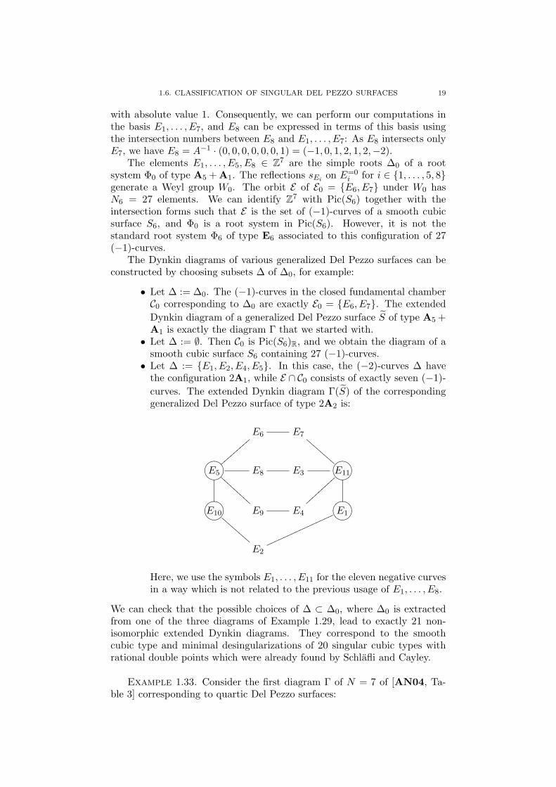
• Let ∆ := {E1, E2, E4, E5}. In this case, the (−2)-curves ∆ havethe configuration 2A1, while E ∩ C0 consists of exactly seven (−1)-curves. The extended Dynkin diagram Γ(S) of the correspondinggeneralized Del Pezzo surface of type 2A2 is:
E6 E7
CCCC
CCCC
GFED@ABCE5
{{{{{{{{{
BBBB
BBBB
B E8 E3GFED@ABCE11
GFED@ABCE10
CCCC
CCCC
E9 E4
||||||||| GFED@ABCE1
E2
nnnnnnnnnnnnnnnn
Here, we use the symbols E1, . . . , E11 for the eleven negative curvesin a way which is not related to the previous usage of E1, . . . , E8.
We can check that the possible choices of ∆ ⊂ ∆0, where ∆0 is extractedfrom one of the three diagrams of Example 1.29, lead to exactly 21 non-isomorphic extended Dynkin diagrams. They correspond to the smoothcubic type and minimal desingularizations of 20 singular cubic types withrational double points which were already found by Schlafli and Cayley.
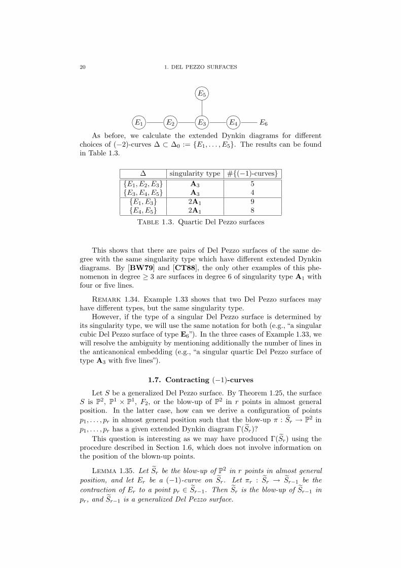
Example 1.33. Consider the first diagram Γ of N = 7 of [AN04, Ta-ble 3] corresponding to quartic Del Pezzo surfaces:
20 1. DEL PEZZO SURFACES
GFED@ABCE5
GFED@ABCE1GFED@ABCE2
GFED@ABCE3GFED@ABCE4 E6
As before, we calculate the extended Dynkin diagrams for differentchoices of (−2)-curves ∆ ⊂ ∆0 := {E1, . . . , E5}. The results can be foundin Table 1.3.
∆ singularity type #{(−1)-curves}{E1, E2, E3} A3 5{E3, E4, E5} A3 4{E1, E3} 2A1 9{E4, E5} 2A1 8
Table 1.3. Quartic Del Pezzo surfaces
This shows that there are pairs of Del Pezzo surfaces of the same de-gree with the same singularity type which have different extended Dynkindiagrams. By [BW79] and [CT88], the only other examples of this phe-nomenon in degree ≥ 3 are surfaces in degree 6 of singularity type A1 withfour or five lines.
Remark 1.34. Example 1.33 shows that two Del Pezzo surfaces mayhave different types, but the same singularity type.
However, if the type of a singular Del Pezzo surface is determined byits singularity type, we will use the same notation for both (e.g., “a singularcubic Del Pezzo surface of type E6”). In the three cases of Example 1.33, wewill resolve the ambiguity by mentioning additionally the number of lines inthe anticanonical embedding (e.g., “a singular quartic Del Pezzo surface oftype A3 with five lines”).
1.7. Contracting (−1)-curves
Let S be a generalized Del Pezzo surface. By Theorem 1.25, the surfaceS is P2, P1 × P1, F2, or the blow-up of P2 in r points in almost generalposition. In the latter case, how can we derive a configuration of pointsp1, . . . , pr in almost general position such that the blow-up π : Sr → P2 inp1, . . . , pr has a given extended Dynkin diagram Γ(Sr)?
This question is interesting as we may have produced Γ(Sr) using theprocedure described in Section 1.6, which does not involve information onthe position of the blown-up points.
Lemma 1.35. Let Sr be the blow-up of P2 in r points in almost generalposition, and let Er be a (−1)-curve on Sr. Let πr : Sr → Sr−1 be thecontraction of Er to a point pr ∈ Sr−1. Then Sr is the blow-up of Sr−1 inpr, and Sr−1 is a generalized Del Pezzo surface.

1.7. CONTRACTING (−1)-CURVES 21
Proof. As Sr is a blow-up of a smooth surface, there is at least one(−1)-curve on Sr. By Castelnuovo’s criterion [Har77, Theorem V.5.7], thecontraction of a (−1)-curve E on Sr to a point pr results in a smooth surfaceSr−1 such that Sr is the blow-up of Sr−1 in pr. By [DP80, Section III.9],Sr−1 is a generalized Del Pezzo surface. (Note that the Hirzebruch sur-face F2 was missed in [DP80, Section III.9], as mentioned after [CT88,Proposition 0.4].) �
In this situation, we can extract the intersection numbers (including selfintersection numbers) of the projections of the negative curves on Sr underπr. The only change is that the projections of curves which intersect Er
on Sr intersect pairwise on Sr−1 and have a higher self intersection number(Lemma 1.2). Every negative curve on Sr−1 is the projection of a negativecurve on Sr. This allows us to derive the extended Dynkin diagram of Sr−1.Furthermore, we learn which projections of the negative curves pass throughpr, giving some information on the position of the blown-up point.
The degree of Sr−1 is 9− (r − 1). If this is ≤ 7, i.e., r ≥ 3, then Sr−1 isthe blow-up of P2 in r− 1 points in almost general position. Therefore, anychoice of (−1)-curve E is suitable for a construction of Sr as the blow-up ofP2 in r points in almost general position.
On the other hand, if r = 2, then Γ(S2) is one of the following twodiagrams:
• Γ(S2,1) of a smooth Del Pezzo surface S2 = S2,1 of degree 7:
E1 E2 E3
• Γ(S2,2) of a Del Pezzo surface S2,2 of degree 7 and type A1:
GFED@ABCE1 E2 E3
Here, we must be careful with our choice of (−1)-curve, as in degree 8, only asmooth Del Pezzo surface S1 containing one (−1)-curve is the blow-up of P2.We must avoid P1 × P1 (containing no negative curves) and the Hirzebruchsurface F2 (containing one (−2)-curve).
The correct choice is to contract E1 or E3 in case of Γ(S2,1) (contract-ing E2 gives P1 × P1), and E2 in case of Γ(S2,2) (E1 is a (−2)-curve, andcontracting E3 gives F2) to obtain S1.
For r = 1, there is exactly one (−1)-curve on S1, which we contract toobtain π = π1 ◦ · · · ◦ πr : Sr → P2.
If a negative curve E on Sr is not contracted at any stage of this process,then π(E) is a curve in P2 whose self intersection number is the square ofits degree. Furthermore, we know the relative configuration of all π(E) andthe positions of the blown-up points pi relative to them. Of course, some ofthe blown-up points may lie on exceptional divisors of previous blow-ups.
Example 1.36. Consider the extended Dynkin diagram of the cubicsurface S6 of type 2A2 as constructed in Example 1.32 with negative curvesE1, . . . , E11. For i from 6 down to 1, the contraction
πi : Si → Si−1

22 1. DEL PEZZO SURFACES
maps the (−1)-curve Ei to the point pi ∈ Si−1, and the transform on Si−1
of a curve Ej on Si is also called Ej . We end up with S0 = P2. Letπ := π1 ◦ · · · ◦ π6. In more detail, this works as follows:
• Contracting E6 on S6 results in S5. The (−2)-curve E5 on S6 turnsinto a (−1)-curve on S5 and intersects E7, . . . , E10. The curve E7
on S5 has self intersection number 0.• Contracting E5 on S5 gives S4 on which E7, . . . , E10 intersect in
one point.• Contracting Ei on Si for i = 4, 3, 2, 1 results in S0 = P2 contain-
ing the curves E7, . . . , E11. Their self intersection numbers havechanged to 1, so they are lines in P2. While E7, . . . , E10 intersectin one point p ∈ P2, they are intersected by E11 away from p.
Reversing this process, the blown-up points p1, . . . , p6 are as follows:p1 = E10 ∩ E11, p2 = E1 ∩ E10, p3 = E8 ∩ E11,
p4 = E9 ∩ E11, p5 = E7 ∩ E8 ∩ E9 ∩ E10, p6 = E5 ∩ E7.
In terms of the standard basis (Lemma 1.7), E1, . . . , E11 are:E1 = l1 − l2, E2 = l2, E3 = l3, E4 = l4, E5 = l5 − l6,
E6 = l6, E7 = l0 − l5 − l6, E8 = l0 − l3 − l5, E9 = l0 − l4 − l5,
E10 = l0 − l1 − l2 − l5, E11 = l0 − l1 − l3 − l4.
The surface S6 is determined by the position of the lines E7, . . . , E11
in P2. Using automorphisms of P2 as in Remark 1.17, we may assumethat p = (1 : 0 : 0) in P2 = {(x0 : x1 : x2)}, while E11 = {x0 = 0}.Furthermore, we may assume that three of the four intersection points ofE11 with E7, . . . , E10 are at certain positions, while the choice of the fourthresults in a one-parameter family of generalized Del Pezzo surfaces of type2A2:
E7 = {x1 = 0}, E8 = {x2 = 0},E9 = {x1 − x2 = 0}, E10 = {x1 − αx2 = 0}.
(1.1)
The parameter α can take any value in K \ {0, 1}. In Section 6.6, we willreturn to this family of surfaces.
This example shows that there may be an infinite family of isomorphyclasses of cubic Del Pezzo surfaces of the same type. In other cases ofdegree 3, the number of isomorphy classes of a given type is finite:
• Type E6: Exactly one isomorphy class of cubic surfaces exists (seeExample 1.27).
• Type D4: Exactly two isomorphy classes exist (see [HT04, Re-mark 4.1]).
For singular cubic Del Pezzo surfaces, this and the number of parameters ineach infinite family can be found in [BW79].
1.8. Toric Del Pezzo surfaces
For an introduction to toric varieties, see [Ful93]. Toric surfaces areequivariant compactifications of a 2-dimensional torus T , for example P2,P1 × P1, and the Hirzebruch surface F2.

1.8. TORIC DEL PEZZO SURFACES 23
A toric surface contains divisors which are invariant under the actionof T . The T -invariant prime divisors intersect exactly in points which arefixed under T . In case of P2, the T -invariant prime divisors are three linesforming a triangle.
The blow-up of a toric variety is again toric if and only if we blow up apoint which is fixed under the action of T , i.e., an intersection point of twoT -invariant prime divisors D1, D2. The exceptional divisor E of the blow-upis T -invariant. Fixed points on E are exactly the intersection points of Ewith D1 and D2.
To construct toric generalised Del Pezzo surfaces other than P1 × P1
and F2, we blow up P2 in this way. Note that the only negative curvesare exceptional divisors and possibly the strict transforms of the three T -invariant lines on P2, i.e., a subset of all T -invariant prime divisors.
If we include all T -invariant prime divisors in the extended Dynkin di-agram, it has the shape of a “circle”. We denote it as a vector of self inter-section numbers. Two entries are next two each other (where we considerthe first and last entry as “next to each other”) if the corresponding primedivisors intersect. See Table 1.4 for the extended Dynkin diagrams of alltoric generalized Del Pezzo surfaces.
This result allows us to identify non-toric Del Pezzo surfaces from theirextended Dynkin diagrams: Whenever a negative curve intersects more thantwo other negative curves, the surface cannot be toric.
degree type extended Dynkin diagram9 P2 (1, 1, 1)8 smooth S1 (1, 0,−1, 0)
P1 × P1 (0, 0, 0, 0)F2 (−2, 0, 2, 0)
7 smooth S2 (0,−1,−1,−1, 0)A1 (1, 0,−2,−1,−1)
6 smooth S3 (−1,−1,−1,−1,−1,−1)A1 (4 lines) (0,−1,−1,−2,−1,−1)
2A1 (0,−2,−1,−2,−1, 0)A2 + A1 (1, 0,−2,−2,−1,−2)
5 2A1 (−1,−1,−1,−1,−2,−1,−2)A2 + A1 (0,−1,−1,−2,−2,−1,−2)
4 4A1 (−1,−2,−1,−2,−1,−2,−1,−2)A2 + 2A1 (−2,−1,−2,−1,−1,−2,−1,−2)A3 + 2A1 (0,−2,−1,−2,−2,−2,−1,−2)
3 3A2 (−2,−2,−1,−2,−2,−1,−2,−2,−1)
Table 1.4. Toric Del Pezzo surfaces.


CHAPTER 2
Universal torsors and Cox rings
2.1. Introduction
Universal torsors were introduced by Colliot-Thelene and Sansuc in con-nection with their studies of the Hasse principle for Del Pezzo surfaces ofdegrees 3 and 4 [CTS80], [CTS87]. We will see in Part 2 how they can beapplied to Manin’s conjecture.
Over an algebraically closed field K of characteristic 0, a universal torsorof a generalized Del Pezzo surface Sr of degree 9−r is constructed as follows:Let L0, . . . ,Lr be invertible sheaves whose classes form a basis of Pic(Sr).Let L◦i be the sheaf obtained by removing the zero section from Li. Thenthe bundle
TSr := L◦0 ×Sr · · · ×Sr L◦rover Sr is a universal torsor (see Lemma 2.3).
The Cox ring, or homogeneous coordinate ring, of Sr is the space
Cox(Sr) =⊕
(ν0,...,νr)∈Zr+1
H0(Sr,L⊗ν00 ⊗ · · · ⊗ L⊗νr
r )
whose ring structure is induced by the multiplication of global sections. Wewill see that TSr is an open subset of A(Sr) := Spec(Cox(Sr)).
This section has the following structure: In Section 2.2, we discuss uni-versal torsors over non-closed fields. In Section 2.3, we give basic propertiesof Cox rings. In Section 2.4, we collect some preliminary results on genera-tors of a Cox ring as a K-algebra and relations between these generators.
The following Chapters 3, 5, and 6 are concerned with the explicit deter-mination of generators and relations in Cox rings of generalized Del Pezzosurfaces.
2.2. Universal torsors
Over a field K of characteristic 0 with algebraic closure K, let S be asmooth projective surface, with geometric Picard group Pic(SK) ∼= Zr+1,where SK := S ×Spec K Spec K.
Let T be an algebraic torus, i.e., a linear algebraic group such that TKis isomorphic to Gs
m for some s ∈ Z>0. Let T be a variety with a faithfullyflat morphism π : T → S and an action of T on T . As explained in [Pey98,Section 3.3], T is called a T -torsor over S if and only if the natural mapT ×Spec K T → T ×S T is an isomorphism.
The T -torsors over S up to isomorphism are classified by the etale co-homology group H1
et(S, T ).
25

26 2. UNIVERSAL TORSORS AND COX RINGS
Proposition 2.1. For every p ∈ S(K), there is a T -torsor πp : Tp → S(unique up to isomorphism) such that p ∈ πp(Tp(K)).
If K is a number field, S(K) is the union of πpi(Tpi(K)) for a finite setof points p1, . . . , pn ∈ S(K).
Proof. We construct πp : Tp → S as follows (see [CTS80, Section II]):We have a map
S(K)×H1et(S, T ) → H1(K, T )
(p, [T ]) 7→ [T (p)],where T (p) := T ×S Spec K(p) is a K-form of T , with [T (p)] = 0 in theGalois cohomology group
H1(K, T ) = H1(Gal(K/K), T (K))
if and only if p ∈ π(T (K)). Using the map φ : H1(K, T ) → H1et(S, T ), we
can construct a torsor πp : Tp → S of the class [T ] − φ([T (p)]) ∈ H1et(S, T )
such that p ∈ πp(Tp).See [CTS80, Proposition 2] for the second statement. �
The Picard group Pic(SK) and the group of characters
X∗(T ) := Hom(TK,Gm)
of the torus T are free Z-modules with an action of Gal(K/K). By [CTS87,Section 2.2], there is a map
ρ : H1et(S, T ) → HomGal(K/K)(X
∗(T ),Pic(SK)),
defined by ρ([T ])(χ) := χ∗(T ) for any χ ∈ X∗(T ). Here, HomGal(K/K)(·, ·)denotes the homomorphisms of free Z-modules which are compatible withthe Gal(K/K)-action.
The torus TNS(S) := Hom(Pic(S),Gm) is called the Neron-Severi torusof S. If the ground field K is algebraically closed, it is isomorphic to Gr+1
m
after the choice of a basis of Pic(S). The group of characters X∗(TNS(S)) iscanonically isomorphic to Pic(SK).
Definition 2.2. A universal torsor TS over S as above is a TNS(S)-torsor such that ρ([TS ]) = idPic(SK).
Lemma 2.3. Let K be an algebraically closed field of characteristic 0.Let L0, . . . ,Lr be a basis of Pic(S). The bundle
T := L◦0 ×S · · · ×S L◦ris a universal torsor over S.
Proof. The isomorphism φ : Pic(SK) → X∗(TNS(S)) gives a basisχ0, . . . , χr of X∗(TNS(S)), with χi := φ(Li). By definition, ρ([T ])(χi) forthe character χi ∈ X∗(TNS(S)) is the class of (χi)∗(T ) in Pic(SK), which isLi as required. �
Over an algebraically closed field of characteristic 0, TS as defined inLemma 2.3 does not depend on the chosen basis of Pic(S) by [Pey04, Propo-sition 8]. In fact, every universal torsor is isomorphic to it.
Over non-closed fields K, the existence of a K-rational point p on Simplies the existence of a universal torsor π : TS → S, defined over K

2.4. GENERATORS AND RELATIONS 27
(Proposition 2.1). In this case, TS becomes isomorphic over K to T as inLemma 2.3. If S(K) = ∅, a universal torsor does not necessarily exist over K.
2.3. Cox rings
The following construction is due to [HK00], generalizing the homoge-neous coordinate ring of toric varieties in [Cox95].
As before, let L0, . . . ,Lr be a basis of Pic(S) ∼= Zr+1 for a smoothprojective surface S over an algebraically closed field K. Let H0(S,L) bethe K-vector space of global sections of L ∈ Pic(S), which we also denoteby H0(L).
For ν = (ν0, . . . , νr) ∈ Zr+1, let
Lν := L⊗ν00 ⊗ · · · ⊗ L⊗νr
r .
For ν,µ ∈ Zr+1, the multiplication of sections defines a map
H0(Lν)×H0(Lµ) → H0(Lν+µ).
Definition 2.4. For S and L0, . . . ,Lr as above, the Cox ring , or homo-geneous coordinate ring , of S is defined as
Cox(S) :=⊕
ν∈Zr+1
H0(Lν),
where the multiplication of sections
H0(Lν)×H0(Lµ) → H0(Lν+µ)
induces the multiplication in Cox(S).
For any algebra A with a Pic(S)-grading, we will denote the part ofdegree O(D) for a divisor D by AD or AO(D). We have a Pic(S)-grading onCox(S) as follows:
Cox(S)D = Cox(S)O(D) = H0(O(D)).
If Lν � Lµ in the partial ordering of Pic(S), multiplication by a non-zeroglobal section of Lµ−ν induces an inclusion
Cox(S)Lν ↪→ Cox(S)Lµ .
As remarked in [HK00, Section 2], the Cox ring of S is unique up toisomorphism. However, we cannot simply define it without the choice ofa basis of Pic(S) since the multiplication would be defined only up to aconstant.
2.4. Generators and relations
Let S be a generalized Del Pezzo surface over an algebraically closed fieldK of characteristic 0. A line bundle L ∈ Pic(S) has global sections if andonly if L is the class of an effective divisor. Therefore, the Pic(S)-degrees inwhich Cox(S) is non-zero lie in the effective cone Λeff(S) (Definition 1.8).
Lemma 2.5. The ring Cox(S) is a finitely generated K-algebra. Let Nbe the minimal number of generators of Cox(S).
• We can find a system of N generators which are homogeneous withrespect to the Pic(S)-grading.
28 2. UNIVERSAL TORSORS AND COX RINGS
• Up to permutation, the Pic(S)-degrees of a minimal system of ho-mogeneous generators are unique.
• Given any set of homogeneous generators, we can find a subset ofN elements which is a generating system.
Proof. The Cox ring is finitely generated by [HK00, Corollary 2.16and Proposition 2.9]. Note that we will also prove this in Theorem 6.2 if thedegree of S is ≥ 2. Since K is algebraically closed, Cox(S) is by definition thedirect sum of its homogeneous components. Hence, we can find a minimalsystem of generators containing only homogeneous elements.
We use the partial order on the effective divisor classes. Any homoge-neous expression involving an element of degree L′ ∈ Pic(S) has degree Lwith L′ � L. Consequently, Cox(S)L is generated by elements of degreeL′ � L.
Let C be the subalgebra of Cox(S) generated by all elements of degreeL′ ≺ L. For a system of homogeneous generators of Cox(S), the generatorsof degree L′ ≺ L generate exactly C since generators of degree L′′ 6≺ Lcannot affect the degrees L′ ≺ L. Therefore, we have at least
nL := dim(Cox(S)L)− dim(CL)
generators of degree L.Therefore, any system of homogeneous generators must contain at least
nL elements of degree L. If there are more than that for some L, we canremove an appropriate number of generators of degree L since we are simplylooking for a basis in the vector space Cox(S)L. �
Remark 2.6. Once any set of generators is known, we can find a minimalgenerating set: First, we replace each generator by its homogeneous parts.Then we go through the degrees L of these homogeneous generators in theirpartial ordering and check for each L whether we may remove some of thegenerators, as explained in the proof of Lemma 2.5.
We will see in the following chapters how to determine systems of gen-erators.
Lemma 2.7. If E is a negative curve on S, then every homogeneoussystem of generators of Cox(S) contains a section of degree E.
The number of generators of Cox(S) must be at least the number ofnegative curves.
Proof. By Lemma 1.3, the space H0(O(E)) is one-dimensional.If a non-zero global section s of O(E) can be expressed in terms of
homogeneous sections of other degrees, then O(E) must be a non-trivialnon-negative linear combination of other effective divisor classes. This wouldallow us to construct a section which is linearly independent of s. �
However, the example of the E6 cubic surface [HT04, Section 3] showsthat the Cox ring of a generalized Del Pezzo surface S can have other gener-ators besides sections of negative curves. In view of Lemma 1.15 and Propo-sition 8.11, the following result shows that the degrees of these generatorslie in the nef cone if the degree of S is ≤ 7.
2.4. GENERATORS AND RELATIONS 29
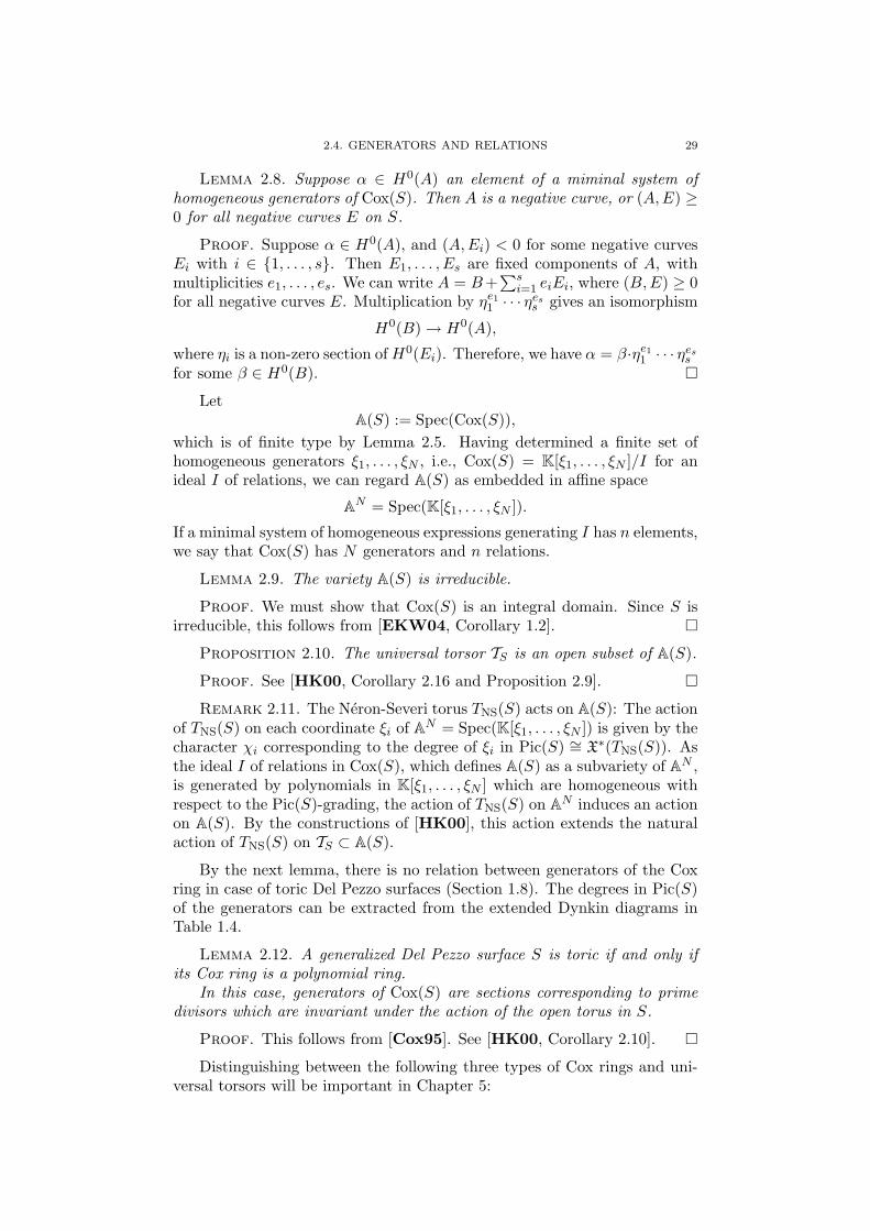
Lemma 2.8. Suppose α ∈ H0(A) an element of a miminal system ofhomogeneous generators of Cox(S). Then A is a negative curve, or (A,E) ≥0 for all negative curves E on S.
Proof. Suppose α ∈ H0(A), and (A,Ei) < 0 for some negative curvesEi with i ∈ {1, . . . , s}. Then E1, . . . , Es are fixed components of A, withmultiplicities e1, . . . , es. We can write A = B+
∑si=1 eiEi, where (B,E) ≥ 0
for all negative curves E. Multiplication by ηe11 · · · ηes
s gives an isomorphism
H0(B) → H0(A),
where ηi is a non-zero section ofH0(Ei). Therefore, we have α = β·ηe11 · · · ηes
s
for some β ∈ H0(B). �
LetA(S) := Spec(Cox(S)),
which is of finite type by Lemma 2.5. Having determined a finite set ofhomogeneous generators ξ1, . . . , ξN , i.e., Cox(S) = K[ξ1, . . . , ξN ]/I for anideal I of relations, we can regard A(S) as embedded in affine space
AN = Spec(K[ξ1, . . . , ξN ]).
If a minimal system of homogeneous expressions generating I has n elements,we say that Cox(S) has N generators and n relations.
Lemma 2.9. The variety A(S) is irreducible.
Proof. We must show that Cox(S) is an integral domain. Since S isirreducible, this follows from [EKW04, Corollary 1.2]. �
Proposition 2.10. The universal torsor TS is an open subset of A(S).
Proof. See [HK00, Corollary 2.16 and Proposition 2.9]. �
Remark 2.11. The Neron-Severi torus TNS(S) acts on A(S): The actionof TNS(S) on each coordinate ξi of AN = Spec(K[ξ1, . . . , ξN ]) is given by thecharacter χi corresponding to the degree of ξi in Pic(S) ∼= X∗(TNS(S)). Asthe ideal I of relations in Cox(S), which defines A(S) as a subvariety of AN ,is generated by polynomials in K[ξ1, . . . , ξN ] which are homogeneous withrespect to the Pic(S)-grading, the action of TNS(S) on AN induces an actionon A(S). By the constructions of [HK00], this action extends the naturalaction of TNS(S) on TS ⊂ A(S).
By the next lemma, there is no relation between generators of the Coxring in case of toric Del Pezzo surfaces (Section 1.8). The degrees in Pic(S)of the generators can be extracted from the extended Dynkin diagrams inTable 1.4.
Lemma 2.12. A generalized Del Pezzo surface S is toric if and only ifits Cox ring is a polynomial ring.
In this case, generators of Cox(S) are sections corresponding to primedivisors which are invariant under the action of the open torus in S.
Proof. This follows from [Cox95]. See [HK00, Corollary 2.10]. �
Distinguishing between the following three types of Cox rings and uni-versal torsors will be important in Chapter 5:

30 2. UNIVERSAL TORSORS AND COX RINGS
Lemma 2.13. Let S be a generalized Del Pezzo surface of degree 9 − r,with universal torsor TS. Let N be the minimal number of generators ofCox(S) ∼= K[ξ1, . . . , ξN ]/I, where I is the ideal of relations between thesegenerators.
• It is an open subset of affine space if and only if N = r + 3, and Iis trivial.
• It is an open subset of a hypersurface if and only if N = r+ 4, andI has one generator.
• It has codimension ≥ 2 in AN if and only if N ≥ r + 5, and I hasat least two independent generators.
Proof. For the dimension of the universal torsor, we have
dim(TS) = dim(S) + dim(TNS(S)) = r + 3.
As the universal torsor is an open subset of A(S) by Proposition 2.10, Cox(S)is a free polynomial ring with r+3 generators, or it has r+4 generators whoseideal of relations is generated by one equation, or at least r + 5 generatorsand at least two independent relations. �
CHAPTER 3
Cox rings of smooth Del Pezzo surfaces
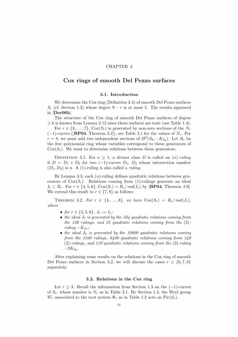
3.1. Introduction
We determine the Cox ring (Definition 2.4) of smooth Del Pezzo surfacesSr (cf. Section 1.3) whose degree 9 − r is at most 5. The results appearedin [Der06b].
The structure of the Cox ring of smooth Del Pezzo surfaces of degree≥ 6 is known from Lemma 2.12 since these surfaces are toric (see Table 1.4).
For r ∈ {3, . . . , 7}, Cox(Sr) is generated by non-zero sections of the Nr
(−1)-curves ([BP04, Theorem 3.2]), see Table 3.1 for the values of Nr. Forr = 8, we must add two independent sections of H0(S8,−KS8). Let Rr bethe free polynomial ring whose variables correspond to these generators ofCox(Sr). We want to determine relations between these generators.
Definition 3.1. For n ≥ 1, a divisor class D is called an (n)-rulingif D = D1 + D2 for two (−1)-curves D1, D2 whose intersection number(D1, D2) is n. A (1)-ruling is also called a ruling .
By Lemma 3.3, each (n)-ruling defines quadratic relations between gen-erators of Cox(Sr). Relations coming from (1)-rulings generate an idealIr ⊂ Rr. For r ∈ {4, 5, 6}, Cox(Sr) = Rr/ rad(Ir) by [BP04, Theorem 4.9].We extend this result to r ∈ {7, 8} as follows:
Theorem 3.2. For r ∈ {4, . . . , 8}, we have Cox(Sr) = Rr/ rad(Jr),where
• for r ∈ {4, 5, 6}, Jr := Ir;• the ideal J7 is generated by the 504 quadratic relations coming from
the 126 rulings, and 25 quadratic relations coming from the (2)-ruling −KS7;
• the ideal J8 is generated by the 10800 quadratic relations comingfrom the 2160 rulings, 6480 quadratic relations coming from 240(2)-rulings, and 119 quadratic relations coming from the (3)-ruling−2KS8.
After explaining some results on the relations in the Cox ring of smoothDel Pezzo surfaces in Section 3.2, we will discuss the cases r ∈ {6, 7, 8}separately.
3.2. Relations in the Cox ring
Let r ≥ 3. Recall the information from Section 1.3 on the (−1)-curvesof Sr, whose number is Nr as in Table 3.1. By Section 1.4, the Weyl groupWr associated to the root system Φr as in Table 1.2 acts on Pic(Sr).
31

32 3. COX RINGS OF SMOOTH DEL PEZZO SURFACES
For r ≤ 6, the relations in the Cox ring are induced by rulings, andthese relations also play an important role for r ∈ {7, 8}. More precisely,by the discussion following [BP04, Remark 4.7], each ruling is representedin r − 1 different ways as the sum of two (−1)-curves, giving r − 3 linearlyindependent quadratic relations in Cox(Sr). Therefore, if each of the Nr
(−1)-curves intersects nr (−1)-curves with intersection number 1, we haveN ′
r = (Nr · nr)/2 pairs, the number of rulings is N ′′r = N ′
r/(r − 1), andthe number of quadratic relations coming from rulings is N ′′
r · (r − 3) (seeTable 3.1).
r 3 4 5 6 7 8Nr 6 10 16 27 56 240nr 2 3 5 10 27 126N ′′
r 3 5 10 27 126 2160relations 0 5 20 81 504 10800
Table 3.1. The number of relations coming from rulings.
Now we describe how to obtain explicit equations for Cox(Sr) and howto prove Theorem 3.2. We isolate the steps that must be carried out for eachof the degrees 3, 2, and 1 and complete the proofs in the following sections.
Choice of coordinates. Choose coordinates for p1, . . . , pr ∈ P2. ByRemark 1.17, we may assume that the first four points are
(3.1) p1 = (1 : 0 : 0), p2 = (0 : 1 : 0), p3 = (0 : 0 : 1), p4 = (1 : 1 : 1),
and we can write pj = (1 : αj : βj) for j ∈ {5, . . . , r}.Curves in P2. As explained in the introduction, Cox(Sr) is generated
by sections of the (−1)-curves for r ≤ 7. For a (−1)-curve D, we denote thecorresponding section by ξ(D), and for a generating section ξ, letD(ξ) be thecorresponding divisor. For r = 8, we need two further generators: linearlyindependent sections κ1, κ2 of −KS8 . Let K1 := D(κ1), K2 := D(κ2) be thecorresponding divisors in the divisor class −KS8 .
LetDr be the set of divisors corresponding to sections generating Cox(Sr)(including K1,K2 if r = 8).
We need an explicit description of the image of each generator D ofCox(Sr) under the projection π : Sr → P2. According to Lemma 1.14, π(D)can be a curve, determined by a form fD of degree d ∈ {1, . . . , 6}, or a point(if D = Ei). If π(D) is a point, the convention to choose fD as a non-zeroconstant will be useful later.
For r = 8, we have the following situation: The image of Ki is a cubicthrough the eight points p1, . . . , p8. The choice of two linearly independentsections κ1, κ2 corresponds to the choice of two independent cubic formsfK1 , fK2 vanishing in the eight points. Every cubic through these points hasthe form a1fK1+a2fK2 where (a1, a2) 6= (0, 0), and the cubic does not changeif we replace (a1, a2) be a non-zero multiple. This gives a one-dimensionalprojective space of cubics through the eight points.

3.2. RELATIONS IN THE COX RING 33
LetX1, . . . , Xn be the monomials of degree d in three variables x0, x1, x2.For D ∈ Dr, we can write
fD =n∑
i=1
ai ·Xi
for suitable coefficients ai, which we can calculate in the following way: Ifpj lies on π(D), this gives a linear condition on the coefficients ai by substi-tuting the coordinates of pj for x0, x1, x2. If pj is a double point of π(D), allpartial derivatives of fD must vanish at this point, giving three more linearconditions. If pj is a triple point, we get six more linear conditions from thesecond derivatives. With p1, . . . , pr in general position, we check that theseconditions determine fD uniquely up to a non-zero constant.
Relations corresponding to (n)-rulings. Suppose that an (n)-rulingD can be written as Dj + D′
j for k different pairs Dj , D′j ∈ Dr where j ∈
{1, . . . , k}. Then the products
fD1 · fD′1, . . . , fDk
· fD′k
are k homogeneous forms of the same degree d, and they span a vector spaceof dimension n + 1 in the space of homogeneous polynomials of degree d.Consequently, there are k − (n + 1) independent relations between them,which we write as
k∑j=1
aj,i · fDj · fD′j
= 0 for i ∈ {1, . . . , k − (n+ 1)}.
for suitable constants aj,i. They give an explicit description of the quadraticrelations coming from D:
Lemma 3.3. In this situation, the (n)-ruling D gives the following k −(n+ 1) quadratic relations in Cox(Sr):
FD,i :=k∑
j=1
aj,i · ξ(Dj) · ξ(D′j) = 0 for i ∈ {1, . . . , k − (n+ 1)}.
We will describe the (n)-rulings in more detail in the subsequent sections.Let Jr be the ideal in Rr which is generated by the (n)-rulings (where
n = 1 for r ≤ 6, n ∈ {1, 2} for r = 7, and n ∈ {1, 2, 3} for r = 8).The proof of Theorem 3.2. For r ∈ {4, 5, 6}, this is [BP04, Theo-
rem 4.9]. For r ∈ {7, 8}, we use a refinement of its proof.Let Zr = Spec(Rr/ rad(Jr)) ⊂ Spec(Rr). We want to prove that Zr
equals A(Sr) ⊂ Spec(Rr), where A(Sr) := Spec(Cox(Sr)). Obviously, 0 ∈Spec(Rr) is contained in both Zr and A(Sr). Its complement Spec(Rr)\{0}is covered by the open sets
UD := {ξ(D) 6= 0}, where D ∈ Dr.
In the case r = 8, we will show that it suffices to consider the sets UD forD ∈ D8 \ {K1,K2}.
We want to show
Zr ∩ UD∼= Zr−1 × (A1 \ {0}).

34 3. COX RINGS OF SMOOTH DEL PEZZO SURFACES
Note that we can identify the (−1)-curves Dr−1 of Sr−1 with the subset D′r
of Dr containing the (−1)-curves which do not intersect D. We define
ψ : Zr ∩ UD → Zr−1 × (A1 \ {0})(ξ(D′) | D′ ∈ Dr) 7→ ((ξ(D′) | D′ ∈ Dr−1), ξ(D)) .
For r ∈ {7, 8}, we will prove:
Lemma 3.4. Every ξ(D′′) for D′′ ∈ Dr intersecting D is determined by
ξ(D) and {ξ(D′) | D′ ∈ Dr with (D′, D) = 0},provided that ξ(D) 6= 0 and using the relations generating Jr.
By the proof of [BP04, Proposition 4.4],
A(Sr) ∩ UD∼= A(Sr−1)× (A1 \ {0}).
By induction, Zr−1 = A(Sr−1). Therefore, Zr ∩ UD = A(Sr) ∩ UD forevery (−1)-curve D, which implies Zr = A(Sr), completing the proof ofTheorem 3.2 once Lemma 3.4 is proved.
3.3. Degree 3
We consider the case r = 6, i.e., smooth cubic surfaces. By Lemma 1.14,the set D6 of (−1)-curves on S6 consists of the following 27 divisors:
• exceptional divisors E1, . . . , E6, preimages of p1, . . . , p6 ∈ P2,• strict transforms mi,j = H − Ei − Ej of the 15 lines m′
i,j throughthe points pi, pj (i 6= j ∈ {1, . . . , 6}), and
• strict transforms Qk = 2H − (E1 + · · ·+E6) +Ek of the six conicsQ′
k through all of the blown-up points except pk.With respect to the anticanonical embedding S6 ↪→ P3, the (−1)-curves arethe 27 lines (Remark 1.26).
Together with information from Section 3.2, it is straightforward to de-rive:
Lemma 3.5. The extended Dynkin diagram of (−1)-curves has the fol-lowing structure:
(1) It has 27 vertices corresponding to the 27 lines Ei,mi,j , Qi. Eachof them has self-intersection number −1.
(2) Every line intersects exactly 10 other lines: Ei intersects mi,j andQj (for j 6= i); mi,j intersects Ei, Ej , Qi, Qj and mk,l (for {i, j} ∩{k, l} = ∅); Qi intersects mi,j and Ej (for j 6= i). Correspondingly,there are 135 edges in the Dynkin diagram.
(3) There are 45 triangles, i.e., triples of lines which intersect pairwise:30 triples Ei,mi,j , Qj and 15 triples of the form mi1,j1 ,mi2,j2 ,mi3,j3
where {i1, j1, i2, j2, i3, j3} = {1, . . . , 6}. This corresponds to 45 tri-angles in the Dynkin diagram, where each edge is contained in ex-actly one of the triangles, and each vertex belongs to exactly fivetriangles.
Lemma 3.6. The 27 rulings of S6 are given by −KS6 −D for D ∈ D6.Two (−1)-curves D′, D′′ fulfill D′+D′′ = −KS6−D if and only if D,D′, D′′
form a triangle in the sense of Lemma 3.5(3). There are five such pairs forany given D.

3.3. DEGREE 3 35
Proof. We can check directly that D +D′ +D′′ = −KS6 if D,D′, D′′
form a triangle. Therefore, −KS6 − D is a ruling. As any D is containedin exactly five triangles, this ruling can be expressed in five correspondingways as D′ +D′′.
On the other hand, by Table 3.1, the total number of rulings is 27, andeach ruling can be expressed in exactly five ways as the sum of two (−1)-curves. �
Let D be one of the 27 lines of S6, and consider the projection ψD :S6 → P1 from D. Then
ψ∗D(OP2(1)) = −KS6 −D =
H − Ei, D = Qi,
2H − (E1 + · · ·+ E6) + Ei + Ej , D = mi,j ,
3H − (E1 + · · ·+ E6)− Ei, D = Ei.
These are exactly the rulings.A generating set of Cox(S6) is given by section ηi, µi,j , λi corresponding
to the 27 lines Ei,mi,j , Qi, respectively. We order them in the following way:
η1, . . . , η6, µ1,2, . . . , µ1,6, µ2,3, . . . , µ2,6, µ3,4, . . . , µ5,6, λ1, . . . , λ6.
LetR6 := K[ηi, µi,j , λi].
The quadratic monomials in H0(S6,−KS6−D) corresponding to the fiveways to express −KS6 −D as the sum of the (−1)-curves are
• µi,jηj if D = Qi
• ηiλj , ηjλi, µk1,k2µk3,k4 if D = µi,j ({i, j, k1, . . . , k4} = {1, . . . , 6})• µi,jλj if D = Ei
In order to calculate the 81 relations in J6 explicitly as described inLemma 3.3, we use the coordinates of (3.1) for p1, . . . , p4, and
p5 = (1 : a : b), p6 = (1 : c : d).
We write
E := (b− 1)(c− 1)− (a− 1)(d− 1) and F := bc− ad
for simplicity. The three relations corresponding to a line D are denoted byF−KS6
−D,1, F−KS6−D,2, F−KS6
−D,3.
F−KS6−Q1,1 = −η2µ1,2 − η3µ1,3 + η4µ1,4
F−KS6−Q1,2 = −aη2µ1,2 − bη3µ1,3 + η5µ1,5
F−KS6−Q1,2 = −cη2µ1,2 − dη3µ1,3 + η6µ1,6
F−KS6−Q2,1 = η1µ1,2 − η3µ2,3 + η4µ2,4
F−KS6−Q2,2 = η1µ1,2 − bη3µ2,3 + η5µ2,5
F−KS6−Q2,3 = η1µ1,2 − dη3µ2,3 + η6µ2,6
F−KS6−Q3,1 = η1µ1,3 + η2µ2,3 + η4µ3,4
F−KS6−Q3,2 = η1µ1,3 + aη2µ2,3 + η5µ3,5
F−KS6−Q3,3 = η1µ1,3 + cη2µ2,3 + η6µ3,6

36 3. COX RINGS OF SMOOTH DEL PEZZO SURFACES
F−KS6−Q4,1 = η1µ1,4 + η2µ2,4 + η3µ3,4
F−KS6−Q4,2 = (1− b)η1µ1,4 + (a− b)η2µ2,4 + η5µ4,5
F−KS6−Q4,3 = (1− d)η1µ1,4 + (c− d)η2µ2,4 + η6µ4,6
F−KS6−Q5,1 = 1/bη1µ1,5 + a/bη2µ2,5 + η3µ3,5
F−KS6−Q5,2 = (1− b)/bη1µ1,5 + (a− b)/bη2µ2,5 + η4µ4,5
F−KS6−Q5,3 = (b− d)/bη1µ1,5 + F/bη2µ2,5 + η6µ5,6
F−KS6−Q6,1 = 1/dη1µ1,6 + c/dη2µ2,6 + η3µ3,6
F−KS6−Q6,2 = (1− d)/dη1µ1,6 + (c− d)/dη2µ2,6 + η4µ4,6
F−KS6−Q6,3 = (b− d)/dη1µ1,6 + F/dη2µ2,6 + η5µ5,6
F−KS6−m1,2,1 = µ4,5µ3,6 − µ3,5µ4,6 + µ3,4µ5,6
F−KS6−m1,2,2 = (b− d)µ3,5µ4,6 + (d− 1)µ3,4µ5,6 + η2λ1
F−KS6−m1,2,3 = Fµ3,5µ4,6 + a(d− c)µ3,4µ5,6 + η1λ2
F−KS6−m1,3,1 = µ4,5µ2,6 − µ2,5µ4,6 + µ2,4µ5,6
F−KS6−m1,3,2 = (c− a)µ2,5µ4,6 + (1− c)µ2,4µ5,6 + η3λ1
F−KS6−m1,3,3 = −Fµ2,5µ4,6 + b(c− d)µ2,4µ5,6 + η1λ3
F−KS6−m2,3,1 = µ4,5µ1,6 − µ1,5µ4,6 + µ1,4µ5,6
F−KS6−m2,3,2 = (a− c)µ1,5µ4,6 + a(c− 1)µ1,4µ5,6 + η3λ2
F−KS6−m2,3,3 = (b− d)µ1,5µ4,6 + b(d− 1)µ1,4µ5,6 + η2λ3
F−KS6−m1,4,1 = µ3,5µ2,6 − µ2,5µ3,6 + µ2,3µ5,6
F−KS6−m1,4,2 = −Eµ2,5µ3,6 + (b− 1)(c− 1)µ2,3µ5,6 + η4λ1
F−KS6−m1,4,3 = −Fµ2,5µ3,6 + bcµ2,3µ5,6 + η1λ4
F−KS6−m2,4,1 = µ3,5µ1,6 − µ1,5µ3,6 + µ1,3µ5,6
F−KS6−m2,4,2 = Eµ1,5µ3,6 + (a− b)(c− 1)µ1,3µ5,6 + η4λ2
F−KS6−m2,4,3 = (b− d)µ1,5µ3,6 − bµ1,3µ5,6 + η2λ4
F−KS6−m3,4,1 = µ2,5µ1,6 − µ1,5µ2,6 + µ1,2µ5,6
F−KS6−m3,4,2 = −Eµ1,5µ2,6 + (a− b)(1− d)µ1,2µ5,6 + η4λ3
F−KS6−m3,4,3 = (c− a)µ1,5µ2,6 + aµ1,2µ5,6 + η3λ4

3.3. DEGREE 3 37
F−KS6−m1,5,1 = µ3,4µ2,6 − µ2,4µ3,6 + µ2,3µ4,6
F−KS6−m1,5,2 = −Eµ2,4µ3,6 + (a− c)(1− b)µ2,3µ4,6 + η5λ1
F−KS6−m1,5,3 = (d− c)µ2,4µ3,6 + cµ2,3µ4,6 + η1λ5
F−KS6−m2,5,1 = µ3,4µ1,6 − µ1,4µ3,6 + µ1,3µ4,6
F−KS6−m2,5,2 = aEµ1,4µ3,6 + (a− b)(c− a)µ1,3µ4,6 + η5λ2
F−KS6−m2,5,3 = (1− d)µ1,4µ3,6 − µ1,3µ4,6 + η2λ5
F−KS6−m3,5,1 = µ2,4µ1,6 − µ1,4µ2,6 + µ1,2µ4,6
F−KS6−m3,5,2 = −bEµ1,4µ2,6 + (a− b)(b− d)µ1,2µ4,6 + η5λ3
F−KS6−m3,5,3 = (c− 1)µ1,4µ2,6 + µ1,2µ4,6 + η3λ5
F−KS6−m4,5,1 = µ2,3µ1,6 − µ1,3µ2,6 + µ1,2µ3,6
F−KS6−m4,5,2 = b(c− a)µ1,3µ2,6 + a(b− d)µ1,2µ3,6 + η5λ4
F−KS6−m4,5,3 = (c− 1)µ1,3µ2,6 + (1− d)µ1,2µ3,6 + η4λ5
F−KS6−m1,6,1 = µ3,4µ2,5 − µ2,4µ3,5 + µ2,3µ4,5
F−KS6−m1,6,2 = −Eµ2,4µ3,5 + (a− c)(1− d)µ2,3µ4,5 + η6λ1
F−KS6−m1,6,3 = (b− a)µ2,4µ3,5 + aµ2,3µ4,5 + η1λ6
F−KS6−m2,6,1 = µ3,4µ1,5 − µ1,4µ3,5 + µ1,3µ4,5
F−KS6−m2,6,2 = cEµ1,4µ3,5 + (a− c)(d− c)µ1,3µ4,5 + η6λ2
F−KS6−m2,6,3 = (1− b)µ1,4µ3,5 − µ1,3µ4,5 + η2λ6
F−KS6−m3,6,1 = µ2,4µ1,5 − µ1,4µ2,5 + µ1,2µ4,5
F−KS6−m3,6,2 = −dEµ1,4µ2,5 + (d− b)(d− c)µ1,2µ4,5 + η6λ3
F−KS6−m3,6,3 = (a− 1)µ1,4µ2,5 + µ1,2µ4,5 + η3λ6
F−KS6−m4,6,1 = µ2,3µ1,5 − µ1,3µ2,5 + µ1,2µ3,5
F−KS6−m4,6,2 = d(c− a)µ1,3µ2,5 + c(b− d)µ1,2µ3,5 + η6λ4
F−KS6−m4,6,3 = (a− 1)µ1,3µ2,5 + (1− b)µ1,2µ3,5 + η4λ6
F−KS6−m5,6,1 = µ2,3µ1,4 − µ1,3µ2,4 + µ1,2µ3,4
F−KS6−m5,6,2 = d(c− 1)µ1,3µ2,4 + c(1− d)µ1,2µ3,4 + η6λ5
F−KS6−m5,6,3 = b(a− 1)µ1,3µ2,4 + a(1− b)µ1,2µ3,4 + η5λ6
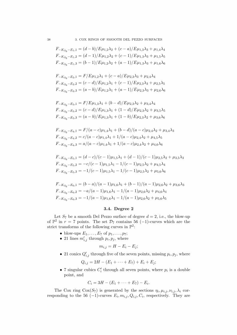
38 3. COX RINGS OF SMOOTH DEL PEZZO SURFACES
F−KS6−E1,1 = (d− b)/Eµ1,2λ2 + (c− a)/Eµ1,3λ3 + µ1,4λ4
F−KS6−E1,2 = (d− 1)/Eµ1,2λ2 + (c− 1)/Eµ1,3λ3 + µ1,5λ5
F−KS6−E1,3 = (b− 1)/Eµ1,2λ2 + (a− 1)/Eµ1,3λ3 + µ1,6λ6
F−KS6−E2,1 = F/Eµ1,2λ1 + (c− a)/Eµ2,3λ3 + µ2,4λ4
F−KS6−E2,2 = (c− d)/Eµ1,2λ1 + (c− 1)/Eµ2,3λ3 + µ2,5λ5
F−KS6−E2,3 = (a− b)/Eµ1,2λ1 + (a− 1)/Eµ2,3λ3 + µ2,6λ6
F−KS6−E3,1 = F/Eµ1,3λ1 + (b− d)/Eµ2,3λ2 + µ3,4λ4
F−KS6−E3,2 = (c− d)/Eµ1,3λ1 + (1− d)/Eµ2,3λ2 + µ3,5λ5
F−KS6−E3,3 = (a− b)/Eµ1,3λ1 + (1− b)/Eµ2,3λ2 + µ3,6λ6
F−KS6−E4,1 = F/(a− c)µ1,4λ1 + (b− d)/(a− c)µ2,4λ2 + µ3,4λ3
F−KS6−E4,2 = c/(a− c)µ1,4λ1 + 1/(a− c)µ2,4λ2 + µ4,5λ5
F−KS6−E4,3 = a/(a− c)µ1,4λ1 + 1/(a− c)µ2,4λ2 + µ4,6λ6
F−KS6−E5,1 = (d− c)/(c− 1)µ1,5λ1 + (d− 1)/(c− 1)µ2,5λ2 + µ3,5λ3
F−KS6−E5,2 = −c/(c− 1)µ1,5λ1 − 1/(c− 1)µ2,5λ2 + µ4,5λ4
F−KS6−E5,3 = −1/(c− 1)µ1,5λ1 − 1/(c− 1)µ2,5λ2 + µ5,6λ6
F−KS6−E6,1 = (b− a)/(a− 1)µ1,6λ1 + (b− 1)/(a− 1)µ2,6λ2 + µ3,6λ3
F−KS6−E6,2 = −a/(a− 1)µ1,6λ1 − 1/(a− 1)µ2,6λ2 + µ4,6λ4
F−KS6−E6,3 = −1/(a− 1)µ1,6λ1 − 1/(a− 1)µ2,6λ2 + µ5,6λ5
3.4. Degree 2
Let S7 be a smooth Del Pezzo surface of degree d = 2, i.e., the blow-upof P2 in r = 7 points. The set D7 contains 56 (−1)-curves which are thestrict transforms of the following curves in P2:
• blow-ups E1, . . . , E7 of p1, . . . , p7;• 21 lines m′
i,j through pi, pj , where
mi,j = H − Ei − Ej ;
• 21 conics Q′i,j through five of the seven points, missing pi, pj , where
Qi,j = 2H − (E1 + · · ·+ E7) + Ei + Ej ;
• 7 singular cubics C ′i through all seven points, where pi is a double
point, and
Ci = 3H − (E1 + · · ·+ E7)− Ei.
The Cox ring Cox(S7) is generated by the sections ηi, µi,j , νi,j , λi cor-responding to the 56 (−1)-curves Ei,mi,j , Qi,j , Ci, respectively. They are

3.4. DEGREE 2 39
ordered as
η1, . . . , η7, µ1,2, . . . , µ1,7, µ2,3, . . . , µ6,7, ν1,2, . . . , ν1,7, ν2,3, . . . , ν6,7, λ1, . . . , λ7.
LetR7 := K[ηi, µi,j , νi,j , λi]
be the polynomial ring in 56 generators.Consider the ideal I7 ⊂ R7 generated by the quadratic relations corre-
sponding to rulings. In view of Lemma 3.3, we need to know the six differentways to write each of the 126 rulings as a sum of two (−1)-curves in orderto describe I7 explicitly. Here, we do not write the resulting 504 relationsdown because of the length of this list.
Lemma 3.7. Each of the 126 rulings can be written in six ways as a sumof two (−1)-curves:
(1) For the seven rulings H − Ei:
{Ej +mi,j | j 6= i}.(2) For the 35 rulings 2H − (E1 + · · ·+ E7) + Ei + Ej + Ek:
{Ei +Qj,k, Ej +Qi,k, Ek +Qi,j ,ml1,l2 +ml3,l4 | {i, j, k, l1, l2, l3, l4} = {1, . . . , 7}}
(3) For the 42 rulings 3H − (E1 + · · ·+ E7) + Ei − Ej:
{Ei + Cj , Qi,k +mj,k | k 6= i, j}.(4) For the 35 rulings 4H − (E1 + · · ·+ E7)− Ei − Ej − Ek:
{Ci +mj,k, Cj +mi,k, Ck +mi,j , Ql1,l2 +Ql3,l4 | {i, j, k, l1, l2, l3, l4} = {1, . . . , 7}}
(5) For the seven rulings 5H − 2(E1 + · · ·+ E7) + Ei:
{Cj +Qi,j | j 6= i}.
However, we have more quadratic relations in Cox(S7): Note that thepoint q, with η1 = λ1 = 1 and other coordinates zero, satisfies the 504relations. Indeed, (E1, C1) = 2, but all quadratic monomials which occur inthe relations correspond to pairs of divisors whose intersection number is 1.Hence, all these monomials and all the relations vanish in q. On the otherhand, we check that the 504× 56 Jacobian matrix has rank 54 in this point,which means that q is contained in a component of the variety defined byI7 which has dimension 2. As A(S7) is irreducible of dimension 10, we mustfind other relations to exclude such components.
As E1 + C1 = −KS7 , we look for more relations in degree −KS7 ofCox(S7): We check that in this degree, we have exactly 28 monomials:
{ηiλi | 1 ≤ i ≤ 7} ∪ {µj,kνj,k | 1 ≤ j < k ≤ 7},corresponding to −KS7 = Ei +Ci = mj,k +Qj,k. As dimH0(S7,−KS7) = 3,and as none of the relations coming from rulings induces a relation in thisdegree, we obtain 25 independent relations. Note that −KS7 is the unique(2)-ruling of S7.
We can calculate the relations explicitly as they correspond to the rela-tions between the polynomials fEi · fCi and fmi,j · fQi,j , which are homoge-neous of degree 3, as described in Lemma 3.3.
Let J7 be the ideal generated by these 529 relations.

40 3. COX RINGS OF SMOOTH DEL PEZZO SURFACES
Proof of Lemma 3.4. In order to show that Cox(S7) is described byrad(J7), we must prove Lemma 3.4 in the case r = 7.
For any D ∈ D7, consider a coordinate ξ(D′) where (D,D′) = 1. This isdetermined by the ruling D + D′. Indeed, this ruling induces a relation ofthe form
ξ(D)ξ(D′) =∑
aiξ(Di)ξ(D′i),
where Di +D′i = D +D′. Therefore,
(D,Di +D′i) = (D,D +D′) = (D,D) + (D,D′) = −1 + 1 = 0,
which implies (D,Di) = (D,D′i) = 0 since the only (−1)-curve intersecting
D negatively is D itself. Since ξ(D) 6= 0, the only unknown variable ξ(D′)is determined by this relation.
Furthermore, there is exactly one coordinate ξ(D′′) where (D,D′′) = 2.The unique (2)-ruling D +D′′ = −KS7 induces a relation of the form
ξ(D)ξ(D′′) =∑
aiξ(Di)ξ(D′i),
where ξ(D′′) is the only unknown variable.
3.5. Degree 1
In this section, we consider blow-ups of P2 in r = 8 points in generalposition, i.e., smooth Del Pezzo surfaces S8 of degree 1.
The set D8 contains the strict transforms of the following 242 curves:• Blow-ups E1, . . . , E8 of p1, . . . , p8;• 28 lines m′
i,j through pi, pj :
mi,j = H − Ei − Ej ;
• 56 conics Q′i,j,k through 5 points, missing pi, pj , pk:
Qi,j,k = 2H − (E1 + · · ·+ E8) + Ei + Ej + Ek;
• 56 cubics C ′i,j through 7 points missing pj , where pi is a double
point:
Ci,j = 3H − (E1 + · · ·+ E8)− Ei + Ej ;
• 56 quartics V ′i,j,k through all points, where pi, pj , pk are double
points:
Vi,j,k = 4H − (E1 + · · ·+ E8)− (Ei + Ej + Ek);
• 28 quintics F ′i,j through all points, where pi, pj are simple points
and the other six are double points:
Fi,j = 5H − 2(E1 + · · ·+ E8) + Ei + Ej ;
• 8 sextics T ′i , where pi a triple point and the other seven points aredouble points:
Ti = 6H − 2(E1 + · · ·+ E8)− Ei;
• two independent cubics K ′1,K
′2 through the eight points:
[K1] = [K2] = −KS8 = 3− (E1 + · · ·+ E8).
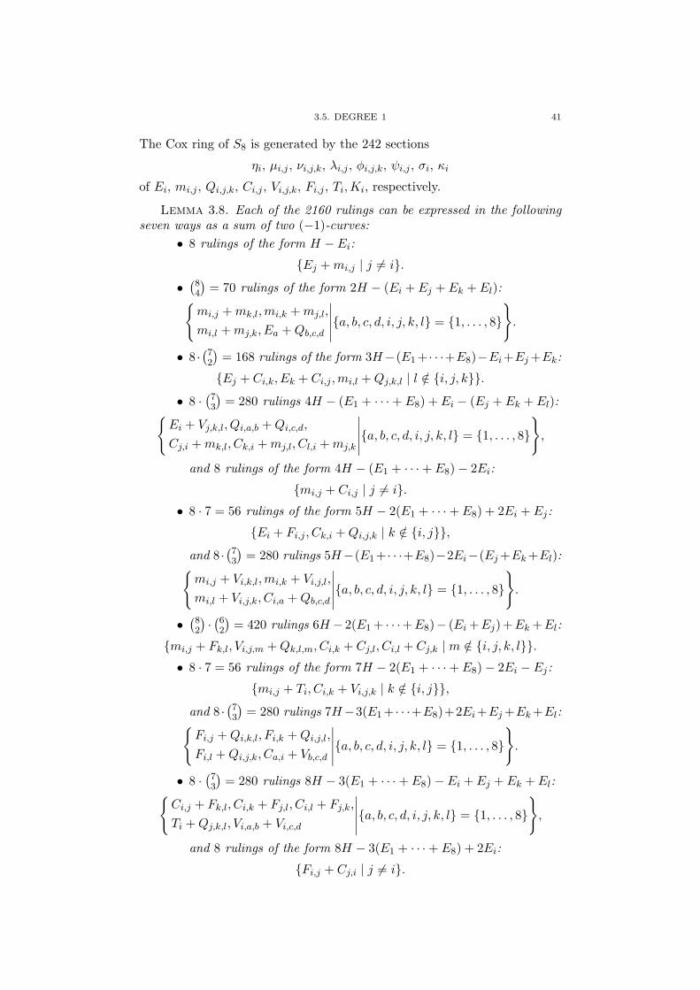
3.5. DEGREE 1 41
The Cox ring of S8 is generated by the 242 sections
ηi, µi,j , νi,j,k, λi,j , φi,j,k, ψi,j , σi, κi
of Ei, mi,j , Qi,j,k, Ci,j , Vi,j,k, Fi,j , Ti,Ki, respectively.
Lemma 3.8. Each of the 2160 rulings can be expressed in the followingseven ways as a sum of two (−1)-curves:
• 8 rulings of the form H − Ei:
{Ej +mi,j | j 6= i}.
•(84
)= 70 rulings of the form 2H − (Ei + Ej + Ek + El):{
mi,j +mk,l,mi,k +mj,l,
mi,l +mj,k, Ea +Qb,c,d
∣∣∣∣∣{a, b, c, d, i, j, k, l} = {1, . . . , 8}
}.
• 8 ·(72
)= 168 rulings of the form 3H−(E1+ · · ·+E8)−Ei +Ej +Ek:
{Ej + Ci,k, Ek + Ci,j ,mi,l +Qj,k,l | l /∈ {i, j, k}}.
• 8 ·(73
)= 280 rulings 4H − (E1 + · · ·+ E8) + Ei − (Ej + Ek + El):{
Ei + Vj,k,l, Qi,a,b +Qi,c,d,
Cj,i +mk,l, Ck,i +mj,l, Cl,i +mj,k
∣∣∣∣∣{a, b, c, d, i, j, k, l} = {1, . . . , 8}
},
and 8 rulings of the form 4H − (E1 + · · ·+ E8)− 2Ei:
{mi,j + Ci,j | j 6= i}.• 8 · 7 = 56 rulings of the form 5H − 2(E1 + · · ·+ E8) + 2Ei + Ej:
{Ei + Fi,j , Ck,i +Qi,j,k | k /∈ {i, j}},
and 8 ·(73
)= 280 rulings 5H−(E1+ · · ·+E8)−2Ei−(Ej +Ek +El):{
mi,j + Vi,k,l,mi,k + Vi,j,l,
mi,l + Vi,j,k, Ci,a +Qb,c,d
∣∣∣∣∣{a, b, c, d, i, j, k, l} = {1, . . . , 8}
}.
•(82
)·(62
)= 420 rulings 6H − 2(E1 + · · ·+E8)− (Ei +Ej)+Ek +El:
{mi,j + Fk,l, Vi,j,m +Qk,l,m, Ci,k + Cj,l, Ci,l + Cj,k | m /∈ {i, j, k, l}}.• 8 · 7 = 56 rulings of the form 7H − 2(E1 + · · ·+ E8)− 2Ei − Ej:
{mi,j + Ti, Ci,k + Vi,j,k | k /∈ {i, j}},
and 8 ·(73
)= 280 rulings 7H−3(E1 + · · ·+E8)+2Ei +Ej +Ek +El:{
Fi,j +Qi,k,l, Fi,k +Qi,j,l,
Fi,l +Qi,j,k, Ca,i + Vb,c,d
∣∣∣∣∣{a, b, c, d, i, j, k, l} = {1, . . . , 8}
}.
• 8 ·(73
)= 280 rulings 8H − 3(E1 + · · ·+ E8)− Ei + Ej + Ek + El:{
Ci,j + Fk,l, Ci,k + Fj,l, Ci,l + Fj,k,
Ti +Qj,k,l, Vi,a,b + Vi,c,d
∣∣∣∣∣{a, b, c, d, i, j, k, l} = {1, . . . , 8}
},
and 8 rulings of the form 8H − 3(E1 + · · ·+ E8) + 2Ei:
{Fi,j + Cj,i | j 6= i}.

42 3. COX RINGS OF SMOOTH DEL PEZZO SURFACES
• 8·(72
)= 168 rulings of the form 9H−3(E1+· · ·+E8)+Ei−(Ej+Ek):
{Sj + Ck,i, Sk + Cj,i, Fi,l + Vj,k,l | l /∈ {i, j, k}}.
•(84
)= 70 rulings of the form 10H−4(E1+· · ·+E8)+Ei+Ej+Ek+El:
{Fi,j +Fk,l, Fi,k +Fj,l, Fi,l +Fj,k, Sa+Vb,c,d | {a, b, c, d, i, j, k, l} = {1, . . . , 8}}.• 8 rulings of the form 11H − 4(E1 + · · ·+ E8) + Ei:
{Sj + Fi,j | j 6= i}.There is no way to write a ruling as the sum of −KS8 and (−1)-curves.
Proof. Because of the Weyl group symmetry, we need to prove the laststatement only in one case, say H − E1. In this case, it is obvious.
By Table 3.1, there can be no other rulings, and each ruling can beexpressed in no further ways as the sum of two (−1)-curves. �
With this information, Lemma 3.3 allows us to determine the 10800relations coming from rulings explicitly.
We can find more quadratic relations in the degrees corresponding to(2)-rulings: Because of the Weyl group symmetry, it is enough to considerthe (2)-ruling D := E2 +C2,1. This can also be written as Ej +Cj,1 for anyj 6= 1 and as mi,j + Q1,i,j for any i, j 6= 1, giving 28 section in H0(S8, D).As D = −KS8 + E1, we get two further section η1κ1, η1κ2. As the previousquadratic relations do not induce relations in this degree of Cox(S8), andbecause we calculate dimH0(S8, D) = 3 for this nef degree, we obtain 27relations, which can be calculated explicitly as before.
Every (−1)-curve has intersection number 2 with exactly 56 other curves(e.g. (E1, D) = 2 if and only if D ∈ {C1,i, V1,i,j , Fi,j , Ti} for i, j 6= 1), so itoccurs in exactly 56 (2)-rulings. On the other hand, as every (2)-ruling canbe written in 28 ways as the sum of two (−1)-curves, the total number of(2)-rulings is 240·56
2·28 = 240. Therefore, we obtain another 6480 relations fromthe (2)-rulings. To determine them explicitly, we need the following moredetailed information:
Lemma 3.9. Each of the 240 (2)-rulings can be written as a sum of two(−1)-curves in the following 28 ways:
• 8 (2)-rulings of the form
−KS8 + Ei = 3H − (E1 + · · ·+ E8) + Ei :
{Ej + Cj,i,mj,k +Qi,j,k | j, k 6= i}.•(82
)= 28 (2)-rulings of the form
−KS8 +mi,j = 4H − (E1 + · · ·+ E8)− (Ei + Ej) :{Ek + Vi,j,k,mi,k + Cj,k,
mj,k + Ci,k, Qa,b,c +Qd,e,f
∣∣∣∣∣ k /∈ {i, j},{i, j, a, b, c, d, e, f} = {1, . . . , 8}
}.
•(83
)= 56 (2)-rulings of the form
−KS8 +Qi,j,k = 5H − 2(E1 + · · ·+ E8) + Ei + Ej + Ek :{Ei + Fj,k, Ej + Fi,k, Ek + Fi,j ,ma,b + Vc,d,e,
Qi,j,l + Cl,k, Qi,k,l + Cl,j , Qj,k,l + Cl,i
∣∣∣∣∣ {i, j, k, a, b, c, d, e}= {1, . . . , 8}, l /∈ {i, j, k}
}.
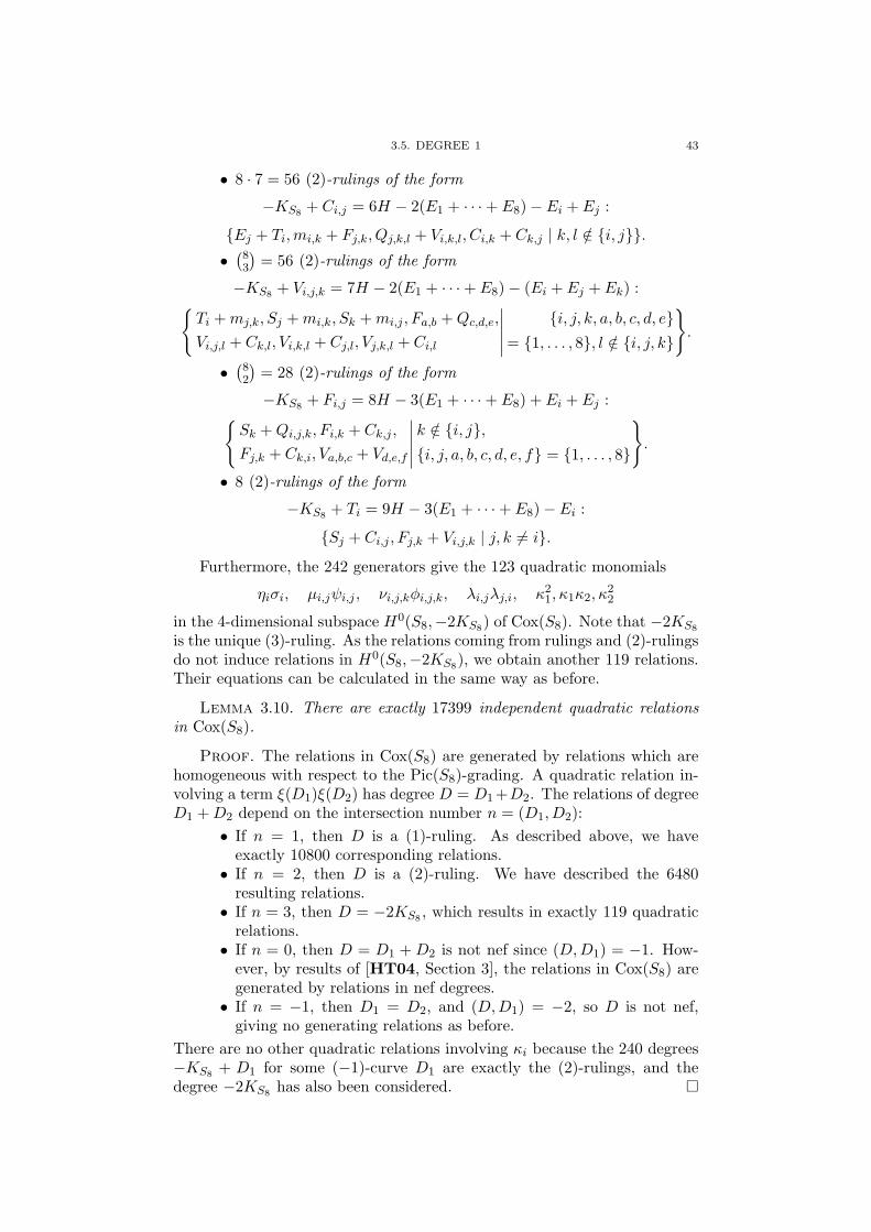
3.5. DEGREE 1 43
• 8 · 7 = 56 (2)-rulings of the form
−KS8 + Ci,j = 6H − 2(E1 + · · ·+ E8)− Ei + Ej :
{Ej + Ti,mi,k + Fj,k, Qj,k,l + Vi,k,l, Ci,k + Ck,j | k, l /∈ {i, j}}.•(83
)= 56 (2)-rulings of the form
−KS8 + Vi,j,k = 7H − 2(E1 + · · ·+ E8)− (Ei + Ej + Ek) :{Ti +mj,k, Sj +mi,k, Sk +mi,j , Fa,b +Qc,d,e,
Vi,j,l + Ck,l, Vi,k,l + Cj,l, Vj,k,l + Ci,l
∣∣∣∣∣ {i, j, k, a, b, c, d, e}= {1, . . . , 8}, l /∈ {i, j, k}
}.
•(82
)= 28 (2)-rulings of the form
−KS8 + Fi,j = 8H − 3(E1 + · · ·+ E8) + Ei + Ej :{Sk +Qi,j,k, Fi,k + Ck,j ,
Fj,k + Ck,i, Va,b,c + Vd,e,f
∣∣∣∣∣ k /∈ {i, j},{i, j, a, b, c, d, e, f} = {1, . . . , 8}
}.
• 8 (2)-rulings of the form
−KS8 + Ti = 9H − 3(E1 + · · ·+ E8)− Ei :
{Sj + Ci,j , Fj,k + Vi,j,k | j, k 6= i}.
Furthermore, the 242 generators give the 123 quadratic monomials
ηiσi, µi,jψi,j , νi,j,kφi,j,k, λi,jλj,i, κ21, κ1κ2, κ
22
in the 4-dimensional subspace H0(S8,−2KS8) of Cox(S8). Note that −2KS8
is the unique (3)-ruling. As the relations coming from rulings and (2)-rulingsdo not induce relations in H0(S8,−2KS8), we obtain another 119 relations.Their equations can be calculated in the same way as before.
Lemma 3.10. There are exactly 17399 independent quadratic relationsin Cox(S8).
Proof. The relations in Cox(S8) are generated by relations which arehomogeneous with respect to the Pic(S8)-grading. A quadratic relation in-volving a term ξ(D1)ξ(D2) has degree D = D1 +D2. The relations of degreeD1 +D2 depend on the intersection number n = (D1, D2):
• If n = 1, then D is a (1)-ruling. As described above, we haveexactly 10800 corresponding relations.
• If n = 2, then D is a (2)-ruling. We have described the 6480resulting relations.
• If n = 3, then D = −2KS8 , which results in exactly 119 quadraticrelations.
• If n = 0, then D = D1 +D2 is not nef since (D,D1) = −1. How-ever, by results of [HT04, Section 3], the relations in Cox(S8) aregenerated by relations in nef degrees.
• If n = −1, then D1 = D2, and (D,D1) = −2, so D is not nef,giving no generating relations as before.
There are no other quadratic relations involving κi because the 240 degrees−KS8 + D1 for some (−1)-curve D1 are exactly the (2)-rulings, and thedegree −2KS8 has also been considered. �

44 3. COX RINGS OF SMOOTH DEL PEZZO SURFACES
Let J8 be the ideal generated by these 17399 quadratic relations in
R8 = K[ηi, µi,j , νi,j,k, λi,j , φi,j,k, ψi,j , σi, κi].
Proof of Lemma 3.4. Let D ∈ D8 \ {K1,K2} be any (−1)-curve. Wecall a variable ξ(D′) for a (−1)-curve D′ ∈ D8 an (n)-variable if (D,D′) = n.
As for r = 7 in the previous section, we show that the rulings determinethe (1)-variables in terms of the (0)-variables and ξ(D) 6= 0.
For the two variables κi = ξ(Ki) corresponding to −KS8 , we use the (2)-ruling −KS8 +D: As (D,−KS8 +D) = 0, we have (D,Di) = (D,D′
i) = 0for any other possibility to write −KS8 +D as the sum of two (−1)-curvesDi, D
′i. Since (−KS8 + D,−KS8) = 2, by [BP04, Proposition 3.4], the
quadratic monomials ξ(Di)ξ(D′i) span H0(S8,−KS8 +D), so this (2)-ruling
induces relations of the form
κiξ(D) =∑
aiξ(Di)ξ(D′i).
Therefore, κ1, κ2 are determined by ξ(D) and the (0)-variables.Any (2)-coordinate ξ(D′) is determined by the (2)-ruling D + D′: As
(D,D+D′) = 1, we have (D,Di) = 0 and (D,D′i) = 1 for every other possi-
bility to write D+D′ as the sum of two (−1)-curves Di, D′i. Furthermore, if
D+D′ = −KS8 +D′′, then (D,D′′) = 0. Hence, the relations correspondingto this (2)-ruling determine ξ(D′) in terms of the (0)- and (1)-variables andκ1, κ2, ξ(D).
Finally, there is a unique (3)-coordinate D′, where D +D′ = −2KS8 isthe (3)-ruling. As all other variables are known at this point, the relationscorresponding to −2KS8 containing the term ξ(D)ξ(D′) determine ξ(D′).
Consider a point in UKj , i.e., with κj 6= 0. As above, by [BP04, Propo-sition 3.4], H0(S8,−2KS8) is spanned by the monomials ξ(Di)ξ(D′
i) for (3)-rulings Di, D
′i. Therefore, we have relations of the form
κ2j =
∑aiξ(Di)ξ(D′
i),
which shows that ξ(Di) 6= 0 for some i. This proves that Z8 \ {0} is coveredby the sets UD for D ∈ D8 \ {K1,K2}.

CHAPTER 4
Universal torsors and homogeneous spaces
4.1. Introduction
In this chapter, we continue our investigations of universal torsors oversmooth Del Pezzo surfaces over an algebraically closed field K of character-istic 0. The results first appeared in [Der06d].
The blow-up of P2 in r points in general position is a smooth Del Pezzosurface Sr of degree 9 − r; we will assume that r ∈ {3, . . . , 7}. The Picardgroup Pic(Sr) is a lattice with the non-degenerate intersection form (·, ·).As explained in Section 1.4, Pic(Sr) contains a canonical root system Φr,which carries the action of the associated Weyl group Wr, see Table 4.1.
r 3 4 5 6 7Φr A2 + A1 A4 D5 E6 E7
Nr 6 10 16 27 56
Table 4.1. The root systems associated to Del Pezzo surfaces.
It was a general expectation that the Weyl group symmetry on Pic(Sr)should be a reflection of a geometric link between Del Pezzo surfaces andalgebraic groups. Here we show that universal torsors of smooth Del Pezzosurfaces of degree 2 and 3 admit an embedding into a certain flag variety forthe corresponding algebraic group. The degree 5 case goes back to Salberger(talk at the Borel seminar Bern, June 1993) following Mumford [MS72],and independently Skorobogatov [Sko93]. The degree 4 case was treated inthe thesis of Popov [Pop01, Chapter 6]. The existence of such an embed-ding in general was conjectured by Batyrev in his lecture at the conferenceDiophantine geometry (Universitat Gottingen, June 2004). Skorobogatovannounced related work in progress (joint with Serganova) at the conferenceCohomological approaches to rational points (MSRI, March 2006).
By [BP04, Section 2], the simple roots of Φr−1 (with Φ2 = A2) canbe identified with a subset Ir of the simple roots of Φr whose complementconsists of exactly one simple root αr, with associated fundamental weight$r. The Weyl group Wr acts on the weight lattice of the linear algebraicgroup Gr associated to Φr. The fundamental representation %r of Gr withhighest weight $r has dimension Nr as listed in Table 4.1; the weights of %r
can be identified with classes of (−1)-curves E ⊂ Sr.Let Pr be the maximal parabolic subgroup corresponding to Ir, and let
Hr be the affine cone over Gr/Pr. It is well-known that Hr is given by qua-dratic equations in affine space ANr . For r = 6, the equations are all partial
45
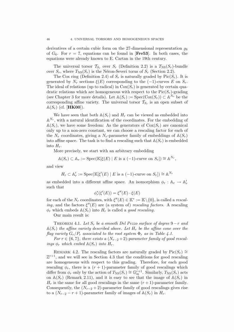
46 4. UNIVERSAL TORSORS AND HOMOGENEOUS SPACES
derivatives of a certain cubic form on the 27-dimensional representation %6
of G6. For r = 7, equations can be found in [Fre53]. In both cases, theequations were already known to E. Cartan in the 19th century.
The universal torsor TSr over Sr (Definition 2.2) is a TNS(Sr)-bundleover Sr, where TNS(Sr) is the Neron-Severi torus of Sr (Section 2.2).
The Cox ring (Definition 2.4) of Sr is naturally graded by Pic(Sr). It isgenerated by Nr sections ξ(E) corresponding to the (−1)-curves E on Sr.The ideal of relations (up to radical) in Cox(Sr) is generated by certain qua-dratic relations which are homogeneous with respect to the Pic(Sr)-grading(see Chapter 3 for more details). Let A(Sr) := Spec(Cox(Sr)) ⊂ ANr be thecorresponding affine variety. The universal torsor TSr is an open subset ofA(Sr) (cf. [HK00]).
We have seen that both A(Sr) and Hr can be viewed as embedded intoANr , with a natural identification of the coordinates. For the embedding ofA(Sr), we have some freedom: As the generators of Cox(Sr) are canonicalonly up to a non-zero constant, we can choose a rescaling factor for each ofthe Nr coordinates, giving a Nr-parameter family of embeddings of A(Sr)into affine space. The task is to find a rescaling such that A(Sr) is embeddedinto Hr.
More precisely, we start with an arbitrary embedding
A(Sr) ⊂ Ar := Spec(K[ξ(E) | E is a (−1)-curve on Sr]) ∼= ANr ,
and view
Hr ⊂ A′r := Spec(K[ξ′(E) | E is a (−1)-curve on Sr]) ∼= ANr
as embedded into a different affine space. An isomorphism φr : Ar → A′r
such thatφ∗r(ξ
′(E)) = ξ′′(E) · ξ(E)
for each of the Nr coordinates, with ξ′′(E) ∈ K∗ := K\{0}, is called a rescal-ing , and the factors ξ′′(E) are (a system of) rescaling factors. A rescalingφr which embeds A(Sr) into Hr is called a good rescaling .
Our main result is:
Theorem 4.1. Let Sr be a smooth Del Pezzo surface of degree 9− r andA(Sr) the affine variety described above. Let Hr be the affine cone over theflag variety Gr/Pr associated to the root system Φr as in Table 4.1.
For r ∈ {6, 7}, there exists a (Nr−2 +2)-parameter family of good rescal-ings φr which embed A(Sr) into Hr.
Remark 4.2. The rescaling factors are naturally graded by Pic(Sr) ∼=Zr+1, and we will see in Section 4.3 that the conditions for good rescalingare homogeneous with respect to this grading. Therefore, for each goodrescaling φr, there is a (r + 1)-parameter family of good rescalings whichdiffer from φr only by the action of TNS(Sr) ∼= Gr+1
m . Similarly, TNS(Sr) actson A(Sr) (Remark 2.11), and it is easy to see that the image of A(Sr) inHr is the same for all good rescalings in the same (r+ 1)-parameter family.Consequently, the (Nr−2 + 2)-parameter family of good rescalings gives riseto a (Nr−2 − r + 1)-parameter family of images of A(Sr) in Hr.

4.2. HOMOGENEOUS SPACES 47
For r = 5, we have Nr−2− r+1 = 2, and by [Pop01, Section 6.3], thereis a two-parameter family of images of A(S5) under good rescalings in H5.
In Section 4.2, we recall the classical equations for the homogeneousspaces Gr/Pr and give a simplified description on a certain Zariski opensubset; this will help to find good rescalings. In Section 4.3, we deriveconditions on the rescaling factors in terms of the description of Cox(Sr)and Gr/Pr. In Section 4.4 and Section 4.5, we determine good rescalings indegree 3 and 2, finishing the proof of Theorem 4.1.
4.2. Homogeneous spaces
In this section, we examine the equations defining the affine cone Hr ⊂A′
r over Gr/Pr for r ∈ {6, 7}. For the Nr coordinates ξ′(E) of A′r, we also
use the names η′i, µ′i,j , λ
′i, and furthermore ν ′i,j in the case r = 7.
These coordinates are in obvious correspondence to the coordinates ofAr, for which we use the names ηi, µi,j , λi (see Section 3.3), and furthermoreνi,j in the case r = 7 (see Section 3.4) as for the generators of Cox(Sr).
In particular, we show that Hr is a complete intersection on the opensubset Ur of A′
r where the coordinates η′1, . . . , η′r are non-zero.
We will see that Hr is defined by quadratic relations which are homo-geneous with respect to the Pic(Sr)-grading. For each (1)-ruling D, wehave exactly one relation pD of degree D, and furthermore in the caser = 7, we have eight relations p(1)
−KS7, . . . , p
(8)−KS7
where we use the con-
vention p−KS7:= p
(1)−KS7
. For any possibility to write D as the sum of two(−1)-curves E, E′, the relation pD has a term ξ′(E)ξ′(E′) with a non-zerocoefficient.
Definition 4.3. For a (−1)-curve E, let UE be the open subset of A′r
where ξ′(E) is non-zero. Let N (E)k be the set of (−1)-curves E′ with(E,E′) = k, and let Ξ′(E)k be the set of the corresponding ξ′(E′). LetN (E)>k and Ξ′(E)>k be defined similarly, but with the condition (E,E′) >k.
Let Ur ⊂ A′r be the intersection of UE1 , . . . , UEr .
Note that N (E)0 has exactly Nr−1 elements because we can identifyits elements with the (−1)-curves on Sr−1. Since the only (−1)-curve in-tersecting E negatively is E itself, the number of elements of N (E)>0 isNr −Nr−1 − 1.
Proposition 4.4. Let
Ψr : Hr ∩ Ur → Ur−1 × (A1 \ {0})be the projection to the coordinates ξ′(E) ∈ Ξ′(E1)0 and η′1. The map Ψr isan isomorphism. The dimension of Hr is Nr−1 + 1.
Proof. IfD = E1+E is a (1)-ruling, then (E1, D) = 0, and all variablesoccurring in pD besides η′1 and ξ′(E) are elements of Ξ′(E1)0. For η′1 6= 0,the relation pD expresses ξ′(E) in terms of η′1 and Ξ′(E1)0.
For a (2)-ruling D = E1 + E, we have (E1, D) = 1, so the relation pD
expresses ξ′(E) in terms of η′1 and monomials ξ′(E′i)ξ
′(E′′i ) where ξ(E′
i) ∈
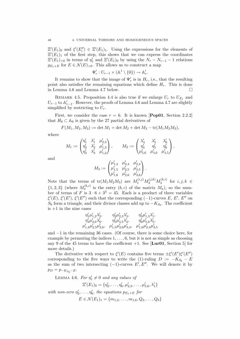
48 4. UNIVERSAL TORSORS AND HOMOGENEOUS SPACES
Ξ′(E1)0 and ξ′(E′′i ) ∈ Ξ′(E1)1. Using the expressions for the elements of
Ξ′(E1)1 of the first step, this shows that we can express the coordinatesΞ′(E1)>0 in terms of η′1 and Ξ′(E1)0 by using the Nr − Nr−1 − 1 relationsgE1+E for E ∈ N (E)>0. This allows us to construct a map
Ψ′r : Ur−1 × (A1 \ {0}) → A′
r.
It remains to show that the image of Ψ′r is in Hr, i.e., that the resulting
point also satisfies the remaining equations which define Hr. This is donein Lemma 4.6 and Lemma 4.7 below. �
Remark 4.5. Proposition 4.4 is also true if we enlarge Ur to UE1 andUr−1 to A′
r−1. However, the proofs of Lemma 4.6 and Lemma 4.7 are slightlysimplified by restricting to Ur.
First, we consider the case r = 6. It is known [Pop01, Section 2.2.2]that H6 ⊂ A6 is given by the 27 partial derivatives of
F (M1,M2,M3) := detM1 + detM2 + detM3 − tr(M1M2M3),
where
M1 :=
η′1 λ′1 µ′2,3
η′2 λ′2 µ′1,3
η′3 λ′3 µ′1,2
, M2 :=
λ′4 λ′5 λ′6η′4 η′5 η′6µ′5,6 µ′4,6 µ′4,5
,
and
M3 :=
µ′1,4 µ′2,4 µ′3,4
µ′1,5 µ′2,5 µ′3,5
µ′1,6 µ′2,6 µ′3,6
.
Note that the terms of tr(M1M2M3) are M(i,j)1 M
(j,k)2 M
(k,i)3 for i, j, k ∈
{1, 2, 3} (where M (b,c)a is the entry (b, c) of the matrix Ma), so the num-
ber of terms of F is 3 · 6 + 33 = 45. Each is a product of three variablesξ′(E), ξ′(E′), ξ′(E′′) such that the corresponding (−1)-curves E, E′, E′′ onS6 form a triangle, and their divisor classes add up to −KS6 . The coefficientis +1 in the nine cases
η′1µ′1,2λ
′2, η′2µ
′2,3λ
′3, η′3µ
′1,3λ
′1,
η′4µ′4,6λ
′6, η′5µ
′4,5λ
′4, η′6µ
′5,6λ
′5,
µ′1,4µ′2,5µ
′3,6, µ′1,5µ
′2,6µ
′3,4, µ′1,6µ
′2,4µ
′3,5
and −1 in the remaining 36 cases. (Of course, there is some choice here, forexample by permuting the indices 1, . . . , 6, but it is not as simple as choosingany 9 of the 45 terms to have the coefficient +1. See [Lur01, Section 5] formore details.)
The derivative with respect to ξ′(E) contains five terms ±ξ′(E′)ξ′(E′′)corresponding to the five ways to write the (1)-ruling D := −KS6 − Eas the sum of two intersecting (−1)-curves E′, E′′. We will denote it bypD = p−KS6
−E .
Lemma 4.6. For η′1 6= 0 and any values of
Ξ′(E1)0 = {η′2, . . . , η′6, µ′2,3, . . . , µ′5,6, λ
′1}
with non-zero η′2, . . . , η′6, the equations pE1+E for
E ∈ N (E1)1 = {m1,2, . . . ,m1,6, Q2, . . . , Q6}

4.2. HOMOGENEOUS SPACES 49
define a point of H6.
Proof. As TNS(S6) acts on H6 and {E1, . . . , E6} is a subset of a basisof Pic(S6), we may assume that η′1 = · · · = η′6 = 1. Then for i ∈ {2, . . . , 6},the equation pE1+m1,i allows us to express µ′1,i in terms of the remainingµ′i,j :
µ′1,2 = µ′2,3 + µ′2,4 + µ′2,5 + µ′2,6, µ′1,3 = µ′2,3 − µ′3,4 − µ′3,5 − µ′3,6,
µ′1,4 = −µ′2,4 − µ′3,4 + µ′4,5 − µ′4,6, µ′1,5 = −µ′2,5 − µ′3,5 − µ′4,5 + µ′5,6
µ′1,6 = −µ′2,6 − µ′3,6 + µ′4,6 − µ′5,6
Furthermore, for i ∈ {2, . . . , 6}, we can use pE1+Qi in order to express λ′i interms of λ′1 and µ′j,k:
λ′2 = µ′3,4µ′5,6 + µ′3,5µ
′4,6 + µ′3,6µ
′4,5 + λ′1
λ′3 = −µ′2,4µ′5,6 − µ′2,5µ
′4,6 − µ′2,6µ
′4,5 + λ′1
λ′4 = −µ′2,3µ′5,6 + µ′2,5µ
′3,6 − µ′2,6µ
′3,5 − λ′1
λ′5 = −µ′2,3µ′4,6 − µ′2,4µ
′3,6 + µ′2,6µ
′3,4 − λ′1
λ′6 = −µ′2,3µ′4,5 + µ′2,4µ
′3,5 − µ′2,5µ
′3,4 − λ′1
By substituting and expanding, we check that the remaining 17 relationsare fulfilled. Therefore, the resulting point lies in H6. �
Next, we obtain similar results in the case r = 7. The N7 = 56 coordi-nates ξ′(E) in A′
r are η′i, µ′j,k, ν
′j,k, λ
′i for i, j, k ∈ {1, . . . , 7} and j < k. The
equations for H7 are described in [Fre53] in terms of 56 coordinates xij , yij
(i < j ∈ {1, . . . , 8}). They correspond to our generators as follows:
η′i = xi8, µ′k,l = ykl, ν ′k,l = xkl, λ′i = yi8.
For the (1)-rulings D (see Lemma 3.7), the relations pD are uijkl andvij as below. In the first column of Table 4.2, we list a symbol D(n)
I as-signed to the (1)-ruling in the second column, and the third column givesthe corresponding relation.
symbol (1)-ruling D = D(n)I relation pD
D(1)i H − Ei v8
i
D(2)i,j,k 2H − (E1 + · · ·+ E7) + Ei + Ej + Ek uijk8
D(3)i,j 3H − (E1 + · · ·+ E7) + Ei − Ej vi
j
D(4)i,j,k,l 4H − 2(E1 + · · ·+ E7) + Ei + Ej + Ek + El uijkl
D(5)i 5H − 2(E1 + · · ·+ E7) + Ei vi
8
Table 4.2. Rulings and relations defining G7/P7.
Let
uijkl = xijxkl − xikxjl + xilxjk + σ · (yabycd − yacybd + yadybc),
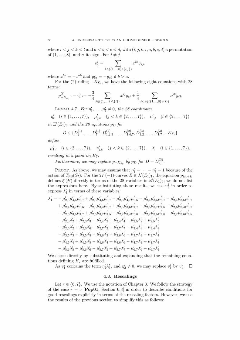
50 4. UNIVERSAL TORSORS AND HOMOGENEOUS SPACES
where i < j < k < l and a < b < c < d, with (i, j, k, l, a, b, c, d) a permutationof (1, . . . , 8), and σ its sign. For i 6= j
vij =
∑k∈({1,...,8}\{i,j})
xikykj ,
where xba = −xab and yba = −yab if b > a.For the (2)-ruling −KS7 , we have the following eight equations with 28
terms:
p(i)−KS7
:= vii := −3
4
∑j∈({1,...,8}\{i})
xijyij +14
∑j<k∈({1,...,8}\{i})
xjkyjk
Lemma 4.7. For η′1, . . . , η′7 6= 0, the 28 coordinates
η′i (i ∈ {1, . . . , 7}), µ′j,k (j < k ∈ {2, . . . , 7}), ν ′1,l (l ∈ {2, . . . , 7})
in Ξ′(E1)0 and the 28 equations pD for
D ∈ {D(1)2 , . . . , D
(1)7 , D
(2)1,2,3, . . . , D
(2)1,6,7, D
(3)1,2, . . . , D
(3)1,7,−KS7}
define
µ′1,i (i ∈ {2, . . . , 7}), ν ′j,k (j < k ∈ {2, . . . , 7}), λ′l (l ∈ {1, . . . , 7}),resulting in a point on H7.
Furthermore, we may replace p−KS7by pD for D = D
(3)2,1.
Proof. As above, we may assume that η′1 = · · · = η′7 = 1 because of theaction of TNS(S7). For the 27 (−1)-curves E ∈ N (E1)1, the equation pE1+E
defines ξ′(E) directly in terms of the 28 variables in Ξ′(E1)0; we do not listthe expressions here. By substituting these results, we use v1
1 in order toexpress λ′1 in terms of these variables:
λ′1 =− µ′2,3µ′4,5µ
′6,7 + µ′2,3µ
′4,6µ
′5,7 − µ′2,3µ
′4,7µ
′5,6 + µ′2,4µ
′3,5µ
′6,7 − µ′2,4µ
′3,6µ
′5,7
+ µ′2,4µ′3,7µ
′5,6 − µ′2,5µ
′3,4µ
′6,7 + µ′2,5µ
′3,6µ
′4,7 − µ′2,5µ
′3,7µ
′4,6 + µ′2,6µ
′3,4µ
′5,7
− µ′2,6µ′3,5µ
′4,7 + µ′2,6µ
′3,7µ
′4,5 − µ′2,7µ
′3,4µ
′5,6 + µ′2,7µ
′3,5µ
′4,6 − µ′2,7µ
′3,6µ
′4,5
− µ′2,3λ′2 + µ′2,3λ
′3 − µ′2,4λ
′2 + µ′2,4λ
′4 − µ′2,5λ
′2 + µ′2,5λ
′5
− µ′2,6λ′2 + µ′2,6λ
′6 − µ′2,7λ
′2 + µ′2,7λ
′7 − µ′3,4λ
′3 + µ′3,4λ
′4
− µ′3,5λ′3 + µ′3,5λ
′5 − µ′3,6λ
′3 + µ′3,6λ
′6 − µ′3,7λ
′3 + µ′3,7λ
′7
− µ′4,5λ′4 + µ′4,5λ
′5 − µ′4,6λ
′4 + µ′4,6λ
′6 − µ′4,7λ
′4 + µ′4,7λ
′7
− µ′5,6λ′5 + µ′5,6λ
′6 − µ′5,7λ
′5 + µ′5,7λ
′7 − µ′6,7λ
′6 + µ′6,7λ
′7
We check directly by substituting and expanding that the remaining equa-tions defining H7 are fulfilled.
As v21 contains the term η′2λ
′1, and η′2 6= 0, we may replace v1
1 by v21. �
4.3. Rescalings
Let r ∈ {6, 7}. We use the notation of Chapter 3. We follow the strategyof the case r = 5 [Pop01, Section 6.3] in order to describe conditions forgood rescalings explicitly in terms of the rescaling factors. However, we usethe results of the previous section to simplify this as follows:
4.3. RESCALINGS 51
LetM6 := {E1 + E | E ∈ N (E1)1}
and letM7 := {E1 + E | E ∈ N (E1)1} ∪ {D(3)
2,1}.
Let Hr ⊂ A′r be the variety defined by the equations gD for D ∈Mr.
By Proposition 4.4, Lemma 4.6, and Lemma 4.7, Hr ∩ Ur = Hr ∩ Ur.
Remark 4.8. Because of N (E1)2 = {C1}, it could be considered morenatural to use −KS7 = E1+C1 instead of D(3)
2,1 = E2+C1 in the definition ofM7. However, we choose to avoid the (2)-ruling −KS7 for technical reasons.
Lemma 4.9. A rescaling φr : Ar → A′r is good if and only if it embeds
A(Sr) into Hr.
Proof. As Hr ⊂ Hr, a good rescaling φr satisfies φr(A(Sr)) ⊂ Hr.Conversely, we have
φr(A(Sr)) ∩ Ur ⊂ Hr ∩ Ur = Hr ∩ Ur
by Lemma 4.6 and Lemma 4.7. Taking the closure and using that Hr
is closed and that A(Sr) is irreducible by Lemma 2.9, we conclude thatφr(A(Sr)) ⊂ Hr, so the rescaling is good. �
As in Theorem 3.2, let Jr be the ideal defining A(Sr) in Ar.In terms of the coordinate rings K[Ar] and K[A′
r] and in view of theprevious lemma, a rescaling φr is good if, for all D ∈ Mr, the ideal Jr ⊂rad(Jr) contains φ∗r(pD), where pD is the equation definingHr correspondingto the (1)-ruling D.
As K[Ar] and K[A′r] are both graded by Pic(Sr) and φ∗r respects this
grading, we need rescaling factors such that φ∗r(pD) of degree D ∈ Mr isa linear combination of the equations FD,1, . . . , FD,r−3 ∈ Jr. For concretecalculations in the next sections, we describe this more explicitly:
Let D ∈ Mr be a (1)-ruling, which can be written in r − 1 ways as thesum of two (−1)-curves E′
i, E′′i . For i ∈ {1, . . . , r − 1}, let
ξi := ξ(E′i)ξ(E
′′i ), ξ′i := ξ′(E′
i)ξ′(E′′
i ), ξ′′i := ξ′′(E′i)ξ
′′(E′′i ).
Then pD has the form
(4.1) pD =r−1∑i=1
εiξ′i
with εi ∈ {±1}.As ξi vanishes exactly on E′
i∪E′′i , the 2-dimensional space H0(Sr,O(D))
is generated by any two ξi, ξi′ . Hence, all other r − 3 elements ξj are linearcombinations of ξi, ξi′ , with non-vanishing coefficients. This gives r − 3relations of degree D in Cox(Sr). Rearranging ξ1, . . . , ξr−1 such that thetwo elements ξi, ξi′ of our choice have the indices r − 2 and r − 1, we canwrite them as
(4.2) FD,j = ξj + αjξr−2 + βjξr−1,
for j ∈ {1, . . . , r − 3}, where αj , βj ∈ K∗.

52 4. UNIVERSAL TORSORS AND HOMOGENEOUS SPACES
Suppose that φ∗r(pD) is a linear combination of the FD,j with factors λj :
φ∗r(pD)−r−3∑j=1
λjFD,j = 0.
Since φ∗r(ξ′(E)) = ξ′′(E) · ξ(E), we have φ∗r(ξ
′i) = ξ′′i · ξi for the monomials
of degree 2. Then the above equation is equivalent to the vanishing of
r−3∑i=1
(εiξ′′i −λi)ξi+
εr−2ξ′′r−2 −
r−3∑j=1
λjαj
ξr−2+
εr−1ξ′′r−1 −
r−3∑j=1
λjβj
ξr−1.
For i ∈ {1, . . . , r − 3}, we see by considering the coefficients of ξi thatwe must choose λi = εiξ
′′i . With this, consideration of the coefficients of
ξr−2 and ξr−1 results in the following conditions gD,1, gD,2 on the rescalingfactors ξ′′j , which are homogeneous of degree D ∈ Pic(Sr):
gD,1 := εr−2ξ′′r−2 −
r−3∑j=1
εjαjξ′′j = 0, gD,2 := εr−1ξ
′′r−1 −
r−3∑j=1
εjβjξ′′j = 0.
Note that our choice of ξr−2 and ξr−1 in the definition of FD,j as discussedbefore (4.2) is reflected here in the sense that gD,1 and gD,2 express thecorresponding ξ′′r−2 and ξ′′r−1 as linear combinations of ξ′′1 , . . . , ξ
′′r−3 with non-
zero coefficients.This information can be summarized as follows:
Lemma 4.10. For r ∈ {6, 7}, a rescaling is good if and only if therescaling factors ξ′′(E) fulfill the equations gD,1 and gD,2 for each (1)-rulingD ∈Mr.
As described above precisely, the non-zero coefficients εi are taken fromthe equations pD (4.1) defining Hr, and the non-zero αj, βj are taken fromthe equations FD,j (4.2) defining A(Sr).
Let Ξ′′(E)k (resp. Ξ′′(E)>k) be the set of all ξ′′(E′) for E′ ∈ N (E)k
(resp. E′ ∈ N (E)>k). Let
Ξ′′i,j := Ξ′′(E1)i ∩ Ξ′′(E2)j .
We claim that we may express the rescaling factors Ξ′′(E1)>0 ∪Ξ′′(E2)>0 interms of the other Nr−2 + 2 rescaling factors {η′′1 , η′′2} ∪ Ξ′′0,0.
We will prove this for r ∈ {6, 7} as follows: The 2 · (Nr − Nr−1 − 1)equations gD,i are homogeneous of degree D with respect to the Pic(Sr)-grading of the variables ξ′′(E), and we are interested only in the solutionswhere all ξ′′(E) are non-zero. Because of the action of TNS(Sr) on therescaling factors and as E1, . . . , Er are part of a basis of Pic(Sr), we mayassume η′′1 = · · · = η′′r = 1.
Consider a (1)-ruling D = E1 + E such that (E2, E) = 0. Then
D = E′1 + E′′
1 = · · · = E′r−3 + E′′
r−3 = E1 + E = E2 + E′
are the r − 1 possibilities to write D as the sum of two intersecting (−1)-curves. Here, E′
i, E′′i ∈ N (E1)0 ∩ N (E2)0. As in the discussion before
Lemma 4.10, we may set up the equations FD,j such that gD,1 and gD,2
express ξ′′(E) and ξ′′(E′) directly as a linear combination of ξ′′(E′i)ξ
′′(E′′i ).

4.4. DEGREE 3 53
This expresses all ξ(E) ∈ Ξ′′1,0 and all ξ′′(E′) ∈ Ξ′′0,1 in terms of variables inΞ′′0,0.
For a (1)-ruling D = E1 + E such that (E2, E) = 1, we have
D = E′1 + E′′
1 = · · · = E′r−2 + E′′
r−2 = E1 + E,
where we may assume (E2, E′i) = 0 and (E2, E
′′i ) = 1. Since (E1, E
′i) =
(E1, E′′i ) = 0, we have ξ′′(E′
i) ∈ Ξ′′0,0 and ξ′′(E′′i ) ∈ Ξ′′0,1. Using the previous
findings to express ξ′′(E′′i ) in terms of variables Ξ′′0,0, the equation gD,1 results
in a condition on the variables Ξ′′0,0, while gD,2 expresses ξ′′(E) ∈ Ξ′′1,1 interms of these variables.
In the case r = 7, the equation gD,2 for D = E1 + C2 expresses λ′′2 ∈Ξ′′1,2 in terms of variables in Ξ′′0,1, and gD,1 gives a further condition onthese variables. Furthermore, gD,2 for the (1)-ruling D = E2 +C1 expressesλ′′1 ∈ Ξ′′2,1 in terms of Ξ′′1,0, while gD,1 gives a further condition on them.Substituting the expressions for Ξ′′0,1 respectively Ξ′′1,0 in terms of Ξ′′0,0, weget expressions for λ′′2 and λ′′1, while the gD,1 result in further condition onΞ′′0,0.
We summarize this in the following lemma. For its proof, it remains toshow in the following sections that the expressions for Ξ′′(E1)>0 ∪Ξ′′(E2)>0
are non-zero, and that the further conditions vanish.
Lemma 4.11. We can write the Nr−Nr−2−2 rescaling factors in the setΞ′′(E1)>0∪Ξ′′(E2)>0 as non-zero expressions in terms of Nr−2 +2 rescalingfactors Ξ′′0,0 ∪ {ξ′′(E1), ξ′′(E2)}. With this, the Nr − 2Nr−1 + Nr−2 furtherconditions on the rescaling factors are trivial.
For an open subset of theNr−2+2 parameters {η′′1 , η′′2}∪Ξ′′0,0, all rescalingfactors are non-zero, so we obtain good rescalings, which proves Theorem 4.1once the proof of Lemma 4.11 is completed.
4.4. Degree 3
In this section, we prove Lemma 4.11 for r = 6 by solving the systemof equations on the rescaling factors of Lemma 4.10: For each (1)-rulingD ∈ M6, we determine the coefficients of the equation pD defining H6 asin (4.1), and find the coefficients αj , βj of FD,j defining A(S6) as in (4.2) inthe list in Section 3.3. This allows us to write down the 20 equations gD,i
on the rescaling factors ξ′′(E) explicitly. Let
γ1 := ad− bc, γ2 := (a− 1)(d− 1)− (b− 1)(c− 1)
for simplicity.
gE1+m1,2,1 = −η′′3µ′′2,3 − η′′4µ′′2,4 − bη′′5µ
′′2,5 − dη′′6µ
′′2,6,
gE1+m1,2,2 = η′′1µ′′1,2 + η′′4µ
′′2,4 + η′′5µ
′′2,5 + η′′6µ
′′2,6,
gE1+m1,3,1 = −η′′1µ′′1,3 + η′′4µ′′3,4 + η′′5µ
′′3,5 + η′′6µ
′′3,6,
gE1+m1,3,2 = η′′2µ′′2,3 + η′′4µ
′′3,4 + aη′′5µ
′′3,5 + cη′′6µ
′′3,6,
gE1+m1,4,1 = −η′′1µ′′1,4 + η′′3µ′′3,4 + (b− 1)η′′5µ
′′4,5 + (1− d)η′′6µ
′′4,6,
gE1+m1,4,2 = −η′′2µ′′2,4 + η′′3µ′′3,4 + (b− a)η′′5µ
′′4,5 + (c− d)η′′6µ
′′4,6,

54 4. UNIVERSAL TORSORS AND HOMOGENEOUS SPACES
gE1+m1,5,1 = −η′′2µ′′2,5 + a/bη′′3µ′′3,5 + (a− b)/bη′′4µ
′′4,5 + γ1/bη
′′6µ
′′5,6,
gE1+m1,5,2 = −η′′1µ′′1,5 + 1/bη′′3µ′′3,5 + (1− b)/bη′′4µ
′′4,5 + (d− b)/bη′′6µ
′′5,6,
gE1+m1,6,1 = −η′′1µ′′1,6 + 1/dη′′3µ′′3,6 + (d− 1)/dη′′4µ
′′4,6 + (b− d)/dη′′5µ
′′5,6,
gE1+m1,6,2 = −η′′2µ′′2,6 + c/dη′′3µ′′3,6 + (d− c)/dη′′4µ
′′4,6 − γ1/dη
′′5µ
′′5,6,
gE1+Q2,1 = a(c− d)η′′1λ′′2 + (d− 1)η′′2λ
′′1 − µ′′3,4µ
′′5,6 + µ′′3,6µ
′′4,5,
gE1+Q2,2 = γ1η′′1λ
′′2 + (b− d)η′′2λ
′′1 − µ′′3,5µ
′′4,6 − µ′′3,6µ
′′4,5,
gE1+Q3,1 = b(c− d)η′′1λ′′3 + (c− 1)η′′3λ
′′1 − µ′′2,4µ
′′5,6 + µ′′2,6µ
′′4,5,
gE1+Q3,2 = γ1η′′1λ
′′3 + (a− c)η′′3λ
′′1 − µ′′2,5µ
′′4,6 − µ′′2,6µ
′′4,5,
gE1+Q4,1 = bcη′′1λ′′4 + (bc− b− c+ 1)η′′4λ
′′1 − µ′′2,3µ
′′5,6 + µ′′2,6µ
′′3,5,
gE1+Q4,2 = (ad− bc)η′′1λ′′4 + γ2η
′′4λ
′′1 + µ′′2,5µ
′′3,6 − µ′′2,6µ
′′3,5,
gE1+Q5,1 = (d− c)η′′1λ′′5 + γ2η
′′5λ
′′1 − µ′′2,4µ
′′3,6 + µ′′2,6µ
′′3,4,
gE1+Q5,2 = cη′′1λ′′5 + (a− c)(1− b)η′′5λ
′′1 − µ′′2,3µ
′′4,6 − µ′′2,6µ
′′3,4,
gE1+Q6,1 = (b− a)η′′1λ′′6 + γ2η
′′6λ
′′1 + µ′′2,4µ
′′3,5 − µ′′2,5µ
′′3,4,
gE1+Q6,2 = aη′′1λ′′6 + (c− a)(d− 1)η′′6λ
′′1 − µ′′2,3µ
′′4,5 + µ′′2,5µ
′′3,4.
As explained in the previous section, we may assume η′′1 = · · · = η′′6 = 1.Recall the discussion before the definition (4.2) of FD,j and Lemma 4.10.
If we had chosen ξ4 = ηiλ1 and ξ5 = η1λi when writing down the equationsFE1+Qi,j in Section 3.3, then the resulting gE1+Qi,2 would give λ′′i directlyas a quadratic expression in terms of µ′′j,k. Furthermore, each of the fivegE1+Qi,1 would express λ′′1 as a quadratic equation in µ′′j,k. Of course, weget the same result by solving the equivalent system of equations gE1+Qi,j
as listed above.The equations gE1+m1,i,j for i ∈ {3, . . . , 6} and gE1+Q2,j allow us to
express the variables µ′′1,i, λ′′2 in Ξ′′1,0 and µ′′2,i, λ
′′1 in Ξ′′0,1 in terms of the
six variables µ′′3,4, . . . , µ′′5,6 ∈ Ξ′′0,0. (As we have set the remaining elements
η′′3 , . . . , η′′6 of Ξ′′0,0 to the value 1, they do not occur in these expressions.)
With γ3 := d(a− c)(1− b)− c(b− d)(1− a), we obtain:
µ′′1,3 =µ′′3,4 + µ′′3,5 + µ′′3,6,
µ′′2,3 =− µ′′3,4 − aµ′′3,5 − cµ′′3,6,
µ′′1,4 =µ′′3,4 + (b− 1)µ′′4,5 + (1− d)µ′′4,6,
µ′′2,4 =µ′′3,4 + (b− a)µ′′4,5 + (c− d)µ′′4,6,
µ′′1,5 =1/bµ′′3,5 + (1− b)/bµ′′4,5 + (d− b)/bµ′′5,6,
µ′′2,5 =a/bµ′′3,5 + (a− b)/bµ′′4,5 + γ1/bµ′′5,6,
µ′′1,6 =1/dµ′′3,6 + (d− 1)/dµ′′4,6 + (b− d)/dµ′′5,6,
µ′′2,6 =c/dµ′′3,6 + (d− c)/dµ′′4,6 − γ1/dµ′′5,6,
λ′′1 =− γ1/γ3µ′′3,4µ
′′5,6 − a(d− c)/γ3µ
′′3,5µ
′′4,6 − c(b− a)/γ3µ
′′3,6µ
′′4,5,
λ′′2 =(b− d)/γ3µ′′3,4µ
′′5,6 + (1− d)/γ3µ
′′3,5µ
′′4,6 + (1− b)/γ3µ
′′3,6µ
′′4,5.
We consider the remaining equations gE1+E,i for E ∈ {m1,2, Q3, . . . , Q6}.We can use gE1+E,2 and substitution of our previous results in order to

4.5. DEGREE 2 55
express ξ′′(E) ∈ Ξ′′1,1 in terms of Ξ′′0,0:
µ′′1,2 =µ′′3,4 − a/bµ′′3,5 − c/dµ′′3,6 + (a− b)(b− 1)/bµ′′4,5
+ (d− c)(d− 1)/dµ′′4,6 + (b− d)γ1/(bd)µ′′5,6,
λ′′3 =(a− c)/γ3µ′′3,4µ
′′5,6 + a(1− c)/(bγ3)µ′′3,5µ
′′4,6 + c(1− a)/(dγ3)µ′′3,6µ
′′4,5
+ 1/(bd)µ′′4,5µ′′4,6 − 1/dµ′′4,5µ
′′5,6 + 1/bµ′′4,6µ
′′5,6,
λ′′4 =γ2/γ3µ′′3,4µ
′′5,6 − 1/(bd)µ′′3,5µ
′′3,6 + (1− d)(c− d)(a− 1)/(dγ3)µ′′3,5µ
′′4,6
− 1/dµ′′3,5µ′′5,6 + (1− c)(b− 1)(a− b)/(bγ3)µ′′3,6µ
′′4,5 − 1/bµ′′3,6µ
′′5,6,
λ′′5 =1/dµ′′3,4µ′′3,6 − 1/dµ′′3,4µ
′′4,6 + (b− d)(1− a)γ1/(dγ3)µ′′3,4µ
′′5,6
+ aγ2/γ3µ′′3,5µ
′′4,6 + (b− 1)(a− b)(a− c)/γ3µ
′′3,6µ
′′4,5 − µ′′3,6µ
′′4,6,
λ′′6 =− 1/bµ′′3,4µ′′3,5 − 1/bµ′′3,4µ
′′4,5 + (1− c)(b− d)γ1/(bγ3)µ′′3,4µ
′′5,6
− µ′′3,5µ′′4,5 + (d− 1)(c− d)(a− c)/γ3µ
′′3,5µ
′′4,6 + cγ2/γ3µ
′′3,6µ
′′4,5
Finally, we check by substituting and expanding that the five further condi-tions gE1+E,1 are trivial.
Using the restrictions on a, b, c, d imposed by the fact that p1, . . . , p6 arein general position (e.g., a must be different from b and c, and all are neither0 nor 1), we see that µ′′1,2, . . . , µ
′′2,6, λ
′′1, . . . , λ
′′6 are non-zero polynomials in
µ′′3,4, . . . , µ′′5,6. Therefore, for an open subset of the N4 + 2 = 12 parameters
η′′1 , . . . , η′′6 , µ
′′3,4, . . . , µ
′′5,6, all rescaling factors are non-zero, resulting in good
rescalings.
4.5. Degree 2
For the proof of Lemma 4.11 for r = 7, we proceed as in the case r = 6and assume η′′1 = · · · = η′′7 = 1.
Let D := D(1)i ∈ M7 for i ∈ {3, . . . , 7}. We can arrange FD,1, . . . FD,4
in such a way that gD,1 and gD,2 express µ′′1,i and µ′′2,i in terms of µ′′i,j forj ∈ {3, . . . , 7} \ {i} (see the discussion before Lemma 4.10). Similarly, fori ∈ {3, . . . , 7} and D := D
(2)1,2,i ∈ M7, we can arrange gD,1 and gD,2 such
that they express ν ′′1,i and ν ′′2,i linearly in ν ′′1,2 and of degree 2 in µ′′3,4, . . . , µ′′6,7.
This expresses all variables in Ξ′′0,1 ∪ Ξ′′1,0 in terms of Ξ′′0,0.
Substituting this into an appropriately arranged gD,2 for D := D(1)2 ∈
M7 gives µ′′1,2 ∈ Ξ′′1,1 in terms of µ′′3,4, . . . , µ′′6,7, and we check that gD,1
becomes trivial.Now, let D := D
(2)1,i,j ∈ M7 for i < j ∈ {3, . . . , 7}. We arrange gD,1
and gD,2 such that they express ν ′′1,i respectively ν ′′i,j in terms of ν ′′1,j andexpressions of degree 2 in µ′′k,l. Using our previous findings, the first ex-pression turns out trivial, and the second one gives ν ′′i,j ∈ Ξ′′1,1 in terms ofν ′′1,2, µ
′′3,4, . . . , µ
′′6,7 ∈ Ξ′′0,0.
Finally, let D ∈ {D(3)1,2, . . . , D
(3)1,7, D
(3)2,1} ⊂ M7. We arrange gD,1 and gD,2
such that the first one is an expression in µ′′j,k and ν ′′j,k which becomes trivial.The second one expresses λ′′i in terms of µ′′j,k and ν ′′j,k, and we substitute againour previous results.
56 4. UNIVERSAL TORSORS AND HOMOGENEOUS SPACES
This completes the proof of Lemma 4.11 and thus Theorem 4.1. Intotal, we obtain good rescalings for an open subset of a system N5 + 2 = 18parameters
η′′1 , . . . , η′′7 , µ′′3,4, . . . , µ
′′6,7, ν ′′1,2.
Since it is straightforward to determine the exact expressions for the re-maining 38 rescaling factors in terms of these parameters, and since theexpressions are rather long, we choose not to list them here.
Remark 4.12. In principle, it would be possible to consider the condi-tions gD,i for all (1)-rulings without reducing to the subset Mr as we didin Section 4.2. While this is doable in degree 3 with some software help(Magma), especially the expressions corresponding to the (1)-ruling D(5)
i indegree 2 seem to be out of reach for direct computations. Furthermore, wewould have to embed the relations vi
i corresponding to the (2)-ruling −KS7 ,which causes further complications.
Remark 4.13. For r ∈ {5, 6, 7}, there is a (Nr−2 − r + 1)-parameterfamily of images of A(Sr) under good embeddings in Hr by Remark 4.2.The dimension of A(Sr) is r+3, and there is a (2 · (r−4))-parameter familyof smooth Del Pezzo surfaces Sr of degree 9 − r. The dimension of Hr isNr−1 + 1.
In fact, [Pop01, Section 6.3] shows that the closure of the union of allthese images for all Del Pezzo surfaces of degree 4 equals H5.
For r = 6, by comparing the dimensions and numbers of parameters, asimilar result seems possible. However, for r = 7, we have
(Nr−2 − r + 1) + (r + 3) + 2 · (r − 4) = 26,
while H7 has dimension Nr−1 + 1 = 28. Consequently, the closure of theunion of the corresponding images, over all Del Pezzo surfaces of degree 2,under all good embeddings cannot be H7 for dimension reasons.

CHAPTER 5
Universal torsors which are hypersurfaces
5.1. Introduction
The universal torsor of a generalized Del Pezzo surface S has one of thefollowing three types (Lemma 2.13):
• The universal torsor can be presentable as a Zariski open subsetof affine space. By Lemma 2.12 and Proposition 2.10, this is trueexactly when S is toric.
• The universal torsor can be a Zariski open subset of a hypersurfacein affine space.
• In other cases, the universal torsor is more complicated: It can bean open subset of an affine variety that has codimension ≥ 2 inaffine space.
We focus on universal torsors of the second type. A first example, theuniversal torsor over a cubic surface of type E6, has been worked out byHassett and Tschinkel [HT04].
Universal torsors are closely connected to the Cox rings of Del Pezzosurfaces (Chapter 2). By Lemma 2.13, the question which of the three casesabove a universal torsor belongs to is equivalent to the question whether theCox ring with a minimal set of homogeneous generators (cf. Lemma 2.5) is apolynomial ring without relations, with one relation up to scalar multiples,or with more relations.
In this chapter, we determine for all types of generalized Del Pezzo sur-faces of degree ≥ 3 what kind of Cox ring they have (cf. Table 5.1). Ourresults were first made available as [Der06c].
degree toric one relation more than one relation9 P2 – –8 2 smooth, 1 singular – –7 1 smooth, 1 singular – –6 1 smooth, 3 singular 2 singular –5 2 singular 4 singular 1 smooth4 3 singular 7 singular 1 smooth, 5 singular3 1 singular 7 singular 1 smooth, 12 singular
Table 5.1. Relations in Cox rings of Del Pezzo surfaces
Theorem 5.1. The Cox rings of generalized Del Pezzo surfaces whosedegree is at least 3 have the following properties:
• In degree at least 7, all generalized Del Pezzo surfaces are toric.
57
58 5. UNIVERSAL TORSORS WHICH ARE HYPERSURFACES
• In degree 6, two types A1 (with three lines), A2 have a Cox ringwith 7 generators and one relation. The smooth and three types A1
(with four lines), 2A1, A2 + A1 are toric.• In degree 5, four types A1, A2, A3, A4 have a Cox ring with 8
generators and one relation. The smooth surface has a Cox ringwith more generators and relations, and two types 2A1, A2 + A1
are toric.• In degree 4, seven types 3A1, A2+A1, A3 (with five lines), A3+A1,
A4, D4, D5 have a Cox ring with 9 generators and one relation.The smooth surface and five types A1, 2A1 (with eight or ninelines), A2, A3 (with four lines) have a Cox ring with more gener-ators and relations, and three types 4A1, A2 + 2A1, A3 + 2A1 aretoric.
• In degree 3, seven types D4, A3 + 2A1, 2A2 + A1, A4 + A1, D5,A5 + A1, E6 have a Cox ring with 10 generators and one relation.The smooth surface and 12 types A1, 2A1, A2, 3A1, A2 +A1, A3,4A1, A2 +2A1, A3 +A1, 2A2, A4, A5 have a Cox ring with moregenerators and relations, and the type 3A2 is toric.
In Section 5.2, we describe the steps which must be taken to calculatethe Cox ring of each generalized Del Pezzo surface S explicitly in case thereis exactly one relation in Cox(S).
In Sections 5.3, 5.4, 5.5, and 5.6, we check for every type of degree≥ 3 which of the three cases it belongs to. For each type with exactlyone relation, we calculate the Cox ring, and we list the data which is mostimportant for its calculation and applications: We give a “nice”model whichis defined over Q, its singularities, its lines (which are defined over Q),generators of the Picard group, the effective cone, generators of the Coxring, the extended Dynkin diagram, and the map from the universal torsorto the Del Pezzo surface.
5.2. Strategy of the proofs
In this section, we give an overview of the method of Hassett and Tschin-kel [HT04] to calculate the Cox ring of generalized Del Pezzo surfaces incases where the Cox ring has exactly one relation.
By Lemma 2.7, the Cox ring has one generating section for every negativecurve. In some cases, the Cox ring is generated by these sections, but thisis not always true. In that case, we look for extra generators in nef degrees(Lemma 2.8). When we find enough generators, we have a relation whichcan be calculated explicitly once we know details about the anticanonicalembedding.
In more detail, we perform the following steps: Let S be a smooth orsingular Del Pezzo surface of degree 9 − r ≥ 3, given by the vanishing ofsome homogeneous polynomials for its anticanonical embedding into P9−r.Let S be its minimal desingularization. We apply this method only in thecases where the Cox ring will turn out to have exactly r+ 4 generators andone relation. In the other cases, it would fail.
Find the extended Dynkin diagram of the negative curves. Forthis, first we search for the lines on S, by looking at the equations of the
5.2. STRATEGY OF THE PROOFS 59
anticanonical embedding of S (Remark 1.26). Using the classifications of[BW79] for degree 3 and [CT88] for degrees ≥ 4, we know when we aredone. Then we determine the singularities, resolve them by blow-ups, andkeep track of the intersection behavior of the exceptional divisors with thetransforms of the lines. This must be done explicitly for degree 3, andthe results can be found in [CT88] for degrees ≥ 4. The information issummarized in an extended Dynkin diagram of negative curves. Note thatthe diagrams can also be constructed from the information given in [AN04,Table 3], as explained in Section 1.4.
Determine a basis of the Picard group. We need a Z-basis forPic(S) ∼= Zr+1: We test for different (r+ 1)-element subsets of the negativecurves whether their intersection matrix has determinant ±1. Once we havefound such a subset, we call its elements E1, . . . , Er+1, and the remainingnegative curves are called Er+2, . . . , Et. By considering their intersectionwith the basis, we determine Er+2, . . . , Et in terms of this basis. Using theadjunction formula, we calculate the anticanonical class −KeS , which is nefsince it describes the anticanonical embedding of S.
Determine the effective cone and its dual, the nef cone. In everycase, we want to show that the effective cone is generated by the negativecurves E1, . . . , Et. Arguing as in [HT04, Proposition 3.5], we only needto check that the cone generated by E1, . . . , Et contains its dual, which isgenerated by some divisors A1, . . . , Au. This can be done by an explicitcalculation using the basis we found in the previous step. It turns out to betrue in every case. We will show this result in general in Proposition 8.11.Therefore, A1, . . . , Au generate the nef cone. By Lemma 2.7, a generatingset of Cox(S) must contain a non-zero section ηi ∈ H0(Ei) for every i ∈{1, . . . , t}.
Find generating sections in degrees of generators of the nefcone. To every Ai, we can associate a map from S to projective space. Bylooking at these maps carefully, we can find extra generators αi ∈ H0(Ai) ofthe Cox ring. We obtain generators η1, . . . , ηt, α1, . . . , αs, where t+s = r+4,which fulfill a certain relation. Assuming that this is a generating set withone relation, we check that this gives exactly the right number of independentsections in each H0(Ai), where dimH0(Ai) = χ(Ai) can be calculated usingRiemann-Roch and Kawamata-Viehweg as in [HT04, Corollary 1.10].
Determine φ∗(xi) for the anticanonical embedding. Especially byconsidering projections from the singularities and lines on the one hand, andmaps to P2 corresponding to the fact that S is a blow-up of P2 in r pointson the other hand, and by considering the corresponding transformations ofthe extended Dynkin diagrams, we find out which projections
ψi : x 7→ (xj1 : · · · : xjn)
are given by Ai, and what ψ∗i (xjl) ∈ H0(Ai) is. Finally, we combine this
information in order to get φ∗(xi) ∈ H0(−KeS) for
φ : S → S ↪→ P9−r.
Using the equations defining S, we derive a relation R from this. Note thateven though S might be defined by more than one equation, this gives only

60 5. UNIVERSAL TORSORS WHICH ARE HYPERSURFACES
one relation in the cases we consider. We obtain a map
% : K[η1, . . . , ηt, α1, . . . , αs]/(R) → Cox(S).
Prove injectivity of %. The argument is the same as in [HT04, The-orem 3.8]. We must check that −KeS is in the inner of the effective cone.
Prove surjectivity of %. We follow the proof of [HT04, Propo-sition 3.9]. We need to check that the generators of the effective coneA1, . . . , Au are contained in the moving cone corresponding to the r + 4divisors E1, . . . , Et, A1, . . . , As (cf. [HT04, Lemma 3.11]). Furthermore, wecheck that
t∑i=1
Ei +s∑
j=1
Ai = deg(R) +A
for some nef divisor A (cf. [HT04, Proposition 3.12]).
Remark 5.2. For many Del Pezzo surfaces S, the number of negativecurves on its minimal desingularization S is at least r + 5, so Lemma 2.7and Lemma 2.13 imply that Cox(S) has at least two relations.
On the other hand, in many cases where the number of negative curveson S is at most r + 4, the surfaces turn out to be toric or to have exactlyone relation in Cox(S).
However, S may have r + 4 or fewer negative curves, but two or morerelations (see Proposition 5.6 for type viii of degree 4, and Proposition 5.7for types xi and xvi of degree 3). In these cases, more work must be doneto see that the number of relations is actually at least two.
In the next sections, we go through all types of Del Pezzo surfaces ofdegrees ≥ 3 whose Cox rings have exactly one relation, and list the followinginformation for one example of each type:
• Equations for the anticanonical embedding are given. We choose“nice” equations in the sense that they are defined over Z, all thecoefficients are ±1, and the singularities and lines have“nice” forms.For applications, it can be useful to know these equations.
• The equations of the singularities and lines on the anticanonicalembedding are given, as we need their names Ei later. Furthermore,they are needed in applications.
• The ordering of the Ei is chosen in such a way that E1, . . . , Er+1
are a Z-basis of Pic(S). We list the other Ei and −KeS in terms ofthis basis, as this is needed for further calculations.
• We list generators and the relation of Cox(S). Here, ηi is always anon-zero section of H0(Ei), which is unique up to a scalar factor.For each extra generator αi, we give the degree in terms of ourbasis of Pic(S), specify which projection ψi : x 7→ (xj1 : · · · : xjn) itdefines, and what αi = ψ∗i (xjl
) and the corresponding divisor Ai is.We also describe the image of Ai under the projection ψ : S → S.We give the equation and the degree of the relation.
• We give the extended Dynkin diagram of the negative curves as inExample 1.27, and we also include the divisors A1, . . . , As (wherean edge means in this chapter that the intersection number is ≥ 1).
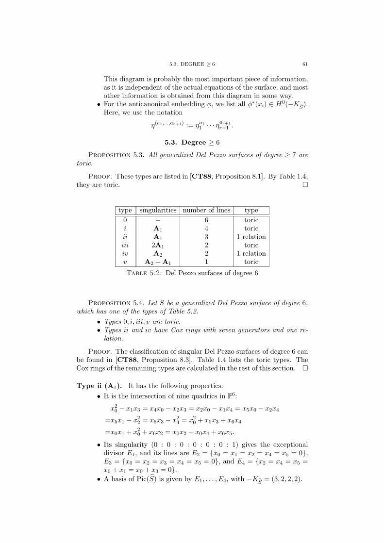
5.3. DEGREE ≥ 6 61
This diagram is probably the most important piece of information,as it is independent of the actual equations of the surface, and mostother information is obtained from this diagram in some way.
• For the anticanonical embedding φ, we list all φ∗(xi) ∈ H0(−KeS).Here, we use the notation
η(a1,...,ar+1) := ηa11 · · · ηar+1
r+1 .
5.3. Degree ≥ 6
Proposition 5.3. All generalized Del Pezzo surfaces of degree ≥ 7 aretoric.
Proof. These types are listed in [CT88, Proposition 8.1]. By Table 1.4,they are toric. �
type singularities number of lines type0 − 6 torici A1 4 toricii A1 3 1 relationiii 2A1 2 toriciv A2 2 1 relationv A2 + A1 1 toric
Table 5.2. Del Pezzo surfaces of degree 6
Proposition 5.4. Let S be a generalized Del Pezzo surface of degree 6,which has one of the types of Table 5.2.
• Types 0, i, iii, v are toric.• Types ii and iv have Cox rings with seven generators and one re-
lation.
Proof. The classification of singular Del Pezzo surfaces of degree 6 canbe found in [CT88, Proposition 8.3]. Table 1.4 lists the toric types. TheCox rings of the remaining types are calculated in the rest of this section. �
Type ii (A1). It has the following properties:• It is the intersection of nine quadrics in P6:
x20 − x1x3 = x4x0 − x2x3 = x2x0 − x1x4 = x5x0 − x2x4
=x5x1 − x22 = x5x3 − x2
4 = x20 + x0x3 + x6x4
=x0x1 + x20 + x6x2 = x0x2 + x0x4 + x6x5.
• Its singularity (0 : 0 : 0 : 0 : 0 : 0 : 1) gives the exceptionaldivisor E1, and its lines are E2 = {x0 = x1 = x2 = x4 = x5 = 0},E3 = {x0 = x2 = x3 = x4 = x5 = 0}, and E4 = {x2 = x4 = x5 =x0 + x1 = x0 + x3 = 0}.
• A basis of Pic(S) is given by E1, . . . , E4, with −KeS = (3, 2, 2, 2).

62 5. UNIVERSAL TORSORS WHICH ARE HYPERSURFACES
• The Cox ring is
Cox(S) = K[η1, . . . , η4, α1, α2, α3]/(η2α1 + η3α2 + η4α3),
where the degree of the relation is (1, 1, 1, 1), and deg(α1) = A1 =(1, 0, 1, 1) = ψ∗({(0 : 0 : 0 : a2 : ab : b2 : 0)}), deg(α2) = A2 =(1, 1, 0, 1) = ψ∗({(0 : a2 : ab : 0 : 0 : b2 : 0) | x1x5 − x2
2 = 0}), anddeg(α3) = A3 = (1, 1, 1, 0) = ψ∗({(a2 : −a2 : ab : −a2 : −ab : −b2 :0)}), where ψ is the projection S → S.
• The extended Dynkin diagram is:
A1
AAAA
AAAA
E2
BBBB
BBBB
A2 E3GFED@ABCE1
A3
}}}}}}}}E4
||||||||
Here, the divisors A1, A2, A3 meet in (0 : 0 : 0 : 0 : 0 : 1 : 0).• The anticanonical embedding is given by
(φ∗(xi)) = (η(1,1,1,0)α1α2, η(1,2,0,0)α2
1, η(2,2,1,1)α1, η
(1,0,2,0)α22,
η(2,1,2,1)α2, η(3,2,2,2), α1α2α3),
and furthermore, φ∗(−x0 − x1) = η(1,1,0,1)α1α3, φ∗(−x0 − x3) =η(1,0,1,1)α2α3, φ∗(−x2 − x4) = η(2,1,1,2)α3, and φ∗(2x0 + x1 + x3) =η(1,0,0,2)α2
3.
Type iv (A2). This surface has the following properties:• It is the intersection of the following nine quadrics in P6:
x0x5 − x3x4 = x0x6 − x1x4 = x0x6 − x2x3 = x3x6 − x1x5
=x4x6 − x2x5 = x1x6 + x23 + x3x4 = x2x6 + x3x4 + x2
4
=x26 + x3x5 + x4x5 = x1x2 + x0x3 + x0x4 = 0.
• Its singularity (1 : 0 : 0 : 0 : 0 : 0 : 0) gives the exceptional divisorsE1, E2, and its lines are E3 = {x2 = x3 = x4 = x5 = x6 = 0} andE4 = {x1 = x3 = x4 = x5 = x6 = 0}.
• A basis of Pic(S) is given by E1, . . . , E4, with −KeS = (4, 2, 3, 3).• The Cox ring is
Cox(S) = K[η1, . . . , η4, α1, α2, α3]/(η2α21 + η3α2 + η4α3),
where the relation is of degree (2, 1, 2, 2), and deg(α1) = A1 =(1, 0, 1, 1) = ψ∗({(a2 : 0 : 0 : ab : −ab : b2 : 0)}) gives the projectionψ1 : x 7→ (x5 : x6) with α1 = φ∗(x6), deg(α2) = A2 = (2, 1, 1, 2) =ψ∗({(0 : 0 : a3 : −a2b : b3 : −ab2)}) gives the projection ψ2 : x 7→(x3 : x5 : x6) with α2 = ψ∗2(x3), and deg(α3) = A3 = (2, 1, 2, 1) =ψ∗({(0 : a3 : 0 : −a2b : 0 : b3 : −ab2)}) gives the projectionψ3 : x 7→ (x4 : x5 : x6) with α3 = ψ∗3(x4).

5.4. DEGREE 5 63
• The extended Dynkin diagram is:
A2
AAAA
AAAA
E3
CCCC
CCCC
C
A1GFED@ABCE2
GFED@ABCE1
A3
}}}}}}}}E4
{{{{{{{{{
Here, A1, A2, A3 meet in (0 : 0 : 0 : 0 : 0 : 1 : 0).• The anticanonical embedding is given by
(φ∗(xi)) = (α2α3, η(1,1,1,0)α1α2, η
(1,1,0,1)α1α3,
η(2,1,2,1)α2, η(2,1,1,2)α3, η
(4,2,3,3), η(3,2,2,2)α1),
and furthermore, φ∗(−x1 − x2) = η(1,2,0,0)α31 and φ∗(−x3 − x4) =
η(2,2,1,1)α21.
5.4. Degree 5
By [CT88, Proposition 8.4], Table 5.3 lists all types of Del Pezzo surfacesof degree 5.
type singularities number of lines type0 − 10 ≥ 2 relationsi A1 7 1 relationii 2A1 5 toriciii A2 4 1 relationiv A2 + A1 3 toricv A3 2 1 relationvi A4 1 1 relation
Table 5.3. Del Pezzo surfaces of degree 5
Proposition 5.5. The generalized Del Pezzo surfaces of degree 5 ofTable 5.3 can be divided into the following groups:
• Type 0 has a Cox ring with 10 generators and five relations.• Types ii and iv are toric.• Types i, iii, v, vi have a Cox ring with 9 generators and one relation.
Proof. Type 0 has 10 negative curves. By Lemma 2.7, Cox(S) hasat least 10 generators. By Lemma 2.13, this implies that there is morethan one relation in Cox(S). More information on this surface can be foundin [Sko93], [Has04, Section 2.2], [Bre02]. The toric types are listed inTable 1.4.
For the other types, we calculate the Cox ring in what follows, and wesee that each of them has exactly one relation. �
Type i (A1). The surface of type i has the properties:
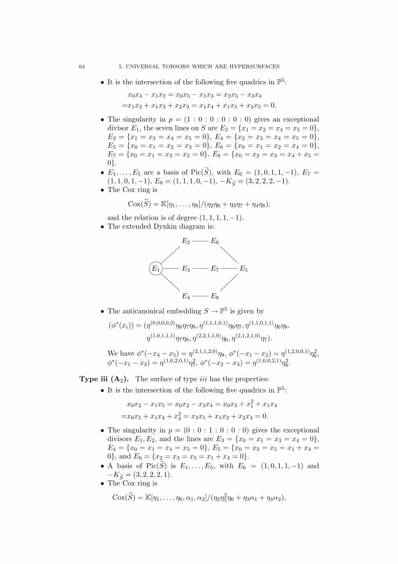
64 5. UNIVERSAL TORSORS WHICH ARE HYPERSURFACES
• It is the intersection of the following five quadrics in P5:
x0x4 − x1x2 = x0x5 − x1x3 = x2x5 − x3x4
=x1x2 + x1x3 + x2x3 = x1x4 + x1x5 + x2x5 = 0.
• The singularity in p = (1 : 0 : 0 : 0 : 0 : 0) gives an exceptionaldivisor E1, the seven lines on S are E2 = {x1 = x2 = x4 = x5 = 0},E3 = {x1 = x3 = x4 = x5 = 0}, E4 = {x2 = x3 = x4 = x5 = 0},E5 = {x0 = x1 = x2 = x3 = 0}, E6 = {x0 = x1 = x2 = x4 = 0},E7 = {x0 = x1 = x3 = x5 = 0}, E8 = {x0 = x2 = x3 = x4 + x5 =0}.
• E1, . . . , E5 are a basis of Pic(S), with E6 = (1, 0, 1, 1,−1), E7 =(1, 1, 0, 1,−1), E8 = (1, 1, 1, 0,−1), −KeS = (3, 2, 2, 2,−1).
• The Cox ring is
Cox(S) = K[η1, . . . , η8]/(η2η6 + η3η7 + η4η8),
and the relation is of degree (1, 1, 1, 1,−1).• The extended Dynkin diagram is:
E2 E6
@@@@
@@@@
GFED@ABCE1
||||||||
BBBB
BBBB
E3 E7 E5
E4 E8
~~~~~~~~
• The anticanonical embedding S → P5 is given by
(φ∗(xi)) = (η(0,0,0,0,2)η6η7η8, η(1,1,1,0,1)η6η7, η
(1,1,0,1,1)η6η8,
η(1,0,1,1,1)η7η8, η(2,2,1,1,0)η6, η
(2,1,2,1,0)η7).
We have φ∗(−x4 − x5) = η(2,1,1,2,0)η8, φ∗(−x1 − x2) = η(1,2,0,0,1)η26,
φ∗(−x1 − x3) = η(1,0,2,0,1)η27, φ
∗(−x2 − x3) = η(1,0,0,2,1)η28.
Type iii (A2). The surface of type iii has the properties:
• It is the intersection of the following five quadrics in P5:
x0x2 − x1x5 = x0x2 − x3x4 = x0x3 + x21 + x1x4
=x0x5 + x1x4 + x24 = x3x5 + x1x2 + x2x4 = 0.
• The singularity in p = (0 : 0 : 1 : 0 : 0 : 0) gives the exceptionaldivisors E1, E2, and the lines are E3 = {x0 = x1 = x3 = x4 = 0},E4 = {x0 = x1 = x4 = x5 = 0}, E5 = {x0 = x3 = x5 = x1 + x4 =0}, and E6 = {x2 = x3 = x5 = x1 + x4 = 0}.
• A basis of Pic(S) is E1, . . . , E5, with E6 = (1, 0, 1, 1,−1) and−KeS = (3, 2, 2, 2, 1).
• The Cox ring is
Cox(S) = K[η1, . . . , η6, α1, α2]/(η2η25η6 + η3α1 + η4α2),

5.4. DEGREE 5 65
where deg(α1) = A1 = (1, 1, 0, 1, 1) = ψ∗({(a2 : 0 : ab : 0 : 0 :−b2)}), deg(α2) = A2 = (1, 1, 1, 0, 1) = ψ∗({(a2 : ab : 0 : −b2 : 0 :0)}), and the degree of the relation is (1, 1, 1, 1, 1).
• The extended Dynkin diagram is:
A1
AAAA
AAAA
E3
CCCC
CCCC
C
E6 E5GFED@ABCE2
GFED@ABCE1
A2
~~~~~~~~E4
{{{{{{{{{
Here, A1, A2, E6 meet in (1 : 0 : 0 : 0 : 0 : 0).• The anticanonical embedding φ : S → P5 is given by
(φ∗(xi)) = (η(3,2,2,2,1), η(2,1,2,1,0)α1, η6α1α2,
η(1,1,1,0,1)η6α1, η(2,1,1,2,0)α2, η
(1,1,0,1,1)η6α2),
and furthermore, φ∗(−x1 − x4) = η(2,2,1,1,2)η6 and φ∗(−x3 − x5) =η(1,2,0,0,3)η2
6.
Type v (A3). The surface of type v has the following properties:• It is the intersection of the following five quadrics in P5:
x0x2 − x21 = x0x3 − x1x4 = x2x4 − x1x3
=x2x4 + x24 + x0x5 = x2x3 + x3x4 + x1x5 = 0.
• The singularity is in p = (0 : 0 : 0 : 0 : 0 : 1), giving threeexceptional divisors E1, E2, E3. The lines E4 = {x0 = x1 = x2 =x4 = 0} and E5 = {x0 = x1 = x3 = x4 = 0} intersect in p.
• A basis of Pic(S) is E1, . . . , E5, with −KeS = (2, 4, 3, 2, 3).• The Cox ring is
Cox(S) = K[η1, . . . , η5, α1, α2, α3]/(η1α21 + η3η
24α2 + η5α3),
where deg(α1) = A1 = (0, 1, 1, 1, 1) = ψ∗({(a2 : 0 : 0 : 0 : ab :−b2)}), deg(α2) = A2 = (1, 2, 1, 0, 2) = ψ∗({(a2 : ab : b2 : 0 : 0 :0)}), deg(α3) = A3 = (1, 2, 2, 2, 1) = ψ∗({(a3 : a2b : ab2 : −b3 :−ab2 : 0)}), and the degree of the relation is (1, 2, 2, 2, 2).
• The extended Dynkin diagram is:
A1
����
����
GFED@ABCE1
BBBB
BBBB
B
A2
????
????
A3 E5GFED@ABCE2
E4GFED@ABCE3
|||||||||
Here, A1, A2, A3 meet in (1 : 0 : 0 : 0 : 0 : 0).

66 5. UNIVERSAL TORSORS WHICH ARE HYPERSURFACES
• The anticanonical embedding φ : S → P5 is given by
(φ∗(xi)) = (η(2,4,3,2,3), η(2,3,2,1,2)α1, η(2,2,1,0,1)α2
1,
η(1,1,1,1,0)α1α2, η(1,2,2,2,1)α2, α2α3),
and furthermore, φ∗(−x2 − x4) = η(1,2,1,0,2)α3.
Type vi (A4). The surface of type vi has the following properties:• It is given by the intersection of the following five quadrics in P5:
x0x2 − x21 = x0x3 − x1x4 = x2x4 − x1x3
=x1x2 + x24 + x0x5 = x2
2 + x3x4 + x1x5 = 0.
• The singularity is p = (0 : 0 : 0 : 0 : 0 : 1), giving four exceptionaldivisors E1, . . . , E4 in Pic(S), and the line is E5 = {x0 = x1 = x2 =x4 = 0}.
• A basis of Pic(S) is E1, . . . , E5, with −KeS = (2, 4, 6, 3, 5).• The Cox ring is
Cox(S) = K[η1, . . . , η5, α1, α2, α3]/(η21η2α
31 + η4α
22 + η5α3),
where deg(α1) = A1 = (0, 1, 2, 1, 2) = ψ∗({(a2 : 0 : 0 : 0 : ab :−b2)}), deg(α2) = A2 = (1, 2, 3, 1, 3) = ψ∗({(a3 : a2b : ab2 : 0 : 0 :−b3)}), deg(α3) = A3 = (2, 4, 6, 3, 5) = −KeS = ψ∗({(a5 : −a3b2 :ab4 : −b5 : a2b3 : 0)}). The degree of the relation is (2, 4, 6, 3, 6).
• The extended Dynkin diagram is:
A2
~~~~
~~~~
~GFED@ABCE4
BBBB
BBBB
B
A1
@@@@
@@@@
@ A3 E5GFED@ABCE3
GFED@ABCE1GFED@ABCE2
|||||||||
Here, A1, A2, A3 meet in (1 : 0 : 0 : 0 : 0 : 0).• The anticanonical embedding φ : S → P5 is given by
(φ∗(xi)) = (η(2,4,6,3,5), η(2,3,4,2,3)α1, η(2,2,2,1,1)α2
1,
η(1,1,1,1,0)α1α2, η(1,2,3,2,2)α2, α3).
5.5. Degree 4
By Remark 1.13 and Remark 1.26, quartic Del Pezzo surfaces are certainintersections of two conics in P4. The extended Dynkin diagrams of theirlines and exceptional divisors can be found in [CT88, Proposition 6.1].
Proposition 5.6. The 16 types of generalized Del Pezzo surfaces ofdegree 4 of Table 5.4 can be divided into the following three groups:
• Types ix, x, xiv are toric.• The Cox rings of types v, vi, vii, xi, xii, xiii, xv have 9 generators
and one relation.

5.5. DEGREE 4 67
type singularities number of lines type0 − 16 ≥ 2 relationsi A1 12 ≥ 2 relationsii 2A1 9 ≥ 2 relationsiii 2A1 8 ≥ 2 relationsiv A2 8 ≥ 2 relationsv 3A1 6 1 relationvi A2 + A1 6 1 relationvii A3 5 1 relationviii A3 4 ≥ 2 relationsix 4A1 4 toricx A2 + 2A1 4 toricxi A3 + A1 3 1 relationxii A4 3 1 relationxiii D4 2 1 relationxiv A3 + 2A1 2 toricxv D5 1 1 relation
Table 5.4. Del Pezzo surfaces of degree 4
• The Cox rings of types 0, i, ii, iii, iv, viii have at least 10 generatorsand at least two independent relations.
Proof. The toric types ix, x, xiv are identified using Table 1.4. Fortypes 0, i, ii, iii, iv, the number of negative curves is greater than r+ 4 = 9,so Cox(S) has more than 9 generators by Lemma 2.7. Therefore, there mustbe more than one relation.
For type viii, this is not as obvious because it has only 7 negative curves.We can derive the following information from the extended Dynkin diagramof negative curves given in [CT88, Proposition 6.1]:
• The singularity gives the exceptional divisors E1, E2, E3, and theyintersect the four lines E4, . . . , E7 in the following way:
E6GFED@ABCE1
GFED@ABCE2GFED@ABCE3
BBBB
BBBB
E4
E7
||||||||E5
• A basis of Pic(S) is E1, . . . , E6, with E7 = (−1, 0, 1, 1, 1,−1) and−KeS = (1, 2, 3, 2, 2, 0).
• Four of the ten generators of the nef cone are B1 = (1, 1, 1, 0, 1, 1),B2 = (1, 1, 1, 1, 0, 1), B3 = (0, 1, 2, 1, 2,−1), B4 = (0, 1, 2, 2, 1,−1),and dim(H0(Bi)) = χ(Bi) = 2 for i ∈ {1, . . . , 4}.
The subring generated by non-zero sections ηj ∈ H0(Ej) for j ∈ {1, . . . , 7}does not contain two linearly independent sections in any of these degreesBi.
Consider a minimal set of generators of Cox(S). By Lemma 2.8 andsince E1, . . . , E7 generate Λeff(S), it has the form η1, . . . , η7, α1, . . . , αs with

68 5. UNIVERSAL TORSORS WHICH ARE HYPERSURFACES
all Al := deg(αl) nef. For all i ∈ {1, . . . , 4}, it contains two linearly inde-pendent sections of degree Bl, so it contain a section βl which is a scalarmultiple of ηe1
1 · · · ηe77 α
a11 · · ·αas
s where ej , al ≥ 0 and not all al are zero. Con-sidering their degrees, this means that
∑sl=1 alAl = Bi −
∑7j=1 ejEj , and
this degree is nef. However, we calculate directly that the intersection of thenef cone with the negative of the effective cone translated by Bi containsonly (0, 0, 0, 0, 0, 0) and Bi. Consequently, Bi = An for some n ∈ {1, . . . , s},and all ej , al are zero except an = 1. As this is true for all i ∈ {1, . . . , 4},the Cox ring must have at least 11 generators.
For the other types, the total number of negative curves is at mostr + 3 = 9 by the extended Dynkin diagrams of [CT88], and they are nottoric. In the following, we calculate their Cox rings, which will show thatthey have exactly 9 generators and one relation. �
Type v (3A1). Type v, which has been considered in [Bro05], has thefollowing properties:
• It is given by the the following quadrics in P4:
x0x1 − x22 = x1x2 + x2
2 + x3x4 = 0.
• Its three singularities p1 = (1 : 0 : 0 : 0 : 0), p2 = (0 : 0 : 0 :1 : 0), p3 = (0 : 0 : 0 : 0 : 1) give exceptional divisors E1, E2, E3,respectively. The six lines are E4 = {x0 = x2 = x3 = 0}, E5 ={x0 = x2 = x4 = 0}, E6 = {x1 = x2 = x3 = 0}, E7 = {x1 = x2 =x4 = 0}, E8 = {x0 + x2 = x1 + x2 = x3 = 0}, E9 = {x0 + x2 =x1 + x2 = x4 = 0}
• A basis of Pic(S) is E1, . . . , E6, with
E7 = (−1, 0, 0, 1, 1,−1), E8 = (−1, 1,−1, 1, 2,−2), E9 = (1,−1, 1, 0,−1, 2),
and −KeS = (0, 1, 1, 2, 2, 0).• The Cox ring is
Cox(S) = K[η1, . . . , η9]/(η4η5 + η1η6η7 + η8η9),
where the relation is of degree (0, 0, 0, 1, 1, 0).• The extended Dynkin diagram is:
E6GFED@ABCE1 E7
@@@@
@@@@
@
GFED@ABCE3
CCCC
CCCC
C E8 E9GFED@ABCE2
E4 E5
||||||||
• The anticanonical embedding is given by
(φ∗(xi)) = (η(0,1,1,2,2,0), η(2,1,1,0,0,2)η27, η
(1,1,1,1,1,1)η7,
η(1,0,2,1,0,2)η8, η(1,2,0,0,1,0)η2
7η9),
and furthermore, φ∗(−x0 − x2) = η(0,1,1,1,1,0)η8η9, φ∗(−x1 − x2) =η(1,1,1,0,0,1)η7η8η9, φ∗((x0 + x2) + (x1 + x2)) = η(0,1,1,0,0,0)η2
8η29.
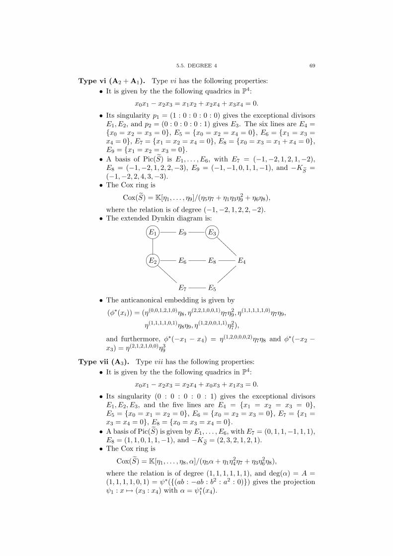
5.5. DEGREE 4 69
Type vi (A2 + A1). Type vi has the following properties:• It is given by the the following quadrics in P4:
x0x1 − x2x3 = x1x2 + x2x4 + x3x4 = 0.
• Its singularity p1 = (1 : 0 : 0 : 0 : 0) gives the exceptional divisorsE1, E2, and p2 = (0 : 0 : 0 : 0 : 1) gives E3. The six lines are E4 ={x0 = x2 = x3 = 0}, E5 = {x0 = x2 = x4 = 0}, E6 = {x1 = x3 =x4 = 0}, E7 = {x1 = x2 = x4 = 0}, E8 = {x0 = x3 = x1 + x4 = 0},E9 = {x1 = x2 = x3 = 0}.
• A basis of Pic(S) is E1, . . . , E6, with E7 = (−1,−2, 1, 2, 1,−2),E8 = (−1,−2, 1, 2, 2,−3), E9 = (−1,−1, 0, 1, 1,−1), and −KeS =(−1,−2, 2, 4, 3,−3).
• The Cox ring is
Cox(S) = K[η1, . . . , η9]/(η5η7 + η1η3η29 + η6η8),
where the relation is of degree (−1,−2, 1, 2, 2,−2).• The extended Dynkin diagram is:
GFED@ABCE1 E9GFED@ABCE3
@@@@
@@@@
@
GFED@ABCE2
BBBB
BBBB
E6 E8 E4
E7 E5
||||||||
• The anticanonical embedding is given by
(φ∗(xi)) = (η(0,0,1,2,1,0)η8, η(2,2,1,0,0,1)η7η
29, η
(1,1,1,1,1,0)η7η9,
η(1,1,1,1,0,1)η8η9, η(1,2,0,0,1,1)η2
7),
and furthermore, φ∗(−x1 − x4) = η(1,2,0,0,0,2)η7η8 and φ∗(−x2 −x3) = η(2,1,2,1,0,0)η3
9
Type vii (A3). Type vii has the following properties:• It is given by the the following quadrics in P4:
x0x1 − x2x3 = x2x4 + x0x3 + x1x3 = 0.
• Its singularity (0 : 0 : 0 : 0 : 1) gives the exceptional divisorsE1, E2, E3, and the five lines are E4 = {x1 = x2 = x3 = 0},E5 = {x0 = x1 = x2 = 0}, E6 = {x0 = x2 = x3 = 0}, E7 = {x1 =x3 = x4 = 0}, E8 = {x0 = x3 = x4 = 0}.
• A basis of Pic(S) is given by E1, . . . , E6, with E7 = (0, 1, 1,−1, 1, 1),E8 = (1, 1, 0, 1, 1,−1), and −KeS = (2, 3, 2, 1, 2, 1).
• The Cox ring is
Cox(S) = K[η1, . . . , η8, α]/(η5α+ η1η24η7 + η3η
26η8),
where the relation is of degree (1, 1, 1, 1, 1, 1), and deg(α) = A =(1, 1, 1, 1, 0, 1) = ψ∗({(ab : −ab : b2 : a2 : 0)}) gives the projectionψ1 : x 7→ (x3 : x4) with α = ψ∗1(x4).

70 5. UNIVERSAL TORSORS WHICH ARE HYPERSURFACES
• The extended Dynkin diagram is:
E7
????
????
? E4GFED@ABCE1
BBBB
BBBB
B
A E5GFED@ABCE2
E8
���������E6
GFED@ABCE3
|||||||||
Here, A,E7, E8 meet in (0 : 0 : 1 : 0 : 0).• The anticanonical embedding is given by
(φ∗(xi)) = (η(2,2,1,2,1,0)η7, η(1,2,2,0,1,2)η8, η
(2,3,2,1,2,1), η(1,1,1,1,0,1)η7η8, η7η8α),
and furthermore, φ∗(−x0 − x1) = η(1,2,1,0,2,0)α
Type xi (A3 + A1). Type xi has the following properties:• It is given by the the following quadrics in P4:
x0x3 − x2x4 = x0x1 + x1x3 + x22 = 0.
• The singularity p1 = (0 : 1 : 0 : 0 : 0) gives an exceptional divisorE1, and p2 = (0 : 0 : 0 : 0 : 1) gives E2, E3, E4. The three linesare E5 = {x0 = x2 = x3 = 0}, E6 = {x0 = x1 = x2 = 0},E7 = {x1 = x2 = x3 = 0}.
• A basis of Pic(S) is E1, . . . , E6, with E7 = (1,−1, 0, 1, 2,−1) and−KeS = (2, 1, 2, 3, 4, 0).
• The Cox ring is
Cox(S) = K[η1, . . . , η7, α1, α2]/(η6α2 + η7α1 + η1η3η24η
35),
where the relation is of degree (1, 0, 1, 2, 3, 0), deg(α1) = A1 =(0, 1, 1, 1, 1, 1) = ψ∗({(a2 : −b2 : ab : 0 : 0)}) gives the projec-tion ψ1 : x 7→ (x2 : x3) with α1 = ψ∗1(x3), and deg(α2) = A2 =(1, 0, 1, 2, 3,−1) = ψ∗({(0 : a2 : ab : −b2 : 0)}) gives the projectionψ2 : x 7→ (x0 : x2) with α2 = ψ∗2(x0).
• The extended Dynkin diagram is:
A1
BBBB
BBBB
E7
CCCC
CCCC
C
GFED@ABCE1 E5GFED@ABCE4
GFED@ABCE3GFED@ABCE2
A2
||||||||E6
{{{{{{{{{
Here, A1, A2, E1 meet in one point.• The anticanonical embedding is given by
(φ∗(xi)) = (η(1,1,1,1,1,1)α2, η(0,3,2,1,0,2)η2
7, η(1,2,2,2,2,1)η7,
η(1,1,1,1,1,0)η7α1, η(1,0,0,0,0,0)α1α2),
and furthermore, φ∗(−x0 − x3) = η(2,1,2,3,4,0).

5.5. DEGREE 4 71
Type xii (A4). Type xii has the following properties:• It is given by the the following quadrics in P4:
x0x1 − x2x3 = x0x4 + x1x2 + x23 = 0.
• The singularity p = (0 : 0 : 0 : 0 : 1) gives the exceptional divisorsE1, . . . , E4, and the three lines are E5 = {x0 = x2 = x3 = 0},E6 = {x0 = x1 = x3 = 0}, and E7 = {x1 = x3 = x4 = 0}.
• A basis of Pic(S) is given by E1, . . . , E6, with E7 = (1, 2, 1, 0, 2,−1),and −KeS = (2, 4, 3, 2, 3, 1).
• The Cox ring is
Cox(S) = K[η1, . . . , η7, α1, α2]/(η5α1 + η1α22 + η3η
24η
36η7),
where the degree of the relation is (1, 2, 2, 2, 2, 2), and deg(α1) =A1 = (1, 2, 2, 2, 1, 2) = ψ∗({(−b3 : a3 : −ab2 : a2b : 0)}) gives theprojection ψ1 from E7, with α1 = ψ∗1(x4), and deg(α2) = A2 =(0, 1, 1, 1, 1, 1) = ψ∗({(a2 : 0 : 0 : −ab : b2)}) gives the projectionψ2 : x 7→ (x1 : x3) with α2 = ψ∗2(x1).
• The extended Dynkin diagram is:
A1
AAAA
AAAA
E5
CCCC
CCCC
C
E7 E6GFED@ABCE4
GFED@ABCE3GFED@ABCE2
||||
||||
|
A2
�������� GFED@ABCE1
Here, A1, A2, E7 meet in (1 : 0 : 0 : 0 : 0).• The anticanonical embedding is given by
(φ∗(xi)) = (η(2,4,3,2,3,1), η(1,1,1,1,0,1)η7α2, η(2,3,2,1,2,0)α2, η
(1,2,2,2,1,2)η7, η7α1).
Type xiii (D4). Type xiii, which is considered in more detail in Chapter 10(see [BB05] for a form whose lines are not defined over Q), has the followingproperties:
• It is given by the the following quadrics in P4:
x0x3 − x1x4 = x0x1 + x1x3 + x22 = 0.
• The singularity p = (0 : 0 : 0 : 0 : 1) gives four exceptional divisorE1, . . . , E4, and its lines are E5 = {x0 = x1 = x2 = 0} and E6 ={x1 = x2 = x3 = 0}.
• A basis of Pic(S) is given by E1, . . . , E6, and −KeS = (4, 2, 3, 3, 2, 2).• The Cox ring is
Cox(S) = K[η1, . . . , η6, α1, α2, α3]/(η3η25α2 + η4η
26α3 + η2α
21),
where the degree of the relation is (2, 1, 2, 2, 2, 2), deg(α1) = A1 =(1, 0, 1, 1, 1, 1) = ψ∗({(ab : b2 : 0 : −ab : −a2)}) gives the pro-jection ψ1 : x 7→ (x1 : x2) with α1 = ψ∗1(x2), deg(α2) = A2 =(2, 1, 1, 2, 0, 2) = ψ∗({(0 : a2 : ab : −b2 : 0)}) gives the projec-tion ψ2 : x 7→ (x0 : x1) with α2 = ψ∗2(x0), and deg(α3) = A3 =

72 5. UNIVERSAL TORSORS WHICH ARE HYPERSURFACES
(2, 1, 2, 1, 2, 0) = ψ∗({(a2 : −b2 : ab : 0 : 0)}) gives the projectionψ3 : x 7→ (x1 : x3) with α3 = ψ∗3(x3).
• The extended Dynkin diagram is:
A2
????
????
E5GFED@ABCE3
BBBB
BBBB
B
A1GFED@ABCE2
GFED@ABCE1
A3
��������E6
GFED@ABCE4
|||||||||
Here, A1, A2, A3 intersect in (0 : 1 : 0 : 0 : 0).• The anticanonical embedding is given by
(φ∗(xi)) = (η(2,1,2,1,2,0)α2, η(4,2,3,3,2,2), η(3,2,2,2,1,1)α1, η
(2,1,1,2,0,2)α3, α2α3).
Furthermore, φ∗(−x0 − x3) = η(2,2,1,1,0,0)α21.
Type xv (D5). Type xv, which has already been considered in [BB04],has the following properties:
• It is given by the the following quadrics in P4:
x0x1 − x22 = x2
3 + x0x4 + x1x2 = 0
• The singularity p = (0 : 0 : 0 : 0 : 1) gives five exceptional divisorE1, . . . , E5, and its line is E6 = {x0 = x2 = x3 = 0}.
• A basis of Pic(S) is given by E1, . . . , E6, and −KeS = (6, 5, 3, 4, 2, 4).• The Cox ring is
Cox(S) = K[η1, . . . , η6, α1, α2, α3]/(η3α21 + η2η
26α3 + η4η
25α
32),
where the degree of the relation is (6, 6, 3, 4, 2, 6), and deg(α1) =A1 = (3, 3, 1, 2, 1, 3) = ψ∗({(a3 : ab2 : a2b : 0 : −a3)}) givesthe projection ψ1 from E6 with α1 = ψ∗1(x3), deg(α2) = A2 =(2, 2, 1, 1, 0, 2) = ψ∗({(a2 : 0 : 0 : ab : −b2)}) gives the projec-tion ψ2 : x 7→ (x0 : x2) with α2 = ψ∗2(x2), and deg(α3) = A3 =−KeS = ψ∗({(−a4 : −b4 : a2b2 : ab3 : 0)}) gives the anticanonicalembedding φ with α3 = φ∗(x4).
• The extended Dynkin diagram is:
A2
@@@@
@@@@
@GFED@ABCE5
GFED@ABCE4
BBBB
BBBB
B
A1GFED@ABCE3
GFED@ABCE1
A3
~~~~~~~~~E6
GFED@ABCE2
|||||||||
where A1, A2, A3 intersect in (1 : 0 : 0 : 0 : 0).• For the anticanonical embedding,
(φ∗(xi)) = (η(6,5,3,4,2,4), η(2,1,1,2,2,0)α22, η
(4,3,2,3,2,2)α2, η(3,2,2,2,1,1)α1, α3).
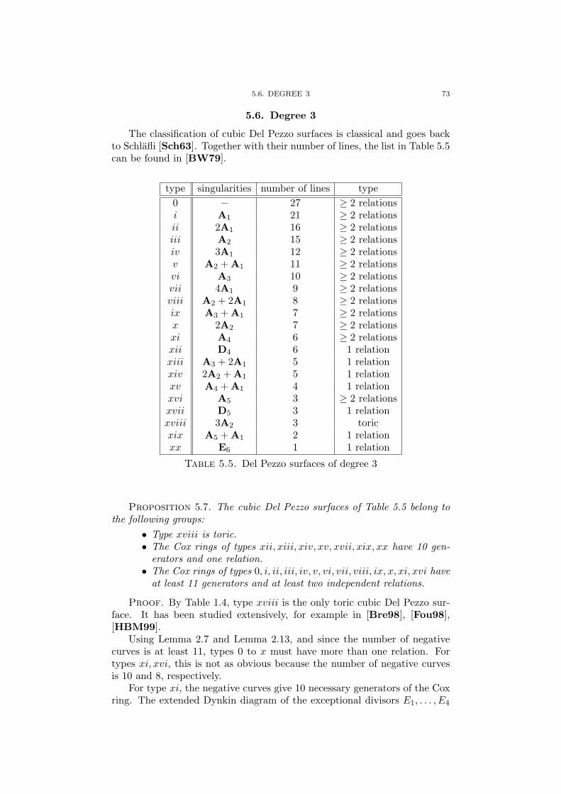
5.6. DEGREE 3 73
5.6. Degree 3
The classification of cubic Del Pezzo surfaces is classical and goes backto Schlafli [Sch63]. Together with their number of lines, the list in Table 5.5can be found in [BW79].
type singularities number of lines type0 − 27 ≥ 2 relationsi A1 21 ≥ 2 relationsii 2A1 16 ≥ 2 relationsiii A2 15 ≥ 2 relationsiv 3A1 12 ≥ 2 relationsv A2 + A1 11 ≥ 2 relationsvi A3 10 ≥ 2 relationsvii 4A1 9 ≥ 2 relationsviii A2 + 2A1 8 ≥ 2 relationsix A3 + A1 7 ≥ 2 relationsx 2A2 7 ≥ 2 relationsxi A4 6 ≥ 2 relationsxii D4 6 1 relationxiii A3 + 2A1 5 1 relationxiv 2A2 + A1 5 1 relationxv A4 + A1 4 1 relationxvi A5 3 ≥ 2 relationsxvii D5 3 1 relationxviii 3A2 3 toricxix A5 + A1 2 1 relationxx E6 1 1 relation
Table 5.5. Del Pezzo surfaces of degree 3
Proposition 5.7. The cubic Del Pezzo surfaces of Table 5.5 belong tothe following groups:
• Type xviii is toric.• The Cox rings of types xii, xiii, xiv, xv, xvii, xix, xx have 10 gen-
erators and one relation.• The Cox rings of types 0, i, ii, iii, iv, v, vi, vii, viii, ix, x, xi, xvi have
at least 11 generators and at least two independent relations.
Proof. By Table 1.4, type xviii is the only toric cubic Del Pezzo sur-face. It has been studied extensively, for example in [Bre98], [Fou98],[HBM99].
Using Lemma 2.7 and Lemma 2.13, and since the number of negativecurves is at least 11, types 0 to x must have more than one relation. Fortypes xi, xvi, this is not as obvious because the number of negative curvesis 10 and 8, respectively.
For type xi, the negative curves give 10 necessary generators of the Coxring. The extended Dynkin diagram of the exceptional divisors E1, . . . , E4

74 5. UNIVERSAL TORSORS WHICH ARE HYPERSURFACES
and the six lines E5, . . . , E10 is:
E5GFED@ABCE2
GFED@ABCE3GFED@ABCE4
GFED@ABCE1
|||||||||E9 E7
|||||||||E8
E6
{{{{{{{{E10
{{{{{{{{
A basis of Pic(S) is given by E1, . . . , E7, and in terms of this basis,
E8 = (1, 1, 0,−1, 1, 1,−1), E9 = (1, 2, 1, 0, 2, 0,−1),
E10 = (0, 1, 1, 1, 1,−1, 1), −KeS = (2, 3, 2, 1, 2, 1, 0).
The divisors E1, . . . , E10 generate the effective cone. We check that A =(1, 1, 1, 1, 0, 1, 1) is nef. Therefore, we calculate dimH0(A) = χ(A) = 2by Riemann-Roch. However, the subring generated by non-zero sections ofH0(Ei) does not give two linearly independent sections in H0(A). Hence,Cox(S) must have more than 10 generators.
For type xvi, we have the following information:• The singularity gives the exceptional divisors E1, . . . , E5, and there
are three lines E6, E7, E8.• The extended Dynkin diagram of negative curves is:
GFED@ABCE1GFED@ABCE2
GFED@ABCE3GFED@ABCE4
GFED@ABCE5 E6
E7 E8
• A basis of Pic(S) is E1, . . . , E7, with E8 = (1, 2, 1, 0,−1,−1, 2) and−KeS = (2, 4, 3, 2, 1, 0, 3).
• Three of the 13 generators of the nef cone are B1 = (0, 1, 1, 1, 1, 1),B2 = (1, 3, 2, 1, 0,−1, 3), B3 = (1, 2, 2, 2, 2, 2, 1), with
dim(H0(B1)) = dim(H0(B2)) = 2, dim(H0(B3)) = 3.
As for type viii of degree 4, we check that a minimal system of generatorsof Cox(S) can be assumed to contain η1, . . . , η8 with non-zero ηj ∈ H0(Ej),and β1, β2 of degree B1, B2, respectively. However, it is not hard to checkthat the subring of Cox(S) generated by η1, . . . , η8, β1, β2 contains only twolinearly independent sections in degree B3. Therefore, Cox(S) must havemore than 10 generators.
For each type whose Cox ring has exactly 10 generators, the calculationsfollow below. �
Remark 5.8. By [BW79], some types of cubic surfaces do not have asingle normal form, but a family with one or more parameters. More pre-cisely, this happens exactly for the types 0, i, ii, iii, iv, v, vi, x. Furthermore,by [BW79, Lemma 4], the D4 cubic surface (type xii) is the only surfacewhich has more than one normal form, but not a family. The two differentsurfaces with a D4 singularity are also discussed in [HT04, Remark 4.1].

5.6. DEGREE 3 75
Type xii (D4). As mentioned above, type xii has two different forms:• The first is given by
x0(x1 + x2 + x3)2 − x1x2x3 = 0,
the second by
x0(x1 + x2 + x3)2 + x1x2(x1 + x2) = 0.
• The singularity is p = (1 : 0 : 0 : 0), giving four exceptional divisorsE1, . . . , E4. In the first form, the six lines are E5 = {x1 = x2 +x3 = 0}, E6 = {x2 = x1 + x3 = 0}, E7 = {x3 = x1 + x2 = 0},E8 = {x0 = x1 = 0}, E9 = {x0 = x2 = 0}, E10 = {x0 = x3 = 0}.In the second form, E10 is replaced by {x0 = x1 + x2 = 0}.
• A basis of Pic(S) is given by E1, . . . , E7, with
E8 = (1, 0, 1, 1,−1, 1, 1), E9 = (1, 1, 0, 1, 1,−1, 1),
E10 = (1, 1, 1, 0, 1, 1,−1), −KeS = (3, 2, 2, 2, 1, 1, 1).
• The Cox ring is
Cox(S) = K[η1, . . . , η10]/(η2η25η8 + η3η
26η9 + η4η
27η10 −A · η1η2η3η4η5η6η7),
where the constant A is 1 for the first form and 0 for the secondform, and the degree of the relation is (1, 1, 1, 1, 1, 1, 1).
• The extended Dynkin diagram is:
GFED@ABCE2 E5 E8
}}}}
}}}}
GFED@ABCE1GFED@ABCE2 E6 E9
AAAA
AAAA
GFED@ABCE4 E7 E10
The lines E8, E9, E10 meet in one point only in case of the secondform.
• For the first form, the anticanonical embedding φ : S → P3 is givenby
(φ∗(xi)) = (η8η9η10, η(2,2,1,1,2,0,0)η8, η
(2,1,2,1,0,2,0)η9, η(2,1,1,2,0,0,2)η10),
and furthermore, φ∗(x1 +x2 +x3) = η(3,2,2,2,1,1,1). The second formdiffers from this as follows: φ∗(−x1 − x2) = η(2,1,1,2,0,0,2)η10, andφ∗(x3) = η(3,2,2,2,1,1,1) + η(2,1,1,2,0,0,2)η10.
Type xiii (A3 + 2A1). Type xiii has the following properties:• It is given by the following cubic in P3:
x23(x1 + x2) + x0x1x2 = 0.
• The singularities in p1 = (0 : 1 : 0 : 0) and p2 = (0 : 0 : 1 : 0)give exceptional divisors E1, E10, respectively, and the singularityin p3 = (1 : 0 : 0 : 0) gives E2, E3, E4. The five lines are given byE5 = {x0 = x3 = 0}, E6 = {x1 = x3 = 0}, E7 = {x2 = x3 = 0},E8 = {x1 = x2 = 0}, E9 = {x0 = x1 + x2 = 0}.

76 5. UNIVERSAL TORSORS WHICH ARE HYPERSURFACES
• A basis of the Pic(S) is E1, . . . , E7, and E8 = (1, 0,−1,−1, 1,−1, 1),E9 = (0, 1, 1, 1,−1, 1, 1), E10 = (1, 1, 0,−1, 0,−2, 2), and −KeS =(2, 2, 1, 0, 1,−1, 3).
• The Cox ring is
Cox(S) = K[η1, . . . , η10]/(η4η26η10 + η1η2η
27 + η8η9),
where the relation is of degree (1, 1, 0, 0, 0, 0, 2).• The extended Dynkin diagram is:
GFED@ABCE2 E7GFED@ABCE1
BBBB
BBBB
B
GFED@ABCE3 E8 E9 E5
GFED@ABCE4 E6GFED@ABCE10
|||||||||
• For the anticanonical embedding,
(φ∗(xi)) = (η(1,0,0,0,2,0,0)η9η10, η(0,1,2,2,0,2,0)η8η10,
η(1,2,2,1,0,0,2)η8, η(1,1,1,1,1,1,1)η10),
and furthermore, φ∗(−x1 − x2) = η(0,1,2,1,0,0,0)η28η9.
Type xiv (2A2 + A1). Type xiv has the following properties:• Its equation is
x23(x1 + x3) + x0x1x2 = 0.
• The singularity (0 : 1 : 0 : 0) gives an exceptional divisor E1, and(1 : 0 : 0 : 0) gives E2, E3, and (0 : 0 : 1 : 0) gives E4, E5. The linesare E6 = {x0 = x3 = 0}, E7 = {x1 = x3 = 0}, E8 = {x2 = x3 = 0},E9 = {x0 = x1 + x3 = 0}, E10 = {x2 = x1 + x3 = 0}.
• A basis of Pic(S) is E1, . . . , E7, and E8 = (−1, 0, 1, 0, 1,−1, 2), E9 =(−1, 1, 2,−1, 1,−2, 3), E10 = (1,−1,−1, 1, 0, 2,−1), and −KeS =(0, 1, 2, 1, 2, 0, 3).
• The Cox ring is
Cox(S) = K[η1, . . . , η10]/(η3η5η27 + η1η6η8 + η9η10),
where the relation is of degree (0, 0, 1, 0, 1, 0, 2).• The extended Dynkin diagram is:
E8GFED@ABCE1 E6
BBBB
BBBB
B
GFED@ABCE2
|||||||||
CCCC
CCCC
CGFED@ABCE3 E7
GFED@ABCE5GFED@ABCE4
E10 E9
{{{{{{{{{

5.6. DEGREE 3 77
• For the anticanonical embedding,
(φ∗(xi)) = (η(1,0,0,2,1,2,0)η9, η(0,1,2,1,2,0,3), η(1,2,1,0,0,0,0)η2
8η10, η(1,1,1,1,1,1,1)η8),
and furthermore, φ∗(−x1 − x3) = η(0,1,1,1,1,0,1)η9η10.
Type xv (A4 + A1). Type xv has the following properties:• Its equation is
x2x23 + x2
1x3 + x0x1x2 = 0.
• The singularity (0 : 0 : 1 : 0) gives an exceptional divisor E9, and(1 : 0 : 0 : 0) gives E1, . . . , E4. The lines are E5 = {x0 = x3 = 0},E6 = {x1 = x3 = 0}, E7 = {x1 = x2 = 0}, E8 = {x2 = x3 = 0}.
• A basis of Pic(S) is E1, . . . , E7, and E8 = (0, 1, 1, 1,−1, 1, 1), E9 =(1, 2, 1, 0,−1,−1, 2), and −KeS = (2, 4, 3, 2,−1, 1, 3).
• The Cox ring is
Cox(S) = K[η1, . . . , η9, α]/(η1η5η28 + η3η
24η
36η9 + η7α),
where the relation is of degree (1, 2, 2, 2,−1, 2, 2), and deg(α) =A = (1, 2, 2, 2,−1, 2, 1) = ψ∗({(0 : ab : a2 : −b2)}) describes theprojection ψ1 from E5, with α = ψ∗1(x0).
• The extended Dynkin diagram is:
GFED@ABCE9
@@@@
@@@@
@ E6GFED@ABCE4
GFED@ABCE3
BBBB
BBBB
B
E5 E8GFED@ABCE1
GFED@ABCE2
A
||||||||E7
{{{{{{{{{
Here, A,E5, E9 meet in one point.• The anticanonical embedding is given by
(φ∗(xi)) = (η5η9α, η(1,2,2,2,0,2,1)η9, η
(2,3,2,1,0,0,2)η8, η(1,1,1,1,1,1,0)η8η9).
Type xvii (D5). Type xvii has the following properties:• Its equation is
x3x20 + x0x
22 + x2
1x2 = 0.
• The singularity (0 : 0 : 0 : 1) gives exceptional divisors E1, . . . , E5.The lines are E6 = {x0 = x1 = 0}, E7 = {x0 = x2 = 0}, andE8 = {x2 = x3 = 0}.
• A basis of Pic(S) is E1, . . . , E7, with E8 = (2, 2, 1, 1, 0, 2,−1) and−KeS = (4, 3, 2, 3, 2, 2, 1).
• The Cox ring is
Cox(S) = K[η1, . . . , η8, α1, α2]/(η2η26α2 + η4η
25η
37η8 + η3α
21),
where the relation has degree (2, 2, 1, 2, 2, 2, 2), and deg(α1) = A1 =(1, 1, 0, 1, 1, 1, 1) = ψ∗({(a2 : 0 : ab : −b2)}) describes a projectionψ1 from E6 with α1 = ψ∗1(x1), deg(α2) = A2 = (2, 1, 1, 2, 2, 0, 2) =
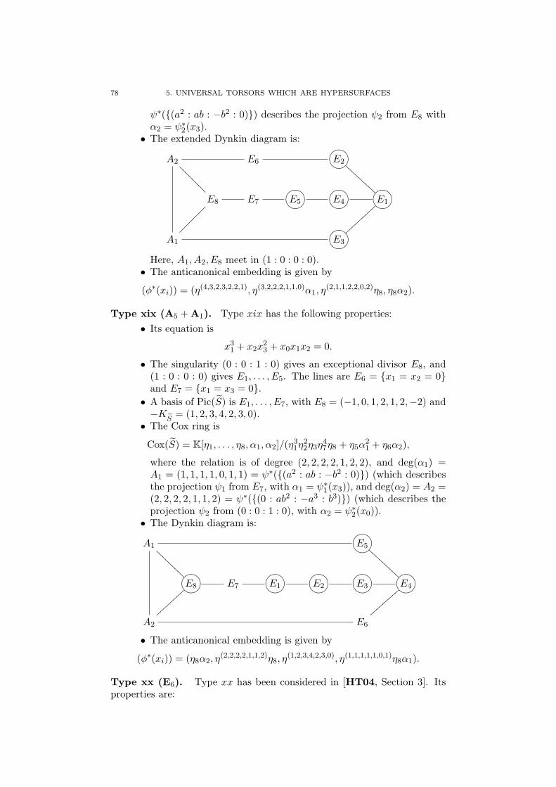
78 5. UNIVERSAL TORSORS WHICH ARE HYPERSURFACES
ψ∗({(a2 : ab : −b2 : 0)}) describes the projection ψ2 from E8 withα2 = ψ∗2(x3).
• The extended Dynkin diagram is:
A2
????
????
E6GFED@ABCE2
BBBB
BBBB
B
E8 E7GFED@ABCE5
GFED@ABCE4GFED@ABCE1
A1
�������� GFED@ABCE3
|||||||||
Here, A1, A2, E8 meet in (1 : 0 : 0 : 0).• The anticanonical embedding is given by
(φ∗(xi)) = (η(4,3,2,3,2,2,1), η(3,2,2,2,1,1,0)α1, η(2,1,1,2,2,0,2)η8, η8α2).
Type xix (A5 + A1). Type xix has the following properties:• Its equation is
x31 + x2x
23 + x0x1x2 = 0.
• The singularity (0 : 0 : 1 : 0) gives an exceptional divisor E8, and(1 : 0 : 0 : 0) gives E1, . . . , E5. The lines are E6 = {x1 = x2 = 0}and E7 = {x1 = x3 = 0}.
• A basis of Pic(S) is E1, . . . , E7, with E8 = (−1, 0, 1, 2, 1, 2,−2) and−KeS = (1, 2, 3, 4, 2, 3, 0).
• The Cox ring is
Cox(S) = K[η1, . . . , η8, α1, α2]/(η31η
22η3η
47η8 + η5α
21 + η6α2),
where the relation is of degree (2, 2, 2, 2, 1, 2, 2), and deg(α1) =A1 = (1, 1, 1, 1, 0, 1, 1) = ψ∗({(a2 : ab : −b2 : 0)}) (which describesthe projection ψ1 from E7, with α1 = ψ∗1(x3)), and deg(α2) = A2 =(2, 2, 2, 2, 1, 1, 2) = ψ∗({(0 : ab2 : −a3 : b3)}) (which describes theprojection ψ2 from (0 : 0 : 1 : 0), with α2 = ψ∗2(x0)).
• The Dynkin diagram is:
A1
@@@@
@@@@
@GFED@ABCE5
BBBB
BBBB
B
GFED@ABCE8 E7GFED@ABCE1
GFED@ABCE2GFED@ABCE3
GFED@ABCE4
A2
||||||||E6
{{{{{{{{{
• The anticanonical embedding is given by
(φ∗(xi)) = (η8α2, η(2,2,2,2,1,1,2)η8, η
(1,2,3,4,2,3,0), η(1,1,1,1,1,0,1)η8α1).
Type xx (E6). Type xx has been considered in [HT04, Section 3]. Itsproperties are:
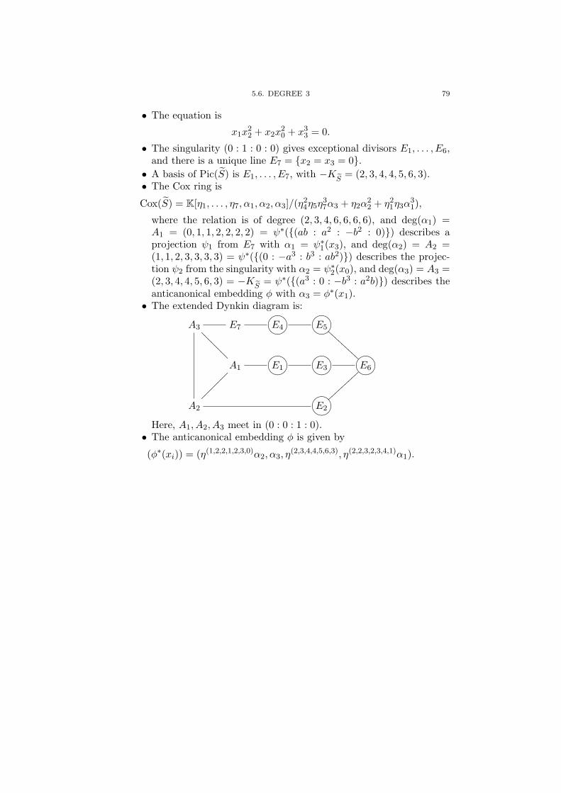
5.6. DEGREE 3 79
• The equation is
x1x22 + x2x
20 + x3
3 = 0.
• The singularity (0 : 1 : 0 : 0) gives exceptional divisors E1, . . . , E6,and there is a unique line E7 = {x2 = x3 = 0}.
• A basis of Pic(S) is E1, . . . , E7, with −KeS = (2, 3, 4, 4, 5, 6, 3).• The Cox ring is
Cox(S) = K[η1, . . . , η7, α1, α2, α3]/(η24η5η
37α3 + η2α
22 + η2
1η3α31),
where the relation is of degree (2, 3, 4, 6, 6, 6, 6), and deg(α1) =A1 = (0, 1, 1, 2, 2, 2, 2) = ψ∗({(ab : a2 : −b2 : 0)}) describes aprojection ψ1 from E7 with α1 = ψ∗1(x3), and deg(α2) = A2 =(1, 1, 2, 3, 3, 3, 3) = ψ∗({(0 : −a3 : b3 : ab2)}) describes the projec-tion ψ2 from the singularity with α2 = ψ∗2(x0), and deg(α3) = A3 =(2, 3, 4, 4, 5, 6, 3) = −KeS = ψ∗({(a3 : 0 : −b3 : a2b)}) describes theanticanonical embedding φ with α3 = φ∗(x1).
• The extended Dynkin diagram is:
A3
????
????
E7GFED@ABCE4
GFED@ABCE5
BBBB
BBBB
B
A1GFED@ABCE1
GFED@ABCE3GFED@ABCE6
A2
�������� GFED@ABCE2
|||||||||
Here, A1, A2, A3 meet in (0 : 0 : 1 : 0).• The anticanonical embedding φ is given by
(φ∗(xi)) = (η(1,2,2,1,2,3,0)α2, α3, η(2,3,4,4,5,6,3), η(2,2,3,2,3,4,1)α1).


CHAPTER 6
Cox rings of generalized Del Pezzo surfaces
6.1. Introduction
Let Sr be the blow-up of P2 in r ≤ 8 points in almost general positionover an algebraically closed field K, i.e., a generalized Del Pezzo surface ofdegree 9− r (Section 1.5). We restrict ourselves to the case r ≤ 7.
If Sr is a smooth Del Pezzo surface, the Cox ring is known explicitly(see Chapter 3). For generalized Del Pezzo surfaces, the Cox ring can bedetermined for toric Sr by results of Cox (see Lemma 2.12), and in cases withexactly one relation in the Cox ring by a method of Hassett and Tschinkel(see Chapter 5).
The purpose of this chapter is to show how generators and relations (upto radical) of Cox(Sr) can be determined explicitly for any generalized DelPezzo surface, in particular including Cox rings with more than one relation.
Compared to the case of non-toric smooth Del Pezzo surfaces, this prob-lem has several complications:
• While there is only one type of smooth Del Pezzo surfaces in eachdegree, there are, for example, 20 more types of generalized cubicDel Pezzo surface.
• In the smooth case, every generator of the Cox ring corresponds to anegative curve. For generalized Del Pezzo surfaces, extra generatorscan occur (see Chapter 5 for examples).
• The Weyl group symmetry of the configuration of (−1)-curves onsmooth Del Pezzo surfaces (Section 1.4) can be used when deter-mining the Cox ring. The configuration of negative curves (includ-ing (−2)-curves) on generalized Del Pezzo surfaces is usually lesssymmetric.
However, we will refine arguments of [BP04] in Section 6.2 to describegenerators of Cox(Sr). Every generator corresponds to a negative curve onSr, or has degree −KeSr
, or is the pull-back of a generator of Cox(Sr−1),
where Sr−1 is obtained by the contraction of a (−1)-curve on Sr.Having determined Nr generators of Cox(Sr), we may think of Cox(Sr)
in terms of the affine variety A(Sr) = Spec(Cox(Sr)) embedded in ANr .Determining the ideal of relations in Cox(Sr) up to radical is equivalent tofinding equations defining A(Sr).
The ideas of [HT04] help to find certain relations in Cox(Sr) even whenthere is more than one relation. However, the proof of [HT04] that thesingle relation defines Cox(Sr) does not generalize to a situation where morerelations occur.
81

82 6. COX RINGS OF GENERALIZED DEL PEZZO SURFACES
Instead, we proceed as follows. Let E be a (−1)-curve on Sr. Let UE bethe open subset of AN where the coordinate corresponding to E does notvanish. By Lemma 1.35, contracting E results in a generalized Del Pezzosurface Sr−1. We will see that
A(Sr) ∩ UE∼= A(Sr−1)× (A1 \ {0}).
This will allow us to determine A(Sr) ∩ UE recursively, and since A(Sr)is irreducible, we obtain the ideal of relations up to radical by taking theclosure. See Section 6.3 for more details.
In a series of examples of quartic and cubic Del Pezzo surfaces, we willsee that the methods to determine the generators and relations in Cox(Sr),as described in Sections 6.2 and 6.3, can be made explicit in practice. As ourapproach relates Cox(Sr) to the case r − 1, we apply the results for degree5 (where the Cox ring of every singular surface has at most one relation) ofSection 5.4 and degree 4 of Section 5.5 whenever the surface Sr−1 obtainedfrom Sr by contracting a (−1)-curve has a Cox ring with exactly one relation.
In the examples, we use notation from previous chapters, in particularChapter 5.
6.2. Generators
In this section, we show how to determine generators of Cox(Sr), whereSr is the minimal desingularization of a singular Del Pezzo surface Sr ofdegree 9− r ≥ 2.
Lemma 6.1. For 2 ≤ r ≤ 7, let Sr be a generalized Del Pezzo surface ofdegree 9 − r. Let D ∈ Pic(Sr) such that (D,E) ≥ 0 for all negative curvesE on Sr. Then the linear system |D| has no base points.
Proof. We use induction on r, starting with the case r = 2. Thesurface S2 of degree 7 can be a smooth Del Pezzo surface or a generalizedDel Pezzo surface of type A1 which is obtained from P2 by blowing up onepoint and another point on the exceptional divisor of the first blow-up. Thesmooth case is covered by [BP04, Proposition 2.3]. In the second case,we have (in terms of the standard basis as in Lemma 1.7) the (−2)-curveE1 = l1 − l2 and the (−1)-curves E2 = l2 and E3 = l0 − l1 − l2. Thenegative curves E1, E2, E3 are also a basis of Pic(S2). The dual basiswith respect to the intersection form consists of l0 − l1 (defining a conicbundle fibration S2 → P1), 2l0 − l1 − l2 (defining a morphism S2 → P3),and l0 (defining S2 → P2), so the corresponding linear systems have no basepoints. A general D is a non-negative integral linear combination of thesethree elements, and, therefore, |D| also has no base points.
For r ≥ 3, if there is a (−1)-curve E ⊂ Sr with (D,E) = 0, thenwe consider the map πE : Sr → Sr−1 which contracts E, where Sr−1 is ageneralized Del Pezzo surface of degree 9−(r−1). We haveO(D) = π∗EO(D′)for some invertible sheaf O(D′) on Sr−1. As the negative curves of Sr−1 areimages of negative curves of Sr under πE , the divisor D′ is nef. By inductionon r, the linear system |D′| has no base points. Consequently, |D| = |π∗ED′|has no base points.

6.2. GENERATORS 83
If there is no (−1)-curve E ⊂ Sr with (D,E) = 0, then let m > 0 be theminimal number (D,E) for all (−1)-curves E. Since (E,−KeSr
) = 1 for all(−1)-curves and (E,−KeSr
) = 0 for all (−2)-curves, D′ := D −m · (−KeSr)
is nef, and (D′, E) = 0 for some (−1)-curve E. As discussed before, |D′|has no base points. Since r ≤ 7, the system | −KeSr
| is also base point free.Therefore, |D| has no base points. �
For r = 2, the Del Pezzo surfaces S2 of degree 7 are toric. Hence,generators of Cox(S2) are known (Lemma 2.12). For larger r, they can bedetermined recursively as follows. Suppose that we can find a finite setof generators of Cox(Sr−1) for any generalized Del Pezzo surface of degree9− (r − 1).
For every (−1)-curve E on Sr, let πE : Sr → Sr−1 be the contraction of Eresulting in a generalized Del Pezzo surface Sr−1, and choose a homogeneoussystem of generators of Cox(Sr−1).
An element of Cox(Sr) is called a distinguished section if it is one of thefollowing:
• A section ξ(E) corresponding to a negative curve E on Sr (cf.Lemma 1.3).
• A global section of −KeSr.
• A section π∗E(α), where πE : Sr → Sr−1 is as above, and the sectionα is an element of the chosen homogeneous system of generators ofCox(Sr−1) which does not vanish in πE(E) and does not correspondto a negative curve on Sr−1.
Theorem 6.2. For 3 ≤ r ≤ 7, the Cox ring Cox(Sr) is generated bya finite set of distinguished sections which can be determined explicitly, in-cluding at most two global sections of −KeSr
.
Proof. Let k(D) be the number of fixed components of D which are(−2)-curves of Sr. If k(D) > 0 and the (−2)-curve E is a fixed componentof D, then k(D − E) = k(D) − 1. If k(D) = 0, then (D,E) ≥ 0 for any(−2)-curve E since E is the only prime divisor which intersects E negatively.
For each effective divisor D on Sr, we want to show that H0(Sr,O(D))is generated by the distinguished sections. We use induction over deg(D) :=(D,−KeSr
). Note that D is not effective if deg(D) < 0. In each degree, weuse a second induction over k(D).
(1) If there exists a negative curve E with (D,E) < 0, then E is a fixedcomponent of D. The sequence
H0(Sr,O(D − E)) → H0(Sr,O(D)) → H0(E,O(D)|E)
is exact, where the first map is multiplication with ξ(E). SinceH0(E,O(D)|E) = 0, the claim follows from the induction assump-tion for D − E, where k(D − E) < k(D) if E is a (−2)-curve, anddeg(D − E) < deg(D) if E is a (−1)-curve.
(2) If there exists a (−1)-curve E with (D,E) = 0, consider the mapπE : Sr → Sr−1 contracting E. Then O(D) ∼= π∗EO(D′), and
π∗E : H0(Sr−1,O(D′)) → H0(Sr,O(D))
84 6. COX RINGS OF GENERALIZED DEL PEZZO SURFACES
is an isomorphism. We must show that, for any element α of thechosen set of generators of Cox(Sr−1), the section π∗E(α) is a com-bination of the distinguished sections of Sr.
Indeed, let A be the divisor corresponding to α, let j be themultiplicity of πE(E) on A, and let A be the strict transform of A,with corresponding section α. Then π∗E(A) = A+ jE, and
π∗E(α) = c · ξ(E) · α for some c ∈ K∗.
If j > 0, then deg(A) = deg(A)−j < deg(A), so α is a combinationof the distinguished sections by induction over the degree. If j = 0and A is a negative curve on Sr−1, then π∗E(A) is a negative curveon Sr, so π∗E(α) is a distinguished section. Otherwise, π∗E(α) is adistinguished section by definition.
(3) If D = −KeSr(or equivalently, (D,E) = 1 for all (−1)-curves E and
(D,E′) = 0 for all (−2)-curves E′), then O(D)|E is isomorphic toOE(1) for any (−1)-curve E. We have the exact sequence
0 → H0(Sr,O(D − E)) → H0(Sr,O(D)) → H0(E,O(D)|E).
Since deg(D − E) < deg(D), H0(Sr,O(D − E)) is generated bydistinguished sections by induction over the degree. Furthermore,dimH0(E,O(D)|E) = 2. Therefore, we must include at most twosections of H0(Sr,O(D)) in the set of distinguished sections.
(4) If (D,E) ≥ 1 for all (−1)-curves E and (D,E′) ≥ 0 for all (−2)-curves E′, but D 6= −KeSr
, let m be the minimum of (D,E) forall (−1)-curves E. Let E0 be a (−1)-curve with (D,E0) = m. LetD′′ := D −m · (−KeSr
). Consider the sequence
0 → H0(Sr,O(D − E0)) → H0(Sr,O(D)) → H0(E0,O(D)|E0),
where the first map is multiplication by the distinguished sectionξ(E0). By induction over the degree, H0(Sr,O(D − E0)) is gener-ated by distinguished sections. Therefore, it is enough show thatH0(Sr,O(D)) contains elements generated by distinguished sec-tions that map to generators of H0(E0,O(D)|E0). Since (D′′, E0) =0, the space H0(Sr,O(D′′)) is generated by distinguished sectionsby case (2) and contains a section s which can be chosen such thatits support does not contain E0 by Lemma 6.1. Multiplication bys gives a homomorphism
H0(S,O(m · (−KeSr))) → H0(Sr,O(D))
which restricts to an isomorphism
H0(E0,O(m · (−KeSr))|E0) ∼= H0(E0,O(D)|E0)
since (D′′, E0) = 0 implies that s is non-zero on E0. Therefore, itremains to show that
H0(E0,O(m · (−KeSr))|E0) ∼= H0(E0,OE0(m))
can be obtained by the restriction of elements of H0(Sr,O(m ·(−KeSr
))) that are generated by distinguished sections. For m = 1,

6.2. GENERATORS 85
this has been proved in case (3). For m > 1, this follows from thefact that H0(E0,OE0(m)) is generated by products of m elementsof H0(E0,OE0(1)).
As the number of negative curves on Sr is finite, the finiteness of the set ofdistinguished sections follows by induction on r, where for r = 2, the toricsurfaces S2 have a finite set of generators of Cox(S2) by Lemma 2.12. �
Remark 6.3. Generators of Cox(Sr) which do not correspond to nega-tive curves on Sr will be called extra generators. As the following observa-tions show, we do not expect to obtain many extra generators as π∗E(α) viaπE : Sr → Sr−1 from generators of Cox(Sr−1).
• As the self intersection number decreases when a point is blown up(Lemma 1.2), extra generators of Cox(Sr) can correspond only toextra generators of Cox(Sr−1).
• Two contractions πE : Sr → Sr−1 and πE′ : Sr → S′r−1 of (−1)-curves E and E′ can lead to extra generators π∗E(α) and π∗E′(α′).However, one of them or both might be unnecessary for a minimalsystem of generators.
Example 6.4. Starting with a surface S2 of type A1, four blow-ups leadto a cubic surface S6 of type E6:
r 2 3 4 5 6Sr A1 A1 + A2 A4 D5 E6
Generators of the Cox rings of each Sr were already determined in Chap-ter 5 (we also use notation from that chapter), but we show how they areinterpreted in view of Theorem 6.2.
• The surface S2 of type A1 has a Cox ring which is generated bysections of the divisors η1, η2, η3, α1, α2 corresponding to the cyclicDynkin diagram (−2,−1,−1, 1, 0) of S2 (Table 1.4).
• The surface S3 is obtained from S2 by blowing up the intersection ofthe (−1)-curves, giving a toric variety with cyclic Dynkin diagram(−2,−2,−1,−2, 1, 0). By Theorem 6.2, the distinguished sectionswhich generate Cox(S3) are sections η1, . . . , η4 of the four negativecurves and the transforms of the sections α1, α2 of the (1)- and(0)-divisor of S2 which we also call α1, α2 for simplicity. We checkthat we do not need to add further sections of H0(S3,−KeS3
).
• The surface S4 is obtained from S3 by blowing up a point on the(−1)-curve. This gives generators η1, . . . , η5 corresponding to thenegative curves, and transforms of α1, α2 of S3. By case (3) ofthe proof, we must consider the restriction of H0(S4,−KeS4
) to the(−1)-curve E5: The generators ηi, αi induce the sections
(η(2,4,6,3,5), η(2,3,4,2,3)α1, η(2,2,2,1,1)α2
1, η(1,1,1,1,0)α1α2, η
(1,2,3,2,2)α2).
Among these, only η(1,1,1,1,0)α1α2 is non-zero after restriction toE5. Hence, a section α3 ∈ H0(S4,−KeS4
) completes the generatingset.
86 6. COX RINGS OF GENERALIZED DEL PEZZO SURFACES
• Blowing up the intersection of the (−1)-curve of S4 and the divisorcorresponding to α3 gives S5. The distinguished sections includeη1, . . . , η6 corresponding to the negative curves and α1, α2 as trans-forms of the generators in the previous case. We do not need thetransform of α3 since α3 vanishes in the blown-up point. Onlyη(2,1,1,2,2,0)α2
2 restricts to a non-zero element of H0(E6,−KeS6|E6),
so we need to add another section of −KeS6which we call α3 again.
• Blowing up the intersection of the (−1)-curve and the divisor corre-sponding to α3 on S5 gives S6. As before, the distinguished sectionsare η1, . . . , η7 corresponding to the negative curves, α1, α2 as trans-forms of the extra generators of Cox(S5) which do not vanish in theblown-up point, and a section α3 of −KeS6
.
6.3. Relations
Let Sr be a generalized Del Pezzo surface of degree 9−r. In this section,we show how to determine the relations in Cox(Sr) up to radical.
For r ≤ 2, Sr is toric, so there are no relations in Cox(Sr). For r ≥ 3,let πE : Sr → Sr−1 be the contraction of a (−1)-curve E on Sr, where Sr−1
is a generalized Del Pezzo surface of degree 9 − (r − 1). Let A(Sr) be theaffine variety Spec(Cox(Sr)).
Lemma 6.5. Let UE be the open subset {ξ(E) 6= 0} of A(Sr). Then
A(Sr) ∩ UE∼= A(Sr−1)× (A1 \ {0}).
Proof. Using the fact Pic(Sr) = π∗E(Pic(Sr−1))⊕Z ·E, the proof is thesame as the proof of [BP04, Proposition 4.4]. �
Having found generators ξ1, . . . , ξNr of Cox(Sr), we are interested in theideal defining A(Sr) in ANr = SpecRr, where Rr = K[ξ1, . . . , ξNr ] is a freepolynomial ring.
Suppose that we have found certain relations between ξ1, . . . , ξNr whichgenerate an ideal Jr. Let Zr := Spec(Rr/ rad(Jr)) ⊂ ANr . We want to checkwhether we have found all relations: While A(Sr) ⊂ Zr is clear, we need tocheck whether A(Sr) = Zr. This can be done by the following method:
• Suppose that we have determined Jr−1 such that
A(Sr−1) ∼= Spec(Rr−1/ rad(Jr−1)),
where Sr−1 is the generalized Del Pezzo surface obtained by con-traction of the (−1)-curve E on Sr. First, we check that Zr ∩UE
∼=A(Sr−1)×(A1\{0}). For this, we must show that that ξ(E) and thegenerators of Cox(Sr) which correspond to generators of Cox(Sr−1),together with the relations in Jr, determine all other generators ofCox(Sr). Furthermore, we must show that Jr induces the relationsin Cox(Sr−1). Together with Lemma 6.5, this will prove
Zr ∩ UE∼= A(Sr) ∩ UE .

6.3. RELATIONS 87
• As A(Sr) is irreducible by Lemma 2.9 and closed in ANr , we cancalculate the closure of Zr ∩ UE in ANr . If this coincides with Zr,then we are done, since in this case
Zr = Zr ∩ UE = A(Sr) ∩ UE = A(Sr).
• Carrying out the first step of checking Zr ∩ UE = A(Sr) ∩ UE forall (−1)-curves E instead of just one, the second step of show-ing Zr = Zr ∩ U can be done with U = UE replaced by U =⋃
(−1)-curves E UE . In practice, this can be considerably simpler.
We illustrate this in a quartic and a cubic case. The types are numberedas in Tables 5.4 and 6.2 respectively Tables 5.5 and 6.3.
Example 6.6 (Quartic type ii (2A1 with nine lines)). We use Theo-rem 6.2 to show that the generators of Cox(S5) correspond to the negativecurves E1, . . . , E11 as in the following extended Dynkin diagram:
E4 E8 E6
2222
2222
2222
2222
E9
QQQQQQQQQQQQQQQQQ E10
GFED@ABCE1
PPPPPPPPPPPPPPPP E5
mmmmmmmmmmmmmmmmE11 E7
GFED@ABCE2
E3
mmmmmmmmmmmmmmmmm
We claim that the relations are:
R1 = η1η2η23 + η8η11 + η9η10
R2 = η1η3η4 + η6η10 + η7η11
R3 = η1η3η5 + η6η8 + η7η9
R4 = η2η3η6 + η4η9 + η5η11
R5 = η2η3η7 + η4η8 + η5η10
Ei type of S4 other variables generation relationsE3 0 : − − R1, R2, R3, R4, R5
E4 i : A1 η8 : R5, η9 : R4 R2
E5 i : A1 η10 : R5, η11 : R4 R3
E6 i : A1 η8 : R3, η10 : R2 R4
E7 i : A1 η9 : R3, η11 : R2 R5
E8 ii : 2A1 η4 : R5, η6 : R3, η11 : R1 −E9 ii : 2A1 η4 : R4, η7 : R3, η10 : R1 −E10 ii : 2A1 η5 : R5, η6 : R2, η9 : R1 −E11 ii : 2A1 η5 : R4, η7 : R2, η8 : R1 −
Table 6.1. Quartic type ii (2A1)
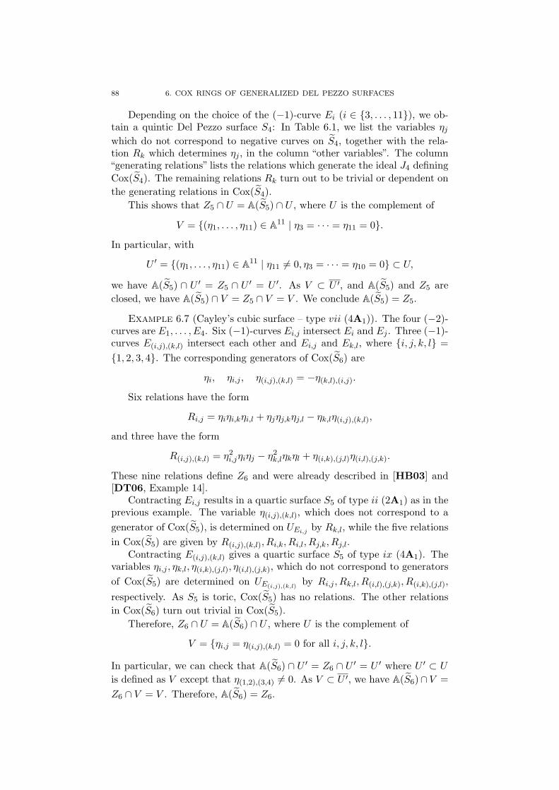
88 6. COX RINGS OF GENERALIZED DEL PEZZO SURFACES
Depending on the choice of the (−1)-curve Ei (i ∈ {3, . . . , 11}), we ob-tain a quintic Del Pezzo surface S4: In Table 6.1, we list the variables ηj
which do not correspond to negative curves on S4, together with the rela-tion Rk which determines ηj , in the column “other variables”. The column“generating relations” lists the relations which generate the ideal J4 definingCox(S4). The remaining relations Rk turn out to be trivial or dependent onthe generating relations in Cox(S4).
This shows that Z5 ∩ U = A(S5) ∩ U , where U is the complement of
V = {(η1, . . . , η11) ∈ A11 | η3 = · · · = η11 = 0}.
In particular, with
U ′ = {(η1, . . . , η11) ∈ A11 | η11 6= 0, η3 = · · · = η10 = 0} ⊂ U,
we have A(S5) ∩ U ′ = Z5 ∩ U ′ = U ′. As V ⊂ U ′, and A(S5) and Z5 areclosed, we have A(S5) ∩ V = Z5 ∩ V = V . We conclude A(S5) = Z5.
Example 6.7 (Cayley’s cubic surface – type vii (4A1)). The four (−2)-curves are E1, . . . , E4. Six (−1)-curves Ei,j intersect Ei and Ej . Three (−1)-curves E(i,j),(k,l) intersect each other and Ei,j and Ek,l, where {i, j, k, l} ={1, 2, 3, 4}. The corresponding generators of Cox(S6) are
ηi, ηi,j , η(i,j),(k,l) = −η(k,l),(i,j).
Six relations have the form
Ri,j = ηiηi,kηi,l + ηjηj,kηj,l − ηk,lη(i,j),(k,l),
and three have the form
R(i,j),(k,l) = η2i,jηiηj − η2
k,lηkηl + η(i,k),(j,l)η(i,l),(j,k).
These nine relations define Z6 and were already described in [HB03] and[DT06, Example 14].
Contracting Ei,j results in a quartic surface S5 of type ii (2A1) as in theprevious example. The variable η(i,j),(k,l), which does not correspond to agenerator of Cox(S5), is determined on UEi,j by Rk,l, while the five relationsin Cox(S5) are given by R(i,j),(k,l), Ri,k, Ri,l, Rj,k, Rj,l.
Contracting E(i,j),(k,l) gives a quartic surface S5 of type ix (4A1). Thevariables ηi,j , ηk,l, η(i,k),(j,l), η(i,l),(j,k), which do not correspond to generatorsof Cox(S5) are determined on UE(i,j),(k,l)
by Ri,j , Rk,l, R(i,l),(j,k), R(i,k),(j,l),respectively. As S5 is toric, Cox(S5) has no relations. The other relationsin Cox(S6) turn out trivial in Cox(S5).
Therefore, Z6 ∩ U = A(S6) ∩ U , where U is the complement of
V = {ηi,j = η(i,j),(k,l) = 0 for all i, j, k, l}.
In particular, we can check that A(S6) ∩ U ′ = Z6 ∩ U ′ = U ′ where U ′ ⊂ U
is defined as V except that η(1,2),(3,4) 6= 0. As V ⊂ U ′, we have A(S6)∩ V =Z6 ∩ V = V . Therefore, A(S6) = Z6.

6.4. DEGREE 4 89
Remark 6.8. In addition to the relations in Jr that we identify in thefirst step of the process (corresponding to the relations in Jr−1 on the onehand, and determining the “other variables” on the other hand), we mightneed further relations in Jr in order to describe A(Sr) on the complementof⋃
(−1)-curves E UE .For example, this happens for the quartic type viii (A3), as we will see
in the following section.
6.4. Degree 4
type singularities lines extra gen. gen. relations0 − 16 − 16 20i A1 12 − 13 10ii 2A1 9 − 11 5iii 2A1 8 − 10 2iv A2 8 − 10 2v 3A1 6 − 9 1vi A2 + A1 6 − 9 1vii A3 5 1 9 1viii A3 4 4 11 5ix 4A1 4 − 8 −x A2 + 2A1 4 − 8 −xi A3 + A1 3 2 9 1xii A4 3 2 9 1xiii D4 2 3 9 1xiv A3 + 2A1 2 1 8 −xv D5 1 3 9 1
Table 6.2. Del Pezzo surfaces of degree 4
Complete results for generalized Del Pezzo surfaces whose degree is atleast 5 can be found in Chapter 5. For smooth Del Pezzo surfaces, see[BP04] and Chapter 3.
In degree 4, Section 5.5 lists all relevant information in the case of DelPezzo surfaces whose universal torsor is an open subset of affine space or ofan affine hypersurface, or equivalently, whose Cox ring has 8 or 9 generators.This includes exactly 10 of the 15 different types. We will describe generatorsand relations for the remaining five types here. We give similar informationas in Chapter 5, using mostly the same notation and conventions.
For S5 of types i to iv, we can check that Cox(S5) is generated by sectionscorresponding to negative curves. Their extended Dynkin diagrams can befound in [CT88, Proposition 6.1].
Type i (A1).• The extended Dynkin diagram consists of one (−2)-curve E0 and
twelve (−1)-curves Ei, Ei,1, Ei,2 for i ∈ {1, . . . , 4}: Ei intersects E0,Ei,1, Ei,2, while Ei,k intersects Ei and Ej,l for j ∈ {1, . . . , 4} \ {i}and l 6= k.

90 6. COX RINGS OF GENERALIZED DEL PEZZO SURFACES
• A basis of Pic(S) is given by E0, . . . , E4, E1,1, with
E2,1 = (0, 1,−1, 0, 0, 1), E3,1 = (0, 1, 0,−1, 0, 1), E4,1 = (0, 1, 0, 0,−1, 1),
E1,2 = (1,−1, 1, 1, 1,−1), E2,2 = (1, 0, 0, 1, 1,−1), E3,2 = (1, 0, 1, 0, 1,−1),
E4,2 = (1, 0, 1, 1, 0,−1),
and −KeS5= (2, 1, 1, 1, 1, 0).
• For i 6= j ∈ {1, . . . , 4}, there is one relation between
η0ηiηj , ηk,1ηl,2, ηl,1ηk,2,
where {i, j, k, l} = {1, . . . , 4}. For i ∈ {1, 2}, there are two relationsbetween
η1η1,i, η2η2,i, η3η3,i, η4η4,i.
This gives 10 relations in total.• 23 monomial sections of −KeS are: η2
0η1η2η3η4, six section of theform ηi,1ηj,1ηk,2ηl,2, twelve section of the form η0ηiηjηi,1ηj,2, foursection of the form η0η
2i ηi,1ηi,2
Type ii (2A1 with 9 lines).
• See Example 6.6.
Type iii (2A1 with 8 lines).
• Its equation is:
x0x1 − x22 = x0x2 + x1x2 + x3x4 = 0
• Singularities: (0 : 0 : 0 : 1 : 0) giving E1, and (0 : 0 : 0 : 0 : 1) givingE2; Lines: E3 = {x0 = x2 = x3 = 0}, E4 = {x0 − x1 = x0 + x2 =x4 = 0}, E5 = {x0−x1 = x0−x2 = x4 = 0}, E6 = {x1 = x2 = x4 =0}, E7 = {x1 = x2 = x3 = 0}, E8 = {x0 − x1 = x0 + x2 = x3 = 0},E9 = {x0 − x1 = x0 − x2 = x3 = 0}, E10 = {x0 = x2 = x4 = 0}.
• A basis of Pic(S) is given by E1, . . . , E6, with
E7 = (−1, 1,−1, 1, 1, 0), E8 = (−1, 1,−1, 1, 0, 1),
E9 = (−1, 1,−1, 0, 1, 1), E10 = (−1, 1,−2, 1, 1, 1),
and −KeS5= (−1, 3,−2, 2, 2, 2).
• Dynkin diagram:
GFED@ABCE1
BBBB
BBBB
1111
1111
1111
111
++++
++++
++++
++++
++++
+++
E3 E10GFED@ABCE2
E7 E6
{{{{{{{{{
E8 E5
����������������
E9 E4
�����������������������

6.4. DEGREE 4 91
• The anticanonical map φ is given by
(φ∗(xi)) = (η(1,1,2,0,0,0)η210, η
(1,1,0,0,0,2)η27, η
(1,1,1,0,0,1)η7η10,
η(2,0,1,0,0,0)η7η8η9, η(0,2,0,1,1,1)η10),
and furthermore, φ∗(x0 − x1) = η(1,1,0,1,1,0)η8η9, φ∗(x0 − x2) =η(1,1,1,1,0,0)η9η10, φ∗(x0 + x2) = η(1,1,1,0,1,0)η8η10, φ∗(x1 + x2) =η(1,1,0,0,1,1)η7η8, φ∗(x2− x1) = η(1,1,0,1,0,1)η7η9, φ∗(x0 + x1 + 2x2) =η(1,1,0,0,2,0)η2
8, φ∗(x0 + x1 − 2x2) = η(1,1,0,2,0,0)η2
9.• Let Z5 be the affine variety defined by
R1 = η3η10 + η6η7 − η5η8
R2 = η3η10 − η6η7 − η4η9
Contracting any line results in a quintic Del Pezzo surface of typei (A1). We see easily that A(S5) = Z5 not only when restricted tothe complement of V = {η3 = · · · = η10 = 0}, but also on V .
Type iv (A2).• Its equation is:
x1x2 − x3x4 = x0(x1 + x2 + x3 + x4)− x3x4 = 0
• Singularities: (1 : 0 : 0 : 0 : 1) giving E1, E2; Lines: E3 = {x0 =x1 = x3 = 0}, E4 = {x0 = x2 = x4 = 0}, E5 = {X = x2 = x3 = 0},E6 = {X = x1 = x4 = 0}, E7 = {X = x2 = x4 = 0}, E8 = {X =x1 = x3 = 0}, E9 = {x0 = x1 = x4 = 0}, E10 = {x0 = x2 = x3 =0}, where X := x1 + x2 + x3 + x4.
• A basis of Pic(S) is E1, . . . , E6, with E7 = (0, 1, 0,−1, 1, 1), E8 =(0, 1,−1, 0, 1, 1), E9 = (1, 2,−1,−1, 2, 1), E10 = (1, 2,−1,−1, 1, 2),and −KeS5
= (2, 4,−1,−1, 3, 3).• Dynkin diagram:
E7 E4
1111
1111
1111
1111
E10 E5
BBBB
BBBB
GFED@ABCE1
||||||||
BBBB
BBBB
GFED@ABCE2
E8 E3
E9 E6
||||||||
• The anticanonical map φ is given by
(φ∗(xi)) = (η(0,0,1,1,0,0)η9η10, η(1,1,0,1,0,1)η7η9, η
(1,1,1,0,1,0)η8η10,
η(1,1,1,0,0,1)η8η9, η(1,1,0,1,1,0)η7η10),
and φ∗(x1 + x3) = η(1,2,0,0,1,2)η9, φ∗(x1 + x4) = η(2,1,0,1,0,0)η27η8,
φ∗(x2+x3) = η(2,1,1,0,0,0)η7η28, φ
∗(x2+x4) = η(1,2,0,0,2,1)η10, φ∗(x1+x2 + x3 + x4) = η(2,2,0,0,1,1)η7η8.
• Contracting one of E5, E6, E7, E8, we get a quintic surface of typei (A1). For one of E3, E4, E9, E10, we obtain a quintic surface oftype iii (A2).

92 6. COX RINGS OF GENERALIZED DEL PEZZO SURFACES
• Let Z5 be the affine variety defined by
R1 = η6η9 + η5η10 − η1η7η8,
R2 = η4η7 + η3η8 − η2η5η6.
On the complement U of V = {η3 = · · · = η10 = 0}, we haveA(S5) = Z5. For U ′ = {η3 6= 0, η4 = · · · = η10 = 0} ⊂ U , we haveA(S5) ∩ U ′ = Z5 ∩ U ′ = U ′. Therefore, A(S5) ∩ V = V , whichcoincides with Z5 ∩ V , and we obtain A(S5) = Z5.
Type viii (A3).
• When we contract any of the four (−1)-curves S5, we obtain theminimal desingularization S4 of a quintic Del Pezzo surface S4 oftype iii (A2), where Cox(S4) has two extra generators α1, α2. Intotal, we obtain four extra generators of Cox(S5).
• Its equation is:
x0x1 − x22 = (x0 + x1 + x3)x3 − x2x4 = 0
• Singularities: (0 : 0 : 0 : 0 : 1) giving E1, E2, E3; Lines: E4 = {x0 =x2 = x3 = 0}, E5 = {x1 = x2 = x3 = 0}, E6 = {x0 = x2 =x1 + x3 = 0}, E7 = {x1 = x2 = x0 + x3 = 0}
• A basis of Pic(S) is E1, . . . , E6, with E7 = (−1, 0, 1,−1, 1, 1), and−KeS5
= (1, 2, 3, 0, 2, 2).• Dynkin diagram:
E4
AAAA
AAAA
UUUUUUUUUUUUUUUUUUUUUUUU A1
PPPPPPPPPPPPPPPP
UUUUUUUUUUUUUUUUUUUUUUUU A2 E6
BBBB
BBBB
GFED@ABCE1
||||||||
UUUUUUUUUUUUUUUUUUUUUUUU E7
~~~~~~~~
iiiiiiiiiiiiiiiiiiiiiiiiA4
nnnnnnnnnnnnnnnn
iiiiiiiiiiiiiiiiiiiiiiiiA3 E5
GFED@ABCE3
GFED@ABCE2
iiiiiiiiiiiiiiiiiiiiiiii
• The anticanonical map φ is given by
(φ∗(xi)) = (η(1,2,3,0,2,2), η(3,2,1,2,0,0)η27, η
(2,2,2,1,1,1)η7, η(1,1,1,0,1,0)η7α1, α1α4),
and furthermore, φ∗(x1 + x3) = η(1,1,1,0,0,1)η7α2, φ∗(x0 + x3) =η(1,1,1,1,1,0)α3, φ∗(x0+x1+x3) = η(1,1,1,1,0,1)α4, φ∗(x2+x4) = α2α3.
• Relations: Let V5 ⊂ A11 be the affine variety defined by the fiverelations
R1 = η21η2η
24η7 + η5α1 − η6α2,
R2 = η2η23η
25η6 + η7α2 − η4α4,
R3 = η2η23η5η
26 + η7α1 − η4α3,
R4 = η21η2η4η
27 + η5α3 − η6α4,
R5 = η21η
22η
23η4η5η6η7 + α1α4 − α2α3.
Note that R1, . . . , R4 correspond to the relation in Cox(S4) whencontracting E4, . . . , E7, respectively. Therefore, Cox(S5) is given by
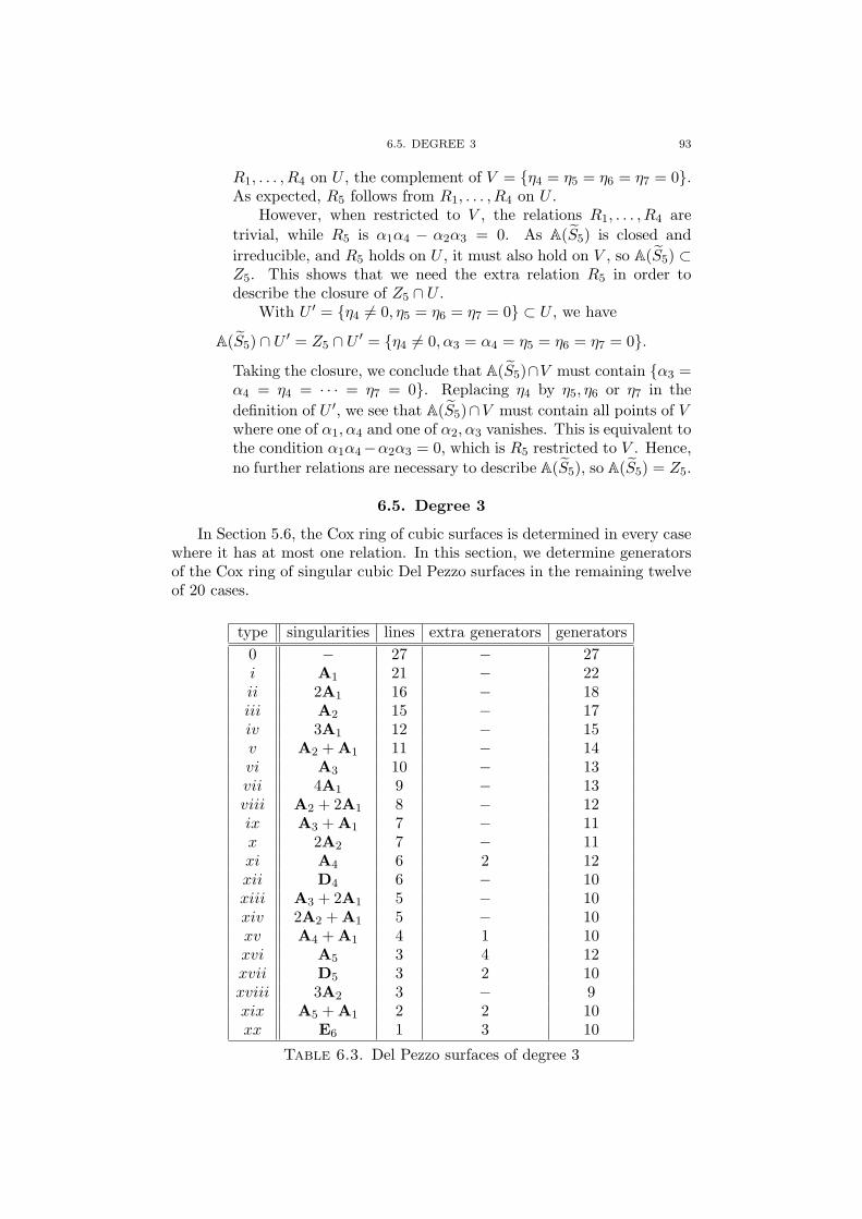
6.5. DEGREE 3 93
R1, . . . , R4 on U , the complement of V = {η4 = η5 = η6 = η7 = 0}.As expected, R5 follows from R1, . . . , R4 on U .
However, when restricted to V , the relations R1, . . . , R4 aretrivial, while R5 is α1α4 − α2α3 = 0. As A(S5) is closed andirreducible, and R5 holds on U , it must also hold on V , so A(S5) ⊂Z5. This shows that we need the extra relation R5 in order todescribe the closure of Z5 ∩ U .
With U ′ = {η4 6= 0, η5 = η6 = η7 = 0} ⊂ U , we have
A(S5) ∩ U ′ = Z5 ∩ U ′ = {η4 6= 0, α3 = α4 = η5 = η6 = η7 = 0}.
Taking the closure, we conclude that A(S5)∩V must contain {α3 =α4 = η4 = · · · = η7 = 0}. Replacing η4 by η5, η6 or η7 in thedefinition of U ′, we see that A(S5)∩V must contain all points of Vwhere one of α1, α4 and one of α2, α3 vanishes. This is equivalent tothe condition α1α4−α2α3 = 0, which is R5 restricted to V . Hence,no further relations are necessary to describe A(S5), so A(S5) = Z5.
6.5. Degree 3
In Section 5.6, the Cox ring of cubic surfaces is determined in every casewhere it has at most one relation. In this section, we determine generatorsof the Cox ring of singular cubic Del Pezzo surfaces in the remaining twelveof 20 cases.
type singularities lines extra generators generators0 − 27 − 27i A1 21 − 22ii 2A1 16 − 18iii A2 15 − 17iv 3A1 12 − 15v A2 + A1 11 − 14vi A3 10 − 13vii 4A1 9 − 13viii A2 + 2A1 8 − 12ix A3 + A1 7 − 11x 2A2 7 − 11xi A4 6 2 12xii D4 6 − 10xiii A3 + 2A1 5 − 10xiv 2A2 + A1 5 − 10xv A4 + A1 4 1 10xvi A5 3 4 12xvii D5 3 2 10xviii 3A2 3 − 9xix A5 + A1 2 2 10xx E6 1 3 10
Table 6.3. Del Pezzo surfaces of degree 3
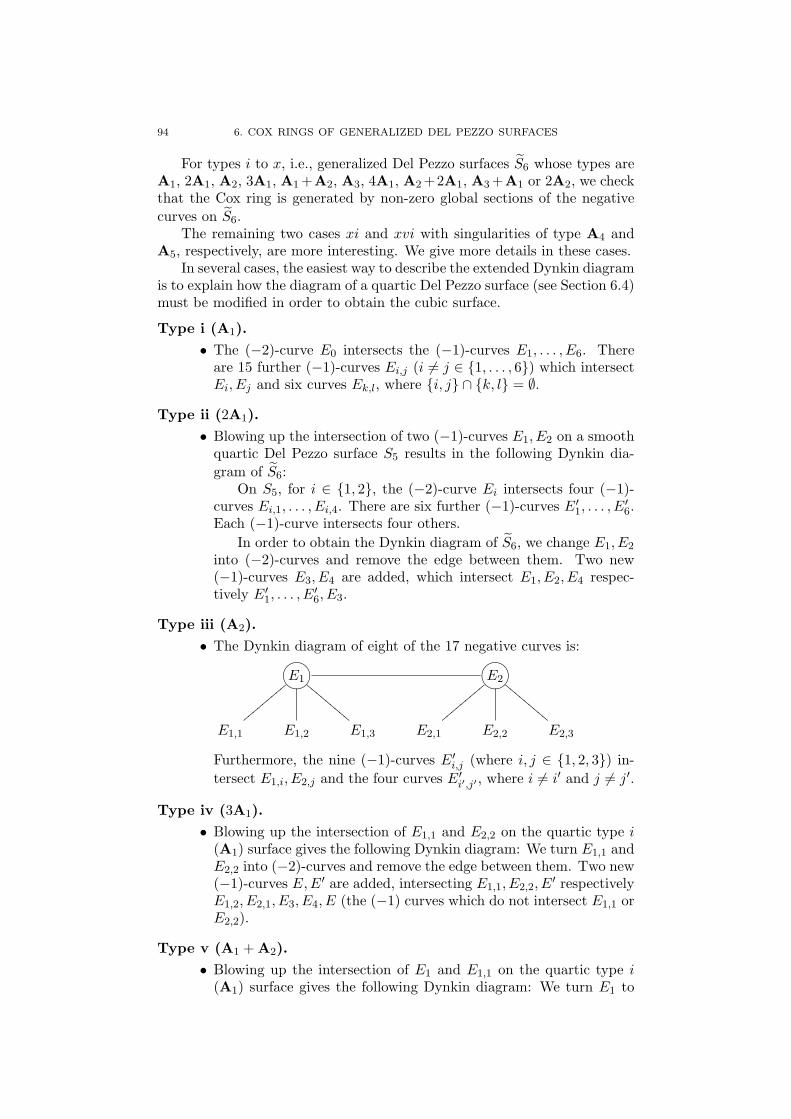
94 6. COX RINGS OF GENERALIZED DEL PEZZO SURFACES
For types i to x, i.e., generalized Del Pezzo surfaces S6 whose types areA1, 2A1, A2, 3A1, A1 +A2, A3, 4A1, A2 +2A1, A3 +A1 or 2A2, we checkthat the Cox ring is generated by non-zero global sections of the negativecurves on S6.
The remaining two cases xi and xvi with singularities of type A4 andA5, respectively, are more interesting. We give more details in these cases.
In several cases, the easiest way to describe the extended Dynkin diagramis to explain how the diagram of a quartic Del Pezzo surface (see Section 6.4)must be modified in order to obtain the cubic surface.
Type i (A1).• The (−2)-curve E0 intersects the (−1)-curves E1, . . . , E6. There
are 15 further (−1)-curves Ei,j (i 6= j ∈ {1, . . . , 6}) which intersectEi, Ej and six curves Ek,l, where {i, j} ∩ {k, l} = ∅.
Type ii (2A1).• Blowing up the intersection of two (−1)-curves E1, E2 on a smooth
quartic Del Pezzo surface S5 results in the following Dynkin dia-gram of S6:
On S5, for i ∈ {1, 2}, the (−2)-curve Ei intersects four (−1)-curves Ei,1, . . . , Ei,4. There are six further (−1)-curves E′
1, . . . , E′6.
Each (−1)-curve intersects four others.In order to obtain the Dynkin diagram of S6, we change E1, E2
into (−2)-curves and remove the edge between them. Two new(−1)-curves E3, E4 are added, which intersect E1, E2, E4 respec-tively E′
1, . . . , E′6, E3.
Type iii (A2).• The Dynkin diagram of eight of the 17 negative curves is:
GFED@ABCE1
zzzz
zzzz
z
DDDD
DDDD
DGFED@ABCE2
zzzz
zzzz
z
DDDD
DDDD
D
E1,1 E1,2 E1,3 E2,1 E2,2 E2,3
Furthermore, the nine (−1)-curves E′i,j (where i, j ∈ {1, 2, 3}) in-
tersect E1,i, E2,j and the four curves E′i′,j′ , where i 6= i′ and j 6= j′.
Type iv (3A1).• Blowing up the intersection of E1,1 and E2,2 on the quartic type i
(A1) surface gives the following Dynkin diagram: We turn E1,1 andE2,2 into (−2)-curves and remove the edge between them. Two new(−1)-curves E,E′ are added, intersecting E1,1, E2,2, E
′ respectivelyE1,2, E2,1, E3, E4, E (the (−1) curves which do not intersect E1,1 orE2,2).
Type v (A1 + A2).• Blowing up the intersection of E1 and E1,1 on the quartic type i
(A1) surface gives the following Dynkin diagram: We turn E1 to

6.5. DEGREE 3 95
E1,1 into (−2)-curves and remove the edge between them. A new(−1)-curve E intersects E1 and E1,1.
Type vi (A3).
• The extended Dynkin diagram is the following modification of thediagram of quartic type ii (2A1 with 9 lines), corresponding tothe blow-up of a point on E3: The (−1)-curve E3 is changed to a(−2)-curve. Two new (−1)-curves E and E′ are added, where Eintersects E3, E
′, and E′ intersects E8, E9, E10, E11, E.
Type vii (4A1).
• See Example 6.7.
Type viii (A2 + 2A1).
• Dynkin diagram:
GFED@ABCE2
QQQQQQQQQQQQQQQQ GFED@ABCE1
BBBB
BBBB
E7
||||||||
1111
1111
1111
111 E9
mmmmmmmmmmmmmmmmmE5 E12 E8
E10 E6
GFED@ABCE4 E11GFED@ABCE3
Type ix (A3 + A1).
• Dynkin diagram:
GFED@ABCE4 E8
@@@@
@@@@
@
E9 E6
0000
0000
0000
0000
GFED@ABCE1
E5
����������������
AAAA
AAAA
E10 E7GFED@ABCE2
E11GFED@ABCE3
Type x (2A2).
• See Section 6.6.
Type xi (A4).

96 6. COX RINGS OF GENERALIZED DEL PEZZO SURFACES
• Dynkin diagram:
E5GFED@ABCE2
GFED@ABCE3GFED@ABCE4
GFED@ABCE1
|||||||||E9 E7
|||||||||E8
E6
{{{{{{{{E10
{{{{{{{{
• We claim that Cox(S6) is generated by η1, . . . , η10 and α1, α2, whereA1 := deg(α1) intersects E5, E7, E9, A2 and twice E10, while A2 :=deg(α2) intersects E5, E8, E10, A1 and twice E9. This is checked byconsidering the Cox(S5) for the various quartic contractions S5 ofthe (−1)-curves on S6:
(−1)-curve type of S5 extra curves on S5 corresp. curves on S6
E5 vi : A2 + A1 − −E6 viii : A3 A1, A2, A3, A4 A1, E10, A2, E9
E7 vii : A3 A A2
E8 vii : A3 A A1
E9 xii : A4 A1, A2 A2, E6
E10 xii : A4 A1, A2 A1, E6
Type xvi (A5).• Dynkin diagram:
GFED@ABCE1GFED@ABCE2
GFED@ABCE3GFED@ABCE4
GFED@ABCE5 E6
E7 E8
• Contracting E6 gives a quartic surface S5 with a singularity of typeA4. We have two extra generators α1, α2 of degree A1, A2 whichintersect E7 and twice E8 respectively E1 and E8. Contracting E8
gives the same type of quartic surface. Here, the extra generatorsintersect E7 and twice E6 respectively E1 and E6. This shows thatwe need four extra generators α1, . . . , α4 such that the correspond-ing divisors A1, . . . , A4 intersect one of E1, E7 and one of E6, E8.
Contracting E7 gives a quartic surface with singularities A3 +A1. Its Cox ring also has two extra generators, but the inducedsections of S6 are two of α1, . . . , α4 as above.
• Therefore, Cox(S6) is generated by these 12 elements. By consider-ing the sections in degrees Ai, we see that it is a minimal generatingset (cf. Lemma 2.5).
6.6. Families of Del Pezzo surfaces
In this section we compute the Cox ring of a family of Del Pezzo sur-faces. By Example 1.36, there is a one-parameter family of singular Del

6.6. FAMILIES OF DEL PEZZO SURFACES 97
Pezzo surfaces S of type 2A2. Its extended Dynkin diagram is given inExample 1.32.
We have dim(H0(l0 − l5)) = 2, but
l0 − l5 = E4 + E6 + 2E7 = E1 + E11 = E2 + E8 = E3 + E9.
Hence, there are two relations between
η4η6η27, η1η11, η2η8, η3η9,
where ηi is a non-zero element of H0(Ei). To determine the relation betweenthese sections, note that
η4η5η6η27, η1η5η11, η2η5η8, η3η5η9 ∈ H0(S6, l0)
are π∗(s7), . . . , π∗(s10) under the map π : S6 → P2, with si ∈ H0(P2,OP2(1))is a section vanishing in Ei for i ∈ {7, . . . , 10}. By our choice of E7, . . . , E10
in P2 as in (1.1), depending on the parameter α, two relations betweens7, . . . , s10 are
s9 + s8 − s7 = 0 and s10 + αs8 − s7 = 0.
This gives rise to two relations in H0(S6, l0), which results in relations inH0(S6, l0 − l5) after dividing by η5:
R1(ηi) := η2η8 +η1η11−η4η6η27 = 0, R2(ηi) := η3η9 +αη1η11−η4η6η
27 = 0.
Note that the contraction of the (−1)-curve E7 on S6 results in a gen-eralized quartic Del Pezzo surface S5 of type 2A1 (with 8 lines), while thecontraction of any other (−1)-curve gives S5 of type A2 + A1. As before,we can check by comparing the generators η1, . . . , η11 and the relations R1,R2 with the results in these two quartic types that we have
Cox(S6) = K[η1, . . . , η11]/(R1(ηi), R2(ηi)).
Our method of determining the Cox ring shows that the following prop-erties are invariant in families of isomorphy classes S of the same type:
• By definition, the extended Dynkin diagram and the Picard group.• The numbers and degrees of the generators of Cox(S) in Pic(S)
(see Lemma 2.5).• The numbers and degrees of the relations in Pic(S).
However, the exact form of the relations depends on the choice of isomorphyclass in the family. As the monomials occurring in a relation are determinedby the degrees of the relation and the generators, only the coefficients vary.
See also Section 5.6 for the two isomorphy classes of type D4 in degree 3.

Part 2
Rational points on Del Pezzosurfaces


CHAPTER 7
Manin’s conjecture
7.1. Introduction
Let f ∈ Z[x0, . . . , xn] be a non-singular form of degree d. By the circlemethod,
N(f,B) := #{x ∈ Zn+1/± | maxj
(|xj |) ≤ B} ∼ c ·Bn+1−d
(where x ∈ Zn+1/± means that we identify x with −x = (−x0, . . . ,−xn))with c ∈ R>0, provided that n > 2d · (d − 1), and f(x) = 0 has solutionsover all completions of Q (see [Bir62]). Let X = Xf ⊂ Pn be the smoothhypersurface over Q, given by f(x) = 0. It follows that
(7.1) NX,H−KX(B) := #{x ∈ X(Q) | H−KX
(x) ≤ B} ∼ C ·B,
as B → ∞. Here X(Q) is the set of rational points on X, represented byprimitive vectors x ∈ (Zn+1
prim \ 0)/± (i.e., x = (x0, . . . , xn) is identified with−x, and there is no prime dividing all coordinates x0, . . . , xn), and
(7.2) H−KX(x) := max
j(|xj |)n+1−d, for x = (x0, . . . , xn) ∈ (Zn+1
prim \ 0)/±
is the anticanonical height of a primitive representative.The main goal of Manin’s program on the distribution of rational points
of bounded height (see [FMT89] and [BM90]) is an extension of the asymp-totic formula (7.1) to Fano varieties which are not necessarily isomorphic tohypersurfaces in projective space. A Fano variety is a projective varietywhose anticanonical class is ample.
It became apparent that, in general, to obtain a geometric interpreta-tion of asymptotic results, it may be necessary to restrict to appropriateZariski open subsets U of X. Otherwise, the number of rational points ona Zariski closed subset of lower dimension may dominate the total numberof rational points; e.g., this phenomenon occurs for smooth and for singularcubic surfaces where the number of rational points on rational lines on sucha surface dominates the total number of rational points. Hence, we countrational points on the complement of these lines. It is often necessary toconsider rational points in finite extensions of the rationals: while X(Q)might be empty, X(k) could still contain infinitely many points for somenumber field k.
We are concerned with Del Pezzo surfaces, cf. Chapter 1 for their basicproperties. Smooth Del Pezzo surfaces are birational to P2, provided theground field is algebraically closed. Besides P1 × P1, they are blow-ups ofP2 in at most eight points in general position.
101
102 7. MANIN’S CONJECTURE
Of special interest are irreducible curves for which the self intersectionnumber is negative, which are called negative curves (Definition 1.20). Arith-metically, rational points tend to accumulate on negative curves where theyare easy to count. Our main focus is to count rational points on the com-plement of the negative curves.
For smooth Del Pezzo surfaces of degree ≥ 3, the negative curves areexactly the lines (in the anticanonical embedding, see Remark 1.13), havingself intersection number −1.
Singular Del Pezzo surfaces are obtained as described in Section 1.5. Weblow up P2 in points in almost general position (see Definition 1.20; e.g.,three points on a line). This results in a generalized Del Pezzo surface, i.e.,a smooth surface S containing negative curves with self intersection number−2 (called (−2)-curves). Contracting the (−2)-curves gives a singular DelPezzo surface S whose singularities are rational double points and whoseminimal desingularization is S.
For number fields, we say that a Del Pezzo surface is split if all of thenegative curves are defined over that ground field, in which case the surfaceis birational to P2. There do exist non-split Del Pezzo surfaces which are bi-rational to P2 over that ground field; however, the generic Del Pezzo surfaceis non-split and is not birational to P2 over the ground field.
From here, we work over Q. Manin’s conjecture in the special case ofsmooth or singular Del Pezzo surfaces Srof degree 9−r ≥ 3 can be formulatedas follows. Consider Sr as a subvariety of P9−r using the anticanonicalembedding (Remark 1.13 and Remark 1.26). For the height function onP9−r(Q), we always use
H(x) := max(|x0|, . . . , |x9−r|),with x ∈ P9−r(Q) represented by integral coprime coordinates x0, . . . , x9−r.For an open subset U of S, let
NU,H(B) := #{x ∈ S(Q) | H(x) ≤ B}.Conjecture 7.1. Let S be a smooth or singular Del Pezzo surface over
Q. Then there exists a subset U ⊂ S which is dense and open in the Zariskitopology such that
(7.3) NU,H(B) ∼ cS,H ·B(logB)t−1,
as B → ∞, where t is the rank of the Picard group over Q of the minimaldesingularization S of S.
The constant cS,H has been defined by Peyre [Pey95]; see Section 7.2for more details. It should be non-zero if S(Q) 6= ∅. It is analogous to thesingular series and the singular integral that you meet in the classical circlemethod. Note that a line defined over Q on a Del Pezzo surface of degree≥ 3 contributes ∼ c · B2 rational points to the counting function (for somepositive constant c). Thus it is expected that U is the complement to alllines defined over Q (i.e., the negative curves).
Table 7.1 gives an overview of current results towards Conjecture 7.1for Del Pezzo surfaces. In Column 4 (“type of result”), “asymptotic” meansthat the analog of (7.3) is established, including the predicted value of theconstant; “bounds”means that only upper and lower bounds of the expected

7.1. INTRODUCTION 103
order of magnitude B(logB)t are known. As explained in Definition 1.28,the type of a surface is usually denoted by the Dynkin diagram associatedto its singularities.
degree singularities (non-)split type of result reference≥ 6 – split asymptotic [BT98]5 – split asymptotic [Bre02]5 – non-split asymptotic [BF04]4 D5 split asymptotic [CLT02], [BB04]4 D4 non-split asymptotic [BB05]4 D4 split asymptotic Chapter 104 3A1 split bounds [Bro05]4 2A1 non-split asymptotic de la Breteche,
Browning, Peyre3 3A2 split asymptotic [BT98], [Bre98], . . .3 4A1 split bounds [HB03]3 D4 split bounds [Bro04]3 E6 split asymptotic Chapter 9, [BBD05]
Table 7.1. Results for Del Pezzo surfaces
The paper [BT98] contains a proof of Manin’s conjecture for toric Fanovarieties. This includes all smooth Del Pezzo surfaces of degree ≥ 6 andthe 3A2 cubic surface. A list of all types of toric Del Pezzo surfaces can befound in Table 1.4.
Figure 7.1 shows all points of height ≤ 50 on the Cayley cubic surface(Example 6.7), which has four singularities of type A1 and was consideredin [HB03].
The proofs of Manin’s conjecture proceed either via the height zeta func-tion
ZU,H(s) :=∑
x∈U(Q)
H−KX(x)−s,
whose analytic properties are related to the asymptotic (7.3) by Tauberiantheorems (see Section 7.3), or via the lifting of the counting problem tothe universal torsor – an auxiliary variety parameterizing rational points.Experience shows that counting points on the universal torsor is often eas-ier. The torsor approach was developed by Colliot-Thelene and Sansuc inthe context of the Brauer-Manin obstruction [CTS87] and was applied toManin’s conjecture by Peyre [Pey98] and Salberger [Sal98].
In the simplest case of hypersurfaces X = Xf ⊂ Pn over Q, with n ≥ 4,this is exactly the passage from rational vectors x = (x0, . . . , xn), modulothe diagonal action of Q∗, to primitive lattice points (Zn+1
prim \0)/±. Geomet-rically, we have
An+1 \ {0} Gm−−−−→ Pn and TXGm−−−−→ X.
Here, TX is the hypersurface in An+1 \ {0} defined by the form f . The 1-dimensional torus Gm is interpreted as the Neron-Severi torus TNS(X) (seeSection 2) since Pic(X) has rank 1. Rational points on the base surface Xare lifted to integral points on the torsor, modulo the action of the group
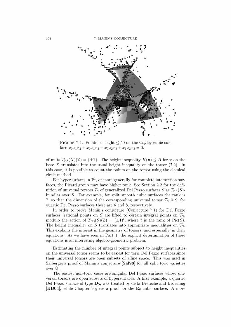
104 7. MANIN’S CONJECTURE
Figure 7.1. Points of height ≤ 50 on the Cayley cubic sur-face x0x1x2 + x0x1x3 + x0x2x3 + x1x2x3 = 0.
of units TNS(X)(Z) = {±1}. The height inequality H(x) ≤ B for x on thebase X translates into the usual height inequality on the torsor (7.2). Inthis case, it is possible to count the points on the torsor using the classicalcircle method.
For hypersurfaces in P3, or more generally for complete intersection sur-faces, the Picard group may have higher rank. See Section 2.2 for the defi-nition of universal torsors TS of generalized Del Pezzo surfaces S as TNS(S)-bundles over S. For example, for split smooth cubic surfaces the rank is7, so that the dimension of the corresponding universal torsor TS is 9; forquartic Del Pezzo surfaces these are 6 and 8, respectively.
In order to prove Manin’s conjecture (Conjecture 7.1) for Del Pezzosurfaces, rational points on S are lifted to certain integral points on TS ,modulo the action of TNS(S)(Z) = (±1)t, where t is the rank of Pic(S).The height inequality on S translates into appropriate inequalities on TS .This explains the interest in the geometry of torsors, and especially, in theirequations. As we have seen in Part 1, the explicit determination of theseequations is an interesting algebro-geometric problem.
Estimating the number of integral points subject to height inequalitieson the universal torsor seems to be easiest for toric Del Pezzo surfaces sincetheir universal torsors are open subsets of affine space. This was used inSalberger’s proof of Manin’s conjecture [Sal98] for all split toric varietiesover Q.
The easiest non-toric cases are singular Del Pezzo surfaces whose uni-versal torsors are open subsets of hypersurfaces. A first example, a quarticDel Pezzo surface of type D5, was treated by de la Breteche and Browning[BB04], while Chapter 9 gives a proof for the E6 cubic surface. A more

7.2. PEYRE’S CONSTANT 105
detailed analysis of this surface, which gives a much improved error termin the asymptotic, can be found in a separate paper (joint with R. de laBreteche and T. D. Browning [BBD05], see also Section 7.3).
While in principle, a similar approach seems possible for the other sur-faces whose universal torsors are hypersurfaces, it does not seem to be easyto count the points on the universal torsor using methods of analytic numbertheory. The first step of passing to the universal torsor can be done usingthe detailed information on the Cox ring given in Chapter 5 for all singularDel Pezzo surfaces of degree ≥ 3 which have such a universal torsor. Oneexample which can be treated is a split quartic Del Pezzo surface of typeD4, see Chapter 10.
However, new difficulties seem to arise in the estimation of error termsin many other cases. Apparently, it is easier for Del Pezzo surfaces of higherdegree. In each degree, the easiest cases seem to be the ones with the“worst”singularities, e.g., D5 in degree 4 and E6 in degree 3. Therefore, the nextchallenge would be to prove Manin’s conjecture for a singular Del Pezzosurface of degree 2, or for other singular cubic surfaces.
7.2. Peyre’s constant
In this section, we explain the leading constant cS,H appearing in Con-jecture 7.1 for a smooth Del Pezzo surface S defined over a number field K.It was suggested by Peyre [Pey95], Batyrev and Tschinkel [BT95] and isdefined as the product
cS,H := α(S) · β(S) · ωH(S)
of the following three constants.The first factor α(S) is related to a certain volume in the effective cone
Λeff(S) in the Picard group Pic(S). Note that the ground field is not neces-sarily algebraically closed, so the rank of Pic(S) could be lower than r + 1if S is a Del Pezzo surface of degree 9− r. For its precise definition and itscalculation in the case of split Del Pezzo surfaces, see Chapter 8 below.
The second factor β(S) is defined as the order of the Galois cohomologygroup
H1(K,Pic(S)) := H1(Gal(K/K),Pic(S)K).
It first appeared in [BT95] and [BT98, Section 1]. We have β(S) = 1 forsplit Del Pezzo surfaces.
For singular Del Pezzo surfaces, we must replace α(S) and β(S) by α(S)and β(S) for the minimal desingularization S of S.
Example 7.2. Consider a singular quartic Del Pezzo surface S with twoconjugate singularities which are not joined by a line on S. Such a surface iscalled Iskovskih surface (cf. [CT88, Section 7]). Its type is 2A1 (with eightlines). In yet unpublished work of de la Breteche, Browning, and Peyre,Manin’s conjecture is proved for an Iskovskih surface S with β(S) > 1.
The third factor ωH(S) does not only depend on the surface S, but alsoon the height function H. If the ground field is K = Q, it is defined as the
106 7. MANIN’S CONJECTURE
product
ωH(S) = lims→1
((s− 1)rkPic(S)L(s,Pic(S)))ω∞(S)∏p
ωp(S)Lp(1,Pic(S))
.
Here, ω∞(S) is the “density of points over R” and can be calculated by[Pey95, Section 5.1] as follows using the Leray form if S is a completeintersection: Suppose the anticanonical embedding of S is given by m formsf1, . . . , fm ∈ Z[x0, . . . , xN ] in PN such that the matrix
M(x) :=(∂fi
∂xj(x))
1≤i≤m,N−m+1≤j≤N
is invertible. Then
ω∞(S) =∫|x0|,...,|xN |≤1
M(x)−1dx0 . . .dxN−m.
For each prime p, the constant ωp(S) is the “p-adic density” of pointson S. It can be calculated using the Leray measure [Pey95, Lemma 5.4.6].For complete intersections S in projective space PN , defined by m formsf1, . . . , fm ∈ Z[x0, . . . , xN ], [PT01a, Proposition 3.1] gives the followingpossibility of its explicit calculation:
ωp(S) = limn→∞
#{x ∈ (Z/pnZ)N+1 | (f1(x), . . . , fm(x)) = 0 ∈ (Z/pnZ)m}pn·(dim S+1)
.
By Remark 1.13 and Remark 1.26, this includes the smooth and singularcubic and quartic Del Pezzo surfaces Sr, where m = 1, N = 3 in the cubiccase, and m = 2, N = 4 in the quartic case. See [BB04] for an example ofits calculation.
For the definition of the L-functions occuring in the definition of ωH(S),see [Pey95, Section 2.2]. In the split case, we have
lims→1
((s− 1)rkPic(S)L(s,Pic(S)) = lims→1
((s− 1)r+1ζ(s)r+1) = 1
andLp(1,Pic(S))−1 = (1− 1/p)r+1.
For a singular Del Pezzo surface S with minimal desingularization S, wecalculate ωH(S), where the anticanonical image of S coincides with theanticanonical embedding of S.
7.3. Height zeta functions
Let S be a smooth or singular Del Pezzo surface whose minimal desingu-larization is the generalized Del Pezzo surface S (with S = S in the smoothcase). For simplicity, we assume that S is split over Q, with height functionH : S(Q) → R. Let U be the complement of the lines on S.
Definition 7.3. The height zeta function ZU,H of S is defined for alls ∈ C with real part <e(s) > 1 as
ZU,H(s) :=∑
x∈U(Q)
1H(x)s
.

7.3. HEIGHT ZETA FUNCTIONS 107
Conjecture 7.1 is related to properties of the height zeta function in thefollowing way by Tauberian theorems:
• IfNU,H(B) ∼ cS,H ·B(logB)t−1,
then ZU,H(s) should have a pole of order t at s = 1 with residue(t− 1)! · cS,H .
• If we can prove Conjecture 7.1 with an error term of order B1−δ
for some δ > 0, i.e., if
NU,H(B) = cS,H ·BQ(logB) +O(B1−δ),
where Q is a monic polynomial of degree r−1, then ZU,H(s) shouldhave a meromorphic continuation to the halfplane
{s ∈ C | <e(s) > 1− δ}.Our proofs of Manin’s conjecture for a cubic surface of type E6 in Chap-
ter 9 and a quartic surface of type D4 in Chapter 10 give error terms of orderO(B(logB)2) respectively O(B(logB)3). This does not yield information onthe properties of ZU,H(s) for <e(s) < 1.
However, in joint work with de la Breteche and Browning [BBD05], weprove the following result:
Theorem 7.4. Let S be the cubic surface of type E6 as in (9.1), and letU be the complement of the unique line on S. Then
NU,H(B) = cS,H ·BQ(logB) +Oε(B10/11+ε),
where Q is a monic polynomial of degree 6, and cS,H is the constant predictedby Peyre.
Proof. [BBD05, Theorem 1]. �
In fact, we prove a stronger statement than a meromorphic continuationof ZU,H(s) to <e(s) > 10/11:
Theorem 7.5. For S and U as in Theorem 7.4, (s− 1)7 ·ZU,H(s) has aholomorphic continuation to the halfplane <e(s) > 9/10.
Proof. [BBD05, Theorem 2]. �


CHAPTER 8
On a constant arising in Manin’s conjecture
8.1. Introduction
For 1 ≤ r ≤ 8, let Sr be a smooth Del Pezzo surface of degree 9− r (seeSection 1.3). Suppose that Sr is split over Q.
An important object associated to Sr is the effective cone Λeff(Sr) (seeDefinition 1.8), i.e., the closed convex cone in
Pic(Sr)R := Pic(Sr)⊗Z R
which is generated by the classes of effective divisors. For r ≥ 2, Λeff(Sr) isgenerated by the classes of the (−1)-curves by Lemma 1.15. As always, weidentify Pic(Sr)R and its dual using the intersection form.
This chapter, whose results first appeared in [Der06a], is concerned withthe constant α(Sr) appearing in the leading constant of Manin’s conjecture,cf. Section 7.2. Its definition is due to Peyre [Pey95, Definition 2.4]; see[PT01b, Section 6] for more details.
Definition 8.1. Let Λeff(Sr) be the effective cone, Λ∨eff(Sr) its dual, and−KSr the anticanonical class on Sr. Then we define
α(Sr) := Vol(Pr),
wherePr := {x ∈ Λ∨eff(Sr) | (−KSr , x) = 1},
and the Lebesgue measure on the hyperplane
{x ∈ Pic(Sr)R | (−KSr , x) = 1}is defined by the r-form dx such that dx ∧ dω = dy, where dy is the formcorresponding to the natural Lebesgue measure on Pic(Sr)R and dω is thelinear form defined by −KSr on Pic(Sr)R.
For small r, the calculation of α(Sr) can be carried out directly by hand(see [Bre02, Section 1.3] for the case r = 4). For larger r, especially r = 8,a direct calculation seems to be currently impossible even with the helpof software like Polymake [GJ00]. In this case, the cone Λeff(S8) has 240generators, while Λ∨eff(S8) has 19440 generators. A direct calculation ofα(S8) would require a triangulation of Λ∨eff(S8), which seems to be out ofreach for today’s software and hardware.
Therefore, we need a more detailed knowledge of Λ∨eff(Sr). See Sec-tion 1.4 for details on the action of the Weyl group Wr on Pic(Sr). Ourmain result which will allow us to compute α(Sr) recursively is:
Theorem 8.2. For r ≥ 3, the nef cone Λ∨eff(Sr) has Nr faces, where Nr
is the number of (−1)-curves on Sr. Each face is isomorphic to Λ∨eff(Sr−1).
109
110 8. ON A CONSTANT ARISING IN MANIN’S CONJECTURE
The Weyl group Wr acts transitively on the faces and fixes −KSr in theinterior of Λ∨eff(Sr).
This observation is a crucial step in the proof of the following recursiveformula for α(Sr); see Table 8.1 for the values of α(Sr) and Nr.
Theorem 8.3. Let Sr be a split smooth Del Pezzo surface of degree 9−r.We have α(S2) = 1/24 and
α(Sr) =Nr · α(Sr−1)r · (9− r)
for 3 ≤ r ≤ 8. Furthermore, α(S1) = 1/6, α(P1×P1) = 1/4, and α(P2) = 1.
r 2 3 4 5 6 7 8Nr 3 6 10 16 27 56 240α(Sr) 1/24 1/72 1/144 1/180 1/120 1/30 1
Table 8.1. Smooth Del Pezzo surfaces
Next, we consider split singular Del Pezzo surfaces S′r (see Section 1.5)with minimal desingularizations S′r of degree 9−r. The definition of α(S′r) isalmost the same as for smooth Del Pezzo surfaces: we must consider −KeSr
,
Λeff(S′r) and Λ∨eff(S′r) in Pic(S′r) of rank r+1. We will see in Proposition 8.11that Λeff(S′r) is generated by the negative curves, including (−2)-curves, inthis case.
As explained in Section 1.4, negative curves on S′r are related to the (−1)-curves on a smooth Del Pezzo surface Sr of the same degree and certain rootsystems in Pic(Sr)R.
More precisely, recall that, for r ≥ 2, we can identify Pic(S′r) and Pic(Sr)together with the intersection form and the anticanonical classes −KeS′
rand
−KSr . Then the (−2)-curves of S′r are the simple roots ∆ of a root systemΦ in Pic(Sr)R, and the (−1)-curves of S′r are the (−1)-curves of Sr whichlie in the fundamental chamber C0 of Φ.
The root system Φ is the direct sum of the irreducible root systemsassociated to the singularities of S′r. Let W be the Weyl group associatedto Φ, generated by the reflections sE associated to the (−2)-curves E. Thespace Pic(Sr)R is the union of chambers Cw := w(C0) for all w ∈ W , wherethe intersection of two chambers has lower dimension.
This description of the negative curves on S′r in terms of (−1)-curves onthe smooth Del Pezzo surface Sr of the same degree and the action of theWeyl group W leads us to the following result on the structure of the nefcone Λ∨eff(S′r) of S′r:
Theorem 8.4. For r ≥ 2, we have
Λ∨eff(S′r) = Λ∨eff(Sr) ∩ C0.
Every w ∈W maps Λ∨eff(S′r) isomorphically to Λ∨eff(Sr) ∩ Cw.
It leads to the following result:

8.2. SMOOTH DEL PEZZO SURFACES 111
Theorem 8.5. For 2 ≤ r ≤ 8, let S′r be a split singular Del Pezzosurface of degree 9 − r with minimal desingularization S′r, and let Sr be asplit smooth Del Pezzo surface of the same degree. Let Φ be the root systemdescribing the singularities of S′r. Let #W be the order of the Weyl groupW associated to Φ. Then
α(S′r) = α(Sr)/#W,
where the values of α(Sr) can be found in Table 8.1. Furthermore, for theHirzebruch surface F2, we have α(F2) = 1/8.
If S′r has exactly one singularity, the root system is irreducible. Thenumber #W of elements of the corresponding Weyl group can be found inTable 8.2. For more than one singularity, we must multiply the numberscorresponding to each of them.
Φ An Dn E6 E7 E8
#W (n+ 1)! 2n−1 · n! 51840 2903040 696729600
Table 8.2. Weyl groups
For examples of the calculation of α(Sr) for non-split Del Pezzo surfaces,see [Pey95], [PT01b, Section 6], [BF04], and [BB05].
8.2. Smooth Del Pezzo surfaces
Let Sr be the blow-up of P2 in 2 ≤ r ≤ 8 points in general position.By Lemma 1.15, the effective cone Λeff(Sr) is generated by the (−1)-curves,whose number is Nr as listed in Table 8.1.
Lemma 8.6. Let E be a (−1)-curve on Sr for r ≥ 3. If D ∈ Pic(Sr)fulfills (D,E) = 0 and (D,E′) ≥ 0 for all (−1)-curves E′ such that (E,E′) =0, then D is nef.
Proof. As the (−1)-curves generate the effective cone (Lemma 1.15),we must show that (D,E′) ≥ 0 also holds for all (−1)-curves, regardless ofthe value of (E,E′).
If (E,E′) < 0, then E′ = E, and (D,E) = 0. If (E,E′) = 0, then(D,E′) ≥ 0 by assumption.
We proceed by induction on (E,E′). If (E,E′) = n ≥ 1, then E+E′ is an(n)-ruling as in Definition 3.1. (Note that n = 2 occurs only for r ∈ {7, 8},and n = 3 only for r = 8; furthermore, n ≥ 4 is impossible.)
Any (n)-ruling can be written in at least two ways as the sum of twonegative curves (see Section 3.2 for n = 1, and Section 3.4 and Section 3.5for n ∈ {2, 3}), say E + E′ = E1 + E2, where E /∈ {E1, E2}. Then and
(E,E1) + (E,E2) = (E,E′) + (E,E) = n− 1,
where (E,E1) and (E,E2) are both non-negative. Therefore, the inductionhypothesis holds for E1, E2, and
(D,E′) = (D,E + E′) = (D,E1 + E2) = (D,E1) + (D,E2) ≥ 0
completes the induction. �

112 8. ON A CONSTANT ARISING IN MANIN’S CONJECTURE
Proof of Theorem 8.2. By definition, Λ∨eff(Sr) is the intersection of theclosed halfspaces E≥0 (see Section 1.4) for all generators E of Λeff(Sr), whichare exactly the (−1)-curves by Lemma 1.15. By [FM02, Lemma 5.3], Wr
acts transitively on the (−1)-curves. This symmetry implies that each (−1)-curve E defines a proper face FE := Λeff(Sr) ∩ E=0, and that Wr actstransitively on the faces FE .
Consider Sr as the blow-up of Sr−1 in one point, resulting in the excep-tional divisor Er. Then
Pic(Sr) = Pic(Sr−1)⊕ Z · Er
is an orthogonal sum.We claim that FEr = Λeff(Sr−1), where we regard Λeff(Sr−1) ⊂ Pic(Sr−1)
as embedded into Pic(Sr).Indeed, if D ∈ Λeff(Sr−1), then (D,Er) = 0, and (D,E) ≥ 0 for all (−1)-
curves E of Sr−1, which are exactly the (−1)-curves of Sr with (E,Er) = 0.By Lemma 8.6, we have (D,E) ≥ 0 for all (−1)-curves of Sr.
On the other hand, if D ∈ E=0r , then D ∈ Pic(Sr−1). If D ∈ Λeff(Sr),
then (D,E) ≥ 0 for all (−1)-curves of Sr, which includes the (−1)-curves ofSr−1, proving the other direction.
The root system corresponding to Wr is
Φr = {D ∈ Pic(Sr) | (D,D) = −2, (D,−KSr) = 0}.Since Wr is generated by the reflections E 7→ E + (D,E) ·D correspondingto the roots D ∈ Φr, the anticanonical class −KSr is fixed under Wr. Thiscompletes the proof of Theorem 8.2.
Proof of Theorem 8.3. The polytope Pr is the intersection of the Nr
half-spaces E≥0 (where E runs through the (−1)-curves of Sr) in the r-dimensional space −K=0
Sr.
Note that (−KSr ,−KSr) = 9 − r. Consequently, Q := 19−r (−KSr) ∈
−K=1Sr
, and since (−KSr , E) = 1 for any (−1)-curve E, the point Q is in theinterior of Pr.
Consider the convex hull PE of Q and of the face Pr ∩ E=0 of Pr corre-sponding to E. Then Pr is the union of the PE for all (−1)-curves E, andsince their intersections are lower-dimensional,
Vol(Pr) =∑E
Vol(PE).
As the intersection form and −KSr are invariant under Wr, the Weylgroup Wr acts on −K=1
Srand, therefore, on Pr. As in Theorem 8.2, it
permutes the faces of Pr transitively. As Q is fixed under Wr and the volumeis invariant under Wr, we have Vol(Pr) = Nr · Vol(PE) for any (−1)-curveE.
As in the proof of Theorem 8.2, we consider Sr as the blow-up of Sr−1 inone point, resulting in the exceptional divisor Er, with the orthogonal sum
Pic(Sr) = Pic(Sr−1)⊕ Z · Er.
We claim that Pr ∩ E=0r = Pr−1. In view of Theorem 8.2, it remains to
prove that (D,−KSr−1) = 1 is equivalent to (D,−KSr) = 1 on E=0r . This
follows directly from −KSr = −KSr−1 − Er.

8.3. SINGULAR DEL PEZZO SURFACES 113
Therefore, PEr is a cone over the (r − 1)-dimensional polytope Pr−1 inthe r-dimensional space −K=1
Sr. A cone of height 1 over Pr−1 has volume
Vol(Pr−1)/r. As Er is orthonormal to Pic(Sr−1), and (−KSr , Er) = 1, thedistance of Q to Pr−1 is 1/(9− r). Hence,
Vol(PEr) =Vol(Pr−1)r · (9− r)
.
Together with α(Sr−1) = Vol(Pr−1) and Vol(P ) = Nr · Vol(PEr), thiscompletes the proof of the recursive formula.
For r = 2, we have Λeff = 〈E1, E2,H−E1−E2〉 and −KS2 = 3H−E1−E2. Consequently, α(S2) is the volume of
{(a0, a1, a2) ∈ R3 | 3a0 − a1 − a2 = 1, a1 ≥ 0, a2 ≥ 0, a0 − a1 − a2 ≥ 0}={(a0, a1) ∈ R2 | a1 ≥ 0, 3a0 − a1 − 1 ≥ 0,−2a0 + 1 ≥ 0}=convex hull of (1/3, 0), (1/2, 0), (1/2, 1/2),
which is a rectangular triangle whose legs have length 1/6 and 1/2. Hence,α(S2) = 1/24, while α(S1) = 1/6, α(P1×P1) = 1/4, and α(P2) = 1 can alsobe calculated directly, which completes the proof of Theorem 8.3.
Remark 8.7. By the proof of [Pey95, Lemme 9.4.2], α(S1) = 1/6, andby the proof of [Pey95, Lemme 10.4.2],
α(S2) = 1/3 ·Vol{(x1, x2) ∈ R2>0 | x1 + x2 ≤ 1/2},
which is clearly 1/24 and, therefore, agrees with our result. Note that therecursion formula does not hold for r = 2:
α(S2) =124
6= N2 · α(S1)2 · (9− 2)
=128.
The value α(S4) = 1/(6 · 4!) was previously calculated in [Bre02, Sec-tion 1.3].
8.3. Singular Del Pezzo surfaces
We prove Theorem 8.4 and Theorem 8.5. For r ≥ 2, let S′ := S′r be ageneralized Del Pezzo surface of degree 9− r, and let S := Sr be a smoothDel Pezzo surface of the same degree. Identify Pic(S) and Pic(S′) togetherwith the intersection form as in the introduction.
Lemma 8.8. Let L be a (−1)-curve on S. Then there is a (−1)-curveL0 on S′ and w ∈W such that L = w(L0).
Proof. The (−2)-curves form a system ∆ of simple roots in Pic(S)R.By the theory of root systems, the fundamental chamber C0 is a fundamentaldomain for the action of W , so we can find a w ∈ W and x ∈ C0 such thatL = w(x). As W acts on the (−1)-curves on S, we conclude that x is a(−1)-curve on S′. �
Lemma 8.9. Let L = w(L0) as in Lemma 8.8. Then there are positiveroots E1, . . . , Ek which fulfill the following conditions: We have w = wk, and(Li−1, Ei) ≥ 0 for i ∈ {1, . . . , k}, where wi := sEi◦· · ·◦sE1 and Li := wi(L0).

114 8. ON A CONSTANT ARISING IN MANIN’S CONJECTURE
Proof. Consider a minimal gallery C0, C1, . . . , Ck from C0 to Ck := w(C0)(cf. [Bro89, Section II.1]). Here, k is the length of w, and for i ∈ {1, . . . , k},there is a root Ei such that Ci = sEi(Ci−1), and E=0
i is the wall betweenCi−1 and Ci. As sEi = s−Ei , we may assume that E1, . . . , Ek are positiveroots. We have Ci = wi(C0) and w = wk.
For x ∈ C0, we have (wi−1(x), Ei) ≥ 0 and (wi(x), Ei) ≤ 0, while forall roots E 6= ±Ei, the numbers (wi−1(x), E) and (wi(x), E) have the samesign (or are both zero).
As L0 ∈ C0 and Li = wi(L0), we have (Li−1, Ei) ≥ 0. �
Let C be the convex cone in Pic(S′) ∼= Pic(S) generated by the negativecurves on S′, and let C∨ be its dual with respect to the intersection form.Recall from Lemma 1.15 that Λeff(S) is generated by the (−1)-curves on Ssince r ≥ 2.
Lemma 8.10. Let x be in C∨. Then x ∈ Λ∨eff(S).
Proof. Let x ∈ C∨, i.e., (x,E) ≥ 0 for all negative curves E on S′. Wemust show that (x, L) ≥ 0 for all (−1)-curves L on S.
Let L be a (−1)-curve on S, and w, k, wi, Li, Ei as in Lemma 8.9. Weuse induction on the length k of w. If k = 0, then L = L0 is a (−1)-curveon S′, so (x, L) ≥ 0 by assumption.
If k > 0, then L = sEk(Lk−1). Then
(x, L) = (x, sEk(Lk−1)) = (x, Lk−1 + (Lk−1, Ek) · Ek)
= (x, Lk−1) + (Lk−1, Ek) · (x,Ek).
As Lk−1 = wk−1(L0) for wk−1 := sEk−1◦ · · · ◦ sE1 which has length k − 1,
we have (x, Lk−1) ≥ 0 by induction. Since the positive root Ek is a non-negative linear combination of the simple roots, which are exactly the (−2)-curves on S′, we have (x,Ek) ≥ 0. Furthermore, (Lk−1, Ek) ≥ 0 because ofLemma 8.9. �
Proposition 8.11. The effective cone Λeff(S′) is generated by the neg-ative curves on S′.
Proof. It is easy to check for each r ∈ {2, . . . , 8} that Λ∨eff(S) is con-tained in Λeff(S), which is generated by the negative curves on S.
By Lemma 8.10, we have C∨ ⊂ Λ∨eff(S). Taking duals again, whichreverses the inclusion, we conclude Λeff(S) ⊂ C. Together, we have
C∨ ⊂ Λ∨eff(S) ⊂ Λeff(S) ⊂ C.
Every prime divisor on S′ is either a negative curve or has non-negativeintersection number with all negative curves on S′. Therefore, it is eithercontained in C or in C∨ ⊂ C. Hence, C = Λeff(S′). �
Proof of Theorem 8.4. We claim that Λ∨eff(S′) = Λ∨eff(S) ∩ C0. On theone hand, every x ∈ Λ∨eff(S′) is in C0 by definition, and x ∈ Λ∨eff(S) byLemma 8.10. On the other hand, if x ∈ C0, then (x,E) ≥ 0 for all (−2)-curves on S′, and since the (−1)-curves on S′ are a subset of the (−1)-curveson S (according to the identifications of the Picard groups that we havemade), the condition x ∈ Λ∨eff(S) implies (x, L) ≥ 0 for all (−1)-curves onS′, so x ∈ Λ∨eff(S) ∩ C0 implies x ∈ Λ∨eff(S′).

8.3. SINGULAR DEL PEZZO SURFACES 115
As W acts on the (−1)-curves on S, any w ∈ W maps Λ∨eff(S) ∩ C0
isomorphically to Λ∨eff(S) ∩ w(C0). This completes the proof.
Proof of Theorem 8.5. If x ∈ −K=1S , then for any (−2)-curve E on S′,
(sE(x),−KS) = (x+ (x,E) · E,−KS) = (x,−KS) + (x,E) · (E,−KS) = 1
since (E,−KS) = 0. Therefore, every w ∈ W maps −K=1S ⊂ Pic(S)R
isomorphically to itself.Together with Theorem 8.4, this shows that Λ∨eff(S) ∩ (−K=1
S ) is theunion of the sets
Vw := Λ∨eff(S) ∩ Cw ∩ (−K=1S )
for all w ∈ W , where the intersection of any two of these sets has lowerdimension. Each Vw is the isomorphic image of V0 := Λ∨eff(S′) ∩ (−K=1
S )under w ∈W , and this isomorphism respects the measure on −K=1
S . Hence,the volume of each Vw is the volume of V0. As the anticanonical class−KS on S is identified with the anticanonical class −KS′ on S′ under ouridentification of the Picard groups, we have α(S′) = Vol(V0), and as Vol(S)∩(−K=1
S ) = α(S), this shows #W · α(S′) = α(S).We calculate α(F2) = 1/8 for the Hirzebruch surface F2 directly, com-
pleting the proof of Theorem 8.5.

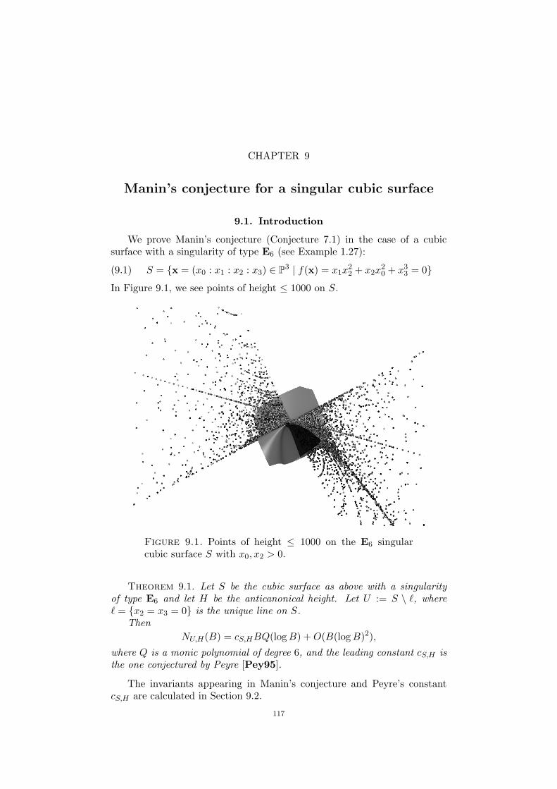
CHAPTER 9
Manin’s conjecture for a singular cubic surface
9.1. Introduction
We prove Manin’s conjecture (Conjecture 7.1) in the case of a cubicsurface with a singularity of type E6 (see Example 1.27):
(9.1) S = {x = (x0 : x1 : x2 : x3) ∈ P3 | f(x) = x1x22 + x2x
20 + x3
3 = 0}
In Figure 9.1, we see points of height ≤ 1000 on S.
Figure 9.1. Points of height ≤ 1000 on the E6 singularcubic surface S with x0, x2 > 0.
Theorem 9.1. Let S be the cubic surface as above with a singularityof type E6 and let H be the anticanonical height. Let U := S \ `, where` = {x2 = x3 = 0} is the unique line on S.
ThenNU,H(B) = cS,HBQ(logB) +O(B(logB)2),
where Q is a monic polynomial of degree 6, and the leading constant cS,H isthe one conjectured by Peyre [Pey95].
The invariants appearing in Manin’s conjecture and Peyre’s constantcS,H are calculated in Section 9.2.
117

118 9. MANIN’S CONJECTURE FOR A SINGULAR CUBIC SURFACE
The proof follows the strategy of de la Breteche and Browning [BB04]and uses the universal torsor. For our particular surface, the universal torsorhas been calculated by Hassett and Tschinkel using the Cox ring; the torsoris a hypersurface in the 10-dimensional affine space [HT04]. In additionto the equation defining the torsor we need to derive certain coprimalityconditions between the coordinates. In Section 9.3 we compute the torsorand determine these conditions following the more direct approach of Heath-Brown, Browning and de la Breteche [HB03], [Bro04], [BB04].
The next step is to count the number of integral points on the univer-sal torsor and satisfying the coprimality conditions and subject to certainbounds, given by lifting the height function to the torsor. For three of theten variables on the torsor, this summation is done in Section 9.5 by ele-mentary methods from analytic number theory. The summation over thelast seven variables, completing the proof of Theorem 9.1, is carried out inSection 9.6.
The results of this chapter first appeared in [Der05]. Section 7.3 dis-cusses joint work with de la Breteche and Browning which proves a versionof Theorem 9.1 with an improved error term, to appear in [BBD05].
9.2. Manin’s conjecture
In this section, we calculate the invariants appearing in Manin’s conjec-ture and its refinement by Peyre. We use the notation from [Pey95].
Lemma 9.2. Manin’s conjecture predicts in case of S as defined in (9.1):
NU,H(B) ∼ cS,HB(logB)6,
where cS,H = α(S)β(S)ωH(S) with
α(S) :=1
6!∏
i λi=
16! · 2 · 3 · 4 · 3 · 4 · 5 · 6
=1
6220800,
β(S) := 1,
ωH(S) := ω∞ · ω0,
and
λ = (λ1, λ2, λ3, λ`, λ4, λ5, λ6) := (2, 3, 4, 3, 4, 5, 6),
ω∞ := 6∫ ∫ ∫
{(t,u,v)∈R3| |tv3|≤1, |t2+u3|≤1, 0≤v≤1, |uv4|≤1}1dtdudv,
ω0 :=∏p
(1− 1
p
)7(1 +
7p
+1p2
).
Proof. By Theorem 8.5, α(S) = α′/#W , where α′ = 1/120 is theconstant associated to smooth split cubic surfaces, and #W = 51840 is theorder of the Weyl group W associated to the root system E6.
The surface S is split over Q, so that
β(S) = #H1(Q,Pic(S)) = 1.

9.3. THE UNIVERSAL TORSOR 119
By definition,
ωH(S) = lims→1
((s− 1)rkPic(eS)L(s,Pic(S)))ω∞(S)∏p
ωp(S)
Lp(1,Pic(S)),
where, in our case,
lims→1
((s− 1)rkPic(eS)L(s,Pic(S))) = lims→1
((s− 1)7ζ(s)7) = 1
andLp(1,Pic(S))−1 = (1− 1/p)7.
We use Peyre’s method [Pey95] to compute ω∞(S) and parameterizethe points by writing x1 as a function of x0, x2, x3. Since x = −x in P3, wemay assume x2 ≥ 0. Since d
dx1f = x2
2, the Leray form ωL(S) is given byx−2
2 dx0dx3dx2, and we obtain ω∞(S) from∫ ∫ ∫{|x0|≤1, |x−2
2 (x2x20+x3
3)|≤1, 0≤x2≤1, |x3|≤1}x−2
2 dx0dx3dx2,
using the transformations
x0 = tx1/22 , x3 = ux
2/32 , x2 = v6.
The calculation of
ωp(S) = 1 +7p
+1p2
is done as in [BB04, Lemma 1], and we omit it here. �
9.3. The universal torsor
The universal torsor
TeS = Spec(Q[ξ1, ξ2, ξ3, ξ`, ξ4, ξ5, ξ6, τ1, τ2, τ`]/(T (ξi, τi)))
is given by the equation
(9.2) T (ξi, τi) = τ`ξ3` ξ
24ξ5 + τ2
2 ξ2 + τ31 ξ
21ξ3 = 0
and the map Ψ : TeS → S = Spec(Q[x0, . . . , x3]/(f(x))) defined by
Ψ∗(x0) = ξ(1,2,2,0,1,2,3)τ2
Ψ∗(x1) = τ`
Ψ∗(x2) = ξ(2,3,4,3,4,5,6)
Ψ∗(x3) = ξ(2,2,3,1,2,3,4)τ1
(9.3)
where we use the notation ξ(n1,n2,n3,n`,n4,n5,n6) := ξn11 ξn2
2 ξn33 ξn`
` ξn44 ξn5
5 ξn66 .
Note that Ψ∗(x2) = ξλ with λ ∈ Z7 as in Lemma 9.2.We establish a bijection between rational points on the surface S and
integral points on the torsor TeS which are subject to certain coprimalityconditions. More precisely, the coprimality conditions can be summarized inthe following table, where a “−” means that the two variables are coprime,and a “×” that they may have common factors. For a variable combinedwith itself, “−” means that each prime occurs at most once (which can be
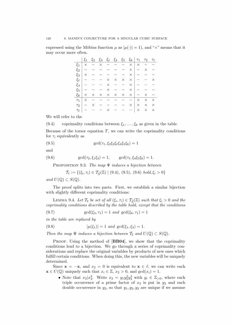
120 9. MANIN’S CONJECTURE FOR A SINGULAR CUBIC SURFACE
expressed using the Mobius function µ as |µ(·)| = 1), and “×” means that itmay occur more often.
ξ1 ξ2 ξ3 ξ` ξ4 ξ5 ξ6 τ1 τ2 τ`ξ1 × − × − − − × × − −ξ2 − − − − − − × − × −ξ3 × − − − − − × − − −ξ` − − − × × × × − − ×ξ4 − − − × − − × − − −ξ5 − − − × − − × − − −ξ6 × × × × × × × − × −τ1 × − − − − − − × × ×τ2 − × − − − − × × × ×τ` − − − × − − − × × ×
We will refer to the
(9.4) coprimality conditions between ξ1, . . . , ξ6 as given in the table.
Because of the torsor equation T , we can write the coprimality conditionsfor τi equivalently as
(9.5) gcd(τ1, ξ2ξ3ξ`ξ4ξ5ξ6) = 1
and
(9.6) gcd(τ2, ξ1ξ3) = 1, gcd(τ`, ξ4ξ5ξ6) = 1.
Proposition 9.3. The map Ψ induces a bijection between
T1 := {(ξi, τi) ∈ TeS(Z) | (9.4), (9.5), (9.6) hold, ξi > 0}
and U(Q) ⊂ S(Q).
The proof splits into two parts. First, we establish a similar bijectionwith slightly different coprimality conditions:
Lemma 9.4. Let T2 be set of all (ξi, τi) ∈ TeS(Z) such that ξi > 0 and thecoprimality conditions described by the table hold, except that the conditions
(9.7) gcd(ξ3, τ1) = 1 and gcd(ξ6, τ1) = 1
in the table are replaced by
(9.8) |µ(ξ1)| = 1 and gcd(ξ1, ξ3) = 1.
Then the map Ψ induces a bijection between T2 and U(Q) ⊂ S(Q).
Proof. Using the method of [BB04], we show that the coprimalityconditions lead to a bijection. We go through a series of coprimality con-siderations and replace the original variables by products of new ones whichfulfill certain conditions. When doing this, the new variables will be uniquelydetermined.
Since x = −x, and x2 = 0 is equivalent to x ∈ `, we can write eachx ∈ U(Q) uniquely such that xi ∈ Z, x2 > 0, and gcd(xi) = 1.
• Note that x2|x33. Write x2 = y1y
22y
33 with yi ∈ Z>0, where each
triple occurrence of a prime factor of x3 is put in y3 and eachdouble occurrence in y2, so that y1, y2, y3 are unique if we assume
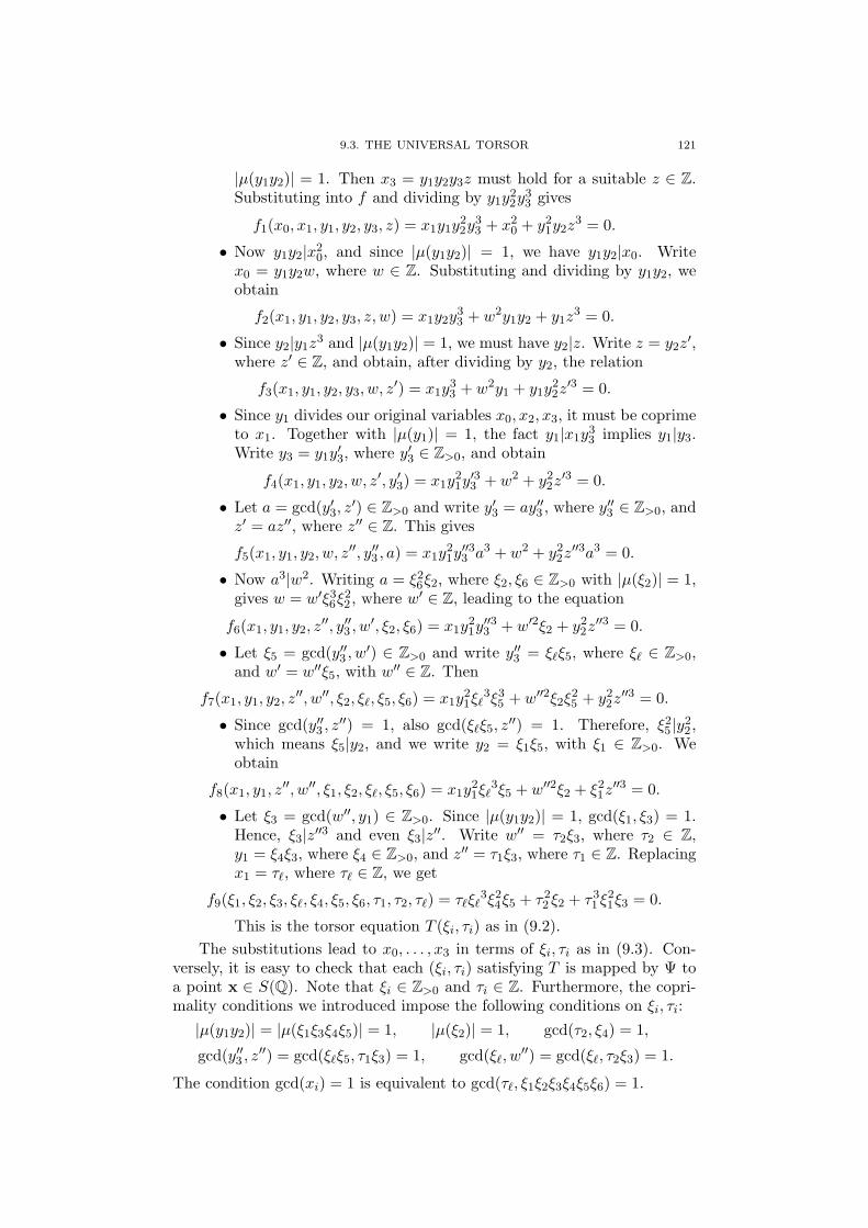
9.3. THE UNIVERSAL TORSOR 121
|µ(y1y2)| = 1. Then x3 = y1y2y3z must hold for a suitable z ∈ Z.Substituting into f and dividing by y1y
22y
33 gives
f1(x0, x1, y1, y2, y3, z) = x1y1y22y
33 + x2
0 + y21y2z
3 = 0.
• Now y1y2|x20, and since |µ(y1y2)| = 1, we have y1y2|x0. Write
x0 = y1y2w, where w ∈ Z. Substituting and dividing by y1y2, weobtain
f2(x1, y1, y2, y3, z, w) = x1y2y33 + w2y1y2 + y1z
3 = 0.
• Since y2|y1z3 and |µ(y1y2)| = 1, we must have y2|z. Write z = y2z
′,where z′ ∈ Z, and obtain, after dividing by y2, the relation
f3(x1, y1, y2, y3, w, z′) = x1y
33 + w2y1 + y1y
22z′3 = 0.
• Since y1 divides our original variables x0, x2, x3, it must be coprimeto x1. Together with |µ(y1)| = 1, the fact y1|x1y
33 implies y1|y3.
Write y3 = y1y′3, where y′3 ∈ Z>0, and obtain
f4(x1, y1, y2, w, z′, y′3) = x1y
21y
′33 + w2 + y2
2z′3 = 0.
• Let a = gcd(y′3, z′) ∈ Z>0 and write y′3 = ay′′3 , where y′′3 ∈ Z>0, and
z′ = az′′, where z′′ ∈ Z. This gives
f5(x1, y1, y2, w, z′′, y′′3 , a) = x1y
21y
′′33 a3 + w2 + y2
2z′′3a3 = 0.
• Now a3|w2. Writing a = ξ26ξ2, where ξ2, ξ6 ∈ Z>0 with |µ(ξ2)| = 1,gives w = w′ξ36ξ
22 , where w′ ∈ Z, leading to the equation
f6(x1, y1, y2, z′′, y′′3 , w
′, ξ2, ξ6) = x1y21y
′′33 + w′2ξ2 + y2
2z′′3 = 0.
• Let ξ5 = gcd(y′′3 , w′) ∈ Z>0 and write y′′3 = ξ`ξ5, where ξ` ∈ Z>0,
and w′ = w′′ξ5, with w′′ ∈ Z. Then
f7(x1, y1, y2, z′′, w′′, ξ2, ξ`, ξ5, ξ6) = x1y
21ξ`
3ξ35 + w′′2ξ2ξ25 + y2
2z′′3 = 0.
• Since gcd(y′′3 , z′′) = 1, also gcd(ξ`ξ5, z′′) = 1. Therefore, ξ25 |y2
2,which means ξ5|y2, and we write y2 = ξ1ξ5, with ξ1 ∈ Z>0. Weobtain
f8(x1, y1, z′′, w′′, ξ1, ξ2, ξ`, ξ5, ξ6) = x1y
21ξ`
3ξ5 + w′′2ξ2 + ξ21z′′3 = 0.
• Let ξ3 = gcd(w′′, y1) ∈ Z>0. Since |µ(y1y2)| = 1, gcd(ξ1, ξ3) = 1.Hence, ξ3|z′′3 and even ξ3|z′′. Write w′′ = τ2ξ3, where τ2 ∈ Z,y1 = ξ4ξ3, where ξ4 ∈ Z>0, and z′′ = τ1ξ3, where τ1 ∈ Z. Replacingx1 = τ`, where τ` ∈ Z, we get
f9(ξ1, ξ2, ξ3, ξ`, ξ4, ξ5, ξ6, τ1, τ2, τ`) = τ`ξ`3ξ24ξ5 + τ2
2 ξ2 + τ31 ξ
21ξ3 = 0.
This is the torsor equation T (ξi, τi) as in (9.2).The substitutions lead to x0, . . . , x3 in terms of ξi, τi as in (9.3). Con-
versely, it is easy to check that each (ξi, τi) satisfying T is mapped by Ψ toa point x ∈ S(Q). Note that ξi ∈ Z>0 and τi ∈ Z. Furthermore, the copri-mality conditions we introduced impose the following conditions on ξi, τi:
|µ(y1y2)| = |µ(ξ1ξ3ξ4ξ5)| = 1, |µ(ξ2)| = 1, gcd(τ2, ξ4) = 1,
gcd(y′′3 , z′′) = gcd(ξ`ξ5, τ1ξ3) = 1, gcd(ξ`, w′′) = gcd(ξ`, τ2ξ3) = 1.
The condition gcd(xi) = 1 is equivalent to gcd(τ`, ξ1ξ2ξ3ξ4ξ5ξ6) = 1.
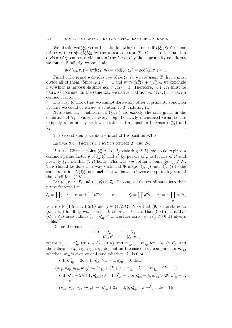
122 9. MANIN’S CONJECTURE FOR A SINGULAR CUBIC SURFACE
We obtain gcd(ξ2, ξ3) = 1 in the following manner: If p|ξ2, ξ3 for someprime p, then p|τ`ξ3` ξ24ξ5 by the torsor equation T . On the other hand, adivisor of ξ3 cannot divide any of the factors by the coprimality conditionswe found. Similarly, we conclude
gcd(ξ3, τ2) = gcd(ξ1, τ2) = gcd(ξ2, ξ5) = gcd(ξ5, τ2) = 1.
Finally, if a prime p divides two of ξ2, ξ4, τ1, we see using T that p mustdivide all of them. Since |µ(ξ2)| = 1 and p2|τ`ξ3` ξ24ξ5 + τ3
1 ξ21ξ3, we conclude
p|τ2 which is impossible since gcd(τ2, ξ4) = 1. Therefore, ξ2, ξ4, τ1 must bepairwise coprime. In the same way we derive that no two of ξ1, ξ2, ξ` have acommon factor.
It is easy to check that we cannot derive any other coprimality conditionbecause we could construct a solution to T violating it.
Note that the conditions on (ξi, τi) are exactly the ones given in thedefinition of T2. Since in every step the newly introduced variables areuniquely determined, we have established a bijection between U(Q) andT2. �
The second step towards the proof of Proposition 9.3 is:
Lemma 9.5. There is a bijection between T1 and T2.
Proof. Given a point (ξ′i, τ′j) ∈ T2 violating (9.7), we could replace a
common prime factor p of ξ′3, ξ′6 and τ ′1 by powers of p as factors of ξ′1 and
possibly ξ′3 such that (9.7) holds. This way, we obtain a point (ξi, τj) ∈ T1.This should be done in a way such that Ψ maps (ξi, τj) and (ξ′i, τ
′j) to the
same point x ∈ U(Q), and such that we have an inverse map, taking care ofthe conditions (9.8).
Let (ξi, τj) ∈ T1 and (ξ′i, τ′j) ∈ T2. Decompose the coordinates into their
prime factors: Let
ξi =∏p
pnip , τj = ±∏p
pmjp and ξ′i =∏p
pn′ip , τ ′j = ±∏p
pm′jp ,
where i ∈ {1, 2, 3, `, 4, 5, 6} and j ∈ {1, 2, `}. Note that (9.7) translates to(nip,mjp) fulfilling n3p = n6p = 0 or m1p = 0, and that (9.8) means that(n′ip,m
′jp) must fulfill n′1p + n′3p ≤ 1. Furthermore, n3p, n
′3p ∈ {0, 1} always
holds.Define the map
Φ′ : T2 → T1
(ξ′i, τ′i) 7→ (ξi, τj),
where nip := n′ip for i ∈ {2, `, 4, 5} and mjp := m′jp for j ∈ {2, `}, and
the values of n1p, n3p, n6p,m1p depend on the size of n′6p compared to m′1p,
whether m′1p is even or odd, and whether n′3p is 0 or 1:
• If m′1p = 2k + 1, n′6p ≥ k + 1, n′3p = 0, then
(n1p, n3p, n6p,m1p) := (n′1p + 3k + 1, 1, n′6p − k − 1,m′1p − 2k − 1);
• if m′1p = 2k+ 1, n′6p ≥ k+ 1, n′3p = 1 or n′6p = k,m′
1p > 2k, n′3p = 1,then
(n1p, n3p, n6p,m1p) := (n′1p + 3k + 2, 0, n′6p − k,m′1p − 2k − 1);

9.4. CONGRUENCES 123
• otherwise, with n′6p = k,m′1p > 2k, n′3p = 0 or m′
1p = 2k, n′6p ≥ k:
(n1p, n3p, n6p,m1p) := (n′1p + 3k, n′3p, n′6p − k,m′
1p − 2k).
Conversely, defineΦ : T1 → T2
(ξi, τi) 7→ (ξ′i, τ′j),
where n′ip := nip for i ∈ {2, `, 4, 5} and m′jp := mjp for j ∈ {2, `}, and the
values of n′1p, n′3p, n
′6p,m
′1p depend on n1p modulo 3 and whether n3p is 0 or
1:• If n1p ∈ {3k + 1, 3k + 2} and n3p = 1, then
(n′1p, n′3p, n
′6p,m
′1p) := (n1p − 3k − 1, 0, n6p + k + 1,m1p + 2k + 1);
• if n1p = 3k + 2 and n3p = 0, then
(n′1p, n′3p, n
′6p,m
′1p) := (n1p − 3k − 2, 1, n6p + k,m1p + 2k + 1);
• otherwise, with n1p ∈ {3k, 3k + 1}:
(n′1p, n′3p, n
′6p,m
′1p) := (n1p − 3k, n3p, n6p + k,m1p + 2k).
It is not difficult to check that Φ and Φ′ are well-defined, that (ξi, τj) ∈ TeS(Z)and (ξ′i, τ
′j) ∈ TeS(Z) correspond to the same point x ∈ U(Q) under the map
Ψ, and that Φ and Φ′ are inverse to each other. �
Together, Lemma 9.4 and Lemma 9.5 prove Proposition 9.3.
9.4. Congruences
We use the following results from [BB04, Chapter 3] on the number ofsolutions of linear and quadratic congruences.
Let η(a; q) be the number of positive integers n ≤ q such that n2 ≡a (mod q). Then by [BB04, Equation 3.1], we have for any q ∈ Z>0
(9.9) η(a; q) ≤ 2ω(q),
where ω(q) is the number of distinct prime factors of q. Let ϑ be an arith-metic function such that
∞∑d=1
|(ϑ ∗ µ)(d)| <∞,
where ϑ ∗ µ is the usual Dirichlet convolution.
Lemma 9.6. Let a, q ∈ Z such that q > 0 and gcd(a, q) = 1. For t ≥ 0,∑n≤t
n≡a (mod q)
ϑ(n) =t
q
∞∑d=1
gcd(d,q)=1
(ϑ ∗ µ)(d) +O
( ∞∑d=1
|(ϑ ∗ µ)(d)|
).
Proof. This is the case κ = 0 of [BB04, Lemma 2]. �
Let ψ(t) = {t} − 1/2 where {t} is the fractional part of t ∈ R. Letψ(t) = ψ(t) + 1 for t ∈ Z and ψ(t) = ψ(t) otherwise.
124 9. MANIN’S CONJECTURE FOR A SINGULAR CUBIC SURFACE
Lemma 9.7. Let a, q ∈ Z, where q > 0 and gcd(a, q) = 1. Let b1, b2 ∈ Rwith b1 ≤ b2. Then
#{n | b1 ≤ n ≤ b2, n ≡ a (mod q)} =b2 − b1q
+ r(b1, b2; a, q),
where
r(b1, b2; a, q) = ψ
(b1 − a
q
)− ψ
(b2 − a
q
).
Proof. This is a slight generalization of [BB04, Lemma 3]. �
Lemma 9.8. Let ε > 0 and t ≥ 0. Let a, q ∈ Z such that q > 0 andgcd(a, q) = 1. Then∑
0≤%<qgcd(%,q)=1
ψ
(t− a%2
q
)�εq
1/2+ε and∑
0≤%<qgcd(%,q)=1
ψ
(t− a%2
q
)�εq
1/2+ε.
Proof. For ψ, this is [BB04, Lemma 5].Note that if t ≡ a%2
i (mod q) for i ∈ {1, 2}, then %1 ≡ ±%2 (mod q), whichimplies that there are at most two different values for % with 0 ≤ % < q suchthat (t − a%2)/q is integral. Consequently, the sum for ψ differs from theone for ψ at most by 2. �
9.5. Summations
Note that τ` is determined uniquely by T and the other variables, oncea certain congruence is fulfilled. Therefore, our strategy is first to computethe number of possible τ2 depending on τ1, ξi such that there exists a uniqueτ` satisfying T . By summing over τ1, the number of possible τi is thencomputed depending on ξi. The summation over the variables ξi is finallyhandled using the height zeta function.
Let
X1 = (Bξ(−2,0,−1,3,2,1,0))1/3, X2 = (Bξ(0,−1,0,3,2,1,0))1/2,
andX0 = (B−1ξ(2,3,4,3,4,5,6))1/6.
Then the height conditions |xi| ≤ B lift to
(9.10)∣∣∣∣( τ2X2
)X3
0
∣∣∣∣ ≤ 1,
∣∣∣∣∣(τ2X2
)2
+(τ1X1
)3∣∣∣∣∣ ≤ 1,
and
(9.11) |X0| ≤ 1,
and
(9.12)∣∣∣∣( τ1X1
)X4
0
∣∣∣∣ ≤ 1,
respectively.Using Proposition 9.3, we can now relate the counting of rational points
of bounded height on U ⊂ S to a count on the torsor.

9.5. SUMMATIONS 125
Lemma 9.9. We have
NU,H(B) = #
{(ξi, τi) ∈ TeS(Z)
∣∣∣∣∣ (9.4), (9.5), (9.6),
(9.10), (9.11), (9.12) hold, ξi > 0
}.
Summation over τ2 and τ`. Let ξi, τ1 satisfy the coprimality conditions(9.4), (9.5) and the height conditions (9.11) and (9.12). Let N = N(ξi, τ1)be the number of pairs (τ2, τ`) such that (9.6), (9.10) and the torsor equationT are fulfilled. Then a Mobius inversion gives
N =∑
k`|ξ4ξ5ξ6
µ(k`)Nk`,
where Nk`has the same definition as N except that gcd(τ`, ξ4ξ5ξ6) = 1 is
removed, and T is replaced by
Tk`(ξi, τi, k`) = k`τ`ξ
3` ξ
24ξ5 + τ2
2 ξ2 + τ31 ξ
21ξ3 = 0.
Note that τ2 together with Tk`defines τ` uniquely once a certain congruence
is fulfilled. Therefore,
Nk`= #
{τ2
∣∣∣∣∣ gcd(τ2, ξ1ξ3) = 1, (9.10) holds,
−τ22 ξ2 ≡ τ3
1 ξ21ξ3 (mod k`ξ
3` ξ
24ξ5)
}.
Note that
gcd(τ31 ξ
21ξ3, k`ξ
3` ξ
24ξ5) = gcd(τ3
1 ξ21ξ3, ξ4ξ5ξ6, τ
22 ξ2) = gcd(τ1, ξ6, τ2
2 ξ2) = 1
and
gcd(ξ2, k`ξ3` ξ
24ξ5) = gcd(ξ2, k`) = gcd(ξ2, ξ4ξ5ξ6, τ3
1 ξ21ξ3) = 1.
Hence, it is enough to sum over all k`|ξ4ξ5ξ6 with gcd(k`, τ1ξ1ξ2ξ3) = 1,and since k`|ξ4ξ5ξ6 implies gcd(k`, τ1) = 1, we reduce to gcd(k`, ξ1ξ2ξ3) = 1.
This implies that there is a unique integer % satisfying 0 < % ≤ k`ξ3` ξ
24ξ5
and gcd(%, k`ξ3` ξ
24ξ5) = 1 such that
τ2 ≡ %τ1ξ1 (mod k`ξ3` ξ
24ξ5) and −%2ξ2 ≡ τ1ξ3 (mod k`ξ
3` ξ
24ξ5).
We have
N =∑
k`|ξ4ξ5ξ6gcd(k`,ξ1ξ2ξ3)=1
µ(k`)∑
0<%≤k`ξ3` ξ2
4ξ5−%2ξ2≡τ1ξ3 (mod k`ξ
3` ξ2
4ξ5)
gcd(%,k`ξ3` ξ2
4ξ5)=1
Nk`(%)
where
Nk`(%) = #
{τ2
∣∣∣∣∣ gcd(τ2, ξ1ξ3) = 1, (9.10) holds,
τ2 ≡ %τ1ξ1 (mod k`ξ3` ξ
24ξ5)
}.
We also know that gcd(%τ1ξ1, k`ξ3` ξ
24ξ5) = 1. Now we can apply Lemma 9.6
to the characteristic function
χ(n) =
{1, if gcd(n, ξ1ξ3) = 1,0, else.

126 9. MANIN’S CONJECTURE FOR A SINGULAR CUBIC SURFACE
Since∞∑
d=1gcd(d,k`ξ
3` ξ2
4ξ5)=1
(χ ∗ µ)(d)d
=∏
p|ξ1ξ3p-k`ξ
3` ξ2
4ξ5
(1− 1
p
)=∏
p|ξ1ξ3
(1− 1
p
)= φ∗(ξ1ξ3),
where we use gcd(ξ1ξ3, k`ξ3` ξ
24ξ5) = 1 and the notation φ∗(n) := φ(n)/n as
in [BB04, Equation 5.10], we conclude
Nk`(%) =
φ∗(ξ1ξ3)X2
k`ξ3` ξ
24ξ5
g1(τ1/X1, X0) +O(2ω(ξ1ξ3)),
where X2g1(τ1/X1, X0) gives the total length of the intervals in which τ2must lie by (9.10), with
(9.13) g1(u, v) =∫{t∈R| |tv3|≤1, |t2+u3|≤1}
1dt.
By equation (9.9), the number of integers % with 0 < % ≤ k`ξ3` ξ
24ξ5 such
that gcd(%, k`ξ3` ξ
24ξ5) = 1 and −%2ξ2 ≡ τ1ξ3 (mod k`ξ
3` ξ
24ξ5) is at most
η(ξ2ξ3τ1; k`ξ3` ξ
24ξ5) ≤ 2ω(k`ξ
3` ξ2
4ξ5) ≤ 2ω(ξ`ξ4ξ5ξ6).
This gives as the first step towards the proof of Theorem 9.1:
Lemma 9.10.
N =X2
ξ3` ξ24ξ5
g1(τ1/X1, X0)Σ(ξi, τ1) +O(2ω(ξ1ξ3)+ω(ξ`ξ4ξ5ξ6)+ω(ξ4ξ5ξ6)),
where
Σ(ξi, τ1) = φ∗(ξ1ξ3)∑
k`|ξ4ξ5ξ6gcd(k`,ξ1ξ2ξ3)=1
µ(k`)k`
∑0<%≤k`ξ
3` ξ2
4ξ5−%2ξ2≡τ1ξ3 (mod k`ξ
3` ξ2
4ξ5)
gcd(%,k`ξ3` ξ2
4ξ5)=1
1.
Now we show that the error term suffices for Theorem 9.1: We sum itover all the ξi, τ1 which satisfy the height conditions (9.11) and (9.12); wecan ignore the coprimality conditions (9.4), (9.5), (9.6). We obtain:∑
ξi
∑τ1
2ω(ξ1ξ3)+ω(ξ`ξ4ξ5ξ6)+ω(ξ4ξ5ξ6)
�∑ξi
2ω(ξ1ξ3)+ω(ξ`ξ4ξ5ξ6)+ω(ξ4ξ5ξ6)X1
X40
=∑ξi
2ω(ξ1ξ3)+ω(ξ`ξ4ξ5ξ6)+ω(ξ4ξ5ξ6) B
ξ(2,2,3,1,2,3,4)
�B(logB)2∑
ξi,i6=`
2ω(ξ1ξ3)+ω(ξ4ξ5ξ6)+ω(ξ4ξ5ξ6)
ξ(2,2,3,0,2,3,4)
�B(logB)2.
For ξ`, we have used the estimate∑n≤x
2ω(n) � x(log x)

9.5. SUMMATIONS 127
together with partial summation.Therefore, we only need to consider the main term when summing over
τ1, ξi in order to prove Theorem 9.1.
Summation over τ1. For fixed ξ1, . . . , ξ6 satisfying (9.4) and (9.11), wesum over all τ1 satisfying the coprimality condition (9.5) and the heightcondition (9.12). Let
N ′ = N ′(ξi) =X2
ξ3` ξ24ξ5
∑τ1, (9.12) holds
gcd(τ1,ξ2ξ3ξ`ξ4ξ5ξ6)=1
g1(τ1/X1, X0)Σ(ξi, τ1).
First, we find an asymptotic formula for
N (b1, b2) = φ∗(ξ1ξ3)∑
k`|ξ4ξ5ξ6gcd(k`,ξ1ξ2ξ3)=1
µ(k`)k`
∑0<%≤k`ξ
3` ξ2
4ξ5gcd(%,k`ξ
3` ξ2
4ξ5)=1
N ′k`
(%, b1, b2),
where
N ′k`
(%, b1, b2) = #
{τ1 ∈ [b1, b2]
∣∣∣∣ gcd(τ1, ξ2ξ3ξ`ξ4ξ5ξ6) = 1,
−%2ξ2 ≡ τ1ξ3 (mod k`ξ3` ξ
24ξ5)
}.
We have gcd(%2ξ2, k`ξ3` ξ
24ξ5) = 1. Hence, we can replace the condi-
tion gcd(τ1, ξ2ξ3ξ`ξ4ξ5ξ6) = 1 by gcd(τ1, ξ2ξ3ξ6) = 1 in the definition ofN ′
k`(%, b1, b2) and perform another Mobius inversion to obtain
N (b1, b2) =φ∗(ξ1ξ3)∑
k`|ξ4ξ5ξ6gcd(k`,ξ1ξ2ξ3)=1
µ(k`)k`
∑k1|ξ2ξ3ξ6
gcd(k1,k`ξ3` ξ2
4ξ5)=1
µ(k1)
∑0<%≤k`ξ
3` ξ2
4ξ5gcd(%,k`ξ
3` ξ2
4ξ5)=1
N ′k`,k1
(%, b1, b2),
where
N ′k`,k1
(%, b1, b2) = #{τ1 ∈ [b1/k1, b2/k1] | −%2ξ2 ≡ k1τ1ξ3 (mod k`ξ3` ξ
24ξ5)}.
Note that we must only sum over the k1 with gcd(k1, k`ξ3` ξ
24ξ5) because of
gcd(%2ξ2, k`ξ3` ξ
24ξ5) = 1.
Let a = a(ξi, k1, k`) be the unique integer such that 0 < a ≤ k`ξ3` ξ
24ξ5
and−ξ2 ≡ k1aξ3 (mod k`ξ
3` ξ
24ξ5).
Then −%2ξ2 ≡ k1τ1ξ3 (mod k`ξ3` ξ
24ξ5) if and only if τ1 ≡ a%2 (mod k`ξ
3` ξ
24ξ5).
Since gcd(ξ2, k`ξ3` ξ
24ξ5) = 1, we have gcd(a, k`ξ
3` ξ
24ξ5) = 1. By Lemma 9.7,
we conclude
N ′k`,k1
(%, b1, b2) =b2 − b1
k1k`ξ3` ξ
24ξ5
+ r(b1/k1, b2/k1, a%2, k`ξ
3` ξ
24ξ5)
where, by definition of r,
r(b1/k1, b2/k1, a%2, k`ξ
3` ξ
24ξ5) = ψ
(b1/k1 − a%2
k`ξ3` ξ
24ξ5
)− ψ
(b2/k1 − a%2
k`ξ3` ξ
24ξ5
).

128 9. MANIN’S CONJECTURE FOR A SINGULAR CUBIC SURFACE
Let
ϑ = ϑ(ξi) =
{φ∗(ξ1ξ3)φ∗(ξ2ξ3ξ`ξ4ξ5ξ6)
φ∗(ξ4ξ5ξ6)φ∗(gcd(ξ4ξ5ξ6,ξ1ξ2ξ3)) , (9.4) holds,
0, otherwise.
Then for any b1 < b2, we have
N (b1, b2) = ϑ(ξ) · (b2 − b1) +R(b1, b2)
where
R(b1, b2) =φ∗(ξ1ξ3)∑
k`|ξ4ξ5ξ6gcd(τ`,ξ4ξ5ξ6)=1
µ(k`)k`
∑k1|ξ2ξ3ξ6
gcd(k1,k`ξ3` ξ2
4ξ5)=1
µ(k1)
∑0<%≤k`ξ
3` ξ2
4ξ5gcd(%,k`ξ
3` ξ2
4ξ5)=1
r(b1/k1, b2/k1, a%2, k`ξ
3` ξ
24ξ5).
By partial summation, we obtain
N ′(ξi) =ϑ(ξi)X1X2
ξ3` ξ24ξ5
g2(X0) +R′(ξi)
with
(9.14) g2(v) =∫{u∈R| |uv4|≤1}
g1(u, v)du
and
R′(ξi) =−X2
ξ3` ξ24ξ5
∫ X−40
−X−40
(D1g1)(u,X0)R(−X1/X40 , X1u)du
where D1g1 is the derivation of g1 with respect to the first variable.
Lemma 9.11. For any ξi as in (9.4), (9.11), we have
N ′(ξi) =ϑ(ξi)X1X2
ξ3` ξ24ξ5
g2(X0) +R′(ξi)
where the error term R′(ξi) satisfies∑ξi, (9.4), (9.11) holds
R′(ξi) = O(B logB).
Proof. By Lemma 9.8, we have
R(b1, b2)�εφ∗(ξ1ξ3)
∑k`|ξ4ξ5ξ6
gcd(τ`,ξ4ξ5ξ6)=1
|µ(k`)|k`
∑k1|ξ2ξ3ξ6
gcd(k1,k`ξ3` ξ2
4ξ5)=1
|µ(k1)|(k`ξ3` ξ
24ξ5)
1/2+ε
≤∑
k`|ξ4ξ5ξ6gcd(τ`,ξ4ξ5ξ6)=1
|µ(k`)|∑
k1|ξ2ξ3ξ6gcd(k1,k`ξ
3` ξ2
4ξ5)=1
|µ(k1)|(ξ3` ξ24ξ5)1/2+ε
≤ 2ω(ξ4ξ5ξ6)+ω(ξ2ξ3ξ6)(ξ3` ξ24ξ5)
1/2+ε.
9.6. COMPLETION OF THE PROOF 129
Therefore,
R′(ξi)�εX2
ξ3` ξ24ξ5
∫ X−40
−X−40
(D1g1)(u,X0)2ω(ξ4ξ5ξ6)+ω(ξ2ξ3ξ6)(ξ3` ξ24ξ5)
1/2+εdu
� X2
(ξ3` ξ24ξ5)1/2−ε
2ω(ξ4ξ5ξ6)+ω(ξ2ξ3ξ6).
Summing this over all ξi ≤ B, we get, using (9.11),∑ξi≤B
(9.4), (9.11) hold
R′(ξi)�ε
∑ξi≤B
X2
X30 (ξ3` ξ
24ξ5)1/2−ε
2ω(ξ4ξ5ξ6)+ω(ξ2ξ3ξ6)
=∑ξi≤B
B
ξ(1,2,2,3/2−3ε,2−2ε,5/2−ε,3)2ω(ξ4ξ5ξ6)+ω(ξ2ξ3ξ6)
�∑
ξi,i6=1
B logBξ(0,2,2,3/2−3ε,2−2ε,5/2−ε,3)
2ω(ξ4ξ5ξ6)+ω(ξ2ξ3ξ6)
� B logB.
�
Summation over ξi. Define
∆(n) = B−5/6∑
ξi,ξ(2,3,4,3,4,5,6)=n
ϑ(ξi)X1X2
ξ3` ξ24ξ5
.
We sum N ′(ξi) in Lemma 9.11 over the seven variables ξi such that thecoprimality conditions (9.4) and the height condition (9.11) hold. Note thatthe definition of ϑ(ξi) ensures that the main term of N ′(ξi) is zero if (9.4)is not satisfied. In view of Lemma 9.9, this implies:
Lemma 9.12. We have
NU,H(B) = B5/6∑n≤B
∆(n)g2((n/B)1/6) +O(B(logB)2).
9.6. Completion of the proof
Our argument is similar to [BB04]. We need to estimate
M(t) :=∑n≤t
∆(n)
for t > 1. Therefore, we consider the Dirichlet series F (s) :=∑∞
n=1 ∆(n)n−s.Observing
X1X2
ξ3` ξ24ξ5
=B5/6(ξ(2,3,4,3,4,5,6))1/6
ξ(1,1,1,1,1,1,1),
we get
F (s+ 1/6) =∑ξi
ϑ(ξi)ξ2s+11 ξ3s+1
2 ξ4s+13 ξ3s+1
` ξ4s+14 ξ5s+1
5 ξ6s+16
,
130 9. MANIN’S CONJECTURE FOR A SINGULAR CUBIC SURFACE
and writing F (s + 1/6) =∏
p Fp(s + 1/6) as a product of local factors, weobtain:
Fp(s+ 1/6) =1 +(1− 1/p)2
(pλ6s+1 − 1)
(pλ1s+1
pλ1s+1 − 1+
pλ1s+1pλ6s+1
pλ3s+1(pλ1s+1 − 1)
+pλ6s+1
(1− 1/p)pλ2s+1+
1pλ`s+1 − 1
+pλ`s+1pλ6s+1
pλ4s+1(pλ`s+1 − 1)
+pλ`s+1pλ6s+1
pλ5s+1(pλ`s+1 − 1)
)+
1− 1/ppλ1s+1 − 1
+1− 1/ppλ`s+1 − 1
for any prime p.Since 1/pλis+1 = Oε(1/p1/2+ε) for s ∈ H := {s ∈ C | <e(s) ≥ −1/12+ ε}
and i ∈ {1, 2, 3, `, 4, 5, 6}, we have
Fp(s+ 1/6) = 1 +∑
i
1pλis+1
+Oε
(1
p1+ε
)for s ∈ H, and defining
E(s) :=∏
i
ζ(λis+ 1) = ζ(2s+ 1)ζ(3s+ 1)2ζ(4s+ 1)2ζ(5s+ 1)ζ(6s+ 1),
we have1
Ep(s)= 1−
∑i
1pλis+1
+Oε
(1
p1+ε
)for s ∈ H. Define
G(s) := F (s+ 1/6)/E(s)for <e(s) > 0. Then G has a holomorphic and bounded continuation to H.Note that
G(0) =∏p
(1− 1
p
)7(1 +
7p
+1p2
),
and that for s→ 0, we have
E(s) =1∏i λi
s−7 +O(s−6).
Consequently, the residue of F (s)ts/s at s = 1/6 is
Res(t) =6G(0)t1/6Q1(log t)
6! ·∏
i λi
for some monic polynomial Q1 of degree 6.
Lemma 9.13. M(t) = ω0α(S) · 6t1/6Q1(log t) +Oε(t1/6−1/24+ε).
Proof. Integrating Perron’s formula for M(t) over t, we have∫ t
0M(u)du =
12πi
∫ 1/6+ε+i∞
1/6+ε−i∞F (s)
ts+1
s(s+ 1)ds
for t > 1 and ε > 0.We apply Cauchy’s residue theorem to the rectangle with vertices
1/12 + ε− iT, 1/12 + ε+ iT, 1/6 + ε+ iT, 1/6 + ε− iT,
for some T > 1, where ε > 0 is sufficiently small.
9.6. COMPLETION OF THE PROOF 131
By the convexity bound
ζ(1 + σ + iτ)�ε|τ |−σ/3+ε
for any σ ∈ [−1/2, 0), we have
(9.15) F (1/6 + σ + iτ) � E(σ + iτ)�ε|τ |−9σ+ε
for any σ ∈ [−1/12 + ε, 0), using (∑
i λi)/3 = 9 and that G(σ + iτ) isbounded.
For the ray going down from 1/6 + ε− iT , we get∣∣∣∣∣∫ 1/6+ε−iT
1/6+ε−i∞
F (s)ts+1
s(s+ 1)ds
∣∣∣∣∣ ≤∫ T
−∞
|F (1/6 + ε+ iσ)||t7/6+ε+iσ||(1/6 + ε+ iσ)(7/6 + ε+ iσ)
dσ
� t7/6+ε
∫ T
−∞
1|σ|2
dσ
� t7/6+εT−1
where we use that F (s) is bounded for <e(s) ≥ 1/6 + ε. Integrating from1/6 + ε+ iT to 1/6 + ε+ i∞ gives the same result.
For the lower edge, we estimate∣∣∣∣∣∫ 1/6+ε−iT
1/12+ε−iT
F (s)ts+1
s(s+ 1)ds
∣∣∣∣∣ ≤∫ ε
−1/12+ε
|F (1/6 + σ − iT )||t7/6+σ−iT ||(1/6 + σ − iT )(7/6 + σ − iT )|
dσ
�εT 9/12+εt7/6+ε
T 2,
because (9.15) gives a bound for −1/12+ε ≤ σ ≤ −ε, F (s) being continuousgives a bound in an ε-neighborhood of 1/6 − iT , and the length of theintegration interval is 1/12. For the upper edge, we obtain the same bound.
For the edge on the left, we have∣∣∣∣∣∫ 1/12+ε+iT
1/12+ε−iT
F (s)ts+1
s(s+ 1)ds
∣∣∣∣∣ ≤∫ T
−T
|F (1/12 + ε+ iσ)||t13/12+ε+iσ||(1/12 + ε+ iσ)(13/12 + ε+ iσ)
dσ
�ε
∫ T
−T
|σ|9/12+εt13/12+ε
(1 + |σ|)2dσ
� t13/12+ε
since the integral over σ is bounded independently of T , and using (9.15)again.
Taking T = t, we have proved∫ t
0M(u)du =
∫ t
0Res(u)du+Oε(t13/12+ε).
But now1H
∫ t
t−HM(u)du ≤M(t) ≤ 1
H
∫ t+H
tM(u)du,
and for H ≤ t/3, both integrals are equal to
Res(t) +Oε(Ht−5/6(log t)6 +H−1t13/12+ε).

132 9. MANIN’S CONJECTURE FOR A SINGULAR CUBIC SURFACE
The proof of the Lemma is completed by choosing H = t23/24 and notingthat ω0 = G(0) and α(S) = (6!
∏i λi)−1 by the definitions of ω0 and α(S)
in Lemma 9.2. �
By partial summation we conclude∑n≤B
∆(n)g2((n/B)1/6)
= ω0α(S) · 6∫ B
0g2(u1/6/B1/6)
ddu
(u1/6Q1(log u))du+Oε(B1/6−1/24+ε)
= B1/6ω0α(S) · 6∫ 1
0g2(v)Q2(logB + 6 log v)dv +Oε(B1/6−1/24+ε)
for some monic polynomial Q2 of degree 6. Considering definitions (9.13)and (9.14), note that
ω∞ = 6∫{v∈R|0≤v≤1}
g2(v)dv.
Together with Lemma 9.12, this completes the proof of Theorem 9.1.

CHAPTER 10
Manin’s conjecture for a singular quartic surface
10.1. Introduction
In this chapter, we illustrate the torsor approach to asymptotics of ra-tional points in the case of a particular singular surface S ⊂ P4 of degree 4given by:
(10.1) x0x3 − x1x4 = x0x1 + x1x3 + x22 = 0.
This is a split Del Pezzo surface, with a singularity of type D4. The resultsfirst appeared in [DT06],
Theorem 10.1. The number of Q-rational points of anticanonical heightbounded by B on the complement U of the Q-rational lines on S (10.1)satisfies
NU,H(B) = cS,H ·B ·Q(logB) +O(B(logB)3) as B →∞,
where Q is a monic polynomial of degree 5, and
cS,H =1
34560· ω∞ ·
∏p
(1− 1/p)6(1 + 6/p+ 1/p2)
is the constant predicted by Peyre (Section 7.2), with p running through allprimes and
ω∞ = 3∫ ∫ ∫
{(t,u,v)∈R3| 0≤v≤1, |tv2|,|v2u|,|v(tv+u2)|,|t(tv+u2)|≤1}1dtdudv.
In [BB05], Manin’s conjecture is proved for a non-split surface with asingularity of the same type. However, these results do not follow from eachother.
In Section 10.2, we collect some facts about the geometric structure ofS. In Section 10.3, we calculate the expected value of cS,H and show thatTheorem 10.1 agrees with Manin’s conjecture.
In our case, the universal torsor is an affine hypersurface. In Section 10.4,we calculate its equation, stressing the relation with the geometry of S. Wemake explicit the coprimality and the height conditions. The method ismore systematic than the derivation of the torsor equations in Chapter 9,[BB04], and [BBD05], and should generalize to more complicated cases,e.g., other split Del Pezzo surfaces.
Note that our method gives coprimality conditions which are differentfrom the ones in Chapter 9, [BB04], and [BBD05], but which are in acertain sense more natural: they are related to the set of points on TeS whichare stable with respect to the action of the Neron-Severi torus (in the senseof geometric invariant theory, cf. [Dol03] and [HK00]). Our conditions
133

134 10. MANIN’S CONJECTURE FOR A SINGULAR QUARTIC SURFACE
involve only coprimality of certain pairs of variables, while the other methodproduces a mix of square-free variables and coprimalities.
In Section 10.5, we estimate the number of integral points on the univer-sal torsor by iterating summations over the torsor variables and using resultsof elementary analytic number theory. Finally we arrive at Lemma 10.9,which is very similar in appearance to [BB04, Lemma 10] and Lemma 9.12.In Section 10.6 we use familiar methods of height zeta functions to derivethe exact asymptotic. We isolate the expected constant cS,H and finish theproof of Theorem 10.1.
10.2. Geometric background
In this section, we collect some geometric facts concerning the surfaceS. We show that Manin’s conjecture for S is not a special case of availablemore general results for Del Pezzo surfaces.
Lemma 10.2. The surface S has the following properties:(1) It has exactly one singularity of type D4 at q = (0 : 0 : 0 : 0 : 1).(2) S contains exactly two lines:
E5 = {x0 = x1 = x2 = 0} and E6 = {x1 = x2 = x3 = 0},which intersect in q.
(3) The projection from the line E5 is a birational map
φ : S 99K P2
x 7→ (x0 : x2 : x1)
which is defined outside E5. It restricts to an isomorphism between
U = S \ (E5 ∪ E6) = {x ∈ S | x1 6= 0
andA2 ∼= {(t : u : v) | v 6= 0} ⊂ P2,
whose inverse is the restriction of
ψ : P2 99K S,(t : u : v) 7→ (tv2 : v3 : v2u : −v(tv + u2) : −t(tv + u2))
Similar results hold for the projection from E6.(4) The process of resolving the singularity q gives four exceptional divi-
sor E1, . . . , E4 and produces the minimal desingularization S, whichis also the blow-up of P2 in five points.
Proof. Direct computations. �
It will be important to know the details of the sequence of five blow-upsof P2 giving S as in Lemma 10.2(4):
In order to describe the points in P2, we need the lines
E3 = {v = 0}, A1 = {u = 0}, A2 = {t = 0}and the curve A3 = {tv + u2 = 0}.
Lemma 10.3. The following five blow-ups of P2 result in S:• Blow up the intersection of E3, A1, A3, giving E2.• Blow up the intersection of E2, E3, A3, giving E1.
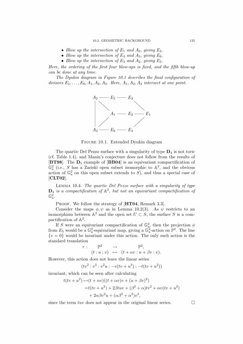
10.2. GEOMETRIC BACKGROUND 135
• Blow up the intersection of E1 and A3, giving E4.• Blow up the intersection of E4 and A3, giving E6.• Blow up the intersection of E3 and A2, giving E5.
Here, the ordering of the first four blow-ups is fixed, and the fifth blow-upcan be done at any time.
The Dynkin diagram in Figure 10.1 describes the final configuration ofdivisors E1, . . . , E6, A1, A2, A3. Here, A1, A2, A3 intersect at one point.
A2
BBBB
BBBB
E5 E3
BBBB
BBBB
A1 E2 E1
A3
||||||||E6 E4
||||||||
Figure 10.1. Extended Dynkin diagram
The quartic Del Pezzo surface with a singularity of type D4 is not toric(cf. Table 1.4), and Manin’s conjecture does not follow from the results of[BT98]. The D5 example of [BB04] is an equivariant compactification ofG2
a (i.e., S has a Zariski open subset isomorphic to A2, and the obviousaction of G2
a on this open subset extends to S), and thus a special case of[CLT02].
Lemma 10.4. The quartic Del Pezzo surface with a singularity of typeD4 is a compactification of A2, but not an equivariant compactification ofG2
a.
Proof. We follow the strategy of [HT04, Remark 3.3].Consider the maps φ, ψ as in Lemma 10.2(3). As ψ restricts to an
isomorphism between A2 and the open set U ⊂ S, the surface S is a com-pactification of A2.
If S were an equivariant compactification of G2a, then the projection φ
from E5 would be a G2a-equivariant map, giving a G2
a-action on P2. The line{v = 0} would be invariant under this action. The only such action is thestandard translation
τ : P2 → P2,(t : u : v) 7→ (t+ αv : u+ βv : v).
However, this action does not leave the linear series
(tv2 : v3 : v2u : −v(tv + u2) : −t(tv + u2))
invariant, which can be seen after calculating
t(tv + u2) 7→(t+ αv)((t+ αv)v + (u+ βv)2)
=t(tv + u2) + 2βtuv + (β2 + α)tv2 + αv(tv + u2)
+ 2αβv2u+ (αβ2 + α2)v3,
since the term tuv does not appear in the original linear series. �
136 10. MANIN’S CONJECTURE FOR A SINGULAR QUARTIC SURFACE
10.3. Manin’s conjecture
The following lemma shows that our result agrees with the prediction ofManin’s conjecture.
Lemma 10.5. Let S be the surface (10.1). Manin’s conjecture for Sstates that the number of rational points of height ≤ B outside the two linesis given by
NU,H(B) ∼ cS,H ·B(logB)5,
where cS,H = α(S) · β(S) · ωH(S) with
α(S) = (5! · 4 · 2 · 3 · 3 · 2 · 2)−1 = (34560)−1
β(S) = 1
ωH(S) = ω∞ ·∏p
(1− 1/p)6(1 + 6/p+ 1/p2)
and
ω∞ = 3∫ ∫ ∫
{(t,u,v)∈R3| 0≤v≤1, |tv2|,|v2u|,|v(tv+u2)|,|t(tv+u2)|≤1}1dtdudv.
Proof. Since S is split over Q, we have rk(Pic(S)) = 6, so the expectedexponent of logB is 5. Further, β(S) = 1. The computation of cS,H is doneon the desingularization S. The constant α(S) can be calculated as α′/#Wby Theorem 8.5, where α′ = 1/180 is the constant associated to smooth splitquartic surfaces (see Theorem 8.3), and #W = 192 is the order of the Weylgroup associated to the root system D4. The constant ωH(S) is computedas in [BB04, Lemma 1] and Lemma 9.2. �
10.4. The universal torsor
By Section 7.1, the problem of counting rational points of bounded heighton the surface S translates into a counting problem for certain integral pointson the universal torsor, subject to coprimality and height inequalities. Inthe first part of this section, we describe these conditions in detail. They areobtained by a process of introducing new variables which are the greatestcommon divisors of other variables. Geometrically, this corresponds to therealization of S as a blow-up of P2 in five points.
In the second part, we prove our claims.
The universal torsor TeS of S is an open subset of the hypersurface inA9 = Spec Z[η1, . . . , η6, α1, α2, α3] defined by the equation
(10.2) T (η,α) = α21η2 + α2η3η
25 + α3η4η
26 = 0.
The projection Ψ : TeS → S is defined by(10.3)
(Ψ∗(xi)) = (η(2,1,2,1,2,0)α2, η(4,2,3,3,2,2), η(3,2,2,2,1,1)α1, η
(2,1,1,2,0,2)α3, α2α3),
where we use the notation η(n1,n2,n3,n4,n5,n6) = ηn11 ηn2
2 ηn33 ηn4
4 ηn55 ηn6
6 .The coprimality conditions can be derived from the extended Dynkin
diagram (see Figure 10.1). Two variables are allowed to have a commonfactor if and only if the corresponding divisors (Ei for ηi and Ai for αi)

10.4. THE UNIVERSAL TORSOR 137
intersect (i.e., are connected by an edge in the diagram). Furthermore,gcd(α1, α2, α3) > 1 is allowed (corresponding to the fact that A1, A2, A3
intersect in one point).We will show below that there is a bijection between rational points
on U ⊂ S and integral points on an open subset of TeS , subject to thesecoprimality conditions.
We will later refer to
coprimalities between η1, . . . , η6 as in Figure 10.1,(10.4)
gcd(α1, η1η3η4η5η6) = 1,(10.5)
gcd(α2, η1η2η3η4η6) = 1,(10.6)
gcd(α3, η1η2η3η4η5) = 1.(10.7)
To count the number of x ∈ S(Q) such that H(x) ≤ B, we must lift thiscondition to the universal torsor, i.e., H(Ψ(η,α)) ≤ B. This is the same as
|η(2,1,2,1,2,0)α2| ≤ B, . . . , |α2α3| ≤ B,
using the five monomials occurring in (10.3). These have no common factors,provided the coprimality conditions are fulfilled (direct verification).
It will be useful to write the height conditions as follows. Let
X0 =
(η(4,2,3,3,2,2)
B
)1/3
andX1 = (Bη(−1,−2,0,0,1,1))1/3, X2 = (Bη(2,1,0,3,−2,4))1/3.
Then
|X30 | ≤ 1(10.8)
|X20 (α1/X1)| ≤ 1(10.9)
|X20 (α2/X2)| ≤ 1, |X0(X0(α2/X2) + (α1/X1)2)| ≤ 1,
|(α2/X2)(X0(α2/X2) + (α1/X1)2)| ≤ 1(10.10)
are equivalent to the five height conditions. Here we have used the torsorequation to eliminate α3 because in our counting argument we will also usethat α3 is determined by the other variables.
We now prove the above claims.
Lemma 10.6. The map Ψ gives a bijection between the set of points x ofU(Q) such that H(x) ≤ B and the set
T1 :=
{(η,α) ∈ Z6
>0 × Z3
∣∣∣∣∣equation (10.2),
coprimality (10.4), (10.5), (10.6), (10.7),
inequalities (10.8), (10.9), (10.7) hold
}
Proof. The map ψ of Lemma 10.2(3) induces a bijection
ψ0 : (η3, α1, α2) 7→ (η23α2, η
33, η
23α1, η3α3, α2α3),
where α3 := −(η3α2 + α21), i.e.,
T0 := α21 + η3α2 + α3 = 0,

138 10. MANIN’S CONJECTURE FOR A SINGULAR QUARTIC SURFACE
between
{(η3, α1, α2) ∈ Z>0 × Z2 | gcd(η3, α1, α2) = 1} and U(Q) ⊂ S(Q).
The height function on U(Q) is given by
H(ψ0(η3, α1, α2)) =max(|η2
3α2|, |η33|, |η2
3α1|, |η3α3|, |α2α3|)gcd(η2
3α2, η33, η
23α1, η3α3, α2α3)
.
The derivation of the torsor equation from the map ψ0 together with thecoprimality conditions and the lifted height function is parallel to the blow-up process described in Lemma 10.3. More precisely, each line E3, A1, A2
in P2 corresponds to a coordinate function η3, α1, α2 vanishing in one of thelines; the blow-up of the intersection of two divisors gives an exceptionaldivisor Ei, corresponding to the introduction of a new variable ηi as thegreatest common divisor of two old variables. Two divisors are disjoint ifand only if the corresponding variables are coprime. This is summarized inTable 10.1.
Variables, Equations Geometryvariables divisorsinitial variables coordinate linesη3, α1, α2 E3, A1, A2
taking gcd of two variables blowing up intersection of divisorsnew gcd-variable exceptional divisorη2, η1, η4, η6, η5 E2, E1, E4, E6, E5
extra variable extra curveα3 A3
starting relation starting descriptionα3 = −(η3α2 + α2
1) A3 = {η3α2 + α21 = 0}
final relation torsor equationα3η4η
26 = −(α2η3η
25 + α2
1η2) α21η2 + α2η3η
25 + α3η4η
26 = 0
Table 10.1. Dictionary between gcd-process and blow-ups
This plan will now be implemented in five steps; at each step, the map
ψi : Zi+1>0 × Z3 → U(Q)
gives a bijection between the following two sets:• The set of all (ηj , α1, α2, α3) ∈ Zi+1
>0 × Z3 satisfying certain co-primality conditions (described by the extended Dynkin diagramcorresponding to the i-th blow-up of Lemma 10.3), an equation Ti,and
H(ψi(ηj , αj)) =maxk(|ψi(ηj , αj)k|)
gcd(ψi(ηj , αj)k)≤ B.
• The set of all x ∈ U(Q) with H(x) ≤ B.The steps are as follows:
(1) Let η2 := gcd(η3, α1) ∈ Z>0. Then
η3 = η2η′3, α1 = η2α
′1, with gcd(η′3, α
′1) = 1.

10.4. THE UNIVERSAL TORSOR 139
Since η2 | α3, we can write α3 = η2α′3. Then α′3 = −(η′3α2 + η2α
′21 ).
After renaming the variables, we have
T1 = η2α21 + η3α2 + α3 = 0
and
ψ1 : (η2, η3, α1, α2, α3) 7→ (η2η23α2 : η2
2η33 : η2
2η23α1 : η2η3α3 : α2α3).
Here, we have eliminated the common factor η2 which occurred inall five components of the image. Below, we repeat the correspond-ing transformation at each step.
(2) Let η1 := gcd(η2, η3) ∈ Z>0. Then
η2 = η1η′2, η3 = η1η
′3, with gcd(η′2, η
′3) = 1.
As η1 | α3, we write α3 = η1α′3, and we obtain:
T2 = η2α21 + η3α2 + α3 = 0
and
ψ2 : (η1, η2, η3, α1, α2, α3) 7→(η2
1η2η23α2 : η4
1η22η
33 : η3
1η22η
23α1 : η2
1η2η3α3 : α2α3).
(3) Let η4 := gcd(η1, α3) ∈ Z>0. Then
η1 = η4η′1, α3 = η4α
′3, with gcd(η′1, α
′3) = 1.
We get after removing ′ again:
T3 = η2α21 + η3α2 + η4α3 = 0
and
ψ3 : (η1, η2, η3, η4, α1, α2, α3) 7→(η2
1η2η23η4α2 : η4
1η22η
33η
34 : η3
1η22η
23η
24α1 : η2
1η2η3η24α3 : α2α3).
(4) Let η6 := gcd(η4, α3) ∈ Z>0. Then
η4 = η6η′4, α3 = η6α
′3, with gcd(η′4, α
′3) = 1.
We obtain
T4 = η2α21 + η3α2 + η4η
26α3 = 0
and
ψ4 : (η1, η2, η3, η4, η6, α1, α2, α3) 7→(η2
1η2η23η4α2 : η4
1η22η
33η
34η
26 : η3
1η22η
23η
24η6α1 : η2
1η2η3η24η
26α3 : α2α3).
(5) The final step is η5 := gcd(η3, α2) ∈ Z>0, we could have done itearlier (just as the blow-up of the intersection of E3, A2 in Lemma(10.3)). Then
η3 = η5η′3, α2 = η5α
′2, with gcd(η′3, α
′2) = 1.
We getT5 = η2α
21 + η3η5α2 + η4η
26α3 = 0
140 10. MANIN’S CONJECTURE FOR A SINGULAR QUARTIC SURFACE
and
ψ5 : (η1, η2, η3, η4, η5, η6, α1, α2, α3) 7→(η2
1η2η23η4η
25α2 : η4
1η22η
33η
34η
25η
26 : η3
1η22η
23η
24η5η6α1 : η2
1η2η3η24η
26α3 : α2α3).
We observe that at each stage the coprimality conditions correspond to inter-section properties of the respective divisors. The final result is summarizedin Figure 10.1, which encodes data from (10.4), (10.5), (10.6), (10.7).
Note that ψ5 is Ψ from (10.3). As mentioned above, gcd(ψ5(ηj , αj)k)(over all five components of the image) is trivial by the coprimality conditionsof Figure 10.1. Therefore, H(ψ5(η,α)) ≤ B is equivalent to (10.8), (10.9),(10.10).
Finally, T5 is the torsor equation T (10.2). �
10.5. Summations
In the first step, we estimate the number of (α1, α2, α3) ∈ Z3 which fulfillthe torsor equation T (10.2) and the height and coprimality conditions. Forfixed (α1, α2), the torsor equation T has a solution α3 if and only if thecongruence
α21η2 + α2η3η
25 ≡ 0 (mod η4η
26)
holds and the conditions on the height and coprimalities are fulfilled.We have already written the height conditions so that they do not de-
pend on α3. For the coprimality, we must ensure that (10.6) and (10.7) arefulfilled.
As gcd(η3η25, η4η
26) = 1, we can find the multiplicative inverse c1 of η3η
25
modulo η4η26, so that
(10.11) c1η3η25 = 1 + c2η4η
26
for a suitable c2. Choosing
α2 = c3η4η26 − c1α
21η2,(10.12)
α3 = c2α21η2 − c3η3η
25(10.13)
gives a solution of (10.2) for any c3 ∈ Z.Without the coprimality conditions, the number of pairs (α2, α3) satis-
fying T and (10.10) would differ at most by O(1) from 1/η4η26 of the length
of the interval described by (10.10). However, the coprimality conditions(10.6) and (10.7) impose further restrictions on the choice of c3. A slightcomplication arises from the fact that because of T , some of the conditionsare fulfilled automatically once η, α1 satisfy (10.4) and (10.5).
Conditions (10.4) imply that the possibilities for a prime p to dividemore than one of the ηi are very limited. We distinguish twelve cases, listedin Column 2 of Table 10.2.
In Columns 4 and 5, we have denoted the relevant information for thedivisibility of α2, α3 by primes p which are divisors of the ηi in Column 2,but of no other ηj :
• “allowed” means that αi may be divisible by p.• “automatically” means that the conditions on the ηi and the otherαj imply that p - αi. These two cases do not impose conditions onc3 modulo p.

10.5. SUMMATIONS 141
case p | . . . p | α1 p | α2 p | α3
0 − allowed allowed allowedi η1 restriction restriction restrictionii η2 allowed restriction automaticallyiii η3 restriction restriction automaticallyiv η4 restriction automatically restrictionv η5 restriction allowed automaticallyvi η6 restriction automatically allowedvii η1, η2 restriction restriction automaticallyviii η1, η3 restriction restriction automaticallyix η1, η4 restriction automatically restrictionx η3, η5 restriction restriction automaticallyxi η4, η6 restriction automatically restriction
Table 10.2. Coprimality conditions
• “restriction” means that c3 is not allowed to be in a certain congru-ence class modulo p in order to fulfill the condition that p must notdivide αi.
The information in the table is derived as follows:
• If p | η3, then p - c2 from (10.11), and p - α1η2 because of (10.4),(10.5), so by (10.13), p - α3 independently of the choice of c3. Sincep - η4η
26, we see from (10.12) that p | α2 for one in p subsequent
choices of c3 which we must therefore exclude. This explains casesiii and viii.
• In case vii, the same is true for α2. More precisely, we see that wemust exclude c3 ≡ 0 (mod p). By (10.13), p - c3 implies that p - α3,so we do not need another condition on c3.
• In case i, we see that p | α2 for one in p subsequent choices of c3,and the same holds for α3. However, in this case, p cannot divideα2, α3 for the same choice of c3, as we can see by considering T :since p - α2
1η2, it is impossible that p | α2, α3. Consequently, wemust exclude two out of p subsequent choices of p in order to fulfillp - α2, α3.
• In the other cases, the arguments are similar.
The number of (α2, α3) ∈ Z2 subject to T , (10.6), (10.7), (10.10) equalsthe number of c3 such that α2, α3 as in (10.12), (10.13) satisfy these condi-tions. This can be estimated as 1/η4η
26 of the length of the interval described
by (10.10), multiplied by a product of local factors whose values can be readoff from Columns 2, 4, 5 of Table 10.2: the divisibility properties of ηi by pdetermine whether zero, one or two out of p subsequent values of c3 have tobe excluded. Different primes can be considered separately, and we define
ϑ1,p :=
1− 2/p, case i,1− 1/p, cases ii, . . . , iv, vi, . . . , xi,1, cases 0, v.
142 10. MANIN’S CONJECTURE FOR A SINGULAR QUARTIC SURFACE
Letϑ1(η) =
∏p
ϑ1,p
be the product of these local factors, and
(10.14) g1(u, v) =∫{t∈R| |tv2|,|t(tv+u2)|,|v(tv+u2)|≤1}
1dt.
Let ω(n) denote the number of primes dividing n.
Lemma 10.7. For fixed (η, α1) ∈ Z6>0 × Z as in (10.4), (10.5), (10.8),
(10.9), the number of (α2, α3) ∈ Z2 satisfying T , (10.6), (10.7), (10.10) is
N1(η, α1) =ϑ1(η)X2
η4η26
g1(α1/X1, X0) +O(2ω(η1η2η3η4η6)).
The sum of error terms for all possible values of (η, α1) is � B(logB)3.
Proof. The number of c3 such that the resulting α2, α3 satisfy (10.10)differs from X2
η4η26g1(α1/X1, X0) by at most O(1).
Each ϑ1,p 6= 1 corresponds to a congruence condition on c3 imposedby one of the cases i, . . . , iv, vi, . . . , xi. For each congruence condition, theactual ratio of allowed c3 can differ at most by O(1) from the ϑ1,p. The totalnumber of these primes p is
ω(η1η2η3η4η6) � 2ω(η1η2η3η4η6),
which is independent of η5 since any prime dividing only η5 contributes atrivial factor (see case v).
Using the estimate (10.9) for α1 in the first step and ignoring (10.4)(10.5), which can only increase the error term, we obtain:∑
η
∑α1
2ω(η1η2η3η4η6) ≤∑η
B · 2ω(η1η2η3η4η6)
η(3,2,2,2,1,1)� B(logB)3.
Here, we use 2ω(n)�εnε for the summations over η1, η2, η3, η4. For η6, we
employ ∑n≤x
2ω(n) � x(log x)
together with partial summation, contributing a factor (logB)2, while thesummation over η5 gives another factor logB. �
Next, we sum over all α1 subject to the coprimality condition (10.5) andthe height condition (10.9). Let
(10.15) g2(v) =∫{u∈R| |v2u|≤1}
g1(u, v)du.
Similar to our discussion for α2, α3, the number of possible values for α1 asin (10.9), while ignoring (10.5) for the moment, is X1g2(X0) +O(1).
None of the coprimality conditions are fulfilled automatically, and onlycommon factors with η2 are allowed (see Column 3 of Table 10.2). Therefore,each prime factor of η1η3η4η5η6 reduces the number of allowed α1 by a factor

10.5. SUMMATIONS 143
of ϑ2,p = 1− 1/p with an error of at most O(1). For all other primes p, letϑ2,p = 1, and let
ϑ2(η) =∏p
ϑ2,p and ϑ(η) =
{ϑ1(η) · ϑ2(η), (10.4) holds0, otherwise.
Lemma 10.8. For fixed η ∈ Z6>0 as in (10.4), (10.8), the sum of N1(η, α1)
over all α1 ∈ Z satisfying (10.5), (10.9) is
N2(η) :=ϑ(η)X1X2
η4η26
g2(X0) +R2(η),
where the sum of error terms R2(η) over all possible η is � B logB.
Proof. Let
N (b1, b2) = ϑ1(η) ·#{α1 ∈ [b1, b2] | gcd(α1, η1η3η4η5η6) = 1}.Using Mobius inversion, this is estimated as
N (b1, b2) = ϑ1(η) · ϑ2(η) · (b2 − b1) +R(b1, b2)
with R(b1, b2) = O(2ω(η1η3η4η5η6)). By partial summation,
N2(η) =ϑ(η)X1X2
η4η26
g2(X0) +R2(η)
with
R2(η) =−X2
η4η26
∫{u| |X2
0u|≤1}(D1g1)(u,X0)R(−X1/X
20 , X1u)du
where D1g1 is the partial derivative of g1 with respect to the first variable.Using the above bound for R(b1, b2), we obtain:
R2(η) � X2
η4η26
2ω(η1η3η4η5η6).
Summing this over all η as in (10.8) while ignoring (10.4) which can onlyenlarge the sum, we obtain∑
η
R2(η) �∑η
X2 · 2ω(η1η3η4η5η6)
η4η26X
20
=∑η
B · 2ω(η1η3η4η5η6)
η(2,1,2,2,2,2)� B logB.
In the first step, we use X0 ≤ 1. �
Let
∆(n) = B−2/3∑
ηi,η(4,2,3,3,2,2)=n
ϑ(η)X1X2
η4η26
=∑
ηi,η(4,2,3,3,2,2)=n
ϑ(η)(η(4,2,3,3,2,2))1/3
η(1,1,1,1,1,1).
In view of Lemma 10.6, the number of rational points of bounded heighton U can be estimated by summing the result of Lemma 10.8 over all suitableη. The error term is the combination of the error terms in Lemmas 10.7 and10.8.
Lemma 10.9. We have
NU,H(B) = B2/3∑n≤B
∆(n)g2((n/B)1/3) +O(B(logB)3).

144 10. MANIN’S CONJECTURE FOR A SINGULAR QUARTIC SURFACE
10.6. Completion of the proof
We need an estimate for
M(t) :=∑n≤t
∆(n).
Consider the Dirichlet series F (s) :=∑∞
n=1 ∆(n)n−s. Using
F (s+ 1/3) =∑η
ϑ(η)η4s+11 η2s+1
2 η3s+13 η3s+1
4 η2s+15 η2s+1
6
,
we write F (s + 1/3) =∏
p Fp(s + 1/3) as its Euler product. To obtainFp(s+1/3) for a prime p, we need to restrict this sum to the terms in whichall ηi are powers of p. Note that ϑ(η) is non-zero if and only if the divisibilityof ηi by p falls into one of the twelve cases described in Table 10.2. The valueof ϑ(η) only depends on these cases.
Writing Fp(s+ 1/3) =∑11
i=0 Fp,i(s+ 1/3), we have for example:
Fp,0(s+ 1/3) = 1,
Fp,1(s+ 1/3) =∞∑
j=1
(1− 1/p)(1− 2/p)pj(4s+1)
=(1− 1/p)(1− 2/p)
p4s+1 − 1,
Fp,7(s+ 1/3) =∞∑
j,k=1
(1− 1/p)2
pj(4s+1)pk(2s+1)=
(1− 1/p)2
(p4s+1 − 1)(p2s+1 − 1).
The other cases are similar, giving
Fp(s+ 1/3) =1 +1− 1/pp4s+1 − 1
((1− 2/p) +
1− 1/pp2s+1 − 1
+ 21− 1/pp3s+1 − 1
)+
1− 1/pp2s+1 − 1
+ 2(1− 1/p)2
p3s+1 − 1+ 2
1− 1/pp2s+1 − 1
+ 2(1− 1/p)2
(p2s+1 − 1)2.
Defining
E(s) := ζ(4s+ 1)ζ(3s+ 1)2ζ(2s+ 1)3 and G(s) := F (s+ 1/3)/E(s),
we see as in Section 9.6 that the residue of F (s)ts/s at s = 1/3 is
Res(t) =3G(0)t1/3Q1(log t)5! · 4 · 2 · 3 · 3 · 2 · 2
for a monic Q1 ∈ R[x] of degree 5. By Lemma 10.5, α(S) = 15!·4·2·3·3·2·2 . By
a Tauberian argument as in Lemma 9.13:
Lemma 10.10. M(t) = Res(t) +O(t1/3−δ) for some δ > 0.
By partial summation,∑n≤B
∆(n)g2((n/B)1/3) = α(S)G(0)B1/3Q(logB) · 3∫ 1
0g2(v)dv +O(B
13−δ)
for a monic polynomial Q of degree 5. We identify ωH(S) from
G(0) =∏p
(1− 1
p
)6(1 +
6p
+1p2
), and ω∞ = 3
∫ 1
0g2(v)dv.
Together with Lemma 10.9, this completes the proof of Theorem 10.1.
Bibliography
[AN04] V. Alexeev and V. V. Nikulin. Classification of log del Pezzo surfaces of index≤ 2, arXiv:math.AG/0406536, 2004.
[Art66] M. Artin. On isolated rational singularities of surfaces. Amer. J. Math., 88:129–136, 1966.
[BB04] R. de la Breteche and T. D. Browning. On Manin’s conjecture for sin-gular del Pezzo surfaces of degree four, I. Mich. Math. J., to appear,arXiv:math.NT/0412086, 2004.
[BB05] R. de la Breteche and T. D. Browning. On Manin’s conjecture for singulardel Pezzo surfaces of degree four, II. Math. Proc. Camb. Phil. Soc., to appear,arXiv:math.NT/0502510, 2005.
[BBD05] R. de la Breteche, T. D. Browning, and U. Derenthal. On Manin’s conjec-
ture for a certain singular cubic surface. Ann. Sci. Ecole Norm. Sup. (4),arXiv:math.NT/0509370, 2005.
[BF04] R. de la Breteche and E. Fouvry. L’eclate du plan projectif en quatre pointsdont deux conjugues. J. Reine Angew. Math., 576:63–122, 2004.
[Bir62] B. J. Birch. Forms in many variables. Proc. Roy. Soc. Ser. A, 265:245–263,1961/1962.
[BM90] V. V. Batyrev and Yu. I. Manin. Sur le nombre des points rationnels de hauteurborne des varietes algebriques. Math. Ann., 286(1-3):27–43, 1990.
[BP04] V. V. Batyrev and O. N. Popov. The Cox ring of a del Pezzo surface. In Arith-metic of higher-dimensional algebraic varieties (Palo Alto, CA, 2002), volume226 of Progr. Math., pages 85–103. Birkhauser Boston, Boston, MA, 2004.
[Bre98] R. de la Breteche. Sur le nombre de points de hauteur bornee d’une certainesurface cubique singuliere. Asterisque, (251):51–77, 1998. Nombre et repartitionde points de hauteur bornee (Paris, 1996).
[Bre02] R. de la Breteche. Nombre de points de hauteur bornee sur les surfaces de delPezzo de degre 5. Duke Math. J., 113(3):421–464, 2002.
[Bro89] K. S. Brown. Buildings. Springer-Verlag, New York, 1989.[Bro04] T. D. Browning. The density of rational points on a certain singular cubic
surface, arXiv:math.NT/0404245, 2004.[Bro05] T. D. Browning. An overview of Manin’s conjecture for del Pezzo surfaces,
arXiv:math.NT/0511041, 2005.[BT95] V. V. Batyrev and Yu. Tschinkel. Rational points of bounded height on com-
pactifications of anisotropic tori. Internat. Math. Res. Notices, (12):591–635,1995.
[BT98] V. V. Batyrev and Yu. Tschinkel. Manin’s conjecture for toric varieties. J. Al-gebraic Geom., 7(1):15–53, 1998.
[BW79] J. W. Bruce and C. T. C. Wall. On the classification of cubic surfaces. J. LondonMath. Soc. (2), 19(2):245–256, 1979.
[Cay69] A. Cayley. A memoir on cubic surfaces. Philos. Trans. Roy. Soc. London,159:231–326, 1869.
[CLT02] A. Chambert-Loir and Yu. Tschinkel. On the distribution of points of boundedheight on equivariant compactifications of vector groups. Invent. Math.,148(2):421–452, 2002.
[Cox95] D. A. Cox. The homogeneous coordinate ring of a toric variety. J. AlgebraicGeom., 4(1):17–50, 1995.
145

146 BIBLIOGRAPHY
[CT88] D. F. Coray and M. A. Tsfasman. Arithmetic on singular Del Pezzo surfaces.Proc. London Math. Soc. (3), 57(1):25–87, 1988.
[CTS80] J.-L. Colliot-Thelene and J.-J. Sansuc. La descente sur les varietes rationnelles.In Journees de Geometrie Algebrique d’Angers, Juillet 1979/Algebraic Geome-try, Angers, 1979, pages 223–237. Sijthoff & Noordhoff, Alphen aan den Rijn,1980.
[CTS87] J.-L. Colliot-Thelene and J.-J. Sansuc. La descente sur les varietes rationnelles.II. Duke Math. J., 54(2):375–492, 1987.
[Der05] U. Derenthal. Manin’s conjecture for a certain singular cubic surface,arXiv:math.NT/0504016, 2005.
[Der06a] U. Derenthal. On a constant arising in Manin’s conjecture for Del Pezzo surfaces,2006.
[Der06b] U. Derenthal. On the Cox ring of Del Pezzo surfaces, arXiv:math.AG/0603111,2006.
[Der06c] U. Derenthal. Singular Del Pezzo surfaces whose universal torsors are hypersur-faces, arXiv:math.AG/0604194, 2006.
[Der06d] U. Derenthal. Universal torsors of Del Pezzo surfaces and homogeneous spaces,arXiv:math.AG/0604195, 2006.
[Dol03] I. Dolgachev. Lectures on invariant theory, volume 296 of London MathematicalSociety Lecture Note Series. Cambridge University Press, Cambridge, 2003.
[DP80] M. Demazure and H. C. Pinkham, editors. Seminaire sur les Singularites desSurfaces, volume 777 of Lecture Notes in Mathematics. Springer, Berlin, 1980.
Held at the Centre de Mathematiques de l’Ecole Polytechnique, Palaiseau, 1976–1977.
[DT06] U. Derenthal and Yu. Tschinkel. Universal torsors over Del Pezzo surfaces andrational points. In Equidistribution in Number Theory, An Introduction (Mon-treal, 2005), to appear, NATO Sci. Ser. II Math. Phys. Chem., Dordrecht, 2006.Springer.
[DV34] P. Du Val. On isolated singularities of surfaces which do not affect the conditionsof adjunction (parts ii and iii). Proc. Cambridge Philos. Soc., 30:460–465, 483–491, 1934.
[EKW04] E. J. Elizondo, K. Kurano, and K. Watanabe. The total coordinate ring of anormal projective variety. J. Algebra, 276(2):625–637, 2004.
[FM02] R. Friedman and J. W. Morgan. Exceptional groups and del Pezzo surfaces. InSymposium in Honor of C. H. Clemens (Salt Lake City, UT, 2000), volume 312of Contemp. Math., pages 101–116. Amer. Math. Soc., Providence, RI, 2002.
[FMT89] J. Franke, Yu. I. Manin, and Yu. Tschinkel. Rational points of bounded heighton Fano varieties. Invent. Math., 95(2):421–435, 1989.
[Fou98] E. Fouvry. Sur la hauteur des points d’une certaine surface cubique singuliere.Asterisque, (251):31–49, 1998. Nombre et repartition de points de hauteurbornee (Paris, 1996).
[Fre53] H. Freudenthal. Sur le groupe exceptionnel E7. Nederl. Akad. Wetensch. Proc.Ser. A. 56=Indagationes Math., 15:81–89, 1953.
[Ful93] W. Fulton. Introduction to toric varieties, volume 131 of Annals of Mathemat-ics Studies. Princeton University Press, Princeton, NJ, 1993. The William H.Roever Lectures in Geometry.
[GJ00] E. Gawrilow and M. Joswig. polymake: a framework for analyzing convex poly-topes. In Polytopes—combinatorics and computation (Oberwolfach, 1997), vol-ume 29 of DMV Sem., pages 43–73. Birkhauser, Basel, 2000.
[Har77] R. Hartshorne. Algebraic geometry. Springer-Verlag, New York, 1977. GraduateTexts in Mathematics, No. 52.
[Has04] B. Hassett. Equations of universal torsors and Cox rings. In MathematischesInstitut, Georg-August-Universitat Gottingen: Seminars Summer Term 2004,pages 135–143. Universitatsdrucke Gottingen, Gottingen, 2004.
[HB03] D. R. Heath-Brown. The density of rational points on Cayley’s cubic surface. InProceedings of the Session in Analytic Number Theory and Diophantine Equa-tions, volume 360 of Bonner Math. Schriften, page 33, Bonn, 2003. Univ. Bonn.

BIBLIOGRAPHY 147
[HBM99] D. R. Heath-Brown and B. Z. Moroz. The density of rational points on the cubicsurface X3
0 = X1X2X3. Math. Proc. Cambridge Philos. Soc., 125(3):385–395,1999.
[HK00] Y. Hu and S. Keel. Mori dream spaces and GIT. Michigan Math. J., 48:331–348,2000. Dedicated to William Fulton on the occasion of his 60th birthday.
[HT04] B. Hassett and Yu. Tschinkel. Universal torsors and Cox rings. In Arithmeticof higher-dimensional algebraic varieties (Palo Alto, CA, 2002), volume 226 ofProgr. Math., pages 149–173. Birkhauser Boston, Boston, MA, 2004.
[Kle66] S. L. Kleiman. Toward a numerical theory of ampleness. Ann. of Math. (2),84:293–344, 1966.
[Lur01] J. Lurie. On simply laced Lie algebras and their minuscule representations.Comment. Math. Helv., 76(3):515–575, 2001.
[Man86] Yu. I. Manin. Cubic forms, volume 4 of North-Holland Mathematical Library.North-Holland Publishing Co., Amsterdam, second edition, 1986. Algebra, ge-ometry, arithmetic, Translated from the Russian by M. Hazewinkel.
[MS72] D. Mumford and K. Suominen. Introduction to the theory of moduli. In Alge-braic geometry, Oslo 1970 (Proc. Fifth Nordic Summer-School in Math.), pages171–222. Wolters-Noordhoff, Groningen, 1972.
[Pey95] E. Peyre. Hauteurs et mesures de Tamagawa sur les varietes de Fano. DukeMath. J., 79(1):101–218, 1995.
[Pey98] E. Peyre. Terme principal de la fonction zeta des hauteurs et torseurs universels.Asterisque, (251):259–298, 1998. Nombre et repartition de points de hauteurbornee (Paris, 1996).
[Pey04] E. Peyre. Counting points on varieties using universal torsors. In Arithmeticof higher-dimensional algebraic varieties (Palo Alto, CA, 2002), volume 226 ofProgr. Math., pages 61–81. Birkhauser Boston, Boston, MA, 2004.
[Pop01] O. N. Popov. Del Pezzo surfaces and algebraic groups, Diplomarbeit, UniversitatTubingen, 2001.
[PT01a] E. Peyre and Yu. Tschinkel. Tamagawa numbers of diagonal cubic surfaces,numerical evidence. Math. Comp., 70(233):367–387, 2001.
[PT01b] E. Peyre and Yu. Tschinkel. Tamagawa numbers of diagonal cubic surfaces ofhigher rank. In Rational points on algebraic varieties, volume 199 of Progr.Math., pages 275–305. Birkhauser, Basel, 2001.
[Sal98] P. Salberger. Tamagawa measures on universal torsors and points of boundedheight on Fano varieties. Asterisque, (251):91–258, 1998. Nombre et repartitionde points de hauteur bornee (Paris, 1996).
[Sch63] L. Schlafli. On the distribution of surfaces of the thrid order into species, inreference to the absence or presence of singular points, and the relaity of theirlines. Philos. Trans. Roy. Soc. London, 153:193–241, 1863.
[Seg42] B. Segre. The non-singular cubic surfaces. Clarendon, Oxford, 1942.[Sko93] A. N. Skorobogatov. On a theorem of Enriques-Swinnerton-Dyer. Ann. Fac.
Sci. Toulouse Math. (6), 2(3):429–440, 1993.[Tim28] G. Timms. The nodal cubic surfaces and the surfaces from which they are
derived by projection. Proc. Roy. Soc. London Ser. A, 119:213–248, 1928.[Zie95] G. M. Ziegler. Lectures on polytopes, volume 152 of Graduate Texts in Mathe-
matics. Springer-Verlag, New York, 1995.


Index
algebraic group, 45anticanonical class, 7, 9, 10, 59, 83, 109automorphism of P2, 12, 22
base point, 82blow-up, 8, 10, 15, 20, 59
canonical class, 7Castelnuovo, 21chamber, 13, 110
fundamental, 13, 18, 110, 113character, 26circle method, 102, 104cohomology group, 25, 105complete intersection, 47, 106cone
affine, 45convex, 10effective, 10, 12, 16, 27, 59, 105, 109,
114nef, 10, 59, 109
contraction, 20, 83coprimality condition, 2, 119, 136Cox ring, 2, 27, 31, 46, 57, 81
generator, 27, 31, 35, 38, 58, 82, 89,93
relation, 29, 31, 33, 35, 43, 58, 86, 89cubic surface, 73
Cayley’s, 88E6, 16, 28, 107, 117singular, 3, 7, 16, 19, 21, 93smooth, 1, 11, 19, 34, 53
curve(−1)-, 11, 18, 31, 34, 38, 40(−2)-, 16negative, 28, 58, 102
degree, 8Del Pezzo surface
degree 1, 40degree 2, 38, 55degree 3, see also cubic surfacedegree 4, see also quartic surfacedegree 5, 63degree 6, 61
generalized, 15, 17, 57, 81, 102, 113singular, 15, 102, 113smooth, 2, 8, 11, 15, 31, 45, 101, 111toric, 29
density, 106Dirichlet series, 129, 144distinguished section, 83divisor, 7
effective, 7, 27exceptional, 9, 15, 134prime, 7
divisor group, 7Dynkin diagram, 13, 15
extended, 16–18, 34, 59, 89, 94, 136
embedding, 45anticanonical, 11, 16, 34, 59
error term, 107, 118
familyembedding, 46, 56generalized, 22, 96smooth, 12
Fano variety, 101flag variety, 45
global section, 27grading, 27Grassmannian, 3
halfspace, 13height, 1, 101, 117, 133height inequality, 2, 104, 124, 137height zeta function, 103, 106Hirzebruch surface, 16, 21, 22, 111homogeneous coordinate ring, 27homogeneous space, 3, 47hypersurface, 101, 103
universal torsor, 57, 118, 133
integral point, 2, 103, 119, 136intersection form, 7, 18intersection matrix, 18, 59intersection number, 7irreducible, 29, 87Iskovskih surface, 105
149
150 INDEX
Lebesgue measure, 109Leray form, 106, 119Leray measure, 106line, 1, 11, 34, 102linear system, 82
Manin’s conjecture, 2, 102, 118, 133meromorphic continuation, 107minimal desingularization, 15
non-split, 102, 133
parabolic, 45partial ordering, 9, 27passing through, 10Peyre’s constant, 102, 105, 109, 118, 133Picard group, 2, 7, 9, 104
basis, 59standard basis, 10
pole, 107position
almost general, 15, 16, 102general, 11
quartic surface, 66D4, 133generalized, 16, 19singular, 89smooth, 11
radical, 31, 86rational double point, 15reflection, 13, 14representation, 46
fundamental, 45rescaling, 46
good, 46, 50rescaling factor, 46residue, 107, 130, 144root, 13
positive, 13simple, 13, 18, 45, 110
root system, 13, 18, 31, 45, 110irreducible, 14, 110
ruling, 31, 32, 39, 41, 47(2)-, 39, 42(3)-, 43(n)-, 31, 111
self intersection number, 7singularity, 15, 16, 59, 110
resolution, 15, 134split, 2, 102, 109, 133summation, 125, 140surface, 7, 25
Tauberian theorem, 103, 107, 130, 144toric variety, 22torsor, 25
torus, 25Neron-Severi, 26, 29, 46
transform, 9triangle, 34type, 17
singularity, 15, 20
universal torsor, 2, 25, 26, 29, 45, 46,57, 103, 119, 136
weight, 45weight lattice, 45Weyl group, 13, 14, 18, 31, 45, 109
Lebenslauf
21. 07. 1978 Geboren in Brakel
07/1985–06/1989 Katholische Grundschule Brakel
07/1989–06/1998 Gymnasium Brede in Brakel,abgeschlossen mit dem Abitur
07/1998–04/1999 Grundwehrdienst in Dulmen
04/1999 Beginn des Studiums der Mathematik an derGeorg-August-Universitat Gottingen
04/2000 Vordiplom in Mathematik
08/2001–06/2002 Auslandsstudium an derUniversity of California, Berkeley
01/2004 Diplom in MathematikBetreuer der Diplomarbeit: Prof. Dr. U. Stuhler
seit 03/2004 Promotionsstudiumam Mathematischen Institutder Georg-August-Universitat GottingenBetreuer: Prof. Dr. Yu. Tschinkel
03/2006–05/2006 Forschungsaufenthalt am MSRI, Berkeley


![UNIVERSAL COVERING SPACES AND FUNDAMENTAL GROUPS IN … · 2019-09-29 · arXiv:0902.3464v2 [math.AG] 1 Jul 2009 UNIVERSAL COVERING SPACES AND FUNDAMENTAL GROUPS IN ALGEBRAIC GEOMETRY](https://static.documents.pub/doc/80x56/5f02870b7e708231d404b520/universal-covering-spaces-and-fundamental-groups-in-2019-09-29-arxiv09023464v2.jpg)


![Fundamental bigroupoids and 2-covering spaces...bundles [Bar06, BS07], 2-torsors [Bak07] and categorical torsors [CG01]) has been directed by category theoretic considerations or by](https://static.documents.pub/doc/80x56/6120a77849a9ac16e110ba2d/fundamental-bigroupoids-and-2-covering-spaces-bundles-bar06-bs07-2-torsors.jpg)
