Annales Geophysicae (2003) 21: 615–626 c European Geosciences Union 2003 Annales Geophysicae Photon path length distributions for cloudy skies – oxygen A-Band measurements and model calculations O. Funk and K. Pfeilsticker Institut f¨ ur Umweltphysik, University of Heidelberg, Germany Received: 1 November 2001 – Revised: 1 July 2002 – Accepted: 17 July 2002 Abstract. This paper addresses the statistics underlying cloudy sky radiative transfer (RT) by inspection of the dis- tribution of the path lengths of solar photons. Recent studies indicate that this approach is promising, since it might reveal characteristics about the diffusion process underlying atmo- spheric radiative transfer (Pfeilsticker, 1999). Moreover, it uses an observable that is directly related to the atmospheric absorption and, therefore, of climatic relevance. However, these studies are based largely on the accuracy of the mea- surement of the photon path length distribution (PPD). This paper presents a refined analysis method based on high reso- lution spectroscopy of the oxygen A-band. The method is validated by Monte Carlo simulation atmospheric spectra. Additionally, a new method to measure the effective opti- cal thickness of cloud layers, based on fitting the measured differential transmissions with a 1-dimensional (discrete or- dinate) RT model, is presented. These methods are applied to measurements conducted during the cloud radar inter- comparison campaign CLARE’98, which supplied detailed cloud structure information, required for the further analy- sis. For some exemplary cases, measured path length dis- tributions and optical thicknesses are presented and backed by detailed RT model calculations. For all cases, reasonable PPDs can be retrieved and the effects of the vertical cloud structure are found. The inferred cloud optical thicknesses are in agreement with liquid water path measurements. Key words. Meteorology and atmospheric dynamics (radia- tive processes; instruments and techniques) 1 Introduction The deposition of the solar shortwave (SW) radiation is the driving force of many atmospheric processes, such as atmo- spheric dynamics or photochemistry. Thus, it is a primary factor controlling the climate of the globe (Stephens and Correspondence to: O. Funk ([email protected]) Tsay, 1990; Wild et al., 1995, 1996, and others). Despite its important role for the terrestrial climate, the amount of SW radiation absorbed in the clear and cloudy atmosphere is still poorly understood. Under cloudy skies, the poor under- standing is primarily due to either (a) deficits in understand- ing atmospheric absorber characteristics (interstitial aerosol absorption, water vapor line strength and continuum absorp- tion or yet unknown absorption mechanism, such as water dimers) and (b) deficits in understanding the cloudy sky ra- diative transfer (e.g. results presented at the recent Chapman Conference on Atmospheric Absorption and Solar Radiation, AGU 2001). The present paper explores in more detail possibility (b) by presenting joint cloudy sky photon path length distribu- tion and cloud optical thickness measurements, cloud struc- ture data, and model calculations. The cloudy sky pho- ton path length distribution measurements were performed by means of high resolution oxygen A-band measurements in zenith scattered skylight. This type of measurement has been developing rapidly in recent years (e.g. Harrison and Min, 1997; Pfeilsticker et al., 1998). Historically, cloudy sky photon path length distributions have been shown to be ap- proximately gamma distributed in a homogenously (and in the vertical inhomogeneously) scattering atmosphere (Van de Hulst, 1980; Marshak et al., 1995). From the very beginning it was clear that scattering problems in real cloud covered atmospheres may lead to far more complicated PPDs since cloud covers tend to appear in patches, multilayers or even as fractal cloud decks (e.g. Davis et al., 1996). Thus, real scattering atmospheres require assumptions on the distribu- tion of the individual step sizes, which are different from the classical assumption of a well-defined exponential dis- tribution, the latter leading to the classical diffusion assump- tion for homogenous, optically thick media. Clearly, real at- mospheres do not fulfill this assumption, while theoretically they are more likely to support scattering statistics with indi- vidual step size distributions which allow for more frequent extreme step sizes. This lack of theoretical correctness in classical cloudy sky RT modelling led Davis and Marshak
Photon path length distributions for cloudy skies – oxygen A-Bandmeasurements and model calculations
O. Funk and K. Pfeilsticker
Institut fur Umweltphysik, University of Heidelberg, Germany
Received: 1 November 2001 – Revised: 1 July 2002 – Accepted: 17 July 2002
Abstract. This paper addresses the statistics underlyingcloudy sky radiative transfer (RT) by inspection of the dis-tribution of the path lengths of solar photons. Recent studiesindicate that this approach is promising, since it might revealcharacteristics about the diffusion process underlying atmo-spheric radiative transfer (Pfeilsticker, 1999). Moreover, ituses an observable that is directly related to the atmosphericabsorption and, therefore, of climatic relevance. However,these studies are based largely on the accuracy of the mea-surement of the photon path length distribution (PPD). Thispaper presents a refined analysis method based on high reso-lution spectroscopy of the oxygen A-band. The method isvalidated by Monte Carlo simulation atmospheric spectra.Additionally, a new method to measure the effective opti-cal thickness of cloud layers, based on fitting the measureddifferential transmissions with a 1-dimensional (discrete or-dinate) RT model, is presented. These methods are appliedto measurements conducted during the cloud radar inter-comparison campaign CLARE’98, which supplied detailedcloud structure information, required for the further analy-sis. For some exemplary cases, measured path length dis-tributions and optical thicknesses are presented and backedby detailed RT model calculations. For all cases, reasonablePPDs can be retrieved and the effects of the vertical cloudstructure are found. The inferred cloud optical thicknessesare in agreement with liquid water path measurements.
Key words. Meteorology and atmospheric dynamics (radia-tive processes; instruments and techniques)
1 Introduction
The deposition of the solar shortwave (SW) radiation is thedriving force of many atmospheric processes, such as atmo-spheric dynamics or photochemistry. Thus, it is a primaryfactor controlling the climate of the globe (Stephens and
Tsay, 1990; Wild et al., 1995, 1996, and others). Despiteits important role for the terrestrial climate, the amount ofSW radiation absorbed in the clear and cloudy atmosphere isstill poorly understood. Under cloudy skies, the poor under-standing is primarily due to either (a) deficits in understand-ing atmospheric absorber characteristics (interstitial aerosolabsorption, water vapor line strength and continuum absorp-tion or yet unknown absorption mechanism, such as waterdimers) and (b) deficits in understanding the cloudy sky ra-diative transfer (e.g. results presented at the recent ChapmanConference on Atmospheric Absorption and Solar Radiation,AGU 2001).
The present paper explores in more detail possibility (b)by presenting joint cloudy sky photon path length distribu-tion and cloud optical thickness measurements, cloud struc-ture data, and model calculations. The cloudy sky pho-ton path length distribution measurements were performedby means of high resolution oxygen A-band measurementsin zenith scattered skylight. This type of measurement hasbeen developing rapidly in recent years (e.g. Harrison andMin, 1997; Pfeilsticker et al., 1998). Historically, cloudy skyphoton path length distributions have been shown to be ap-proximately gamma distributed in a homogenously (and inthe vertical inhomogeneously) scattering atmosphere (Van deHulst, 1980; Marshak et al., 1995). From the very beginningit was clear that scattering problems in real cloud coveredatmospheres may lead to far more complicated PPDs sincecloud covers tend to appear in patches, multilayers or evenas fractal cloud decks (e.g. Davis et al., 1996). Thus, realscattering atmospheres require assumptions on the distribu-tion of the individual step sizes, which are different fromthe classical assumption of a well-defined exponential dis-tribution, the latter leading to the classical diffusion assump-tion for homogenous, optically thick media. Clearly, real at-mospheres do not fulfill this assumption, while theoreticallythey are more likely to support scattering statistics with indi-vidual step size distributions which allow for more frequentextreme step sizes. This lack of theoretical correctness inclassical cloudy sky RT modelling led Davis and Marshak
616 O. Funk and K. Pfeilsticker: Photon path length distributions for cloudy skies
(1998) to suggest Levy type diffusion, characterized by indi-vidual step size distributions decreasing according to powerlaws (in contrast to the exponential distribution in Gaussiandiffusion), to be more appropriate in cloudy sky scatteringphenomena, a suggestion experimentally supported for manycomplicated cloudy sky cases by Pfeilsticker (1999) or re-cently by Min et al. (2001). Previous oxygen A-band PPDmeasurements, however, were suffering from several limita-tions, such as a limited temporal and, hence, spatial resolu-tion at the expense of a high spectral resolution, an insuf-ficient spectral retrieval technique, and a lack of validation.While overcoming the first limitation requires more sensitiveinstrumentation, being presently developed, the other limita-tions are addressed by the methodic improvement presentedin this paper.
2 Photon path length distributions, Beer’s law and theLaplace transformation
The basic idea of cloudy sky geometrical path length distri-butions is that the sequence of scattering events form a lightpath from which finally, only the total geometrical length isrelevant. Extinction can then be regarded solely as gaseousabsorption along this path. Since multiple scattering is astochastic process, each photon will travel a different path.The probability that a photon has travelled a total path lengthl is given by the probability density function (PDF) of thegeometrical path lengthsp(l) (short PPD).
p(l)dl = P(l −1
2dl < L < l +
1
2dl) (1)
This distribution is only valid in absence of absorption,i.e. for the scattering processes only. In an absorbing atmo-sphere, the transmission with respect to absorption, describedby the absorption cross sectionσ and the number concentra-tion n, along a specific path of lengthL is given by Beer’slaw.
T (L) = exp
{−
∫ L
0σn dl
} σnconst.= exp{−αL} (2)
For constant extinctionα = σn the total transmission of alloccurring paths is given by the integral over the path lengthdistribution weighted with the Beer factor exp{−αl}.
T (α) =
∫∞
0p(l)exp{−αl} dl = Lα←lp(l) = p(α) (3)
This expression is formally equivalent to theLaplace trans-formationL of p(l) with respect toα. Thus, it is a con-sequence of the exponential form of Beer’s law thatT (α)
is the Laplace transform of the PPD. This relationship im-plies that the explicitly unmeasurable path length distributioncan be derived by measuring the transmissions for differentabsorption strengths and inverting the Laplace transforma-tion. Techniques for this non-trivial inversion are discussedin Sect. 3.
The above relation is only valid for constant extinction, i.e.in an isotropic atmosphere. In the real atmosphere mainly thepressure and temperature dependencies ofn andσ introducea vertical anisotropy. For a general atmosphere the path in-tegral in the exponent of Eq. (2) can be different for eachphoton trajectory. For an ensemble ofN photons the totaltransmissionT is then given by the ensemble average:
T =1
N
N∑i=1
exp
{−
∫ Li
0σi(l)ni(l) dl
}. (4)
The right-hand side of this equation is highly complex,since it requires the knowledge of each photon trajectory.Moreover,T cannot be expressed as an explicit function ofα.The Laplace transformation ofp(l) is, therefore, in generalnot given by the transmissionsT as in Eq. (3). Equation (4)can, however, be simplified approximately usingp(l) and amean absorption coefficientα.
T (αi, Li) ≈ T (α) =
∫∞
0p(l)exp{−α · l} dl (5)
This approximation introduces a systematic error, but itsapproximated validity can be tested by a Monte Carlo simu-lation of the photon paths in a non-isotropic atmosphere (seeSect. 4).
3 Inversion of the Laplace transformation
The possibility ofretrieving the path length distribution frommeasured transmissions is based on an accurate technique forthe calculation of the inverse Laplace transformation. Thisinversion is not straightforward. Direct techniques are un-suited (see Appendix A). Therefore, a constrained methodimposing a priori assumptions on the analytical form of thepath length distribution can be used. Most common in thiscontext is theGammadistribution. Van de Hulst (1980,17.2.3) shows that the photon optical path distribution for ho-mogeneous slabs can be well approximated by Gamma dis-tributions. Marshak et al. (1995) show that the distribution ofthe photon displacement at the point of escape from homo-geneous, as well as horizontally fractal cloud layers, is wellapproximated by Gamma distributions. The Gamma distri-bution (Eq. (6)) has two parameters,〈l〉 andκ, each beingfunctions of the first two moments of the PDF.
p(l) =1
0(κ)(〈l〉κ
)κ (l)κ−1 e−κl〈l〉 , with κ =
〈l〉2
var(l)(6)
The inversion problem is solved if the Laplace transfor-mation of the analytical expression of the PDF can be calcu-lated. For the Gamma distribution it is given by:
p(k) =1(
1+ 〈x〉κk)κ . (7)
A more general, numerical method is based on accurateforward modelling of the measured transmissions according
O. Funk and K. Pfeilsticker: Photon path length distributions for cloudy skies 617
Table 1. Scattering characteristics used for the radiative transfer models
Scattering events Cross section/extinction Phase function
Rayleigh σRS=4.02×10⁻²⁸/λ4.04cm2 (Nicolet, 1984) ψ(cosϑ)=34(1 + cos2ϑ), no polarization
to Eq. (3). In this case any parameterized expression usingparameterspi can be used as PDF,p(l) = f (l, a1, . . . , an).The parameters are then retrieved by applying a least-squaresfit of observed (measured or from radiative transfer models)and forward modelled transmissions. Another well suitedstandard distribution is the log-normal distribution:
p(l) =1
Sl√
2πexp
{−(ln l −M)2
2S2
}, (8)
with parametersM andS.The validity of these PDF models is tested with a Monte
Carlo model (see Sect. 4). For further analysis this numericalmethod with Gamma and log-normal distributions as modelsfor p(l) are used. Additionally, two modifications ofp(l) aremade for practical purposes:
– Variable transformationThe path length is measured in units of vertical pathsthrough the atmosphere. This is done by changing theindependent variable fromα to thevertical optical den-sityVOD = α ·lver . This changes the independent vari-able ofp(l) from l to l′ = l/ lver . Sinceα is not constantin the atmosphere,VOD =
∫∞
0 α(z) dz is used instead.
– Shift of the distributionSince lengths of path shorter than one vertical paththrough the atmosphere cannot occur for transmission,the distribution is shifted by one vertical path byl′ =l−lver in old, orl′ = l−1 in new variables. Applicationof the translation property of the Laplace transformationyields a factor ofe−VOD in the Laplace transform (seeEq. (A3)).
4 Validation with a Monte Carlo radiative transfermodel
The method is validated by modelling the path length dis-tributions and transmissions for the atmosphere by a MonteCarlo radiative transfer model. Since the inaccuracy of theapproximation in Eq. (5) strongly depends on the cloud sit-uation, i.e. mainly the vertical extent and vertical variabilityof the paths, two different typical cases are presented here:
Table 2. Results (momentsm1/2) of the PPD retrievals for the firsttwo moments using both PDF models for both cases. Also includedare the results of the direct fit to the MC PDF, see Fig. 1
Case PDF model Transmissions PDF direct MC modelm1 m2 m1 m2 m1 m2
1 Gamma 11.7 177 12.3 185 13.4 251
1 log-normal 12.0 196 13.5 258 13.4 251
2 Gamma 4.6 33 3.7 19 4.8 42
2 log-normal 4.7 39 4.5 37 4.8 42
– Case 1: extended cumulus cloudcloud base 1000 m,1H = 3000 m,τc = 200,λMie = 15 m,g = 0.85
– Case 2: low level stratus cloud with thin cirruscloud base 1000 m,1H = 1000 m,τc = 50,λMie = 20 m,g = 0.85
with 1H being the vertical cloud layer extent andλMie themean free path forMie scattering within the layer.
The Monte Carlo model generates the photon trajectoriesby simulating the elementary scattering processes listed inTable 1. A backward approach is used to save computationtime. The photon is injected into the atmosphere at the de-tector position in zenith viewing direction. It is then tracedalong its path. Upon escape from the model atmosphere, theprobability for the last scattering to result in the direction to-wards the Sun is calculated, and a statistical weight equalto this probability is assigned to the trajectory. In order tosimulate the transmission, the optical densities at 15 wave-lengths, located in the centers of oxygen A-band lines, areaccurately integrated along the trajectories. For that to oc-cur, the absorption cross section and number concentrationare calculated according to a temperature profile taken froma radio sonde for a real measurement (see Sect. 5), the pres-sure is assumed to follow an exponentially decreasing pro-file. Additionally, the vertical optical density is integrated.The parameters for the PDF model (Gamma or log-normal)are then calculated by a least-squares fitting of the transmis-
618 O. Funk and K. Pfeilsticker: Photon path length distributions for cloudy skies
-2.400e+003-1.425e+003
-4.500e+0025.250e+002
-2.9e+003
-1.8e+003
-7.0e+0024.0e+002
0.e+000
0.e+000
1.e+003
1.e+003
2.e+0032.e+003
3.e+003 3.e+003
4.e+00 4.e+003
X
Y
Z
(a)
0 10 20 30 40 50
0.00
0.02
0.04
0.06
0.08
path length l
p ( l
)
Case 1: MC PDF PDF direct result
(b)
Fig. 1. The MC path length distributions and validation results for the two cases. Panels(a) and(c) show exemplary photon trajectoriesfor the Cases 1 and 2 discussed in Sect. 4, respectively. The atmosphere is cut at the cloud top, axis units are in m. While panel (a) showsthe photon diffusion in the extended cloud layer, reflection between the two cloud layers can be seen in panel (c). The panels(b) and(d)show the resulting path length distributions for 1 million photons. Path lengths are given in units of the vertical path. Panel (b) shows atypical broad distribution, while the reflection between the two layers generate a bimodal distribution for Case 2. To fit these PDFs, a Gammadistribution is used for Case 1 (b) and a log-normal distribution is used for Case 2 (d). Included is the results of a direct fit of the MonteCarlo PDF with the PDF model (labelled as PDF direct). This comparison demonstrates the validity of the PDF model. Good agreement isfound for Case 1; however, the Gamma function cannot follow exactly the rising flank which starts at higher path lengths and is steeper. Thesingle peaked PDF model does not match the two modes of the distribution for Case 2. Finally, the results of the retrieval, using the modelledtransmissions, is included (labelled as result). For Case 1 the result is similar to the PDF direct result. For Case 2 there is quite a differencebetween the two retrieved log-normal distributions. The result from the fit with the transmissions looks closer and the moments, see Table 2,are better matched than for the PDF direct fit, which is “misled” by the bimodal form (continues next page).
sions resulting from the RT model (TMC) with those calcu-lated from the parameterized PDF model (discrete inl with ipoints, correctly normalized) for allVODs:
TMC(VOD)LSF=
N∑i=1
p(li, {aj }) exp{−VOD · li} . (9)
The results are shown in Fig. 1 and Table 2. For Case 1the path lengths are underestimated by approx. 10–15% us-ing the log-normal and Gamma distribution. Also, the sec-
ond moment is underestimated substantially. For the Gammadistribution this is a consequence of the fixed shape of thedistribution, as can be seen in Fig. 1b. It rises too fast forpath lengths just above 1, while it decreases too fast aroundpath lengths of 30. The log-normal model gives excellentresults for the direct fit (Table 2) but similar results as theGamma distribution from the transmission fit.
For Case 2 the log-normal model fits the moments best.Excellent agreement is found, indicating that atmospheric in-
O. Funk and K. Pfeilsticker: Photon path length distributions for cloudy skies 619
1.05e+0042.20e+004
3.35e+0044.50e+004
-1.00e+0032.25e+003
5.50e+0038.75e+003
1.20e+0040.000e+000
0.000e+000
1.875e+0031.875e+003
3.750e+003 3.750e+003
5.625e+0035.625e+003
7.500e+0037.500e+003
XY
Z
(c)
0 5 10 15
0.0
0.1
0.2
0.3
0.4
p ( l
)
path length l
Case 2: MC PDF PDF direct result
(d)
Fig. 1. ... continues
homogeneity concerning temperature and pressure does notplay a critical role, and Eq. (5) is a valid approximation. Inthis case the transmission fit results in even better agreementin the moments than the direct fit (see Fig. (1d).
To summarize this validation, it can be said that the choiceof the PDF model appears to be more critical than the approx-imation made for the isotropy. Even though the log-normaldistribution appears to be the better choice in all cases, inpractice often the Gamma distribution is used due to a morestable convergence behavior in the fit (see Sect. 5).
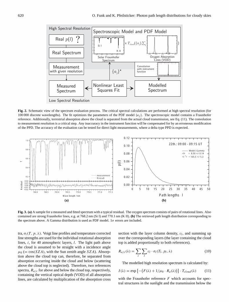
5 Spectrum analysis and instrumental setup
The transmissions for a wide range of absorption strengthsT (α), i.e. the Laplace transform of the path length dis-tribution (Eq. 3), can be measured by oxygen A-bandspectroscopy (e.g. Pfeilsticker et al., 1998; Harrison andMin, 1997). The main advantages of the oxygen A-band(b16+g ← X36−g , 759–775 nm) are the lack of interferencewith other atmospheric absorbers (as oxygen is the only ab-
sorber in this spectral range) and the constant oxygen mixingratio. Additionally, the absorption characteristics of oxygenare known very accurately. The key problem in the spectrumevaluation is the insufficient resolution of the spectrograph.Since the true transmissions are required for the analysis ofEq. (3), the measured spectrum must be corrected for resolu-tion effects. Pfeilsticker et al. (1998) corrected the transmis-sions for the centers of a set of A-band absorption lines byusing a curve of growth measured for direct light. However,the curve of growth is dependent on the path length distribu-tion, since it modifies the line shapes of the absorption lines.Therefore, this method introduces a systematical error. Therefined method presented here solves this problem by firstmodelling the true absorption line shapes for the current pathlength distribution at high spectral resolution (5×10⁻² pm)and then converting the whole modelled spectrum to the mea-surement resolution by convolution with the instrument func-tion (see Fig. (4). The spectroscopic model uses spectro-scopic data from Ritter and Wilkerson (1987) and Gamacheet al. (1998), and radio sonde atmospheric pressure and tem-perature profiles,p andT , to calculate cross section spec-
620 O. Funk and K. Pfeilsticker: Photon path length distributions for cloudy skies
Fig. 2. Schematic view of the spectrum evaluation process. The critical spectral calculations are performed at high spectral resolution (for100 000 discrete wavelengths). The fit optimizes the parameters of the PDF model{aj }. The spectroscopic model contains a Fraunhoferreference. Additionally, terrestrial absorption above the cloud is separated from the actual cloud transmission, see Eq. (11). The convolutionto measurement resolution is a critical step. Any inaccuracy in the instrument function will be compensated for by an erroneous modificationof the PPD. The accuracy of the evaluation can be tested for direct light measurements, where a delta type PPD is expected.
Fig. 3. (a)A sample for a measured and fitted spectrum with a typical residual. The oxygen spectrum consists of pairs of rotational lines. Alsocontained are strong Fraunhofer lines, e.g. at 768.2 nm (Si I) and 770.1 nm (K II).(b) The retrieved path length distribution corresponding tothe spectrum above. A Gamma distribution is used as PDF model. 1σ errors are included.
tra,σi(T , p, λ). Voigt line profiles and temperature correctedline strengths are used for the individual rotational absorptionlines, i, for 40 atmospheric layers,l. The light path abovethe cloud is assumed to be straight with a incidence angleµ0 (= cos(SZA), with the Sun zenith angleSZA). Absorp-tion above the cloud top can, therefore, be separated fromabsorption occurring inside the cloud and below (scatteringabove the cloud top is neglected). Therefore, two referencesspectra,Ra/c for above and below the cloud top, respectively,containing the vertical optical depth (VOD) of all absorptionlines, are calculated by multiplication of the absorption cross
section with the layer column density,cl , and summing upover the corresponding layers (the layer containing the cloudtop is added proportionally to both references).
Ra/c(λ) =∑i
∑l
cl · σi(Tl, pl, λ) (10)
The modelled high resolution spectrum is calculated by:
I (λ) = exp{−
(F(λ)+ 1/µ0 · Ra(λ)
)}· Tcloud(λ) (11)
with the Fraunhofer referenceF which accounts for spec-tral structures in the sunlight and the transmission below the
O. Funk and K. Pfeilsticker: Photon path length distributions for cloudy skies 621
20 10 0 -10 -20 -30 -40 -50
14 October 1998CLARE 98Chilbolton, UK
Start: 13:59 UTC
dBZe (HH) GKSS W-band Radar
HE
IGH
T A
GL
(km
)
TIME (UTC)
14h05m 14h10m 14h15m
1 2 3 4 5 6 7 8 91011121314
1 2 3 4 50
1
2
3
Model: Gamma<l> = 1.78 +/- 0.36
<l2> = 4.34 +/- 2.0
p(l)
Path lengths l
14th.: 14:00 - 14:15 UT
(a) (b)
Fig. 4. (a)Cloud structure (backscatter ratio) measured by the 94 GHz cloud Radar MIRACLE.(b) A high cirrus cloud layer reduces themean photon path length compared to the clear sky, due to an increased probability for a nearly vertical path after a scattering event in highaltitudes.
cloud top,Tcloud , calculated using a discrete and correctlynormalized PDF modelp(li) with parameters{aj }:
Tcloud(λ) =1
N
npdf∑i=1
p(li, {aj }) exp{−li · Rc(λ)} . (12)
This modelled spectrum is then convoluted (?) with theinstrument function,fλ, and fitted to the measured spectrum,Imeas , using a modified Levenberg Marquard method for theleast-squares fit, (More et al., 1980), with the{aj } being thefree parameters.
I (λ, {aj }) ? fλLSF= Imeas(λ) → {aj }
∗ (13)
In the retrieved PDF the photon path lengths are given inunits of the cloud top height.
The instrumental setup is equivalent to the setup describedin Pfeilsticker et al. (1998). The sky light collected by azenith pointing telescope (field of view 0.86◦) is conductedby a quartz fiber via an optical band pass filter (771.4 nm,FWHM of 11.2 nm) into an Echelle monochromator (ModelMPP1, Aerolaser, focal length 1250 mm, numerical aperturef/15.3, grating: blaze angle 65◦, 100 gr/mm). The spectralresolution is 19.4 pm. The spectrum is recorded by a photodiode array detector (1024 channels, 25µm, channel disper-sion 4.1 pm), digitized (ADC resolution 16 bit) and storedon a PC. The raw spectrum is corrected for electronic offset,photo diode dark current and the overall spectral sensitivity.For further details on the measurements and evaluation, referto Funk (2000).
Due to the low intensity of the zenith scattered light andthe high spectral resolution of these measurements, the spec-tra must be integrated for typically 900 seconds. (This is
mainly a constraint of the low gain of the PDA detector used,since modern CCD detectors are much more sensitive. How-ever, the problem of low photon statistics remains.) This in-tegration corresponds to an intensity-weighted temporal av-eraging. Under the assumption of slow changes in the cloudstructure, the temporal averaging corresponds to a spatial av-eraging over a scale, determined by the integration time andthe drift speed of the clouds (ergodicity). Additionally, thediffusion inside the cloud leads to spatial averaging. Thesize of this radiative smoothing scale (Marshak et al., 1995;Savigny et al., 1999) is strongly dependent on the degree ofinhomogeneity. In the case of a single, homogeneous cloudlayer, the mean lateral displacement for transmission is equalto the layer thickness. More details on scales are discussedin Pfeilsticker (1999).
A measured spectrum, together with the result of the eval-uation and the retrieved path length distribution, is shown inFig. 3.
6 Cloud optical thickness
A second result of the above fit is the high resolution trans-mission spectrumTcloud(λ, {aj }∗). These transmissions canbe compared to those resulting from radiative transfer modelcalculations. Here the 1-D discrete ordinate RT model DIS-ORT (Stamnes et al., 1988) is used. The absorption proper-ties (σa) are constant and known. The scattering propertiescan be parameterized using the cloud optical thicknessτc, de-fined as the vertical integral of the scattering coefficientαs ,τc =
∫Hcαs dz, or asτc = Hc/λc, with the mean free path
inside the cloudλc and the cloud geometrical thicknessHc.
622 O. Funk and K. Pfeilsticker: Photon path length distributions for cloudy skies
-4.0 -3.0 -2.0 -1.0 0.0 1.0
22 October 1998CLARE 98Chilbolton, UK
Start: 09:19 UTC
Velocity (m/s) GKSS W-band Radar H
EIG
HT
AG
L (
km)
TIME (UTC)
09h25m 09h30m 09h35m 09h40m
1 2 3 4 5 6 7 8 9101112
20 10 0 -10 -20 -30 -40 -50
22 October 1998CLARE 98Chilbolton, UK
Start: 09:19 UTC
dBZe (HH) GKSS W-band Radar
HE
IGH
T A
GL
(km
)
TIME (UTC)
09h25m 09h30m 09h35m 09h40m
1 2 3 4 5 6 7 8 9101112
(a)
0 5 10 15 20 25 30 35 40 45 500.00
0.02
0.04
0.06
0.08
Model: Gamma<l> = 11.6 +/- 0.14
<l2> = 217.5 +/- 9.4
p(l)
Path lengths l
22th.: 09:31 - 09:46 UT
(b)
Fig. 5. (a), (c)Cloud structure (backscatter ratio) and vertical (Doppler) velocity measured by the 94 GHz cloud Radar MIRACLE. In thefirst Case (a) two pronounced layers can be found, while no clear layer borders are present in the second Case (c). In this case the cloud fillsthe sky between 300 m and 10 km and is internally more inhomogeneous.(b), (d) The retrieved PPD for the two cases reflect the differencein cloud structure. The distribution is broader for the first Case (b), as expected for two cloud layers, see Fig. 6 (Fig. 5 continues next page).
All other scattering properties are given in Table 1. Severalcloud layers can be included. The free model parameters arethe cloud optical thicknesses{τc,i} of these layers. A least-squares fit is used to find the{τc,i}∗ for which the transmis-sions from the RT model agree best with those gained fromthe PPD retrieval.
Tcloud(λ)LSF= T RT (λ, {τc}, σa) → {τc}
∗ (14)
Since the transmission at a certain wavelength is only de-pending on the path length distribution, this method yieldsthe equivalent optical thicknesses of homogeneous cloud lay-ers which result in a similar path length distribution. Thisoptical thickness can be compared with theτc gained from
liquid water path (LWP) measurements, using the effectiveradiusre for the corresponding cloud type (Slingo, 1989):
τc =3
2
LWP
re. (15)
7 Results
The measurements presented here were conducted duringthe cloud RADAR intercomparison campaign CLARE’98 atChilbolton, Hampshire, UK (51.13◦N, 1.43◦W, 84 m) duringOctober 1998. The collocated zenith viewing 94 GHz cloud
O. Funk and K. Pfeilsticker: Photon path length distributions for cloudy skies 623
20 10 0 -10 -20 -30 -40 -50
22 October 1998CLARE 98Chilbolton, UK
Start: 09:41 UTC
dBZe (HH) GKSS W-band Radar H
EIG
HT
AG
L (
km)
TIME (UTC)
09h45m 09h50m 09h55m 10h00m
1 2 3 4 5 6 7 8 9101112
-4.0 -3.0 -2.0 -1.0 0.0 1.0
22 October 1998CLARE 98Chilbolton, UK
Start: 09:41 UTC
Velocity (m/s) GKSS W-band Radar
HE
IGH
T A
GL
(km
)
TIME (UTC)
09h45m 09h50m 09h55m 10h00m
1 2 3 4 5 6 7 8 9
101112
(c)
0 10 20 30 40 500.00
0.02
0.04
0.06
0.08
Model: Gamma<l> = 11.74 +/- 0.24
<l2> = 199 +/- 13
p(l)
Path lengths l
22th.: 09:46 - 10:01 UT
(d)
Fig. 5. ... continues
radar MIRACLE operated by GKSS (Geesthacht, Germany)recorded detailed information about the cloud structure. Ofparticular interest for this study is the vertical distribution ofthe cloud layers and the cloud top height. The cloud base ismeasured accurately by a ceilometer. Additionally, data col-lected by a microwave radiometer operated by TUE (Eind-hoven, Netherlands) was used to retrieve the cloud liquidwater path. The sum of these complementary measurementsform a good data set to study the effect of cloud structureon the radiative transfer. Some exemplary cloud cases arepresented here.
Figure 4 shows the result for a relatively thin cirrus cloudlayer in about 8 km height. A high cloud layer is expectedto reduce the mean photon path lengths for zenith viewinggeometry, since the probability for a vertical path is largely
increased. The direct light air mass factor (AMF= 1/µ0) is2.4 for this measurement, and the retrieved mean path lengthis 1.8 (always in units of the vertical path), which agrees withthe expectation. The exact form of the PPD is determined bythe PDF model; however, a maximum probability for nearlyvertical paths is reasonable for this case.
Figure 5 shows the cloud structures and retrieved PPDs fortwo subsequent measurements. During the first measurement(09:31–09:46 UT), two separated extended cloud layers areobserved. The weak structure between these layers resultsfrom precipitation originating from the upper layer. Sincethe larger precipitating drops cause a superproportional largebackscatter signal (the backscatter ratio depends on the par-ticle diameterd to the sixthd6), the radar signal betweenthe cloud layers around 09:35 UT is presumably caused by
624 O. Funk and K. Pfeilsticker: Photon path length distributions for cloudy skies
0 10 20 30 40 500
50
100
150
200
250
300
350
Fre
quen
cy
Pathlength
Case 1 (09:31) Case 2 (09:46)
Fig. 6. Monte Carlo path length histograms calculated for the twomeasurements given in Fig. 5, using the cloud optical thicknessesfrom Table 3. The distributions show the same qualitative behavioras observed. The distribution is broader for the case of separatedlayers (1) compare to the case of one compact layer (2).
optically thin rain, Fig. 5a. During the second measurement(09:46–10:01 UT), heavy precipitation falls out of the upperlayer, closing the gap between the two layers. An inhomoge-neous mixture of cloud and rain emerges from the cloud baseat 300 m (from ceilometer) to the cloud top at 9000 m withno clear borders, Fig. 5c. This transition from a two-layerstack to a single extended layer is reflected by the retrievedPPDs. While the mean path length remains nearly constant〈l〉 = 11.6, the distribution is wider in the first case and moreconcentrated around the mean for the second case. This isalso seen in lower second moments of〈l2〉 = 217 for the firstdistributions compared to〈l2〉 = 199 for the second case.The broadening of the distribution for two separated cloudlayers can be explained by reflections between the cloud lay-ers which dominate the radiative transfer in this case, whilefor a compact layer the photon path lengths are more cen-tered around the diffusion mean path length.
This behavior is verified by Monte Carlo simulations forthese two cases. Therefore, the optical thickness of the cloudlayers was derived using the method described in Sect. 6.The results are displayed in the left half of Table 3, markedasτc,RT . Total cloud optical thicknesses of 144 and 197 arefound for measurement 1 and 2, respectively. These opticalthicknesses are used in the MC model described in Sect. 4,to generate path length histograms, Fig. 6. The measuredshapes of the PPDs are qualitatively well reproduced by theMC model.
Finally, the retrieved cloud optical thicknesses are com-pared to the LWP data from the MW measurements. Themeasured mean LWPs for the two cases are 0.35 mm and0.65 mm, see Table 3. Using Eq. (15) and the retrieved cloudoptical thicknesses, this results in reasonable values for thevertically averaged effective radii of 3.65µm and 4.96µmfor Cases 1 and 2, respectively. Using the geometrical thick-ness and LWP andre for standard cloud types reported byStephens (1979) (Sc1, St1, St2), the agreement with the re-
Table 3. Results for the cloud optical thickness from the fit of thetransmissions with the 1-D RT model (left half) and from the LWPmeasurements (right half). For the RT model, asymmetry factors of0.85 and 0.7 were used for the lower and upper layer, respectively
trieved optical thicknesses is not as good. However, this isnot surprising given the variability of these parameters evenfor the same cloud type and the degree of inhomogeneityfound, especially in the second case.
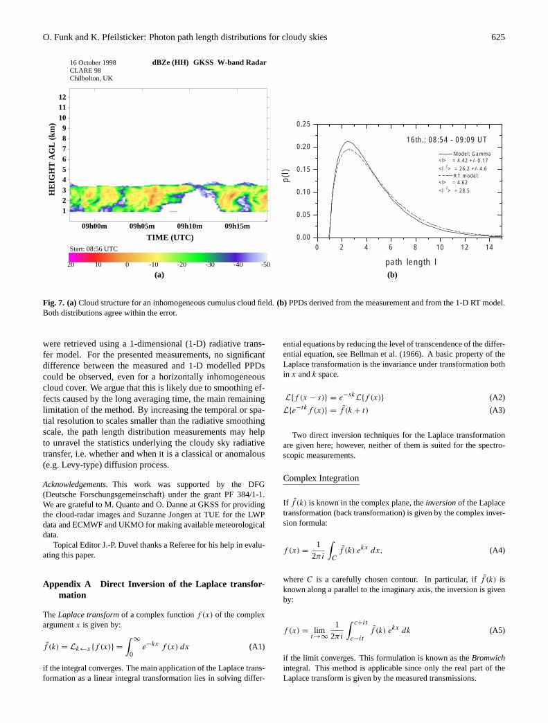
As a last case, Fig. 7 shows a single low level cumuluscloud layer between 300 m and 3300 m. Typically for theseclouds is that the cloud base and top are well-defined, whilethere is a great degree of internal inhomogeneity and largegaps. The retrieved optical thickness isτc = 44.7 ± 2.0.The path length distribution resulting from the transmissionsfrom the RT model is included in Fig. 7, together with theretrieved PPD. Both the PPDs agree within the error. A dif-ferent shape, resulting from the plane-parallel model and themeasurement, is not found for this case (within the errors), inagreement with findings reported by Portmann et al. (2001).
The mean LWP from the microwave radiometer is approx.0.3 mm. For a mean optical depth of 44.7, this LWP trans-lates into a mean effective radius of 10µm, which is a typ-ical value for stratocumulus or cumulus clouds (Sc 2/Cu,Stephens, 1979). However, the mean free path for the wholelayer is 67 m. This value is much longer than the typicalmean free path of 10–15 m for Sc 2 or Cu clouds. This en-hanced mean free path might be explained by the inhomoge-neous distribution of the liquid water content. For this casethe cloud inhomogeneity only seems to prolong the meanfree path, but has apparently no effect on the shape of thePPD.
8 Conclusions
With the presented improved method for oxygen A-bandPPD measurements, a validated tool for the investigation ofcloudy sky radiative transfer statistics is at hand. The ana-lyzed cases already provide a taste of the new informationthat can be obtained, and the analysis which is possible pro-vided an extensive data set, such as for CLARE’98. The ef-fect of vertical cloud inhomogeneities on the path length dis-tribution could be measured and reproduced qualitatively byMonte Carlo RT model calculations. Effective cloud opticalthicknesses for equivalent horizontally homogeneous layers
O. Funk and K. Pfeilsticker: Photon path length distributions for cloudy skies 625
20 10 0 -10 -20 -30 -40 -50
16 October 1998CLARE 98Chilbolton, UK
Start: 08:56 UTC
dBZe (HH) GKSS W-band Radar H
EIG
HT
AG
L (
km)
TIME (UTC)
09h00m 09h05m 09h10m 09h15m
1 2 3 4 5 6 7 8 9101112
0 2 4 6 8 10 12 140.00
0.05
0.10
0.15
0.20
0.25
16th.: 08:54 - 09:09 UT
p(l)
path length l
Model: Gamma<l> = 4.42 +/- 0.17
<l2> = 26.2 +/- 4.6
RT model:<l> = 4.62
<l2> = 28.5
(a) (b)
Fig. 7. (a)Cloud structure for an inhomogeneous cumulus cloud field.(b) PPDs derived from the measurement and from the 1-D RT model.Both distributions agree within the error.
were retrieved using a 1-dimensional (1-D) radiative trans-fer model. For the presented measurements, no significantdifference between the measured and 1-D modelled PPDscould be observed, even for a horizontally inhomogeneouscloud cover. We argue that this is likely due to smoothing ef-fects caused by the long averaging time, the main remaininglimitation of the method. By increasing the temporal or spa-tial resolution to scales smaller than the radiative smoothingscale, the path length distribution measurements may helpto unravel the statistics underlying the cloudy sky radiativetransfer, i.e. whether and when it is a classical or anomalous(e.g. Levy-type) diffusion process.
Acknowledgements.This work was supported by the DFG(Deutsche Forschungsgemeinschaft) under the grant PF 384/1-1.We are grateful to M. Quante and O. Danne at GKSS for providingthe cloud-radar images and Suzanne Jongen at TUE for the LWPdata and ECMWF and UKMO for making available meteorologicaldata.
Topical Editor J.-P. Duvel thanks a Referee for his help in evalu-ating this paper.
Appendix A Direct Inversion of the Laplace transfor-mation
TheLaplace transformof a complex functionf (x) of the complexargumentx is given by:
f (k) = Lk←x{f (x)} =∫∞
0e−kx f (x) dx (A1)
if the integral converges. The main application of the Laplace trans-formation as a linear integral transformation lies in solving differ-
ential equations by reducing the level of transcendence of the differ-ential equation, see Bellman et al. (1966). A basic property of theLaplace transformation is the invariance under transformation bothin x andk space.
L{f (x − s)} = e−skL{f (x)} (A2)
L{e−tkf (x)} = f (k + t) (A3)
Two direct inversion techniques for the Laplace transformationare given here; however, neither of them is suited for the spectro-scopic measurements.
Complex Integration
If f (k) is known in the complex plane, theinversionof the Laplacetransformation (back transformation) is given by the complex inver-sion formula:
f (x) =1
2πi
∫Cf (k) ekx dx, (A4)
whereC is a carefully chosen contour. In particular, iff (k) isknown along a parallel to the imaginary axis, the inversion is givenby:
f (x) = limt→∞
1
2πi
∫ c+it
c−itf (k) ekx dk (A5)
if the limit converges. This formulation is known as theBromwichintegral. This method is applicable since only the real part of theLaplace transform is given by the measured transmissions.
626 O. Funk and K. Pfeilsticker: Photon path length distributions for cloudy skies
Using the Characteristic Function
The Characteristic Functionχ of p(l) is given by Fourier trans-form of p(l). By expansion of the exponential functionχ can beexpressed by all momentsmj of p(l)
χ(k) =
∫∞
0p(l)e−ikldl =
∑j
(−ik)j
j !mj (A6)
with mj =
∫∞
0p(α)ljdl . (A7)
p(l) is then given by the inverse Fourier transform:
p(l) =1
2π
∫∞
0χ(k) eikl dk. (A8)
The momentsmj can be found by expanding the exponential func-tion in Eq. (3):
T (α) =
∫∞
0p(l)
∑j
(−α)j
j !lj
dl =∑j
(−α)j
j !mj . (A9)
For weak absorbers, i.e.α < l >� 1, the first order approximationyields the well-known relation:
Tα<l>�1 ≈ 1− α < l > and (A10)
τ = − ln T ≈ α < l > (A11)
This method uses the close relationship between Laplace trans-formation and Fourier transformation. Unfortunately, the inverseFourier transformation is difficult to apply, since all moments arerequired. The complexe function is converging very slowly withlarge oscillations for arguments> 1.
References
AGU: Proceedings of the Chapmann Conference on AtmosphericAbsorption of Solar Radiation, American Geophysical Union,Estes Park, Colorado, on August 13-17, 2001.
Bellman, R., Kalaba, R. E., and Lockett, J. A.: Numerical Inversionof the Laplace Transform: Applications to Biology, Economics,Engineering, and Physics, American Elsevier Publishing, NewYork, 1966.
Davis, A., Marshak, A., Wiscombe, W. J., and Cahalan, R. F.:Scale-invariance of liquid water distributions in marine stratocu-mulus, i - spectral properties and stationarity issues, J. Atmos.Sci., 53, 1538–1558, 1996.
Davis, A. and Marshak, A.: Levy kinetics in slab geometry: Scalingof transmission probability, in: Fractal Frontiers, (Eds) Novak,M. M. and Dewey, T. G., pp. 63–72, World Sci., N.J., 1998.
Funk, O.: Photon Pathlengths Distributions for Cloudy Skies –Oxygen A-Band Measurements and Radiative Transfer ModelCalculations, Ph.D. thesis, Institut fur Umweltphysik, Ruprecht-Karls-Universitat Heidelberg, 2000.
Gamache, R. R., Goldman, A., and Rothman, L. S.: Improved spec-tral parameters for the three most abundant isotopomers of theoxygen molecule, J. Quant. Spectr. Rad. Trans., 59, 495–509,1998.
Harrison, L. and Min, Q.-L.: Photon path length distributions in
cloudy atmospheres from ground-based high resolution O2 a-band spectroscopy, in: IRS’96:Current Problems in AtmosphericRadiation, (Eds) Smith, W. L. and Stamnes, P., A. Deepak,Hampton, Va, 1997.
Isaacs, R. G., Wang, W.-C., Worsham, R. D., and Goldberg, S.:Multiple scattering lowtran and fascode models, Appl. Opt., 26,1272–1281, 1987.
Marshak, A., Davis, A., Wiscombe, W., and Cahalan, R.: Radia-tive smoothing in fractal clouds, J. Geophys. Res., 100, 26 247–26 261, 1995.
Min, Q., Harrison, L. C., and Clothiaux, E. E.; Joint statistics ofphoton path length and cloud optical depth: Case studies, J. Geo-phys. Res., 106, 7375–7385, 2001.
More, J., Garbow, B., and Hillstrom, K.: User guide for MINPACK-1, Argonne National Labs Report ANL-80-74, Argonne, Illinois,1980.
Nicolet, M.: On the molecular scattering in the terrestrial atmo-sphere: An empirical formula for its calculation in the homo-sphere, Planet. Space Sci., 32, 1467–1468, 1984.
Pfeilsticker, K.: First geometrical path lengths probability den-sity function derivation of the skylight from spectroscopicallyhighly resolving oxygen aband observations 2. derivation of thelevyindex for the skylight transmitted by midlatitude clouds, J.Geophys. Res., 104, 4101–4116, 1999.
Pfeilsticker, K., Erle, F., Funk, O., Veitel, H., and Platt, U.: Firstgeometrical path lengths probability density function derivationof the skylight from spectroscopically highly resolving oxy-gen aband observations 1. measurement technique, atmosphericobservations, and model calculations, J. Geophys. Res., 103,11 483–11 504, 1998.
Portmann, R. W., Solomon, S., Sanders, R. W., and Daniel, J. S.:Cloud modulation of zenith sky oxygen photon path lengths overboulder, colorado: Measurements vs. model, J. Geophys. Res.,106, 1139–1155, 2001.
Ritter, K. J. and Wilkerson, T. D.: High resolution spectroscopy ofthe oxygen A-Band, J. Molec. Spectrosc., 121, 1–19, 1987.
Savigny, C. v., Funk, O., Platt, U., and Pfeilsticker, K.: Radiativesmoothing in zenith-scattered skylight transmitted through opti-cally thick clouds to the ground, Geophys. Res. Lett., 26, 2949–2952, 1999.
Slingo, A.: A gcm parameterization for the shortwave radiativeproperties of water clouds, J. Atm. Sci., 46, 1419–1427, 1989.
Stamnes, K., Tsay, S.-C., Wiscombe, W., and Jayaweera, K.: Nu-merically stable algorithm for discrete-ordinate-method radiativetransfer in multiple scattering and emitting layered media, Ap-plied Optics, 27, 2502–2509, 1988.
Stephens, G. L.: Optical Properties of Eight Water Cloud Types,CSIRO, tech. paper no. 36 edn., 1979.
Stephens, G. L. and Tsay, S.-C.: On the cloud absorption anomaly,Q. J. R. Meteorol. Soc., 116, 671–704, 1990.
Van de Hulst, H. C.: Multiple Light Scattering, Tables, Formulasand Applications, Volume 1 and 2, Academic Press, London,1980.
Wild, M., Ohmura, A., Gilgen, H., and Roecker, E.: Validation ofgeneral circulation model radiative fluxes using surface observa-tions, J. Climate, 8, 1309–1324, 1995.
Wild, M., Ohmura, A., Gilgen, H., Roecker, E., and Giogetta,M.: Improved representation of surface and atmospheric radia-tion budgets in the ECHAM4 general circulation model, MPI-Meteorologie, Hamburg, report no. 200 edn., 1996.