GEOPHYSICAL MAPPING OF SALTWATER

INTRUSION IN EVERGLADES NATIONAL PARKDavid V. FittermanMaria Deszcz-Pan

U.S. Geological SurveyBox 25046 MS 964Denver, CO 80225

Phone: 303-236-1382FAX: 303-236-1409

e-mail: fitter@musette.cr.usgs.gov

Keywords: saltwater intrusion, airborne geophysics, borehole geophysics,electromagnetics, time-domain electromagnetic, induction logs, specificconductance, water quality, monitoring wells

1. ABSTRACT

The mapping of saltwater intrusion in coastal aquifers has traditionally reliedupon observation wells and collection of water samples. This approach may missimportant hydrologic features related to saltwater intrusion in areas where access isdifficult and wells are widely spaced, such as the Everglades. To map saltwaterintrusion in Everglades National Park, a different approach has been used. We haverelied heavily on helicopter electromagnetic (HEM) measurements to map lateralvariations of electrical resistivity, which are directly related to water quality. The HEMdata are inverted to provide a three-dimensional resistivity model of the subsurface.Borehole geophysical and water quality measurements made in a selected set ofobservations wells are used to determine the relation between formation resistivityand specific conductance of pore water. Applying this relation to the 3-D HEMresistivity model produces an estimated water-quality model. This model providesconstraints for variable density, ground-water models of the area. Time-domainelectromagnetic (TEM) soundings have also be used to map saltwater intrusion.Because of the high density of HEM sampling (a measurement point every 10 metersalong flight lines) models with a cell size of 100 meters on a side are possible,revealing features which could not be recognized from either the TEM or theobservation wells alone. The very detailed resistivity maps show the extent ofsaltwater intrusion and the effect of former and present canals and roadbeds. TheHEM survey provides a means of quickly obtaining a synoptic picture of saltwaterintrusion, which also serves as a baseline for monitoring the effects of Evergladesrestoration activities.

2. INTRODUCTION

The Everglades ecosystem encompasses a large area in south Floridaextending from south of Orlando to Florida Bay, a distance of over 350 km (Figure 1).Surface-water flows tie these location together starting from the Kissimmee Riverdrainage, which is located north of Lake Okeechobee. Water from the lake drains intothe Everglades and then through Everglades National Park to Florida Bay. Thebuilding of canals and levees in south Florida over the past century has severelymodified the pre-development conditions producing major changes in the ecosystem(Lodge, 1994). As a result of increased understanding of the importance of theecosystem on water supplies and the economy of south Florida, federal, state, andlocal governments have been working to reverse some of the adverse effects ofdevelopment on the Everglades. Restoration activities are aimed at understandingwhich factors influence the ecosystem, and how modification of water flows to moreclosely resemble pre-development conditions can improve the viability of theecosystem while maintaining drinking water supplies and adequate levels of floodprotection for developed areas.

One part of the restoration effort involves mapping salt-water intrusion inEverglades National Park (ENP). This information is needed to develop ground-waterflow models (Langevin, 1999; Swain, 1999), for use in geochemical studies ofground-water/surface-water interactions (Harvey et al., 1999), and to compare withreconstructions of historic saltwater intrusion based on plant and paleontologicalstudies (Brewster-Wingard et al., 1999; Willard et al., 1999). Figure 1 shows a locationmap of the study area which encompasses much of the southern tip of Florida.

Saltwater intrusion in coastal aquifers has traditionally been studied usingobservations wells and water samples. The use of monitoring wells has limited utilityin the Florida Everglades where most of the surface is covered by 10-80 cm or moreof water, and there are few roads. Another disadvantage of using wells to mapsaltwater intrusion is that lateral resolution is limited by well spacing, which in turn iscontrolled by access and economic issues. As a result, subtle features related tochanges in geology or human activity are difficult to identify. More recently inductionloggers have been used to map the freshwater/saltwater interface (FWSWI)(Sonenshein, 1997).

One approach to address the problem of limited ground access is to useairborne geophysical methods to map resistivity as a function of depth along flightlines. Because the bulk resistivity of geologic formations is highly dependent uponpore-water salinity, geophysical data can give an indirect measure of water quality.There are a number of airborne geophysical techniques that can be employed for thispurpose (Palacky, 1986; Fitterman, 1990). In this paper we describe our experience inusing helicopter electromagnetic (HEM) surveys and other ground based methods tomap saltwater intrusion in Everglades National Park.

3. HYDROGEOLOGIC SETTING

The flow of surface water through ENP come from Shark River Slough andTaylor Slough. Shark River Slough drains into the many tidal rivers flowing to the Gulfof Mexico on the southwestern portion of the study area. Taylor Slough flowssouthward toward Florida Bay, but it is essentially blocked by the slight elevation risealong the coast called the Buttonwood Embankment. As will be shown, these differentflow regimes affect the pattern of saltwater intrusion.

Ground-water flow in our study area is controlled by the general hydrogeologicframework of Dade County, which is described by Fish and Stewart (1991). Threedistinct zones characterize the salient features of the hydrogeology: the surficialaquifer, the intermediate confining unit, and the Floridan aquifer system. Of thesezones, only the surficial aquifer is of interest to ecosystem studies because of itsinteraction with surface-water flows. The surficial aquifer is composed of the Biscayneaquifer, a semiconfining unit, the Gray limestone aquifer, and the lower clastic unit ofthe Tamiami Formation. The Biscayne aquifer contains high permeability (>1000 ft/d)limestone and calcareous sand units. It ranges in thickness from 0 to 80 ft (0-24 m)thick and increases in thickness toward the east.

4. ELECTROMAGNETIC TECHNIQUES

Electromagnetic geophysical techniques were originally developed for mineralexploration, specifically the detection of massive metallic conductors in resistive hostrock, such as found in the Canadian Shield. Because this terrain is often difficult totraverse, airborne methods were developed as early as the 1940’s to aid exploration.Over the years many ground-based and airborne geophysical methods have beendeveloped and refined for mineral exploration. The use of electromagnetic techniquesfor hydrologic studies is relatively new; there has been steady growth in their use overthe last decade. Sengpiel (1983) shows the use of helicopter electromagnetic surveysfor several ground-water exploration problems, including the mapping of saltwaterintrusion on an island. Fitterman and Hoekstra (1984) applied the transientelectromagnetic (TEM) sounding technique to the mapping of naturally occurring brinecontamination in central Michigan. Stewart and Gay (1986) used TEM soundings tomap saltwater intrusion in south Florida. Yang et al. (1999) used both TEM and DCresistivity soundings to map saltwater intrusion in Tawain.

A complete description of the various electromagnetic techniques is beyond thescope of this paper. Very complete descriptions of these methods can be found inKeller and Frischknecht (1966), Nabighian (1988, 1991), Fitterman and Stewart(1986), and McNeill (1990). Suffice it say that all of the techniques used in this studyrely upon time-varying magnetic fields from a transmitter to induce electrical currentsinto the ground. The flow of these currents is controlled by the electrical conductivity ofthe ground. More conductive zones tend to let the induced currents flow unimpeded,while less conductive zones impede the current flow. The induced currents in theground produce a secondary magnetic field which is recorded by a receiver coil.

Analysis of the received signals determines how conductivity (or its reciprocal,resistivity) varies with depth and position.

4.1 Helicopter Electromagnetic Surveying

Helicopter electromagnetic (HEM) surveys make use of a system of transmitterand receiver coils housed in a torpedo-shaped tube called a bird. The bird is typically10-m long and slung 30 m below the helicopter (see Figure 2). During surveying thebird is flown 30 m above the land surface. Using five different frequency-coil-paircombinations, the electromagnetic response is measured every 0.2 s resulting in ameasurement point about every 10 m along flight lines. Flight lines are typically 400 mapart. Such a high density of sampling is not economically or logistically feasible withground-based geophysical measurements or wells.

The electromagnetic response is measured as a function of frequency.Decreasing the frequency increases the depth of exploration. The electromagneticresponse consists of two parts, one which is in phase with the transmitted signal andthe other which is out of phase (quadrature component) with respect to thetransmitted signal. The response is measured in parts per million of the transmittedsignal and converted to an apparent resistivity to facilitate comparison of data fromdifferent locations. Apparent resistivity is the resistivity of a homogeneous half-spacerequired to produce the measured response. Keep in mind that the response wasmeasured over a heterogeneous earth, hence the use of the term apparent. Anapparent resistivity is computed for each frequency.

An apparent resistivity map alone provides no depth information, however, bycomparison of maps made using different transmitter frequencies an idea of howresistivity varies with depth can be formed. To determine true resistivity variation withdepth the data must be modeled.

Modeling entails taking data from a measurement point, consisting of theelectromagnetic response at several frequencies, and estimating the parameters of alayered-earth, resistivity-depth model that would produce the measured response.This process is called inversion and makes use of nonlinear parameter estimationtechniques (Inman, 1975; Deszcz-Pan et al., 1998; Ellis, 1998). Typically parametersfor two-, and sometimes, three-layer models can be estimated. Noise in the data,however, often produces large misfits between the measured and observedelectromagnetic response, requiring the winnowing of some of the inversion models.Because the geology and hydrologic conditions vary slowly from point to point in theEverglades (Fish and Stewart, 1991), we are justified in using 1-D models. Thenumerous resistivity-depth models are sliced at specified depths to produceresistivity-depth-slice maps (see Figure 2).

4.2 Transient Electromagnetic Soundings

Unlike the HEM method which has the transmitter on at all times, the transientelectromagnetic (TEM) sounding method uses the transition from a steady to zero

transmitter current to induce current in the ground. The ground response is measuredduring the transmitter off-time. We employed a 40-m by 40-m transmitter loop with thereceiver coil located at the center of the transmitter loop. The data are converted toapparent resistivity before modeling. Layered-earth model parameters aredetermined using commercially available nonlinear least-squares inversion software.Because of the large number of data points (typically 25-35) compared to the 10 foreach HEM measurement, model parameter estimates are more reliable for the TEMdata than the HEM data. The TEM method also has the ability to probe to greaterdepths than the HEM method. From these data we were able to locate the FWSWI, aswell as the depth to the base of the Biscayne aquifer.

Using the TEM method in the Everglades required slight modification ofstandard methods as most of the soundings were made in water-covered areas.Equipment had to be floated in plastic tubs, and the transmitter wire was strung oversaw grass, while the receiver coil was stood on long legs to keep it above the water.

4.3 Induction Logs

At the few sites where we had observation wells (Figure 1), induction logs weremeasured. The induction tool uses a frequency-domain electromagnetic system todetermine the formation resistivity outside the borehole. The borehole must be casedwith non-conducting material such as PVC. Induction logs provide very detailedresistivity-depth information within the vicinity of the borehole–about 1 m radius fromthe well. This information is useful in determining the relationship between formationresistivity and pore water quality (discussed in the next section).

5. ESTIMATION OF WATER QUALITY

Electromagnetic geophysical techniques, such as those described above,provide information on formation resistivity, which depends upon pore-water resistivityand porosity (Archie, 1942; Hearst and Nelson, 1985). When dealing with saltwaterintrusion, water quality, which is a property of the pore water alone, is expressed asspecific conductance or chloride ion concentration (Hem, 1970; Freeze and Cherry,1979). If we can relate formation resistivity to pore-water specific conductance andchloride ion concentration, we can use the geophysically determined resistivity modelto estimate water quality. To do this we use induction logs to obtain formationresistivity in observation wells, and water samples pumped from wells to determinespecific conductance.

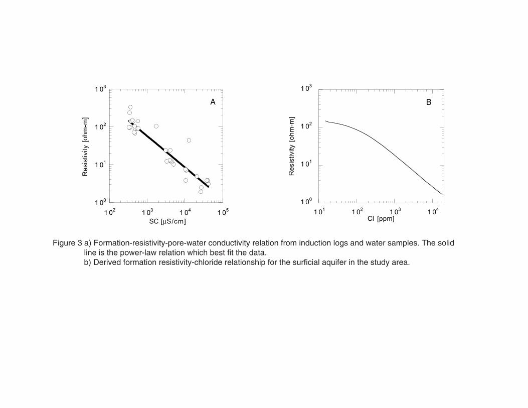
Figure 3a shows a scatter plot of formation resistivity as a function of pore-water conductivity from test wells in the study area. The data points represent averageformation resistivity over the screened interval in the well and the measuredconductivity of water produced from this interval. In some cases a down-hole waterconductivity probe was used. Most, but not all, of the points are in the Biscayneaquifer. The linear regression line allows conversion of formation resistivity to specificconductance. To express specific conductance as chloride concentration, we make

use of another empirical relationship applicable to surface and near-surface waters inDade County (A. C. Lietz, USGS Miami, written commun., 1998). The final result is thecurve in Figure 3b which shows the relationship between formation resistivity andchloride concentration. While the curve plots as a smooth line, there is an inherentuncertainty in the estimated chloride concentration due primarily to the scatter in thedata in Figure 3a. Nevertheless, the chloride concentration is probably correct towithin a factor of 2 to 5 based on the scatter in formation-resistivity-specific-conductance data. This relationship will be used to estimate chloride concentrationfrom the geophysical models.

6. GEOPHYSICAL RESULTS

6.1 HEM Data

Figure 4 shows a 56-kHz apparent resistivity map from Everglades NationalPark. Within the central part of the survey most apparent resistivity values are greaterthan 30 ohm-m with many values exceeding 75 ohm-m. In contrast, near the coast theapparent resistivities are generally less than 5 ohm-m with values below 1 ohm-m notuncommon. This dramatic variation is interpreted as being due to saltwater intrusionin the coastal areas and a fresh-water saturated aquifer further inland. Based on therelationship between formation resistivity and chloride concentration (Figure 3b), thetransition from saltwater to freshwater saturation occurs between 10 and 15 ohm-m.As we are dealing with apparent resistivity in this map, the resistivity value of thetransition is less certain. Nonetheless, the sharp gradient in the region of TaylorSlough and to the east is caused by the FWSWI. In the western portion of the surveywhere the boundary corresponds to the terminus of the tidal rivers, the transition zoneis more diffuse.

Four depth slices are shown in Figure 5 based on layered earth inversions.These particular maps where chosen because there are significant changes betweenthem. Many features related to saltwater intrusion and the impact of roads and canalson water flows can be seen in them. There is a general decrease in resistivity towardFlorida Bay in the south as a result of saltwater intrusion. In the Taylor Slough area (a)the transition between freshwater and saltwater occurs over a short distance. Thetrace of the interface on the map varies smoothly because the hydrologic conditionsdo not vary rapidly parallel to the interface. The position and shape of the interface iscontrolled by the balance between ground-water flow to the south, andevapotranspiration losses and saltwater intrusion. To the west (b), tidal rivers drainthe area and allow seawater to move inland a great distance. The result is a lessabrupt transition from fresh-water to salt-water saturated zones spread over a greaterdistance than near Taylor Slough. Parallel the interface there is more variability in thelandward extent of salt-water intrusion because of the influence of the rivers.

Several man-made structures have a significant influence on the hydrology asmanifested in the resistivity depth slices. Along the main park road (c) there is a four-fold change in resistivity from one side to the other. This feature, which extends to at

least 10-m depth, is due to the roadbed blocking the westward flow of freshwater fromTaylor Sough. Roads play an important role in controlling the flow of surface waterbecause they are typically raised 1-2 m above the water covered marshes.

Along old Ingraham Highway (d) a conductive feature is seen. This road wasconstructed between 1915 and 1919 by digging a canal along the side of the roadwayand piling up the dredged material. The resulting canal was originally open fromFlorida Bay near the town of Flamingo all the way to Royal Palm. Seawater migratedinland along this entire section of the canal. The canal was plugged in 1951. Webelieve that this low resistivity anomaly is due to seawater which remains in theaquifer.

The C-111 canal is a major drainage canal which leads to Biscayne Bay. Oneof its current functions is to provide water to the southeastern portion of EvergladesNational Park. This is accomplished through cuts in the spoil piles along the southernbank of the canal from the bend in the canal to highway U.S. 1. In the 5-m and 10-mdepth slices a resistivity high (e) is seen to the south of the canal because offreshwater recharge from the canal. This recharge produces a freshwater zone to thesouth of the main FWSWI location seen in the 10-m and 15-m depth slices. In the 15-m depth slice a cusp in the FWSWI (f) is seen where the C-111 canal crosses theinterface. This cusp is produced by water impoundment behind a moveable dam onthe canal (control structure S18C).

One issue of concern to studies of Florida Bay is whether or not there are fresh,ground-water flows to Florida Bay. The HEM results indicate that no fresh-water zoneexists south of the FWSWI (g). Based on this and other geophysical data, it is highlyunlikely that there are fresh, ground-water flows to Florida Bay.

In all of the depth slices a high resistivity zone associated with Taylor Slough(h) is seen. Taylor Slough is the major source of water to the central portion ofEverglades National Park. From the HEM interpretation this zone is seen to extend toa depth of at least 40 m.

6.2 TEM Data

The TEM sounding data from two representative locations are shown inFigure 6. (See Figure 1 for sounding locations.) Sounding EG108 is from a regionseaward of the FWSWI as determined from the HEM data, while EG111 is landward ofthe interface. Both soundings are east of Taylor Slough and south of the C-111 canal.The measured apparent resistivity is shown as a function of time after transmitter-current turn off. Also plotted is the computed apparent resistivity of the model whichbest fits the data. The apparent resistivity for sounding EG111 decreases with time,approaches a steady value near 55 ohm-m, and then decreases further at later time.Sounding EG108 has a much more dramatic decrease at early time, an easilyrecognized minimum of about 5.5 ohm-m, and a final increase in apparent resistivity.The apparent resistivities of sounding EG108 are consistently lower than those ofsounding EG111.

The model resistivities in Figure 6b confirm the general behavior of theapparent resistivity curves. At site EG111 the resistivity decreases monotonically withdepth. The thick second layer (109 m) has a resistivity of 43 ohm-m and produces thesteady value seen in the middle of the apparent resistivity curve. Sounding EG108 hasa resistivity minimum of 2.8 ohm-m between 11 m and 29 m depth which producesthe apparent resistivity minimum.

A histogram of interpreted layer resistivities for all of the TEM soundings (notshown) exhibits a natural division of interpreted layer resistivities of those less than10 ohm-m from those that are greater. This division corresponds to the transition fromfresh to saline water and provides a basis for using the TEM results to map theFWSWI.

7. DISCUSSION

Figure 7 shows the results from the three data sets used to map the FWSWI.The TEM locations have been plotted with symbols color coded to indicate if theinterpreted resistivity of the surficial aquifer is greater or less than 10 ohm-m.Resistivities less than this value are considered to be saltwater intruded. Using theTEM data a line representing the FWSWI has been interpolated between the soundinglocations. Similarly the locations of the observation wells have been color coded andplotted. Wells with specific conductances of greater than 3000 µS/cm are consideredto be saltwater intruded. A line showing the FWSWI based on the well data is alsoplotted. Last, the interpreted-resistivity, 10-m depth-slice map from the HEM data isshown. In this map the interface occurs around 10 ohm-m, which corresponds to anestimated chloride concentration of about 2100 ppm.

Comparison of the three interpretations of the FWSWI show, as expected, thatthe data set with the highest spatial sampling density, the HEM data, shows the mostdetail. The TEM derived FWSWI has pretty good agreement from the bend of the C111canal to the western limit of Taylor Slough, but becomes less detailed to the west assampling density diminishes. The well-derived FWSWI misses several majorfeatures such as the southward extent of the FWSWI in the middle of Taylor Slough,the old Ingraham Highway canal anomaly, and the effect of the tidal rivers to the west.If ground access were not an issue, a more detailed picture of the interface couldhave been obtained through the use of carefully chosen TEM soundings. However, itis unlikely that TEM soundings alone could match the detail of the HEM data. Usingwells to achieve a similar results would be very difficult if not impossible.

8. CONCLUSIONS

Ground and airborne electromagnetic methods have been shown to be aneffective method for mapping saltwater intrusion in Everglades National Park. Theresults of these surveys and well measurements are in agreement. The HEM datawith its high sampling density presents a detailed picture of saltwater intrusion that, inturn, allows identification of factors influencing the location of the FWSWI. The

interpreted resistivity maps, when combined with well log data to determine theformation-resistivity-chloride-concentration relationship, provide a means ofdeveloping a three-dimensional water quality model that can be used in ground-watermodeling studies.

Because the HEM data were collected in less than five days, the resultsessentially provide a snapshot of the entire aquifer. At present, there is no other way toobtain an equivalent synoptic picture. Equally significant, this survey can be used as abaseline against which future surveys can be compared. Such comparisons are ameans of assessing the effects of ecosystem restoration activity on saltwaterintrusion beneath the Everglades.

9. REFERENCES

Archie, G.E., 1942, The electrical resistivity log as an aid to determining somereservoir characteristics: Trans. AIME, v. 146, p. 54-62.

Brewster-Wingard, G.L, Ishman, S.E., Cronin, T.M., Willard, D.A., and Huvane, J, 1999,Historical patterns of change in the Florida Bay ecosystem [abstract], in Gerould,S., and Higer, A., eds., U.S. Geological Survey program on the south Floridaecosystem: U.S. Geological Survey Open-File Report 99-181, 4-5 p.

Deszcz-Pan, M., Fitterman, D.V., and Labson, V.F., 1998, Reduction of inversion errorsin helicopter EM data using auxiliary information: Exploration Geophysics, v. 29,p. 142-146.

Ellis, R. G. 1998, Inversion of airborne electromagnetic data: Exploration Geophysics,v. 29, p. 121-127.

Fish, J. E. and Stewart, M., 1991, Hydrogeology of the surficial aquifer system, DadeCounty, Florida: U.S. Geological Survey Water-Resources Investigations Report90-4108, 50 p.

Fitterman, D.V., ed., 1990, Developments and Applications of Modern AirborneElectromagnetic Surveys, U.S. Geological Survey Bulletin 1925, 3 plates and216 p.

Fitterman, D.V., and Hoekstra, P., 1984, Mapping of saltwater intrusion with transientelectromagnetic soundings, in Proceeding of the NWWA/EPA Conference onSurface and Borehole Geophysical Methods in Ground Water Investigations,February 7-9, 1984, San Antonio, Texas, , p. 429-454.

Fitterman, D.V., and Stewart, M.T., 1986, Transient electromagnetic sounding forgroundwater: Geophysics, v. 51, p. 995-1005.

Freeze, R.A., and Cherry, J.A., 1979, Groundwater: Englewood Cliffs, New Jersey,Prentice Hall, 604 p.

Harvey, J.W., Krupa, S.L., Choi, J., Gefvert, C., Mooney, R.H., Schuster, P.F., Bates, A.L.,King, S.A., Reddy, M.M., Orem, W.H., Krabbenhoft, D.P., and Fink, L.E., 1999,Hydrologic exchange of surface water and ground water and its relation tosurface water budgets and water quality in the Everglades [abstract], in Gerould,S., and Higer, A., eds., U.S. Geological Survey program on the south Floridaecosystem: U.S. Geological Survey Open-File Report 99-181, 36-37 p.

Hearst, J.R., and Nelson, P.H., 1985, Well logging for physical properties: New York,McGraw-Hill, 571 p.

Hem, J.D., 1970, Study and interpretation of the chemical characteristics of naturalwater (2nd ed.): U.S. Geological Survey Water-Supply Paper 1473, 363 p.

Inman, J.R., 1975, Resistivity inversion with ridge regression: Geophysics, v. 40,p. 798-817.

Keller, G.V., and Frischknecht, F.C., 1966, Electrical Methods in GeophysicalProspecting: International Series of Monographs in Electromagnetic Waves:Oxford, Pergamon, 519 p.

Langevin, C.D., 1999, Ground-water flow to Biscayne Bay [abstract], in Gerould, S.,and Higer, A., eds., U.S. Geological Survey program on the south Floridaecosystem: U.S. Geological Survey Open-File Report 99-181, 58-59 p.

Lodge, T. E., 1994, The Everglades Handbook; Understanding the Ecosystem:St. Lucie Press, 228 p.

McNeill, J.D., 1990, Use of electromagnetic methods for groundwater studies, inWard, S.H., ed., Geotechnical and environmental geophysics: Tulsa, Soc. Expl.Geophys., p. 191-218.

Nabighian, M.N., ed., 1988, Electromagnetic methods in applied geophysics: Tulsa,Soc. Expl. Geophys., v. 1, 503 p.

Nabighian, M.N., ed., 1991, Electromagnetic methods in applied geophysics: Tulsa,Soc. Expl. Geophys., v. 2, 992 p.

Palacky, G.J., ed., 1986, Airborne resistivity mapping: Geological Survey of CanadaPaper 86-22, 195 p.

Sengpiel, K.P., 1983, Resistivity depth mapping with airborne electromagnetic surveydata: Geophysics, v. 48, no. 2, p. 181-196.

Sonenshein, R.S., 1997, Delineation and extent of saltwater intrusion in the Biscayneaquifer, eastern Dade County, Florida, 1995: U.S. Geological Survey Water-Resources Investigations Report 96-4285.

Stewart, M.T., and Gay, M.C., 1986, Evaluation of transient electromagnetic soundingsfor deep detection of conductive fluids: Ground Water, v. 24, p. 351-356.

Swain, E.D., 1999, Two-dimensional simulation of flow and transport to Florida Baythrough the southern inland and coastal systems (SICS) [abstract], in Gerould,S., and Higer, A., eds., U.S. Geological Survey program on the south Floridaecosystem: U.S. Geological Survey Open-File Report 99-181, 108-109 p.

Willard, D.A., Holmes, C.W., Orem, W.H., and Weimer, L.M., 1999, Plant communitiesof Everglades: a history of the last two millennia [abstract], in Gerould, S., andHiger, A., eds., U.S. Geological Survey program on the south Florida ecosystem:U.S. Geological Survey Open-File Report 99-181, 108-109 p.

Yang, C.-H., Tong, L.-T., and Huang, C.-F., 1999, Combined application of dc and TEMto sea-water intrusion mapping: Geophysics, v. 64, p. 417-425.

0 25 km81° W

25° 30' N

25° 10' N

80° 30' W

F l o r i d a B a y

Homestead

Flamingo

US 1

river or stream

canal

road

LegendHEM survey

well

TEM sounding

C-111 Canal

IngrahamHighway

SR 9336 EG111

EG108

Taylor Sloug

h

Shark Rive

r

Slou

ghRoyal Palm

B

Figure 1 a) Map of south Florida and the historic Everglades.b) Location map showing the December 1994 HEM survey, TEM soundings, and observations wells in and near Everglades National Park used in this study. Note the location of TEM soundings EG108 and EG111.

Orlando

Tampa

Ft. Meyers

Stuart

West PalmBeach

Naples Ft. Lauderdale

Miami

LakeOkeechobee

Shark RiverSlough

Florida Bay TaylorSlough

0 50 100 miles

150 km100500

Florida Keys

Headwaters: HistoricEverglades WatershedHistoric Everglades

Atlantic Coastal Ridge

A

Kissimmee River

HistoricEverglades

N

100 1k 10k 100k-50

-25

0

25

50

75

100

Frequency (Hz)

Res

pons

e (p

pm) Inphase

Quad

Dep

th (

m)

InterpretedResistivity (ohm-m)

30

25

20

15

10

5

01k100101

Inversion

Flight Line Map Resistivity Depth-Slice Map

A D

B C

Figure 2 Schematic representation of HEM data collection and interpretation. a) Flight lines are flown along parallel lines spaced 400 m apart. b) The bird measures the inphase and quadrature electromagnetic response at several frequencies. c) The measured response is used to determine the resistivity-depth function by a process called inversion. d) The resistivity-depth functions are combined to produce an interpreted resistivity depth-slice map.

µ

A B

Figure 3 a) Formation-resistivity-pore-water conductivity relation from induction logs and water samples. The solid line is the power-law relation which best fit the data.b) Derived formation resistivity-chloride relationship for the surficial aquifer in the study area.

81° 80° 30'

25°

25° 30'

0 5 10 km

LEGEND

canalroad

river

US

1

Key

Lar

go

FLORIDA BAY

FLORIDA BAY

Homestead

Flamingo

C--111

L-31W

CAPE SABLE

TAYL

OR

SLO

UG

H

BARNES

SOUND

1

5

10

20

30

50

100

200

ohm-m

ApparentResistivity

Figure 4 HEM 56-kHz apparent resistivity map from Everglades National Park.

>18000

4700

2100

900

530

270

68

<15

ppm

EstimatedChlorideConcentration

1

5

10

20

30

50

100

200

ohm-m

InterpretedFormationResistivity

5 m 15 m

10 m 40 m

0 5 10 km

a

e

c

d

f

b

g

h

A

B

C

D

81° 80° 30' 81° 80° 30'25° 30'

25° 10'

25° 30'

25° 10'

Figure 5 Interpreted HEM resistivity-depth-slice map from Everglades National Park for depths of 5 m (A), 10 m (B), 15 m (C), and 40 m (D). Annotated features are discussed in the text.

A B

Figure 6 a) Apparent resistivity data and model interpretation for TEM sounding EG111 and EG108, which are located landward and seaward, respectively, of the FWSWI. Sounding locations are shown in Figure 1. a) Measured apparent resistivity data (avg) are plotted as symbols, while the calculated model results (cal) are plotted as lines. Vertical lines through the data points indicate the estimated uncertainty in the measurements. The data are collected using two transmitter repetition frequencies. The earlier data are denoted as ultra high (uh), and the later time data are denoted as high (hi). b) Interpreted resistivity-depth models for the two soundings.

81° 80° 30'

25°

25° 30'

0 5 10 km

canal

road

river

TEM location, freshwater

TEM location, saltwater

observation well, freshwater

TEM FWSWI

observation well, saltwater

observation well FWSWI

LEGEND

US

1

Key

Lar

go

FLORIDA BAY

FLORIDA BAY

Homestead

Flamingo

C--111

L-31W

CAPE SABLE

TAYL

OR

SLO

UG

H

BARNES

SOUND

>18k

4700

2100

900

530

270

68

<15

ppm

EstimatedChlorideConc.

Figure 7 Location of the FWSWI in Everglades National Park based on well, TEM, and HEM data. The HEM data is from the 10-m depth slice. The color bar shows the estimated chloride concentration.