47
GEOS 4430/5310 Lecture Notes: Regional Flow and Flow Nets Dr. T. Brikowski Fall 2013 0 file:regional flow.tex,v (1.26), printed October 15, 2013

GEOS 4430/5310 Lecture Notes: Regional Flowand Flow Nets
Dr. T. Brikowski
Fall 2013
0file:regional flow.tex,v (1.26), printed October 15, 2013

Vertical Averaging
I from a regional point of view, typical aquifers are wide andvery thin (aspect ratio � 0.1)
I simplest way to view them is constant in the z dimension, i.e.take vertical average of aquifer properties and groundwaterflow
I Ignores vertical flow, usually an OK assumption
I the most important areal properties of aquifers aretransmissivity T , and storativity S

Transmissivity
I amount of water that can be transmitted by an aquifer(horizontally) through a unit width given a unit head gradient
I T = Kb, units are L2
t
I values range widely, unconsolidated sand aquifers haveconductivity values range from 5.0x10⁻⁶ − 5.0x10⁻² m2
sec
I Measuring transmissivity: derived from observations of welltests or found by laboratory measurements of K and fieldmeasurements of b
I see typical values (Fig. 2)

Storativity
I S , storage coefficient or storativity: The amount of waterstored or released per unit area of aquifer given unit headchange
I Ss , specific storageI The amount of water stored or released per unit volume of
aquifer given unit head changeI S = Ssb, where b is the aquifer thickness
I storage change is accomplished via compression of the aquifermatrix and the fluid. Fluid compressibility β = 4.4x10⁻¹⁰ 1
Pa ,while typical (sand) aquifer compressibility α = 1x10⁻⁸ 1
Pa
I Ss = ρf g(α + φβ), where ρf is the fluid density, g thegravitational constant, and φ the porosity. Obtained using thecontrol volume approach.
I typical values of S (dimensionless) are 5.0x10⁻³–5.0x10⁻⁵
I Measuring storativity: derived from observations of multi-welltests
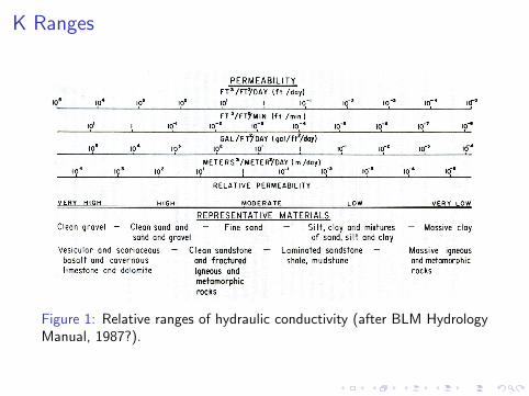
K Ranges
Figure 1: Relative ranges of hydraulic conductivity (after BLM HydrologyManual, 1987?).

T Ranges
Figure 2: Relative ranges of transmissivity and well yield (after BLMHydrology Manual, 1987?). The irrigation-domestic boundary lies at
∼ 0.214m2
sec .

Effect of Scale on Measured K
Figure 3: Effect of tested volume (i.e. heterogeneity) on measured K(Bradbury and Muldoon, 1990).

Flow Equation: Confined Aquifers
I for steady-state system (no change in storage), areal flow(vertical averaging). Flow equation is (see Darcy’s LawNotes):
∂2h
∂x2+
∂2h
∂y2= 0 (1)
I with storage:∂2h
∂x2+
∂2h
∂y2=
S
T· ∂h∂t
(2)

Unconfined Flow
I Dupuit Assumptions: all flow horizontalI hydraulic gradient (∇h) is equal to slope of the water tableI equipotential lines are vertical (no vertical flow, or qz = 0)I Error in this assumption (Bear, 1972):
0 < error <
(∂h∂z
)2
1 +(∂h∂z
)2
I implies smooth free-surface:(∂2h∂x2 ≈ 0
)I this view is inaccurate for “thick” aquifers (Fig. 5)

Unconfined Flow Representative Control Volume
1
2
2
1
∆ x
∆ y
Free Surface
Q
Q
h
h
Figure 4: Mass fluxes for control volume in uniform unconfined flow field.Note free surface (water table) is top surface of volume.

Derivation of Unconfined Flow Equation
I the total discharge or flux Q1 and Q2 can be specified as:
Q1 = q1 ·∆yh1 = −K dhdx
∣∣x1
∆yh1
= −K ∆y
2dh2
dx
∣∣∣x1
Given du2
dx = 2u dudx
Q2 = q2 ·∆yh2 = −K dhdx
∣∣x2
∆yh2
= −K ∆y
2dh2
dx
∣∣∣x2

Derivation of Unconfined Flow Equation (cont.)
I Steady state mass balance (really a volume balance),including recharge onto the free surface:{
rate ofmass in
}−{
rate ofmass out
}= {Source/Sink}
Q1 − Q2 = R∆x∆y
−K∆y
2
dh2
dx
∣∣∣x1
− dh2
dx
∣∣∣x2
∆x
︸ ︷︷ ︸Central difference for d
dx
= R
−K
2d2h2
dx2 = R
K
2d2h2
dx2 = −R

Derivation of Unconfined Flow Equation (cont.)
I Similarly for two dimensions
∂2h2
∂x2+
∂2h2
∂y2= −2R
K

Flow Equation: Unconfined Aquifers
Same development as for confined flow, but now height of controlvolume is h. For a homogeneous unconfined aquifer we obtain theBoussinesq Equation:
∂2h2
∂x2+
∂2h2
∂y2= 0 (3)
with storage:∂2h2
∂x2+
∂2h2
∂y2=
SyT· ∂h∂t
(4)
where Sy is the specific yield, or the amount of water that willgravity drain from a unit volume of aquifer.

Unconfined Flow Approximation
Figure 5: Approximations and true geometry of free surface Freeze and Cherry (after Fig. 5.14, 1979)).Dashed lines are equipotentials, vectors show fluid flow. Top image has a seepage face at E-D, unsaturated flowcrosses the water table. For the middle image K ≡ 0 in the unsaturated zone, the water table is a flowline, bottomfigure shows Dupuit-Forchheimer flow (horizontal only).

Definitions: Rock Property Fields
I Homogeneity: refers to uniform aquifer parameters (i.e.inhomogeneity is the norm in earth materials)
I Isotropy: refers to directional dependence of materialproperties. Usually only hydraulic conductivity is treated asanisotropic (directionally dependent). Anisotropy is describedby giving values along the principal axes of an ellipsoid (e.g.the hydraulic conductivity ellipsoid, Fig. 6)

Hydraulic Conductivity Ellipsoid
sqrt(K )z
sqrt(K )x
x
z
Figure 6: Illustration of the hydraulic conductivity ellipsoid for ananisotropic medium Freeze and Cherry (after Fig. 2.10, 1979)).

Multi-dimensional Darcy’s Law
I need to describe flow in 2- and 3-D situations, must expressDarcy’s Law in multi-dimensional form
I consider ~q as a vector (Fig. 7) the components of the specificdischarge are given by (allowing for anisotropy):
qx = −Kx∂h
∂x
qy = −Ky∂h
∂y(5)
The components are related to one another by
|~q| =√q2x + q2
y
tan θ =qyqx

Vector Velocity
qx
y, j
q
x, i
yq
θ
Figure 7: Vector representation of ~q in two dimensions

3-D Darcy’s Law
I can simply add a Z -component to (5) provided the principalcomponents of the hydraulic conductivity are aligned with thecoordinate axes. In this case (5) can be written in vector form qx
qyqz
= −
Kx
Ky
Kz
· [∂h∂x,∂h
∂y,∂h
∂z
](6)
~q = −K · ∇h (7)
I the most general 3D form of (7) (when principal componentsof conductivity are arbitrarily oriented) expresses conductivityas a second-rank tensor (matrix) (Bear, 1972),
K =
Kxx Kxy Kxz
Kyx Kyy Kyz
Kzx Kzy Kzz
(8)

3-D Darcy’s Law (cont.)
I this tensor is symmetric, i.e. Kxy = Kyx
I the term Kij refers to the i component of conductivity actingin the j direction (e.g. U. Cambridge notes)
I compare to the stress tensor from structural geology

Layered Heterogeneity
I Geologic layering often introduces macroscopic anisotropy(Fig. 8)
I An equivalent homogeneous anisotropic conductivity can bederived (eqns. 3.41-3.42, Fetter, 2001)
I since specific discharge ~q must be constant across each layer,for vertical flow
qz =K1∆h1
d1=
K2∆h2
d2= . . . =
Kz∆h
d
where Kz is the equivalent homogeneous vertical hydraulicconductivity
I rearranging:
Kz =qzd
∆h=
qzdqzd1
K1+ qzd2
K2+ . . .
Kz =d∑n
i=1diKi
(9)

Layered Heterogeneity (cont.)
I similarly the equivalent horizontal conductivity is found bynoting that the total horizontal discharge Qx is just the sum ofthe individual layer discharges:
qh =n∑
i=1
Kidid
∆h
l= Kx
∆h
l
or rearranging
Kx =n∑
i=1
Kidid
(10)

Layered Heterogeneity (cont.)
I e.g. for two layers of 1 m thickness, one with K=10 md , the
other with 100 md , Kh is dominated by the most transmissive
layer, Kz is dominated by least transmissive
Kz =2
110 + 1
100
= =2
0.11
Kh =10
2+
100
2= 110
I the moral here is that complicated problems can often besimplified by combining a bit of geology and math

Effect of Layering on Anisotropy
Figure 8: Anisotropy in hydraulic conductivity caused by layering. Freezeand Cherry (1979, , Fig. 2.9).

Introduction to Flow Nets
I IntroductionI a graphical solution method for potential flow problems (i.e.
solving 2-D Laplace Eqn.)I always handy as an initial solution, can be refined later
through numerical modelingI there are entire books on this methodI Assumptions: homogeneous, saturated, isotropic, steady-state,
no storage (incompressible water & matrix), Darcy’s Law valid
I First Step: Define Boundary ConditionsI constant-head boundaryI no-flow boundary (also constant-flow boundary)I water-table boundary (line of known head at water-table, i.e.
only found in unconfined aquifers, cross-sectional problems)

Construction of Flownets
See Fig. 9
I sketch model area, specify boundary conditions
I draw trial flow lines, extending between constant-headboundaries (i.e. perpendicular to them). Parallel to no-flowboundaries near those boundaries.
I draw trial equipotentials perpendicular to trial flow lines,always perpendicular to them and spaced to form “squares”with the flow lines. Parallel to constant-head boundaries,perpendicular to no-flow boundaries
I adjust repeatedly until an orthogonal set of equipotential andflow lines is generated

Flownet Construction Methodology
Figure 9: General steps in developing a flownet. After (Fig. 4.11, Fetter,2001).

Quantitative Flow Nets
I if care is taken to make areas bounded by equipotentials andstreamlines “square”, discharge through the region of flow canbe calculated
I in most systems, these will be “curvilinear squares”. The bestway to correctly make such a square is to ensure that thesides enclose and are tangent to a circle
I Fetter (eqn 4-55, 2001) gives a formula for this discharge, seealso Freeze and Cherry (eqn. 5.7, 1979).
Q = K∆hm
n(11)
where m is the number of streamtubes (number of streamlinesminus one), and n is the number of head divisions (number ofequipotentials minus one)

Heterogeneity & Flow-Line Refraction
I just as in refraction of light, when water passes from onemedium to another with a different conductivity (i.e. differentvelocity)
I the angle of refraction is Fetter (Fig. 4.13, 2001)
K1
K2=
tanσ1
tanσ2(12)
where σ1 is the angle between the incoming streamline andthe normal to the interface, and σ2 is the angle with theoutgoing streamline (Fig. 10A)
I i.e. for a streamline entering a region of lower conductivity,σ2 < σ1, and the outgoing streamline will bend toward thenormal to the boundary
I this is exactly analogous to Snell’s Law for light rays

Streamline Refraction
Figure 10: Streamline refraction. B) K2 > K1, C) K2 < K1. As inSnell’s Law, the streamline is closer to the normal in the region of lowestvelocity (high index of refraction or low hydraulic conductivity). After(Fig. 4.14, Fetter, 2001).

Flow direction for anisotropic aquifers
I flow direction is not perpendicular to equipotential lines inanisotropic media (i.e. those having Kx 6= Ky , Fig. 6,resulting flownet in Fig. 11)
I flow direction can be estimated graphically when constructingflow nets for anisotropic media (Fig. 12)

Anisotropic Flow Net
Figure 11: Flownet for anisotropic conditions (Ky > Kx). After (Fig.4.10, Fetter, 2001).

Determining Anisotropic Flow Direction
Figure 12: After (Fig. 4.9, Fetter, 2001).

Example Flownets
Figure 13: Flownet for seepage from a channel. a) heterogeneousisotropic KU
KL= 1
50 , b) heterogeneous anisotropic KU
KL= 50, Kx
Kz= 10.
After (Fig. 3.6.3, Todd and Mays, 2005).

Interpreting Potentiometric Surface
Figure 14: Example contour map of potentiometric surface with flowlines. Section 2 has better prospect for a productive well. After (Fig.3.6.5, Todd and Mays, 2005).
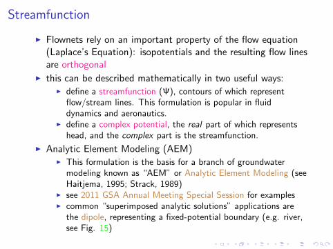
Streamfunction
I Flownets rely on an important property of the flow equation(Laplace’s Equation): isopotentials and the resulting flow linesare orthogonal
I this can be described mathematically in two useful ways:I define a streamfunction (Ψ), contours of which represent
flow/stream lines. This formulation is popular in fluiddynamics and aeronautics.
I define a complex potential, the real part of which representshead, and the complex part is the streamfunction.
I Analytic Element Modeling (AEM)I This formulation is the basis for a branch of groundwater
modeling known as “AEM” or Analytic Element Modeling (seeHaitjema, 1995; Strack, 1989)
I see 2011 GSA Annual Meeting Special Session for examplesI common “superimposed analytic solutions” applications are
the dipole, representing a fixed-potential boundary (e.g. river,see Fig. 15)

Image Wells
Figure 15: Image well method (dipole) (Fig. 2.4, Strack, 1989).

Solving the Flow Equation
Many of the problems in hydrogeology involve solving the flowequation (2) or (4). This will generally involve several of thefollowing approaches:
I analytic solution: exact formula for simple situations (usuallyhomogeneous, isotropic, simplified geometry), generallyderived by direct integration of the flow equation
I graphical solution: usually flownets
I numerical model: required for complex situations, 3-D flow,etc. Currently Modflow is the computer program of choice forgroundwater models

Steady Confined Flow Analytic Solution
I assuming horizontal confined flow in an isotropichomogeneous aquifer (Fig. 16)
I the 2-D flow equation (1) becomes:
d2hdx2 = 0
I seeking a solution for h(x) we integrate the equation twice toobtain the general solution:∫
d2hdx2 dx =
∫0 dx → dh
dx = C1 →∫dhdx dx =
∫C1 dx → h(x) = C1x + C2
I then we use boundary conditions to determine the particularsolution for the case shown in Fig. 16:
I at x = 0, h = h1, which implies C2 = h1

Steady Confined Flow Analytic Solution (cont.)
I at x = L, h = h2. Substituting these values h2 = C1L + h1
and C1 = h2−h1
L
I then the particular solution is:
h =h2 − h1
L· x + h1 (13)
which is the equation for a straight line, as indicated in Fig. 16

Confined Flow Example
Figure 16: Confined flow system example for computation of analyticsolution. Note homogeneity assures that h(x) is a straight line. After(Fig. 4.16, Fetter, 2001).

Steady Unconfined Flow Analytic Solution
I assuming horizontal unconfined flow in an isotropichomogeneous aquifer (Fig. 17)
I the 2-D flow equation (3) becomes:
d2h2
dx2 = 0
I seeking a solution for h(x) we integrate the equation twice toobtain the general solution:∫
d2h2
dx2 dx =
∫0 dx → dh2
dx = C1 →∫dh2
dx dx =
∫C1 dx → h2(x) = C1x + C2
I then we use boundary conditions to determine the particularsolution for the case shown in Fig. 17:
I at x = 0, h = h1, which implies C2 = h21

Steady Unconfined Flow Analytic Solution (cont.)
I at x = L, h = h2. Substituting these values h22 = C1L + h2
1
and C1 =h2
2−h21
L
I then the particular solution is (eqn. 4.71, Fetter, 2001):
h =
√h2
2 − h21
L· x + h2
1 (14)
I allowing for uniform recharge w along the water table, thefinal form is (eqn. 4.70, Fetter, 2001):
h =
√h2
2 − h21
L+ h2
1 +w
K(L− x)x (15)
I several other relationships can be derived from (15), e.g.discharge per unit width q′:
I using Darcy’s Law q′ = −Kh dhdx and noting that du2
dx = 2u dudx
then q′ = −−K2dh2
dx

Steady Unconfined Flow Analytic Solution (cont.)
I differentiating the square of (15)
q′(x) = −−K (
2
[h1 − h2
L+
w
K(L− 2x)
]=
K (h1 − h2)
2L− w
(L
2− x
)

Unconfined Flow Example
Figure 17: Unconfined flow with recharge example for computation ofanalytic solution. Note free surface assures that h(x) is a parabolic line.After (Fig. 4.19, Fetter, 2001).

References
Bear, J.: Dynamics of Fluids in Porous Media. Elsevier, New York, NY(1972)
Bradbury, K.R., Muldoon, M.A.: Hydraulic conductivity determinationsin unlithified glacial and fluvial materials. Special technical pub.,ASTM (1990)
Fetter, C.W.: Applied Hydrogeology. Prentice Hall, Upper Saddle River,NJ, 4th edn. (2001), http://vig.prenhall.com/catalog/academic/product/0,1144,0130882399,00.html
Freeze, R.A., Cherry, J.A.: Groundwater. Prentice-Hall, Englewood Cliffs,NJ (1979)
Haitjema, H.M.: Analytic Element Modeling of Groundwater Flow.Academic Press, San Diego, CA (1995), iSBN 0-12-316550-4
Strack, O.D.L.: Groundwater Mechanics. Prentice Hall, Englewood Cliffs,NJ (1989)
Todd, D.K., Mays, L.W.: Groundwater Hydrology. John Wiley & Sons,Hoboken, NJ, 3rd edn. (2005), http://www.wiley.com/WileyCDA/WileyTitle/productCd-EHEP000351.html


