206-1

Geostatistical Reservoir Characterization of McMurray Formation by 3-D Modeling

Weishan Ren and Clayton V. Deutsch

Department of Civil & Environmental Engineering, University of Alberta

Abstract

Building 3-D models of reservoir properties is always attractive because geological features are inherently three dimensional. 2-D maps fail to capture the complexity of the 3-D variability and connectivity. This paper demonstrates the characterization of the McMurray formation by 3-D modeling of geological facies, porosity, and water saturation over a relatively small area. The “Guide to SAGD Reservoir Characterization Using Geostatistics” prepared by the CCG in April of 2003 was followed to construct the 3-D models illustrated in this paper. We add some implementation details.

Introduction

Reservoir heterogeneity characterization is a big challenge. There is no way to assess the true heterogeneity, but we can create models that mimic the important features of variability. This permits an assessment of uncertainty. We demonstrate the application of geostatistical simulation for the 3-D modeling of reservoir properties.

Geological facies and petrophysical properties, such as porosity, permeability and water saturation, are required in 3-D for uncertainty assessment, delineation planning and production performance prediction. Building a 3-D model over an entire reservoir can be used for input of reservoir flow simulation. A 3-D model in a small area can provide very detailed information on heterogeneity and uncertainty. Such small area models can help to understand the formation better, provide input to the vertical and areal positioning of wells and help calibrate larger scale 2-D models (described in the preceding paper).

We have showed that reservoir characterization of McMurry formation using 2-D modeling (see Paper 205). Although a high resolution 3-D may be built over the entire area of interest, it is often more reasonable to create a number of smaller models. Local variations in the reservoir are best handled with smaller scale models. We demonstrate how to use the 3-D geostatistical modeling to characterize a small area of the McMurray formation. A small synthetic set of data is used for this purpose. The area is 4000m square and the thickness is from the bottom of McMurray formation to the Wabiskaw-McMurray marker. A cell size of 50m by 50m by 0.5m is considered. So, there are 80 by 80 grid cells in the X/Y directions. There are 21 wells in this area. The log data of the 21 wells include depth, facies type, porosity, and water saturation. The resolution of the log data is typically less than 0.5 m; the data must be blocked up to the 0.5m scale. The location map of the wells is shown in Figure 1.

206-2

The structure framework of the 3-D model will be constructed first, then the geological facies model will be built. The porosity model and the water saturation model are built conditional to the facies model.

3-D Structure Framework Modeling

Three structural surfaces are used to define the McMurray in this case. The Wabiskaw-McMurray marker (WMS) is the top surface, the bottom surface of McMurray formation (BSM) is the bottom surface, and a Sequence Boundary Surface (SBS) is used as a middle surface. The Upper Zone (UZ) is from the WMS to SBS, and the Lower Zone (LZ) is from the SBS to BSM. The reason for the two zones is that the reservoir properties in the sand are quite different above and below this surface. The facies and porosity are modeled separately within the two zones. The water saturation, however, uses only the facies and Oil Water Contact (OWC); the stratigraphic surface is not used.

A block centered grid of 50 m by 50 m by 0.5 m is used in the 3D modeling. This gives 80 by 80 or 6400 grid cells in the aerial plain view. There are two types of the vertical coordinate systems used in the 3D modeling. One is the stratigraphic vertical coordinate used for facies modeling and porosity modeling. This coordinate is intended to capture the overall structural correlation within the reservoir, and to account for structural deformation, differential compaction, erosion and onlap geometry. It is assumed that the formation is composed of a sequence of genetically related strata or layers that are parallel to the top surface. So the stratigraphic vertical coordinate can be calculated by the following equation:

strata topZ Z Z= −

where Ztop is the elevation of the top surface, and Z is the real elevation of the data. This vertical coordinate is zero at the top, and higher valued at the bottom. So, when this vertical coordinate is used in plotting, it shows the model upside down in the vertical direction. Based on the data, the boundaries of each formation zone and the number of vertical grids used for the facies and porosity modeling are listed below in Table 1.

Table 1: Boundaries and vertical grids for facies and porosity modeling

Zone Threshold Max-top Min-bottom Thickness Vertical Grid

UZ 26 310 250 60 120 LZ 45 280 180 100 200

The threshold is a vertical elevation used to divide the formation into regions with enough data for vertical trend modeling, see below.

Another coordinate system is the regular vertical coordinate, or the real elevation. Because the water surfaces in formation are nearly flat, the regular vertical coordinate is used for the water saturation modeling. Based on the data, the boundaries of the modeled formation and the number of the vertical grids used for water saturation modeling are listed in Table 2.

206-3

Table 2: Boundaries and vertical grids for water saturation modeling

Zone Up-threshold Low-threshold Min-bottom Max-top Thickness Vertical Grid

UZ 290 -- 270 310 40 80

LZ -- 220 180 270 90 180

3-D Facies Modeling

Generally, petrophysical properties are highly correlated to facies type. The facies are modeled first to constrain the subsequent modeling of porosity and water saturation. The main steps for the cell-based geostatistical facies modeling include (1) gathering and formatting the relevant conditioning data, (2) establishing aerial and vertical trends and combining them into a 3-D proportion/trend model, (3) assembling a licit 3-D variogram model of spatial correlation for each facies type, (4) stochastically constructing the facies realizations.

In the facies modeling, the UZ and the LZ of the McMurray formation are modeled separately. The stratigraphic vertical coordinate is used in the modeling, which is parallel down from top surface.

We consider five facies types for this synthetic example, see table below. Figure 2 shows the histograms of the facies in the area. The sand is dominated in the LZ, and there is no mudstone breccia in the UZ.

Code Facies

1 Sand

2 Mudstone Breccia

3 Sandy Heterolithic Strata (SHS)

4 Muddy Heterolithic Strata (MHS)

5 Mudstone

All conventional geostatistical algorithms have an implicit assumption of stationarity, which assumes the spatial statistics are location independent. Any location-dependent statistics must also be accounted for explicitly. Trends or non-stationary features will be modeled to provide the locally varying mean for the indicator simulation. The vertical facies proportion curves and the 2-D aerial trend of facies proportions are modeled separately. Then, they are combined into 3-D trend model. This data-driven statistical approach is used when the trends are clear; otherwise, no trend is modeled.

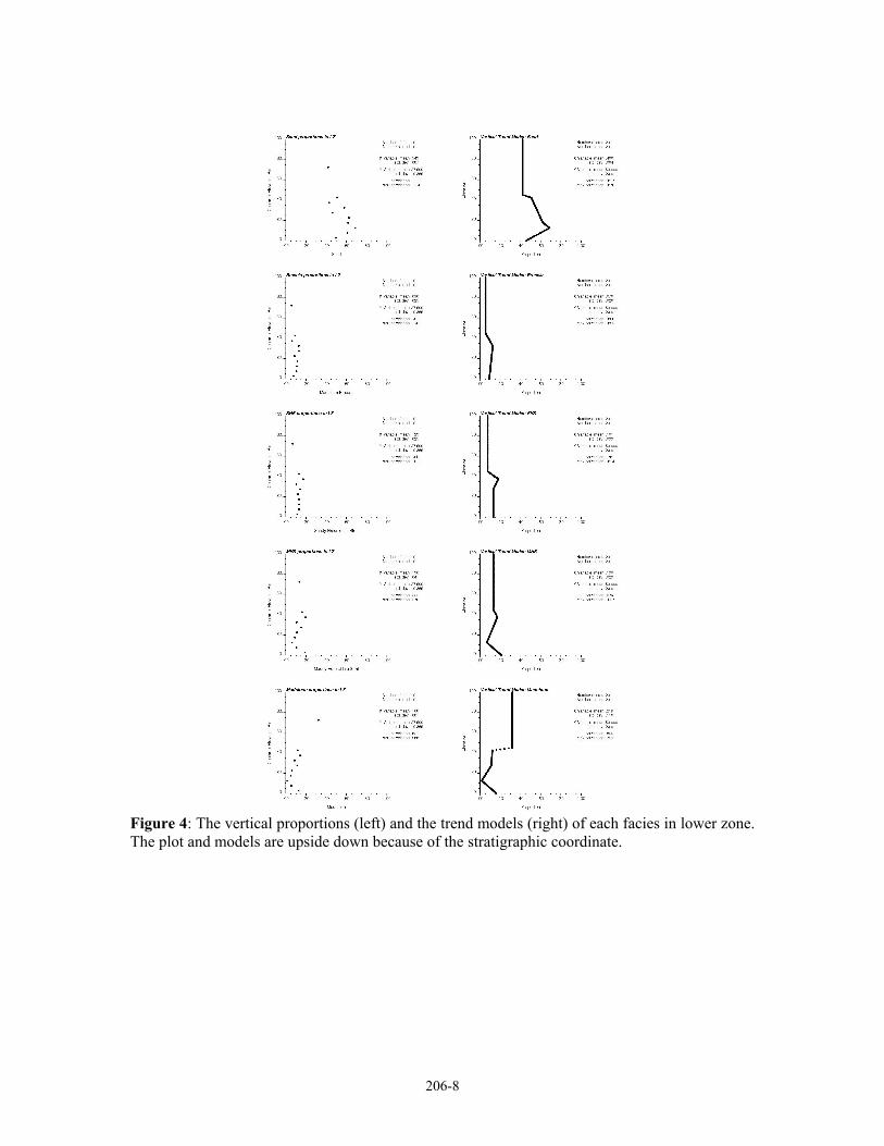
The vertical proportion of each facies is calculated with a bin of 5m in the stratigraphic vertical coordinate. Near the bottom of the formation zones, there are not enough data to calculate a reliable facies proportion. A threshold is selected at the elevation where the number of data is less than half. For the zone below the threshold, all of the data are used to calculate one facies proportion. This proportion will be used as a constant value for the zone from the threshold to the bottom in the vertical trend modeling. The thresholds of each zone are shown as a black line in Figure 3. The plots of calculated facies proportions of the bottom zone are shown on the left side of Figure 4. Because of the vertical coordinate, the model is upside down in the plot. The top is

206-4

at zero. The control points are selected based on the plots, and linear interpolation is used between the control points to inform all elevations. The final 1-D vertical proportion models of bottom zone are shown on right side of Figure 4. Before being used to calculate the 3-D trend model, the five facies models are adjusted to ensure the sum of all proportions at each elevation is one.

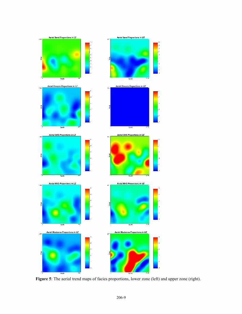
The aerial proportion maps or horizontal trends for lithofacies are created by kriging with the proportion of each facies in each well as conditioning data. The aerial trend maps should reflect the separation of deterministic features and stochastic features in the conditioning data. If they are not clear, it is better to infer less detail than mistakenly incorporate more into the trend model. A synthetic variogram is used to smooth the kriged maps. The aerial trend maps are shown in Figure 5. There are some horizontal trends shown in the top zone, but there is no trend in the bottom zone.

For the case of having both a 1-D vertical proportion trend and a 2-D aerial proportion trend for each facies, a scaling procedure is used to combine them into a 3-D trend model. The approach assumes that the two trends are conditionally independent. The 3-D trend value for each location for each facies can be calculated as the aerial trend multiplied by the vertical trend divided by the global facies proportion at each location for each facies. The scaling procedure takes the following equation:

This scaling procedure is implemented for each facies. The final 3-D proportion trend model will be honored by subsequent sequential indicator simulation, that is, the vertical trend and the form of the aerial trend will be reproduced by lithofacies realizations within the bounds of appropriate stochastic fluctuations.

For the case without 2-D aerial trend, the 3-D trend is generated by simply duplicating the vertical trend at each horizontal grid.

Facies indicator variogram and sequential indicator simulation

The indicator variograms in the horizontal and vertical directions are calculated and modeled to capture the spatial correlation/covariance structure of each facies. The variogram model for sand in lower zone is shown in Figure 6.

Sequential indicator simulation was performed with the 3-D proportion trend model used as locally varying mean. 100 3-D facies realizations were created. After the simulation, the facies realizations are clipped according to the top and bottom structural surfaces; if a particular facies code realization is above the top structure model or below the bottom structure model, it is excluded from the numerical model. Then, the stratigraphic vertical coordinate is converted back to normal coordinate so that the final facies realizations are in real units.

The first facies realization of the bottom zone is shown in Figure 7. This output facies realization has a grid resolution of 50m x 50m aerially and 0.5m vertically. The field spans 4000m, 4000m and 100m in X, Y, and Z directions. This entails 80 x 80 x 200 cells in the Easting (X), Northing (Y) and Elevation (Z) directions, respectively, amounting to 1,280,000 cells in the facies realization. These same grid specifications are used for the 3-D proportion trend models.

_ ( , ) _ ( )( , , )_

areal proportion x y vertical proportion zproportion x y zglobal proportion

×=

206-5

3-D Porosity Modeling

Porosity is strongly controlled by facies. Therefore, the porosity is modeled separately within each facies. The simulation results of porosity are merged using the facies realizations. The main steps of porosity modeling are similar to facies modeling. The top and bottom zones of McMurray formation are also modeled separately. The stratigraphic vertical coordinate is parallel down from top surface.

Trend Modeling

The methodology for creating a 3-D porosity trend within each facies consists of merging a 1-D vertical and 2-D aerial trend into a final 3-D trend model. The result is a 3-D model of locally varying porosity means within sand, mudstone breccia, SHS, MHS, and mudstone facies.

The 1-D vertical porosity trends are calculated by averaging porosity within 5 m vertical bins. The same thresholds as described in the facies modeling are used where there are no enough data. The zones below the thresholds are treated as one bin. The center of each bin is then plotted against the corresponding average porosity values to visualize the general form of the trend. This process is implemented for all five facies types. To infer the trend for the entire vertical range of each formation zone, multiple control points are established on these plots and linear interpolation is implemented.

The 2-D aerial porosity trend maps are created by kriging with the average value of porosity in each well as conditioning data. The same method as used for facies is used to create the 3-D trend models for the cases of with or without 2-D aerial trend, except that the average value is used instead of proportion.

Porosity Variography and Sequential Gaussian Simulation

The porosity will also often exhibit different anisotropy depending on facies. This is accounted for in simulation by creating a separate 3-D variogram model for each lithofacies. The horizontal and vertical variograms of normal-score porosity are calculated and modeled within each facies.

Sequential Gaussian simulation is used to create 100 3-D porosity realizations in each zone and each facies. After all the simulations, a “cookie cutter” approach is used to obtain a merged 3D porosity models. The details should be mentioned. Five complete 3-D models of porosity are simulated; one for each facies, assuming the entire 3-D reservoir is one facies type at a time. These simulations use each of the previously created by-facies porosity data files, trend and variogram models as conditioning data. These five by-facies porosity models are then merged into a new porosity model using the previously created facies models, that is, the new porosity model values are taken from the appropriate facies-dependant model.

After the merging, the porosity realizations are clipped according to the top and bottom structural surfaces. The stratigraphic vertical coordinate is then converted back to present-day vertical coordinates.

The final porosity realization for the bottom zone is shown in Figure 8. This output porosity realization has the same grid specification used for the facies modeling.

206-6

3-D Water Saturation Modeling

Water Saturation (Sw) in the formation also has a correlation to facies. So the water saturation will be modeled on a by-facies basis. Then, the realizations of each facies are merged according to facies realizations.

The McMurray formation is divided into two zones by OWC, which can be determined basing on the vertical trend of water saturation. The regular vertical coordinate is used. The methodology for creating a 3-D water saturation trend within each facies is same as for porosity trend. The only difference is a upper threshold and a lower threshold are used to ensure enough data in each bin.

The horizontal and vertical variograms of normal-score water saturation are calculated and modeled within each facies. Sequential Gaussian simulation is used to create 100 3-D geostatistical realizations of water saturation in each zone and each facies. The realizations are merged into a final water saturation model basing on the facies realizations. After the merging, the water saturation realizations are clipped according to the top and bottom structural surfaces.

The final water saturation realization is shown on the right side of Figure 9. The corresponding facies realizations are plotted beside the Sw realizations.

Comments

100 geological realizations have been constructed for lithofacies, porosity and water saturation. The uncertainty distribution of each property can be generated from each 100 realizations. The 100 realizations can also be used to calculate reservoir parameters, such as net continuous bitumen, bulk oil weight, and to correlate with 2-D models.

Reference

C.V. Deutsch and J.A. McLennan. Guide to SAGD Reservoir Characterization Using Geostatistics. University of Alberta, Edmonton, April 2003.

W. Ren, O. Leuangthong and C.V. Deutsch. Geostatistical Reservoir Characterization of McMurray Formation by 2-D Modeling. University of Alberta, Edmonton, September 2003.

206-7

Figure 1: The location map of wells in the small area

Figure 2: The histograms of facies in lower zone (left) and upper zone (right).

Figure 3: The thresholds are defined in lower zone (left) and upper zone (right).

206-8

Figure 4: The vertical proportions (left) and the trend models (right) of each facies in lower zone. The plot and models are upside down because of the stratigraphic coordinate.

206-9

Figure 5: The aerial trend maps of facies proportions, lower zone (left) and upper zone (right).

206-10

Figure 6: The variogram models of sand in lower zone.

206-11

Figure 7: The first 3-D facies realization of the lower zone. The vertical scale is exaggerated by 40 times.

206-12

Figure 8: The first 3-D porosity realization of the lower zone. The vertical scale is exaggerated by 40 times.

206-13

Figure 9: The first 3-D Facies realization (left) and the first 3-D Sw realization (right). The vertical scale is exaggerated by 40 times.