GERSTEN Solutions Manual to Accompany SMITH An ... · viii CONTENTS 10 An Introduction to Spectral...

Content Type: Black & WhitePaper Type: WhitePage Count: 318File type: Internal

GERSTENSMITH

J A M E S F. E P P E R S O NEPPER

SON

Solutions Manual to Accom

panyAn IN

TRO

DU

CT

ION

to NU

MER

ICA

L MET

HO

DS and A

NA

LYSIS

Second EditionSecondEdition

Solutions Manual to Accompany

An INTRODUCTION to NUMERICAL METHODS and ANALYSIS


AN INTRODUCTION TONUMERICAL METHODSAND ANALYSIS

epperson2 solutions-fm_fitzmmaurice-fm.qxd 7/12/2013 1:30 PM Page i

epperson2 solutions-fm_fitzmmaurice-fm.qxd 7/12/2013 1:30 PM Page ii


AN INTRODUCTION TONUMERICAL METHODSAND ANALYSISSecond Edition

JAMES F. EPPERSON Mathematical Reviews

epperson2 solutions-fm_fitzmmaurice-fm.qxd 7/12/2013 1:30 PM Page iii

Copyright © 2013 by John Wiley & Sons, Inc. All rights reserved.

Published by John Wiley & Sons, Inc., Hoboken, New Jersey.Published simultaneously in Canada.

No part of this publication may be reproduced, stored in a retrieval system or transmitted in any form orby any means, electronic, mechanical, photocopying, recording, scanning or otherwise, except aspermitted under Section 107 or 108 of the 1976 United States Copyright Act, without either the priorwritten permission of the Publisher, or authorization through payment of the appropriate per-copy fee tothe Copyright Clearance Center, Inc., 222 Rosewood Drive, Danvers, MA 01923, (978) 750-8400, fax(978) 750-4470, or on the web at www.copyright.com. Requests to the Publisher for permission shouldbe addressed to the Permissions Department, John Wiley & Sons, Inc., 111 River Street, Hoboken, NJ07030, (201) 748-6011, fax (201) 748-6008, or online at http://www.wiley.com/go/permission.

Limit of Liability/Disclaimer of Warranty: While the publisher and author have used their best efforts inpreparing this book, they make no representation or warranties with respect to the accuracy orcompleteness of the contents of this book and specifically disclaim any implied warranties ofmerchantability or fitness for a particular purpose. No warranty may be created or extended by salesrepresentatives or written sales materials. The advice and strategies contained herein may not be suitablefor your situation. You should consult with a professional where appropriate. Neither the publisher norauthor shall be liable for any loss of profit or any other commercial damages, including but not limitedto special, incidental, consequential, or other damages.

For general information on our other products and services please contact our Customer CareDepartment within the United States at (800) 762-2974, outside the United States at (317) 572-3993 orfax (317) 572-4002.

Wiley also publishes its books in a variety of electronic formats. Some content that appears in print,however, may not be available in electronic formats. For more information about Wiley products, visitour web site at www.wiley.com.

Library of Congress Cataloging-in-Publication Data:

Epperson, James F., author.An introduction to numerical methods and analysis / James F. Epperson, Mathematical Reviews. —

Second edition.pages cm

Includes bibliographical references and index.ISBN 978-1-118-36759-9 (hardback)

1. Numerical analysis. I. Title. QA297.E568 2013518—dc23 2013013979

10 9 8 7 6 5 4 3 2 1

epperson2 solutions-fm_fitzmmaurice-fm.qxd 7/12/2013 1:30 PM Page iv

CONTENTS

1 Introductory Concepts and Calculus Review 1

1.1 Basic Tools of Calculus 11.2 Error, Approximate Equality, and Asymptotic Order Notation 121.3 A Primer on Computer Arithmetic 151.4 A Word on Computer Languages and Software 191.5 Simple Approximations 191.6 Application: Approximating the Natural Logarithm 221.7 A Brief History of Computing 25

2 A Survey of Simple Methods and Tools 27

2.1 Horner’s Rule and Nested Multiplication 272.2 Difference Approximations to the Derivative 302.3 Application: Euler’s Method for Initial Value Problems 402.4 Linear Interpolation 442.5 Application — The Trapezoid Rule 482.6 Solution of Tridiagonal Linear Systems 562.7 Application: Simple Two-Point Boundary Value Problems 61

v

vi CONTENTS

3 Root-Finding 65

3.1 The Bisection Method 653.2 Newton’s Method: Derivation and Examples 693.3 How to Stop Newton’s Method 733.4 Application: Division Using Newton’s Method 773.5 The Newton Error Formula 813.6 Newton’s Method: Theory and Convergence 843.7 Application: Computation of the Square Root 883.8 The Secant Method: Derivation and Examples 923.9 Fixed Point Iteration 963.10 Roots of Polynomials (Part 1) 993.11 Special Topics in Root-finding Methods 1023.12 Very High-order Methods and the Efficiency Index 114

4 Interpolation and Approximation 117

4.1 Lagrange Interpolation 1174.2 Newton Interpolation and Divided Differences 1204.3 Interpolation Error 1324.4 Application: Muller’s Method and Inverse Quadratic

Interpolation 1394.5 Application: More Approximations to the Derivative 1414.6 Hermite Interpolation 1424.7 Piecewise Polynomial Interpolation 1454.8 An Introduction to Splines 1494.9 Application: Solution of Boundary Value Problems 1564.10 Tension Splines 1594.11 Least Squares Concepts in Approximation 1604.12 Advanced Topics in Interpolation Error 166

5 Numerical Integration 171

5.1 A Review of the Definite Integral 1715.2 Improving the Trapezoid Rule 1735.3 Simpson’s Rule and Degree of Precision 1775.4 The Midpoint Rule 1875.5 Application: Stirling’s Formula 1905.6 Gaussian Quadrature 1925.7 Extrapolation Methods 1995.8 Special Topics in Numerical Integration 203

CONTENTS vii

6 Numerical Methods for Ordinary Differential Equations 211

6.1 The Initial Value Problem — Background 2116.2 Euler’s Method 2136.3 Analysis of Euler’s Method 2166.4 Variants of Euler’s Method 2176.5 Single Step Methods — Runge-Kutta 2256.6 Multi-step Methods 2286.7 Stability Issues 2346.8 Application to Systems of Equations 2356.9 Adaptive Solvers 2406.10 Boundary Value Problems 243

7 Numerical Methods for the Solution of Systems of Equations 247

7.1 Linear Algebra Review 2477.2 Linear Systems and Gaussian Elimination 2487.3 Operation Counts 2547.4 The LU Factorization 2567.5 Perturbation, Conditioning and Stability 2627.6 SPD Matrices and the Cholesky Decomposition 2697.7 Iterative Methods for Linear Systems – A Brief Survey 2717.8 Nonlinear Systems: Newton’s Method and Related Ideas 2737.9 Application: Numerical Solution of Nonlinear BVP’s 275

8 Approximate Solution of the Algebraic Eigenvalue Problem 277

8.1 Eigenvalue Review 2778.2 Reduction to Hessenberg Form 2808.3 Power Methods 2818.4 An Overview of the QR Iteration 2848.5 Application: Roots of Polynomials, II 288

9 A Survey of Numerical Methodsfor Partial Differential Equations 289

9.1 Difference Methods for the Diffusion Equation 2899.2 Finite Element Methods for the Diffusion Equation 2939.3 Difference Methods for Poisson Equations 294

viii CONTENTS

10 An Introduction to Spectral Methods 299

10.1 Spectral Methods for Two-Point Boundary Value Problems 29910.2 Spectral Methods for Time-Dependent Problems 30110.3 Clenshaw-Curtis Quadrature 303

Preface to the Solutions Manual

This manual is written for instructors, not students. It includes worked solutions formany (roughly 75%) of the problems in the text. For the computational exercises Ihave given the output generated by my program, or sometimes a program listing. Mostof the programming was done in MATLAB, some in FORTRAN. (The author is wellaware that FORTRAN is archaic, but there is a lot of “legacy code" in FORTRAN,and the author believes there is value in learning a new language, even an archaicone.) When the text has a series of exercises that are obviously similar and havesimilar solutions, then sometimes only one of these problems has a worked solutionincluded. When computational results are asked for a series of similar functions orproblems, only a subset of solutions are reported, largely for the sake of brevity. Someexercises that simply ask the student to perform a straight-forward computation areskipped. Exercises that repeat the same computation but with a different method arealso often skipped, as are exercises that ask the student to “verify” a straight-forwardcomputation.

Some of the exercises were designed to be open-ended and almost “essay-like.”For these exercises, the only solution typically provided is a short hint or brief outlineof the kind of discussion anticipated by the author.

In many exercises the student needs to construct an upper bound on a derivativeof some function in order to determine how small a parameter has to be to achieve a

ix

x

desired level of accuracy. For many of the solutions this was done using a computeralgebra package and the details are not given.

Students who acquire a copy of this manual in order to obtain worked solutions tohomework problems should be aware that none of the solutions are given in enoughdetail to earn full credit from an instructor.

The author freely admits the potential for error in any of these solutions, especiallysince many of the exercises were modified after the final version of the text wassubmitted to the publisher and because the ordering of the exercises was changedfrom the Revised Edition to the Second Edition. While we tried to make all theappropriate corrections, the possibility of error is still present, and undoubtedly theauthor’s responsibility.

Because much of the manual was constructed by doing “copy-and-paste” fromthe files for the text, the enumeration of many tables and figures will be different. Ihave tried to note what the number is in the text, but certainly may have missed someinstances.

Suggestions for new exercises and corrections to these solutions are very welcome.Contact the author at [email protected] or [email protected].

Differences from the text The text itself went through a copy-editing processafter this manual was completed. As was to be expected, the wording of severalproblems was slightly changed. None of these changes should affect the problem interms of what is expected of students; the vast majority of the changes were to replace“previous problem” (a bad habit of mine) with “Problem X.Y” (which I should havedone on my own, in the first place). Some puncuation was also changed. The point ofadding this note is to explain the textual differences which might be noticed betweenthe text and this manual. If something needs clarification, please contact me at theabove email.

CHAPTER 1

INTRODUCTORY CONCEPTS ANDCALCULUS REVIEW

1.1 BASIC TOOLS OF CALCULUS

Exercises:

1. Show that the third order Taylor polynomial for f(x) = (x + 1)−1, aboutx0 = 0, is

p3(x) = 1− x+ x2 − x3.

Solution: We have f(0) = 1 and

f ′(x) = − 1

(x+ 1)2, f ′′(x) =

2

(x+ 1)3, f ′′′(x) = − 6

(x+ 1)4,

so that f ′(0) = −1, f ′′(0) = 2, f ′′′ = −6. Therefore

p3(x) = f(0) + xf ′(0) +1

2x2f ′′(0) +

1

6x3f ′′′(x)

= 1 + x(−1) +1

2x2(2) +

1

6x3(−6)

= 1− x+ x2 − x3.

Solutions Manual to Accompany An Introduction to Numerical Methods and Analysis,Second Edition. By James F. EppersonCopyright c© 2013 John Wiley & Sons, Inc.

1

2 INTRODUCTORY CONCEPTS AND CALCULUS REVIEW

2. What is the third order Taylor polynomial for f(x) =√x+ 1, about x0 = 0?

Solution: We have f(x0) = 1 and

f ′(x) =1

2(x+ 1)1/2, f ′′(x) = − 1

4(x+ 1)3/2, f ′′′(x) =

3

8(x+ 1)5/2,

so that f ′(0) = 1/2, f ′′(0) = −1/4, f ′′′ = 3/8. Therefore

p3(x) = f(0) + xf ′(0) +1

2x2f ′′(0) +

1

6x3f ′′′(x)

= 1 + x(1/2) +1

2x2(−1/4) +

1

6x3(3/8)

= 1− (1/2)x− (1/8)x2 + (1/16)x3.

3. What is the sixth order Taylor polynomial for f(x) =√

1 + x2, using x0 = 0?Hint: Consider the previous problem.

4. Given that

R(x) =|x|6

6!eξ

for x ∈ [−1, 1], where ξ is between x and 0, find an upper bound for |R|, validfor all x ∈ [−1, 1], that is independent of x and ξ.

5. Repeat the above, but this time require that the upper bound be valid only forall x ∈ [− 1

2 ,12 ].

Solution: The only significant difference is the introduction of a factor of 26

in the denominator:

|R(x)| ≤√e

26 × 720= 3.6× 10−5.

6. Given that

R(x) =|x|4

4!

(−1

1 + ξ

)for x ∈ [− 1

2 ,12 ], where ξ is between x and 0, find an upper bound for |R|, valid

for all x ∈ [− 12 ,

12 ], that is independent of x and ξ.

7. Use a Taylor polynomial to find an approximate value for√e that is accurate

to within 10−3.

Solution: There’s two ways to do this. We can approximate f(x) = ex anduse x = 1/2, or we can approximate g(x) =

√x and use x = e. In addition,

we can be conventional and take x0 = 0, or we can take x0 6= 0 in order tospeed convergence.

BASIC TOOLS OF CALCULUS 3

The most straightforward approach (in my opinion) is to use a Taylor polyno-mial for ex about x0 = 0. The remainder after k terms is

Rk(x) =xk+1

(k + 1)!eξ.

We quickly have that

|Rk(x)| ≤ e1/2

2k+1(k + 1)!

and a little playing with a calculator shows that

|R3(x)| ≤ e1/2

16× 24= 0.0043

but

|R4(x)| ≤ e1/2

32× 120= 4.3× 10−4.

So we would use

e1/2 ≈ 1 +1

2+

1

2

(1

2

)2

+1

6

(1

2

)3

+1

24

(1

2

)4

= 1.6484375.

To fourteen digits,√e = 1.64872127070013, and the error is 2.84 × 10−4,

much smaller than required.

8. What is the fourth order Taylor polynomial for f(x) = 1/(x + 1), aboutx0 = 0?

Solution: We have f(0) = 1 and

f ′(x) = − 1

(x+ 1)2, f ′′(x) =

2

(x+ 1)3, f ′′′(x) = − 6

(x+ 1)4, f ′′′′(x) =

24

(x+ 1)5

so that f ′(0) = −1, f ′′(0) = 2, f ′′′ = −6, f ′′′′(0) = 24. Thus

p4(x) = 1+x(−1)+1

2x2(2)+

1

6x3(−6)+

1

24x4(24) = 1−x+x2−x3+x4.

9. What is the fourth order Taylor polynomial for f(x) = 1/x, about x0 = 1?

10. Find the Taylor polynomial of third order for sinx, using:

(a) x0 = π/6.

Solution: We have

f(x0) =1

2, f ′(x0) =

√3

2, f ′′(x0) = −1

2, f ′′′(x0) = −

√3

2,


so

p3(x) =1

2+

√3

2

(x− π

6

)− 1

4

(x− π

6

)2−√

3

12

(x− π

6

)3.

(b) x0 = π/4;

(c) x0 = π/2;

11. For each function below construct the third-order Taylor polynomial approx-imation, using x0 = 0, and then estimate the error by computing an upperbound on the remainder, over the given interval.

(a) f(x) = e−x, x ∈ [0, 1];

(b) f(x) = ln(1 + x), x ∈ [−1, 1];

(c) f(x) = sinx, x ∈ [0, π];

(d) f(x) = ln(1 + x), x ∈ [−1/2, 1/2];

(e) f(x) = 1/(x+ 1), x ∈ [−1/2, 1/2].

Solution:

(a) The polynomial is

p3(x) = 1− x+1

2x2 − 1

6x3,

with remainderR3(x) =

1

24x4e−ξ.

This can be bounded above, for all x ∈ [0, 1], by

|R3(x)| ≤ 1

24e

(b) The polynomial is

p3(x) = x− 1

2x2 +

1

3x3,

with remainderR3(x) =

1

4x4

1

(1 + ξ)4

We can’t bound this for all x ∈ [−1, 1], because of the potential divisionby zero.

(c) The polynomial is

p3(x) = x− 1

6x3


with remainder

R3(x) =1

120x5 cos ξ.

This can be bounded above, for all x ∈ [0, π], by

|R3(x)| ≤ π5

120.

(d) The polynomial is the same as in (b), of course,

p3(x) = x− 1

2x2 +

1

3x3,

with remainder

R3(x) =1

4x4

1

(1 + ξ)4

For all x ∈ [−1/2, 1/2] this can be bounded by

R3(x) ≤ 1

4(1/24)

1

(1− (1/2))4=

1

4.

(e) The polynomial is

p3(x) = 1− x+ x2 − x3,

with remainder

R3(x) = x41

(1 + ξ)5

This can be bounded above, for all x ∈ [−1/2, 1/2], by

|R3(x)| ≤ (1/2)41

(1− 1/2)5= 2.

Obviously, this is not an especialy good approximation.

12. Construct a Taylor polynomial approximation that is accurate to within 10−3,over the indicated interval, for each of the following functions, using x0 = 0.

(a) f(x) = sinx, x ∈ [0, π];

(b) f(x) = e−x, x ∈ [0, 1];

(c) f(x) = ln(1 + x), x ∈ [−1/2, 1/2];

(d) f(x) = 1/(x+ 1), x ∈ [−1/2, 1/2];

(e) f(x) = ln(1 + x), x ∈ [−1, 1].


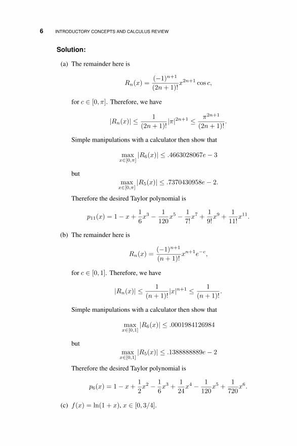
Solution:

(a) The remainder here is

Rn(x) =(−1)n+1

(2n+ 1)!x2n+1 cos c,

for c ∈ [0, π]. Therefore, we have

|Rn(x)| ≤ 1

(2n+ 1)!|π|2n+1 ≤ π2n+1

(2n+ 1)!.

Simple manipulations with a calculator then show that

maxx∈[0,π]

|R6(x)| ≤ .4663028067e− 3

butmaxx∈[0,π]

|R5(x)| ≤ .7370430958e− 2.

Therefore the desired Taylor polynomial is

p11(x) = 1− x+1

6x3 − 1

120x5 − 1

7!x7 +

1

9!x9 +

1

11!x11.

(b) The remainder here is

Rn(x) =(−1)n+1

(n+ 1)!xn+1e−c,

for c ∈ [0, 1]. Therefore, we have

|Rn(x)| ≤ 1

(n+ 1)!|x|n+1 ≤ 1

(n+ 1)!.

Simple manipulations with a calculator then show that

maxx∈[0,1]

|R6(x)| ≤ .0001984126984

butmaxx∈[0,1]

|R5(x)| ≤ .1388888889e− 2

Therefore the desired Taylor polynomial is

p6(x) = 1− x+1

2x2 − 1

6x3 +

1

24x4 − 1

120x5 +

1

720x6.

(c) f(x) = ln(1 + x), x ∈ [0, 3/4].


Solution: The remainder is now

|Rn(x)| ≤ (1/2)n+1

(n+ 1),

and n = 8 makes the error small enough.(d) f(x) = ln(1 + x), x ∈ [0, 1/2].

13. Repeat the above, this time with a desired accuracy of 10−6.

14. Sinceπ

4= arctan 1,

we can estimate π by estimating arctan 1. How many terms are needed inthe Gregory series for the arctangent to approximate π to 100 decimal places?1,000? Hint: Use the error term in the Gregory series to predict when the errorgets sufficiently small.

Solution: The remainder in the Gregory series approximation is

Rn(x) = (−1)n+1

∫ x

0

t2n+2

1 + t2dt,

so to get 100 decimal places of accuracy for x = 1, we require

|Rn(1)| =∣∣∣∣∫ 1

0

t2n+2

1 + t2dt

∣∣∣∣ ≤ ∫ 1

0

t2n+2dt =1

2n+ 3≤ 10−100,

thus, we have to take n ≥ (10100 − 3)/2 terms. For 1,000 places of accuracywe therefore need n ≥ (101000 − 3)/2 terms.

Obviously this is not the best procedure for computing many digits of π!

15. Elementary trigonometry can be used to show that

arctan(1/239) = 4 arctan(1/5)− arctan(1).

This formula was developed in 1706 by the English astronomer John Machin.Use this to develop a more efficient algorithm for computing π. How manyterms are needed to get 100 digits of accuracy with this form? How manyterms are needed to get 1,000 digits? Historical note: Until 1961 this was thebasis for the most commonly used method for computing π to high accuracy.

Solution: We now have two Gregory series, thus complicating the problem abit. We have

π = 4 arctan(1) = 16 arctan(1/5)− 4 arctan(1/239);

Define pm,n ≈ π as the approximation generated by using an m term Gre-gory series to approximate arctan(1/5) and an n term Gregory series forarctan(1/239). Then we have

pm,n − π = 16Rm(1/5)− 4Rn(1/239),


where Rk is the remainder in the Gregory series. Therefore

|pm,n − π| ≤

∣∣∣∣∣16(−1)m+1

∫ 1/5

0

t2m+2

1 + t2dt− 4(−1)n+1

∫ 1/239

0

t2n+2

1 + t2dt

∣∣∣∣∣≤ 16

(2m+ 3)52m+3+

4

(2n+ 3)2392n+3.

To finish the problem we have to apportion the error between the two series,which introduces some arbitrariness into the the problem. If we require thatthey be equally accurate, then we have that

16

(2m+ 3)52m+3≤ ε

and4

(2n+ 3)2392n+3≤ ε.

Using properties of logarithms, these become

log(2m+ 3) + (2m+ 3) log 5 ≥ log 16− log ε

andlog(2n+ 3) + (2n+ 3) log 239 ≥ log 4− log ε.

For ε = (1/2) × 10−100 these are satisfied for m = 70, n = 20. Forε = (1/2)× 10−1000 we get m = 712, n = 209. Changing the apportionmentof the error doesn’t change the results by much at all.

16. In 1896 a variation on Machin’s formula was found:

arctan(1/239) = arctan(1)− 6 arctan(1/8)− 2 arctan(1/57),

and this began to be used in 1961 to compute π to high accuracy. How manyterms are needed when using this expansion to get 100 digits of π? 1,000digits?

Solution: We now have three series to work with, which complicates mattersonly slightly more compared to the previous problem. If we define pk,m,n ≈ πbased on

π = 4 arctan(1) = 24 arctan(1/8) + 8 arctan(1/57) + 4 arctan(1/239),

taking k terms in the series for arctan(1/8), m terms in the series forarctan(1/57), and n terms in the series for arctan(1/239), then we are led tothe inequalities

log(2k + 3) + (2k + 3) log 8 ≥ log 24− log ε,

log(2m+ 3) + (2m+ 3) log 57 ≥ log 8− log ε,


andlog(2n+ 3) + (2n+ 3) log 239 ≥ log 4− log ε.

For ε = (1/3) × 10−100 we get k = 54, m = 27, and n = 19; for ε =(1/3)× 10−1000 we get k = 552, m = 283, and n = 209.

Note: In both of these problems a slightly more involved treatment of the errormight lead to fewer terms being required.

17. What is the Taylor polynomial of order 3 for f(x) = x4 + 1, using x0 = 0?

Solution: This is very direct:

f ′(x) = 4x3, f ′′(x) = 12x2, f ′′′(x) = 24x,

so that

p3(x) = 1 + x(0) +1

2x2(0) +

1

6x3(0) = 1.

18. What is the Taylor polynomial of order 4 for f(x) = x4 + 1, using x0 = 0?Simplify as much as possible.

19. What is the Taylor polynomial of order 2 for f(x) = x3 + x, using x0 = 1?

20. What is the Taylor polynomial of order 3 for f(x) = x3 + x, using x0 = 1?Simplify as much as possible.

Solution: We note that f ′′′(1) = 6, so we have (using the solution from theprevious problem)

p4(x) = 3x2 − 2x+ 1 +1

6(x− 1)3(6) = x3 + x.

The polynomial is its own Taylor polynomial.

21. Let p(x) be an arbitrary polynomial of degree less than or equal to n. What isits Taylor polynomial of degree n, about an arbitrary x0?

22. The Fresnel integrals are defined as

C(x) =

∫ x

0

cos(πt2/2)dt

and

S(x) =

∫ x

0

sin(πt2/2)dt.

Use Taylor expansions to find approximations to C(x) and S(x) that are 10−4

accurate for all x with |x| ≤ 12 . Hint: Substitute x = πt2/2 into the Taylor

expansions for the cosine and sine.


Solution: We will show the work for the case of S(x), only. We have

S(x) =

∫ x

0

sin(πt2/2)dt =

∫ x

0

pn(t2)dt+

∫ x

0

Rn(t2)dt.

Looking more carefully at the remainder term, we see that it is given by

rn(x) = ±∫ x

0

(t2(2n+3)

(2n+ 3)!cos ξdt.

Therefore,

|rn(x)| ≤∫ 1/2

0

(t2(2n+3)

(2n+ 3)!dt =

(1/2)4n+7

(4n+ 7)(2n+ 3)!.

A little effort with a calculator shows that this is less than 10−4 for n ≥ 1,therefore the polynomial is

p(x) =

∫ x

0

(t2 − (1/6)t6)dt = −x7

42+x3

3.

23. Use the Integral Mean Value Theorem to show that the “pointwise” form (1.3)of the Taylor remainder (usually called the Lagrange form) follows from the“integral” form (1.2) (usually called the Cauchy form).

24. For each function in Problem 11, use the Mean Value Theorem to find a valueM such that

|f(x1)− f(x2)| ≤M |x1 − x2|

is valid for all x1, x2 in the interval used in Problem 11.

Solution: This amounts to finding an upper bound on |f ′| over the intervalgiven. The answers are as given below.

(a) f(x) = e−x, x ∈ [0, 1]; M ≤ 1.

(b) f(x) = ln(1+x), x ∈ [−1, 1];M is unbounded, since f ′(x) = 1/(1+x)and x = −1 is possible.

(c) f(x) = sinx, x ∈ [0, π]; M ≤ 1.

(d) f(x) = ln(1 + x), x ∈ [−1/2, 1/2]; M ≤ 2.

(e) f(x) = 1/(x+ 1), x ∈ [−1/2, 1/2]. M ≤ 4.

25. A function is called monotone on an interval if its derivative is strictly positiveor strictly negative on the interval. Suppose f is continuous and monotoneon the interval [a, b], and f(a)f(b) < 0; prove that there is exactly one valueα ∈ [a, b] such that f(α) = 0.

Solution: Since f is continuous on the interval [a, b] and f(a)f(b) < 0, theIntermediate Value Theorem guarantees that there is a point c where f(c) = 0,


i.e., there is at least one root. Suppose now that there exists a second root, γ.Then f(c) = f(γ) = 0. By the Mean Value Theorem, then, there is a point ξbetween c and γ such that

f ′(ξ) =f(γ)− f(c)

γ − c= 0.

But this violates the hypothesis that f is monotone, since a monotone functionmust have a derivative that is strictly positive or strictly negative. Thus wehave a contradiction, thus there cannot exist the second root.

A very acceptable argument can be made by appealing to a graph of thefunction.

26. Finish the proof of the Integral Mean Value Theorem (Theorem 1.5) by writingup the argument in the case that g is negative.

Solution: All that is required is to observe that if g is negative, then we have∫ b

a

g(t)f(t)dt ≤∫ b

a

g(t)fmdt = fm

∫ b

a

g(t)dt

and ∫ b

a

g(t)f(t)dt ≥∫ b

a

g(t)fMdt = fM

∫ b

a

g(t)dt.

The proof is completed as in the text.

27. Prove Theorem 1.6, providing all details.

28. Let ck > 0, be given, 1 ≤ k ≤ n, and let xk ∈ [a, b], 1 ≤ k ≤ n. Then, use theDiscrete Average Value Theorem to prove that, for any function f ∈ C([a, b]),∑n

k=1 ckf(xk)∑nk=1 ck

= f(ξ)

for some ξ ∈ [a, b].

Solution: We can’t apply the Discrete Average Value Theorem to the problemas it is posed originally, so we have to manipulate a bit. Define

γj =cj∑nk=1 ck

;

Thenn∑j=1

γj = 1

and now we can apply the Discrete Average Value Theorem to finish theproblem.


29. Discuss, in your own words, whether or not the following statement is true:“The Taylor polynomial of degree n is the best polynomial approximation ofdegree n to the given function near the point x0.”

/ • • • .

1.2 ERROR, APPROXIMATE EQUALITY, AND ASYMPTOTIC ORDERNOTATION

Exercises:

1. Use Taylor’s Theorem to show that ex = 1 + x + O(x2) for x sufficientlysmall.

2. Use Taylor’s Theorem to show that 1−cos xx = 1

2x + O(x3) for x sufficientlysmall.

Solution: We can expand the cosine in a Taylor series as

cosx = 1− 1

2x2 +

1

24x4 cos ξ.

If we substitute this into (1− cosx)/x and simplify, we get

1− cosx

x=

1

2x− 1

24x3 cos ξ,

so that we have∣∣∣∣1− cosx

x− 1

2x

∣∣∣∣ =

∣∣∣∣ 1

24x3 cos ξ

∣∣∣∣ ≤ 1

24|x3| = C|x3|

where C = 1/24. Therefore, 1−cos xx = 1

2x+O(x3).

3. Use Taylor’s Theorem to show that

√1 + x = 1 +

1

2x+O(x2)

for x sufficiently small.

Solution: We have, from Taylor’s Theorem, with x0 = 0,

√1 + x = 1 +

1

2x− 1

8x2(1 + ξ)−3/2,

for some ξ between 0 and x. Since∣∣∣∣18x2(1 + ξ)−3/2∣∣∣∣ ≤ C|x2|

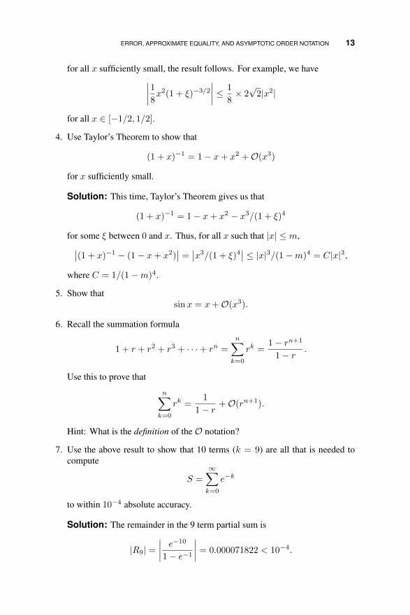
ERROR, APPROXIMATE EQUALITY, AND ASYMPTOTIC ORDER NOTATION 13

for all x sufficiently small, the result follows. For example, we have∣∣∣∣18x2(1 + ξ)−3/2∣∣∣∣ ≤ 1

8× 2√

2|x2|

for all x ∈ [−1/2, 1/2].

4. Use Taylor’s Theorem to show that

(1 + x)−1 = 1− x+ x2 +O(x3)

for x sufficiently small.

Solution: This time, Taylor’s Theorem gives us that

(1 + x)−1 = 1− x+ x2 − x3/(1 + ξ)4

for some ξ between 0 and x. Thus, for all x such that |x| ≤ m,∣∣(1 + x)−1 − (1− x+ x2)∣∣ =

∣∣x3/(1 + ξ)4∣∣ ≤ |x|3/(1−m)4 = C|x|3,

where C = 1/(1−m)4.

5. Show thatsinx = x+O(x3).

6. Recall the summation formula

1 + r + r2 + r3 + · · ·+ rn =n∑k=0

rk =1− rn+1

1− r.

Use this to prove that

n∑k=0

rk =1

1− r+O(rn+1).

Hint: What is the definition of the O notation?

7. Use the above result to show that 10 terms (k = 9) are all that is needed tocompute

S =

∞∑k=0

e−k

to within 10−4 absolute accuracy.

Solution: The remainder in the 9 term partial sum is

|R9| =∣∣∣∣ e−10

1− e−1

∣∣∣∣ = 0.000071822 < 10−4.


8. Recall the summation formula

n∑k=1

k =n(n+ 1)

2.

Use this to show thatn∑k=1

k =1

2n2 +O(n).

9. State and prove the version of Theorem 1.7 which deals with relationships ofthe form x = xn +O(β(n)).

Solution: The theorem statement might be something like the following:

Theorem: Let x = xn+O(β(n)) and y = yn+O(γ(n)), with bβ(n) > γ(n)for all n sufficiently large. Then

x+ y = xn + yn +O(β(n) + γ(n)),

x+ y = xn + yn +O(β(n)),

Ax = Axn +O(β(n)).

In the last equation, A is an arbitrary constant, independent of n.

The proof parallels the one in the text almost perfectly, and so is omitted.

10. Use the definition of O to show that if y = yh + O(hp), then hy = hyh +O(hp+1).

11. Show that if an = O(np) and bn = O(nq), then anbn = O(np+q).

Solution: We have|an| ≤ Ca|np|

and|bn| ≤ Cb|nq|.

These follow from the definition of the O notation. Therefore

|anbn| ≤ Ca|np||bn| ≤ (Ca|np|)(Cb|nq|) = (CaCb)|np+q|

which implies that anbn = O(np+q).

12. Suppose that y = yh + O(β(h)) and z = zh + O(β(h)), for h sufficientlysmall. Does it follow that y − z = yh − zh (for h sufficiently small)?

13. Show that

f ′′(x) =f(x+ h)− 2f(x) + f(x− h)

h2+O(h2)

A PRIMER ON COMPUTER ARITHMETIC 15

for all h sufficiently small. Hint: Expand f(x ± h) out to the fourth orderterms.

Solution: This is a straight-forward manipulation with the Taylor expansions

f(x+ h) = f(x) + hf ′(x) +1

2h2f ′′(x) +

1

6h3f ′′′(x) +

1

24h4f ′′′′(ξ1)

and

f(x− h) = f(x)− hf ′(x) +1

2h2f ′′(x)− 1

6h3f ′′′(x) +

1

24h4f ′′′′(ξ2).

Add the two expansions to get

f(x+ h) + f(x− h) = 2f(x) + h2f ′′(x) +1

24h4(f ′′′′(ξ1) + f ′′′′(ξ2)).

Now solve for f ′′(x).

14. Explain, in your own words, why it is necessary that the constant C in (1.8) beindependent of h.

/ • • • .

1.3 A PRIMER ON COMPUTER ARITHMETIC

Exercises:

1. In each problem below, A is the exact value, and Ah is an approximation to A.Find the absolute error and the relative error.

(a) A = π, Ah = 22/7;

(b) A = e, Ah = 2.71828;

(c) A = 16 , Ah = 0.1667;

(d) A = 16 , Ah = 0.1666.

Solution:

(a) Abs. error. ≤ 1.265× 10−3, rel. error ≤ 4.025× 10−4;

(b) Abs. error. ≤ 1.828× 10−6, rel. error ≤ 6.72× 10−7;

(c) Abs. error. ≤ 3.334× 10−5, rel. error ≤ 2.000× 10−4;

(d) Abs. error. ≤ 6.667× 10−5, rel. error ≤ 4× 10−4.

2. Perform the indicated computations in each of three ways: (i) Exactly; (ii)Using three-digit decimal arithmetic, with chopping; (iii) Using three-digit


decimal arithmetic, with rounding. For both approximations, compute theabsolute error and the relative error.

(a) 16 + 1

10 ;(b) 1

6 ×110 ;

(c) 19 +

(17 + 1

6

);

(d)(17 + 1

6

)+ 1

9 .

3. For each function below explain why a naive construction will be susceptibleto significant rounding error (for x near certain values), and explain how toavoid this error.

(a) f(x) = (√x+ 9− 3)x−1;

(b) f(x) = x−1(1− cosx);(c) f(x) = (1− x)−1(lnx− sinπx);(d) f(x) = (cos(π + x)− cosπ)x−1;(e) f(x) = (e1+x − e1−x)(2x)−1;

Solution: In each case, the function is susceptible to subtractive cancellationwhich will be amplified by division by a small number. The way to avoid theproblem is to use a Taylor expansion to make the subtraction and division bothexplicit operations. For instance, in (a), we would write

f(x) = ((3+(1/6)x−(1/216)x2+O(x3))−3)x−1 = (1/6)−(1/216)x+O(x2).

To get greater accuracy, take more terms in the Taylor expansion.

4. For f(x) = (ex − 1)/x, how many terms in a Taylor expansion are needed toget single precision accuracy (7 decimal digits) for all x ∈ [0, 12 ]? How manyterms are needed for double precision accuracy (14 decimal digits) over thissame range?

5. Using single precision arithmetic, only, carry out each of the following com-putations, using first the form on the left side of the equals sign, then using theform on the right side, and compare the two results. Comment on what youget in light of the material in 1.3.

(a) (x+ ε)3 − 1 = x3 + 3x2ε+ 3xε2 + ε3 − 1, x = 1.0, ε = 0.000001.(b) −b+

√b2 − 2c = 2c(−b−

√b2 − 2c)−1, b = 1, 000, c = π.

Solution: “Single precision” means 6 or 7 decimal digits, so the point of theproblem is to do the computations using 6 or 7 digits.

(a) Using a standard FORTRAN compiler on a low-end UNIX workstation,the author got

(x+ ε)3 − 1 = 0.2861022949218750E − 05

A PRIMER ON COMPUTER ARITHMETIC 17

but

x3 + 3x2ε+ 3xε2 + ε3 − 1 = 0.2980232238769531E − 05.

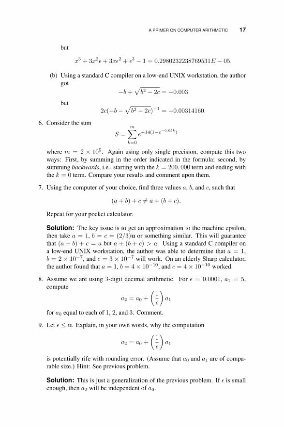
(b) Using a standard C compiler on a low-end UNIX workstation, the authorgot

−b+√b2 − 2c = −0.003

but2c(−b−

√b2 − 2c)−1 = −0.00314160.

6. Consider the sum

S =m∑k=0

e−14(1−e−0.05k)

where m = 2 × 105. Again using only single precision, compute this twoways: First, by summing in the order indicated in the formula; second, bysumming backwards, i.e., starting with the k = 200, 000 term and ending withthe k = 0 term. Compare your results and comment upon them.

7. Using the computer of your choice, find three values a, b, and c, such that

(a+ b) + c 6= a+ (b+ c).

Repeat for your pocket calculator.

Solution: The key issue is to get an approximation to the machine epsilon,then take a = 1, b = c = (2/3)u or something similar. This will guaranteethat (a + b) + c = a but a + (b + c) > a. Using a standard C compiler ona low-end UNIX workstation, the author was able to determine that a = 1,b = 2 × 10−7, and c = 3 × 10−7 will work. On an elderly Sharp calculator,the author found that a = 1, b = 4× 10−10, and c = 4× 10−10 worked.

8. Assume we are using 3-digit decimal arithmetic. For ε = 0.0001, a1 = 5,compute

a2 = a0 +

(1

ε

)a1

for a0 equal to each of 1, 2, and 3. Comment.

9. Let ε ≤ u. Explain, in your own words, why the computation

a2 = a0 +

(1

ε

)a1

is potentially rife with rounding error. (Assume that a0 and a1 are of compa-rable size.) Hint: See previous problem.

Solution: This is just a generalization of the previous problem. If ε is smallenough, then a2 will be independent of a0.


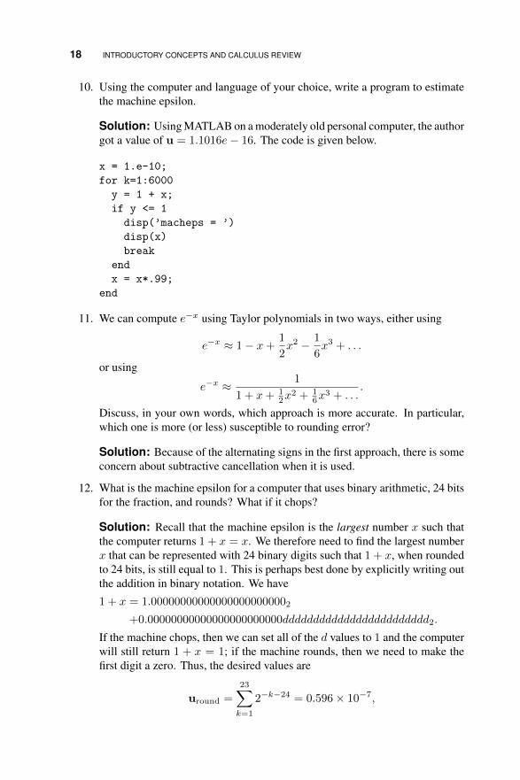
10. Using the computer and language of your choice, write a program to estimatethe machine epsilon.

Solution: Using MATLAB on a moderately old personal computer, the authorgot a value of u = 1.1016e− 16. The code is given below.

x = 1.e-10;

for k=1:6000

y = 1 + x;

if y <= 1

disp(’macheps = ’)

disp(x)

break

end

x = x*.99;

end

11. We can compute e−x using Taylor polynomials in two ways, either using

e−x ≈ 1− x+1

2x2 − 1

6x3 + . . .

or using

e−x ≈ 1

1 + x+ 12x

2 + 16x

3 + . . ..

Discuss, in your own words, which approach is more accurate. In particular,which one is more (or less) susceptible to rounding error?

Solution: Because of the alternating signs in the first approach, there is someconcern about subtractive cancellation when it is used.

12. What is the machine epsilon for a computer that uses binary arithmetic, 24 bitsfor the fraction, and rounds? What if it chops?

Solution: Recall that the machine epsilon is the largest number x such thatthe computer returns 1 + x = x. We therefore need to find the largest numberx that can be represented with 24 binary digits such that 1 + x, when roundedto 24 bits, is still equal to 1. This is perhaps best done by explicitly writing outthe addition in binary notation. We have

1 + x = 1.000000000000000000000002

+0.00000000000000000000000dddddddddddddddddddddddd2.

If the machine chops, then we can set all of the d values to 1 and the computerwill still return 1 + x = 1; if the machine rounds, then we need to make thefirst digit a zero. Thus, the desired values are

uround =23∑k=1

2−k−24 = 0.596× 10−7,

Date post:	19-Mar-2020
Category:	Documents
Upload:	others
View:	2 times
Download:	0 times

GERSTEN Solutions Manual to Accompany SMITH An ... · viii CONTENTS 10 An Introduction to Spectral...

Documents