Pairs trading

Gesina Gorter

December 12, 2006

Contents

1 Introduction 31.1 IMC . . . . . . . . . . . . . . . . . . . . . . . . . . . . . . . . 31.2 Pairs trading . . . . . . . . . . . . . . . . . . . . . . . . . . . 41.3 Graduation project . . . . . . . . . . . . . . . . . . . . . . . . 51.4 Outline . . . . . . . . . . . . . . . . . . . . . . . . . . . . . . . 6

2 Trading strategy 72.1 Introductory example . . . . . . . . . . . . . . . . . . . . . . . 82.2 Data . . . . . . . . . . . . . . . . . . . . . . . . . . . . . . . . 142.3 Properties of pairs trading . . . . . . . . . . . . . . . . . . . . 152.4 Trading strategy . . . . . . . . . . . . . . . . . . . . . . . . . 172.5 Conclusion . . . . . . . . . . . . . . . . . . . . . . . . . . . . . 26

3 Time series basics 27

4 Cointegration 354.1 Introducing cointegration . . . . . . . . . . . . . . . . . . . . . 354.2 Stock price model . . . . . . . . . . . . . . . . . . . . . . . . . 394.3 Engle-Granger method . . . . . . . . . . . . . . . . . . . . . . 484.4 Johansen method . . . . . . . . . . . . . . . . . . . . . . . . . 554.5 Alternative method . . . . . . . . . . . . . . . . . . . . . . . . 62

5 Dickey-Fuller tests 655.1 Notions/ facts from probability theory . . . . . . . . . . . . . . 665.2 Dickey-Fuller case 1 test . . . . . . . . . . . . . . . . . . . . . 715.3 Dickey-Fuller case 2 test . . . . . . . . . . . . . . . . . . . . . 765.4 Dickey-Fuller case 3 test . . . . . . . . . . . . . . . . . . . . . 825.5 Power of the Dickey-Fuller tests . . . . . . . . . . . . . . . . . 89

1

5.6 Augmented Dickey-Fuller test . . . . . . . . . . . . . . . . . . 945.7 Power of the Augmented Dickey-Fuller case 2 test . . . . . . . 105

6 Engle-Granger method 1096.1 Engle-Granger simulation with random walks . . . . . . . . . 1106.2 Engle-Granger simulation with stock price model . . . . . . . 1176.3 Engle-Granger with bootstrapping from real data . . . . . . . 1206.4 Engle-Granger simulation with alternative method . . . . . . . 126

7 Results 1337.1 Results trading strategy . . . . . . . . . . . . . . . . . . . . . 1337.2 Results testing price process I(1) . . . . . . . . . . . . . . . . 1377.3 Results Engle-Granger cointegration test . . . . . . . . . . . . 1387.4 Results Johansen cointegration test . . . . . . . . . . . . . . . 140

8 Conclusion 143

9 Alternatives & recommendations 1459.1 Alternative trading strategies . . . . . . . . . . . . . . . . . . 1459.2 Recommendations for further research . . . . . . . . . . . . . 150

Bibliography 152

2

Chapter 1

Introduction

1.1 IMC

IMC, International Marketmakers Combination, was founded in 1989. IMCis a diversified financial company. The company started as a market makeron the Amsterdam Options Exchange. Apart from its core business activitytrading, it is also active in asset management, brokerage, product develop-ment and derivatives consultancy. IMC Trading is IMC’s largest operationalunit and has been the core of the company for the past 17 years. IMCTrading trades solely for its own account and benefit. IMC is active in themajor markets in Europe and the US and has offices in Amsterdam, Zug(Switzerland), Sydney and Chicago. By trading a large number of differentsecurities in different markets, the company is able to keep its trading riskto a minimum.

The dealingroom in Amsterdam is divided in two main sections: Market-making and Cash. Marketmaking’s main focus is on option trading, a marketmaker for a certain option will quote both bid and offer prices on the optionand make profits from the bid-ask spread. The Cash or Equity desk is dedi-cated to the worldwide arbitrage of diverse financial instruments. Arbitrageis a trading strategy that takes advantages of two or more securities beingmispriced relative to each other. Pairs trading is one of the many tradingstrategies with Cash.

3

1.2 Pairs trading

History Pairs trading or statistical arbitrage was first developed and putinto practice by Nunzio Tartaglia, while working for Morgan Stanley in the1980s. Tartaglia formed a group of mathematicians, physicists and com-puter scientists to develop automated trading systems to detect and makeuse of mispricings in financial markets. One of the computer scientists onTartaglia’s team was the famous David Shaw. Pairs trading was one of themost profitable strategies that was developed by this team. With membersof the team gradually spreading to other firms, so did the knowledge of pairstrading. Vidyamurthy [15] presents a very insightful introduction to pairstrading.

Motivation The general ’rule of thumb’ in trading is to sell overvaluedsecurities and buy undervalued ones. It is only possible to determine thata security is overvalued or undervalued if the true value of the security isknown. The true value can be very difficult to determine. Pairs trading isabout relative pricing, so that the true value of the security is not important.Relative pricing is based on the idea that securities with similar character-istics should be priced more or less the same. When prices of two similarsecurities are different, one security is overpriced with respect to its ’truevalue’ or the other one underpriced or both.

Pure arbitrage is making risk-less use of mispricing, which is why one couldcall this a deterministic moneymaking machine. The most pure form ofarbitrage is profitably buying and selling the exact same security on differ-ent exchanges. For example, one could buy a share in Royal Dutch on theAmsterdam exchange at ¿ 25.75 and sell the same share on the Frankfurtexchange at ¿ 26.00. Because shares in Royal Dutch are inter-exchangeable,such a trade would result in a flat position and thus risk-less money.

Although pairs trading is called an arbitrage strategy, it is not risk-free atall. The key to success in pairs trading lies in the identification of pairs andan efficient trading algorithm. Pairs trading is an arbitrage strategy thatmakes advantage of a mispricing between two securities. It involves puttingon positions when there is a certain magnitude of mispricing, buying thelower-priced security and selling the higher-priced. Hence, the portfolio con-sists of a long position in one security and a short position in the other. The

4

expectation is that the mispricing will correct itself, and when this happensthe positions are reversed. The higher the magnitude of mispricing whenpositions are put on, the higher the profit potential.

Example To determine if two securities form a pair is not trivial but thereare some securities that are obvious pairs. For example one fundamentally ob-vious pair is Royal Dutch and Totalfina, both being European oil-producingcompanies. One can easily argue that the value of both companies is greatlydetermined by the oil price and hence that movements of the two securi-ties should be closely related to each other. In this example, let’s assumethat historically, the value of one share Totalfina is at 8 times a share RoyalDutch. Assume at time t0 it is possible to trade Royal Dutch at ¿ 26.00 andTotalfina at ¿ 215.00. Because 8 times ¿ 26 is ¿ 208, we feel that Totalfinais overpriced, or Royal Dutch is underpriced or both. So we will sell oneshare in Totalfina and buy 8 shares in Royal Dutch, with the expectationthat Totalfina becomes cheaper or Royal Dutch becomes more expensive orboth. Assume at t1 the prices are ¿ 26.00 and ¿ 208, we will have made aprofit of ¿ 215 minus ¿ 208 is ¿ 7. We would have made the same profit ifat t1 the prices are ¿ 26.875 (215 divided by 8) and ¿ 215.00 respectively.In conclusion, this strategy does not say anything about the true value ofthe stocks but only about relative prices. In this example a predeterminedratio of 8 was used, based on historical data. How to use historical data todetermine this ratio will be discussed in paragraph 2.4.

1.3 Graduation project

The goal of this project is to apply statistical techniques to find relationshipsbetween stocks in all markets that IMC is active in, based solely on the his-tory of the prices of the stocks. The closing prices of these stocks, datingback two years, is the only data that will be used in this analysis. The goalis to find pairs of stocks whose movements are close to each other.

IMC is already trading a lot of pairs which were found by fundamental anal-ysis and by applying their trading strategy to historical data (backtesting).No statistical analysis was made. From trading experience, IMC is able tomake a distinction between good and bad pairs based on profits. IMC hasprovided a selection of ten pairs that are different in quality.

5

The main focus of this project will be modeling the relationships betweenstocks, such that we can identify a good pair based on statistical analysisinstead of fundamental analysis or backtesting. The resulting relationshipswill be put in order of the strength of co-movement and profitability.

Although one could study pairs trading between all sorts of financial instru-ments, such as options, bonds and warrants, this project focuses on tradingpairs that consist of two stocks.

1.4 Outline

In the next chapter a trading strategy for pairs will be derived, it illustrateshow money is made and what properties a good pair has. In chapter 3some basics of time series analysis is briefly stated, which we will need forthe concept of cointegration. Chapter 4 discusses cointegration and twomethods for testing, the Engle-Granger and the Johansen method. Also inthis chapter a start is made with an alternative method. The Engle-Grangermethod makes use of an unit root test named Dickey-Fuller, the properties ofthis unit root test will be derived in chapter 5. The properties of the Engle-Granger method are found by simulation in chapter 6. IMC has provided 10pairs for investigation. The results of the trading strategy and cointegrationtests are stated in chapter 7, the pairs are also put in order of profitabilityand cointegration. After the conclusions in chapter 8, some suggestions foralternative trading strategies are made in chapter 9. In this chapter we willalso give some recommendations for further research.

6

Chapter 2

Trading strategy

IMC first started to identify pairs of stock based on fundamental analysis,which means they have investigated similarities between companies in prod-ucts, policies, dependencies of market circumstances, etcetera.

When a pair is identified, the question remains how to make money. Inthis chapter, a trading strategy is explained that is quite similar to the strat-egy used by IMC. It is not exactly the same strategy because IMC does notwant to give away a ready-to-go-and-make-money trading strategy but alsobecause essential parts of their strategy, like the selection of parameters, arebased on ’gut-feeling’ and is in the hands of the trader. That makes it atleast very difficult to write down a general model of their trading strategy.

7

2.1 Introductory example

Assume we have two stocks X and Y that form a pair based on fundamentalanalysis. Also available are the closing prices of these stocks dating back 2years, which form times series xtT

t=0 and ytTt=0 as shown in figure 2.1. In

one year there are approximately 260 trading days, so two years of closingprices form a dataset of approximately 520 observations for each stock.

0 100 200 300 400 500

t

0

20

40

60

¿.........................................................................................................................................

......................................................................................................................................................

......................................................................................

............................................................................................................................................................................

.................................................................

.......................................................................................................

................................................................

.............................................................................................................................................

........................................................................................................

...............................................................

..................................................................................................................

.....................................................

............................................................................................................................................

.................................................................................................................................................................................

...................................................................................................................................................................

.......................................................................................................................

.........................................................................................

............................................................................................................................................................................

..................................................................................................................................................

.......................................................

............................................................................................

.............................................................................................................................................................................................

......................................................................................................

................

Figure 2.1: Times series xt and yt.

The first half of observations are used to determine certain parameters of thetrading strategy. The second half are used to backtest the trading strategybased on these parameters, i.e., to test whether the strategy makes moneyon this pair.

The average ratio of Y and X of the first 260 observations,

r =1

260

259∑t=0

yt

xt

,

in this example is 1.36, which means that 1 stock of Y is approximately 1.36stock of X during this time period. Although the average ratio is probablynot the best estimator, we will use it in the trading strategy to calculate aquantity called spread for each value of t:

st = yt − rxt.

8

If the price processes of X and Y were perfectly correlated, that is if X andY changes in the same direction and in the same proportion (for every t > 0,yt = αxt for some α > 0, so the correlation coefficient is +1), the spread iszero for all t and we could not make any money because X nor Y are everover- or underpriced. However, perfect correlation is hard to find in real life.Indeed, in this example the stocks are not perfectly correlated, as we can seein figure 2.2.

0 100 200 300 400 500

t

−6

−3

0

3

¿................................................................

.........................................................................................................................................................

......................................................................................................

........................................................................................................................................

........

...................................................................................................................................................................................................

......................................................................................................................................

........................................................................................................................................................................................................................................................................................

........................................................................................................................

.....................................................................................................................................................................................................................................................................................................................................................................................................................................................................................................................................................................................

........

.....................................................................................................................................................................................

.......................................................................................................................................................................................................................................................................................................................................................................................................................................................................................................................................................................................................................................................................................................................................................................................................................................................................................................................................................................................................................................................................................................................................................................................................................

Figure 2.2: Spread st.

As mentioned before, we like to buy cheap and sell expensive. If the spreadis below zero, stock Y is cheap relative to stock X. The other way around,if the spread is above zero stock Y is expensive relative to stock X (anotherway to put it is that X is cheap in comparison with Y ). So basically thetrading strategy is to buy stock Y and sell stock X at the ratio 1:1.36 if thespread is a certain amount below zero, which we call threshold Γ. When thespread comes back to zero, the position is flattened, which means we sell Yand buy X in the same ratio so there is no position left. In that case, wehave made a profit of Γ. An important requirement is that we can sell shareswe do not own, also called short selling. In summary, we put on a portfolio,containing one long position and one short, if the spread is Γ or more awayfrom zero. We flatten the portfolio when the spread comes back to zero. Justlike the average ratio, Γ is determined by the first half of observations. Inthis example we determined a Γ of 0.40. The way Γ has been calculated willbe discussed in paragraph 2.4.

9

After determination of the parameters, the trading strategy is applied to thesecond half of observations in the dataset. This results in 13 times makinga profit of Γ. In other words, the spread moves 13 times away from 0 withat least Γ and back to 0. Note that this involves 26 trading instances, sinceputting on and flattening a position requires two. Figure 2.3 and table 2.1shows all 26 trading instances. The profit, made here, is at least 13Γ: Weuse closing prices instead of intra-day data, so we do not trade at exactly−Γ, 0 and Γ as we can see in table 2.1.

300 350 400 450 500

t

−6

−3

0

3

¿ ..................................................................................................................................................

....................................................................................................................................................................................................................

..........................................................................................

................................................................

........

........

................................................................................

..........................................................................

...........................................................

.......................................................................................................................

...............................................................................................

......................................................................................................................

.......................................................................................

...............................................................

........................................................................................................................................................................................

.............................................................................................................................................................................................................................................................................................................................................

........

........

..........................................................................................................................................................................................................................................................................................................................................................................................................................................................................................................................................................................

.......................................................................................................................................................................................................................

........

......................................................................................................................................................................................................................................................................................................................................................................................................................................................................................................................................................................................................................................................................................................................................................................................................................................................................................................

. . . . . . . . . . . . . . . . . . . . . . . . . . . . . . . . . . . . . . . . . . . . . . . . . . . . . . . . . . . . . . . . . . . . . . . . . . . . . . . . . . . . . . . . . . . . . . .

. . . . . . . . . . . . . . . . . . . . . . . . . . . . . . . . . . . . . . . . . . . . . . . . . . . . . . . . . . . . . . . . . . . . . . . . . . . . . . . . . . . . . . . . . . . . . . .

Figure 2.3: Spread st and Γ.

10

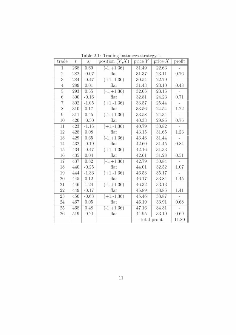
Table 2.1: Trading instances strategy I.trade t st position (Y ,X) price Y price X profit

1 268 0.69 (-1,+1.36) 31.49 22.63 -2 282 -0.07 flat 31.37 23.11 0.763 284 -0.47 (+1,-1.36) 30.54 22.79 -4 289 0.01 flat 31.43 23.10 0.485 293 0.55 (-1,+1.36) 32.05 23.15 -6 300 -0.16 flat 32.81 24.23 0.717 302 -1.05 (+1,-1.36) 33.57 25.44 -8 310 0.17 flat 33.56 24.54 1.229 311 0.45 (-1,+1.36) 33.58 24.34 -10 420 -0.30 flat 40.33 29.85 0.7511 423 -1.15 (+1,-1.36) 40.79 30.82 -12 428 0.08 flat 43.15 31.65 1.2313 429 0.65 (-1,+1.36) 43.43 31.44 -14 432 -0.19 flat 42.60 31.45 0.8415 434 -0.47 (+1,-1.36) 42.16 31.33 -16 435 0.04 flat 42.61 31.28 0.5117 437 0.82 (-1,+1.36) 42.79 30.84 -18 440 -0.25 flat 44.01 32.52 1.0719 444 -1.33 (+1,-1.36) 46.53 35.17 -20 445 0.12 flat 46.17 33.84 1.4521 446 1.24 (-1,+1.36) 46.32 33.13 -22 449 -0.17 flat 45.89 33.85 1.4123 450 -0.63 (+1,-1.36) 45.46 33.87 -24 467 0.05 flat 46.19 33.91 0.6825 468 0.48 (-1,+1.36) 47.16 34.31 -26 519 -0.21 flat 44.95 33.19 0.69

total profit 11.80

11

Rather than closing the position at 0, one could also choose to reverse theposition when the spread reaches Γ in the other direction. Assume we havesold 1 Y and bought 1.36 X, because the spread was larger than Γ, we couldnow wait until the spread reaches −Γ and buy 2 times Y and sell 2 times1.36 X. As a result, we are now left with a portfolio of long 1 Y and short1.36 X. This results in one initial trade and 12 trades reversing the position.Note that the profit of reversing the position is 2Γ, so the total profit is atleast 12 times 2Γ. These trades are shown in table 2.2.

Table 2.2: Trading instances strategy II.trade t st position (Y ,X) price Y price X profit

1 268 0.69 (-1,+1.36) 31.49 22.63 -2 284 -0.47 (+1,-1.36) 30.54 22.79 1.163 293 0.55 (-1,+1.36) 32.05 23.15 1.024 302 -1.05 (+1,-1.36) 33.57 25.44 1.605 311 0.45 (-1,+1.36) 33.58 24.34 1.506 423 -1.15 (+1,-1.36) 40.79 30.82 1.607 429 0.65 (-1,+1.36 ) 43.43 31.44 1.808 434 -0.47 (+1,-1.36) 42.16 31.33 1.129 437 0.82 (-1,+1.36) 42.79 30.84 1.2910 444 -1.33 (+1,-1.36) 46.53 35.17 2.1511 446 1.24 (-1,+1.36) 46.32 33.13 2.5712 450 -0.63 (+1,-1.36) 45.46 33.87 1.8713 468 0.48 (-1,+1.36) 47.16 34.31 1.11

total profit 18.79

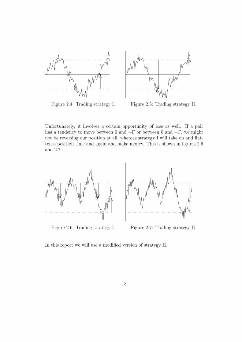
This change of strategy reduces the number of trading instances on averageby a factor of 2. In doing so, we reduce trading costs. More important, if thespread moves around 0 back and forth, strategy II will be more profitable.For example, with the first trade the spread has moved above Γ, so we sell1 Y and buy 1.36 X. When trading according to strategy I, we will flattenour position at 0 and have zero position while moving from 0 to −Γ and notprofit from this movement. When trading according to strategy II, we willstill be short Y and long X while the spread moves to −Γ (eg. X becomesmore expensive relative to Y ). This is shown is figures 2.4 and 2.5.

12

......................................................................................................................................................................

.............................................................................................................................................................................................

...............................................................................................

.......................................................................................................

........................................................................................................................................................................................................................................

........

........

...............................................................................................................................................................................................................................................................................................................................................................................

........

........

........

.......................................................................................................................................................................................................................................................................................................................................................................................................................................................................................................................................................................................................................................................................................................

...............................................................................................................................................................

.................................................................................................................

......................

........

........

........

........

........

........

........

........

........

........

........

.........................

......................

. . . . . . . . . . . . . . . . . . . . . . . . . . . . . . . . . . . . . . . . . . . . . . . . . . . . .

. . . . . . . . . . . . . . . . . . . . . . . . . . . . . . . . . . . . . . . . . . . . . . . . . . . . .

f

f

f

f

f

Figure 2.4: Trading strategy I.

......................................................................................................................................................................

.............................................................................................................................................................................................

...............................................................................................

.......................................................................................................

........................................................................................................................................................................................................................................

........

........

...............................................................................................................................................................................................................................................................................................................................................................................

........

........

........

.......................................................................................................................................................................................................................................................................................................................................................................................................................................................................................................................................................................................................................................................................................................

...............................................................................................................................................................

...........................................................................................................................................................................................................

......................

........

........

........

........

........

........

........

........

........

........

........

........

........

........

........

........

........

........

........

........

........

........

...........................

......................

. . . . . . . . . . . . . . . . . . . . . . . . . . . . . . . . . . . . . . . . . . . . . . . . . . . . .

. . . . . . . . . . . . . . . . . . . . . . . . . . . . . . . . . . . . . . . . . . . . . . . . . . . . .

f

f

f

Figure 2.5: Trading strategy II.

Unfortunately, it involves a certain opportunity of loss as well. If a pairhas a tendency to move between 0 and +Γ or between 0 and −Γ, we mightnot be reversing our position at all, whereas strategy I will take on and flat-ten a position time and again and make money. This is shown in figures 2.6and 2.7.

.............................................................................................................................................................................................................................................................................................................................................................................................................................................................................................

....................................................................................................................................................................................................................................................................................................................................................................................................................................................................................................................................................................................................................................................................................................................................................................................................................................................................................................................................................................................................................................................

........

........

.............................................................................................................................................................................................................................................................................................................................................................................................................................................................................................................................................................................................................................................................................................................................................................................................................................................................................................................................................................................................................................

...........................................................................................................................................................................................................................................................................................................................................................

........

........

........

........

........

.......................................................................................................................................................................................................................................................................................................................................................................................................................................................................................................................

.................................................................................................................

......................

.................................................................................................................

......................

.................................................................................................................

......................

........

........

........

........

........

........

........

........

........

........

........

.........................

......................

. . . . . . . . . . . . . . . . . . . . . . . . . . . . . . . . . . . . . . . . . . . . . . . . . . . . . . .

. . . . . . . . . . . . . . . . . . . . . . . . . . . . . . . . . . . . . . . . . . . . . . . . . . . . . . .

f

f

f

f

f

f

f

f

Figure 2.6: Trading strategy I.

.............................................................................................................................................................................................................................................................................................................................................................................................................................................................................................

....................................................................................................................................................................................................................................................................................................................................................................................................................................................................................................................................................................................................................................................................................................................................................................................................................................................................................................................................................................................................................................................

........

........

.............................................................................................................................................................................................................................................................................................................................................................................................................................................................................................................................................................................................................................................................................................................................................................................................................................................................................................................................................................................................................................

...........................................................................................................................................................................................................................................................................................................................................................

........

........

........

........

........

.......................................................................................................................................................................................................................................................................................................................................................................................................................................................................................................................

...........................................................................................................................................................................................................

......................

. . . . . . . . . . . . . . . . . . . . . . . . . . . . . . . . . . . . . . . . . . . . . . . . . . . . . . .

. . . . . . . . . . . . . . . . . . . . . . . . . . . . . . . . . . . . . . . . . . . . . . . . . . . . . . .

f

f

Figure 2.7: Trading strategy II.

In this report we will use a modified version of strategy II.

13

2.2 Data

The price data which IMC uses is provided by Bloomberg. Bloomberg is aleading global provider of data, news and analytic tools. Bloomberg providesreal-time and archived financial and market data, pricing, trading, news andcommunications tools in a single, integrated package to corporations, newsorganizations, financial and legal professionals and individuals around theworld.

Historical closing prices of stocks are easily extracted from Bloomberg toExcel. One issue has to be considered, namely dividend. Companies nor-mally pay out dividend to its shareholders every year or twice a year, somecompanies pay out dividend four times a year. The amount of dividend issubtracted from the stock price at the day the dividend is paid out, calledgoing ex-dividend. This usually results in a twist in the price process like inpicture 2.8.

40

45

50

55

60

¿

..........................................................................................................................................................

.......................................................................................................................................

............................................................................................................................................................................................................................

................................................................................

.............................................................................................

....................................................................

...............................................

t

Figure 2.8: Dividend.

It is unlikely that different companies go ex-dividend at the same day. Sothe closing prices of stocks have to be corrected for dividend, to make a goodcomparison with other stocks. In this report we will assume that the divi-dend is re-invested in the stock. So it is not just adding the dividend up withthe closing price, it is a growing amount proportionally to the growth of thestock price.

14

Example Consider the following the ex-dividend dates and amounts of acertain stock.

date amount04/28/2003 1.2004/30/2004 1.4004/29/2005 1.70

Suppose we want to use data of this stock starting from 03/01/2004. So weextract from Bloomberg the closing prices from this date forward, actuallywe start at 03/02/2004 because the first of March was a Sunday. From03/02/2004 until 04/29/2004 we use exactly these prices, the first ex-dividendis not used. On 04/30/20004 the stock is ex-dividend for the amount of 1.40.We calculate what percentage this is of the stock price and from this dateforward we keep multiplying the closing prices from Bloomberg with thispercentage until the next ex-dividend date. Then we calculate the percentageof the dividend amount and adding it up to the percentage before, this isshown in table 2.3.

2.3 Properties of pairs trading

Pairs trading is almost cash neutral, we do not have to invest a lot of money.We use the earnings of short selling one stock to purchase the other stock.This usually does not exactly sum up to zero, to be precise it sums up to ±Γ,a small positive or negative amount compared to the stock prices. An otheraspect that makes pairs trading not entirely cash neutral is short selling.Short selling is selling something we do not have. The exchange on whichwe trade will want to be sure that we will not go bankrupt. We need to putmoney, called margin, aside to secure the exchange there are no risks involvedwith short selling. Normally, this margin is a percentage of the value of theshort sale, typically between 5 and 50, depending on the credibility of theshort seller. IMC’s costs for short selling are relatively low, so pairs tradingis almost cash neutral.

15

Table 2.3: Calculation of closing prices corrected for dividend.

date Bloomberg dividend factor our prices03/02/2004 44.00 - 1 44.0003/03/2004 43.37 - 1 43.37

......

......

...04/29/2004 43.85 - 1 43.8504/30/2004 43.04 1.40 1+1.40/43.04=1.03 1.03*43.04=44.3305/01/2004 42.90 - 1.03 1.03*42.90=44.19

......

......

...4/28/2005 51.44 - 1.03 1.03*51.44=52.984/29/2005 50.11 1.70 1.03+1.70/50.11=1.07 1.07*50.11=53.624/30/2005 50.64 - 1.07 1.07*50.64=54.18

......

......

...

Pairs trading is also market neutral: if the overall market goes up 10% ithas no consequences for the strategy and profits of pairs trading. The 10%loss in the short stock is compensated by a 10% gain in the long stock, andthe other way around if the overall market goes down. We do not have apreference for up or down movements, we only look at relative pricing.

How to make money with pairs trading was explained in the example inparagraph 2.1. The amount of money made by trading a pair is a measurefor the quality of a pair. Obviously, more money is better! We make profitsif the spread oscillates around zero often hitting Γ and −Γ. An importantissue for the traders is that the spread should not be away from zero for along time. Traders are humans and they tend to get a bit nervous if theyhave a big position for a long time. There is a chance that the spread willnever return to zero and in that case it costs money to flatten the position.

Example Consider figure 2.9 of the spread of pair X, Y . We put on a po-sition the first time the spread hits −Γ, because there Y is cheap relative toX in our opinion. We reverse our position at +Γ and again at −Γ, makinga profit of at least 4Γ. Then we like the spread to go to +Γ, but the spreadis going further and further away from zero not knowing if it will ever come

16

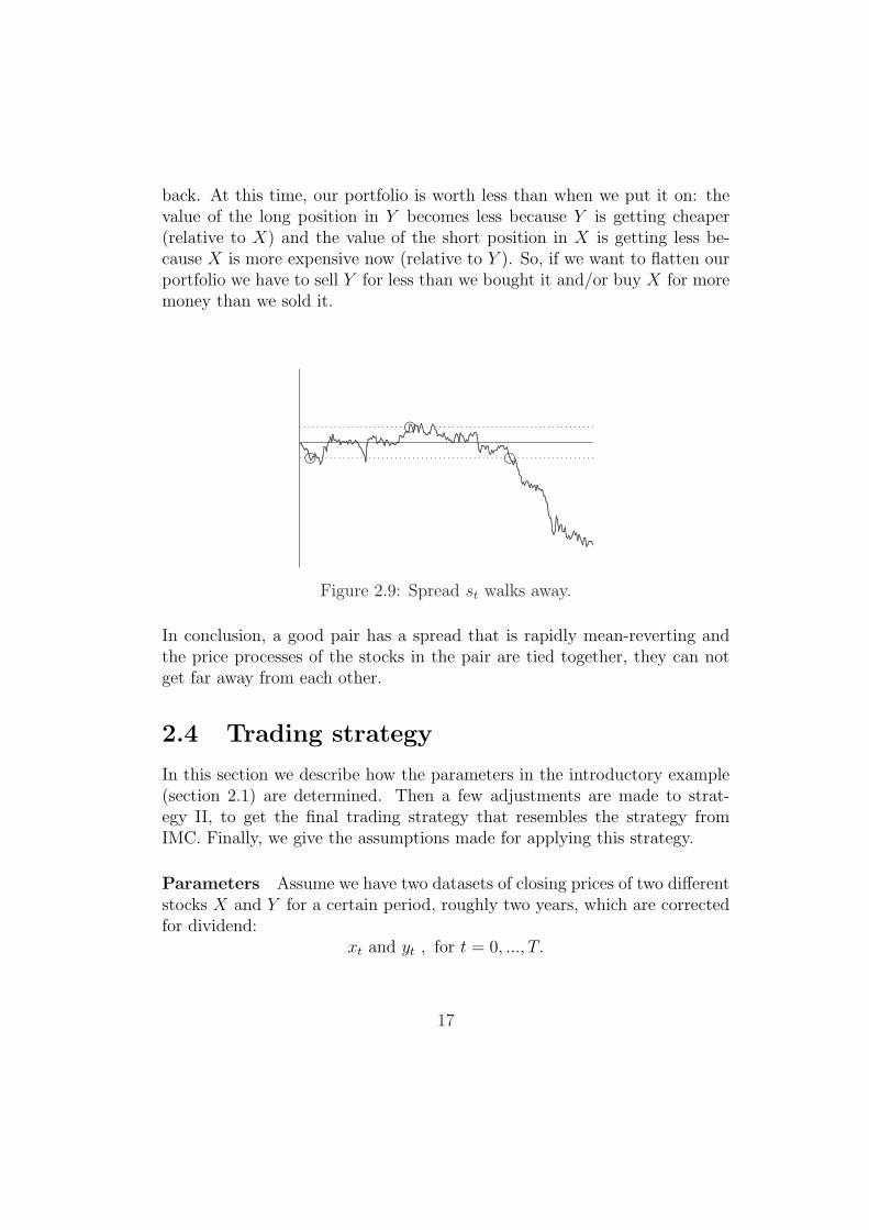
back. At this time, our portfolio is worth less than when we put it on: thevalue of the long position in Y becomes less because Y is getting cheaper(relative to X) and the value of the short position in X is getting less be-cause X is more expensive now (relative to Y ). So, if we want to flatten ourportfolio we have to sell Y for less than we bought it and/or buy X for moremoney than we sold it.

.................................................................................................

...................................................................................................................................................................................................................................

........

........

.........

....................................................

.....................................................................

............................................................................................................................................................

......................................................................................................

.............................................................................

..........................................................................................................................................

..................................................................................................................................................

........................................................................................................................................................................

........

........

....................................................................................................................

......................................................................................................................

. . . . . . . . . . . . . . . . . . . . . . . . . . . . . . . . . . . . . . . . . . . . . . . . . . . . . . . . . . . . . . . . . . . .

. . . . . . . . . . . . . . . . . . . . . . . . . . . . . . . . . . . . . . . . . . . . . . . . . . . . . . . . . . . . . . . . . . . .ff

f

Figure 2.9: Spread st walks away.

In conclusion, a good pair has a spread that is rapidly mean-reverting andthe price processes of the stocks in the pair are tied together, they can notget far away from each other.

2.4 Trading strategy

In this section we describe how the parameters in the introductory example(section 2.1) are determined. Then a few adjustments are made to strat-egy II, to get the final trading strategy that resembles the strategy fromIMC. Finally, we give the assumptions made for applying this strategy.

Parameters Assume we have two datasets of closing prices of two differentstocks X and Y for a certain period, roughly two years, which are correctedfor dividend:

xt and yt , for t = 0, ..., T.

17

The first half, t = 0, ..., bT/2c, is considered as history and is used to deter-mine the parameters ratio r and threshold Γ.

The second half, t = bT/2c + 1, ..., T , is considered as the future and isused to determine the profit or loss that would be made trading the pairX,Y with these parameters.

The ratio r is the average ratio of Y and X of the first half of observations:

r =1

bT/2c+ 1

bT/2c∑t=0

xt

yt

.

The threshold Γ is determined quite easily, we just try a few on the ’history’and take the one that gives the best profit based on the ’history’. We calculatethe maximum of the absolute spread of the first half of observations, denotedas m:

m = maxt

(|yt − rxt|, t = 0, ..., bT/2c).The values of Γ that we are going to try are percentages of m. Table 2.4shows the percentages and the outcome for the introductory example of para-graph 2.1, where m = 2.01. Because of rounding to two digits it looks likethere are several values of Γ which give the same largest profit, but Γ = 0.40gives the largest profit.

The profit is calculated by multiplying number of trades minus one withtwo times Γ, except when no trades were made then the profit is just zero.It is the minimal profit if you always trade one spread, in this example oneY and 1.36 X. The first trading instance is to put on a position for the firsttime, denoted by t1, then we do not make a profit yet:

t1 = min (t, such that |st| ≥ Γ).

The succeeding trading moments are:

If stn ≥ Γ:tn+1 = min (t, such that t > tn, st ≤ −Γ).

If stn ≤ −Γ:tn+1 = min (t, such that t > tn, st ≥ Γ).

18

Table 2.4: Profits with different Γ.

percentage Γ trades profit5 0.10 15 2.8110 0.20 9 3.2115 0.30 9 4.8220 0.40 7 4.8225 0.50 3 2.0130 0.60 3 2.4135 0.70 3 2.8140 0.80 3 3.2145 0.90 3 3.6150 1.00 3 4.0255 1.10 3 4.4260 1.20 3 4.8265 1.30 2 2.6170 1.40 2 2.8175 1.51 2 3.0180 1.61 2 3.2185 1.71 1 090 1.81 0 0

To determine Γ we simply take the one that has the largest profit basedon the history, but in practice we do not take Γ larger than 0.5m. Thisprofit is a gross profit, no transaction costs are accounted. We neglectedthe transaction costs because it turned out they hardly had any influence onthe value of Γ. This is because IMC does not trade one spread, which inthis example was 1 Y and 1.36 X, but they trade a large number of Y andX, for example 1,000 Y and 1,360 X. The costs that IMC makes consistsof two parts, a fixed amount a plus amount b times the number of tradedstocks. The costs of trading 1,000 Y and 1,360 X would be 2a + 2, 360b. Wealways trade the same amount, no matter the value of Γ, so the costs pertrade for all Γ are exactly the same. So the more trades the more costs, butthe costs are really small compared to the profit. When the profits for thedifferent thresholds are not too close to each other, the Γ when considering

19

the net profits is the same Γ when neglecting the costs. Unfortunately of allthe pairs considered in this report, the pair from table 2.4 is the only onewhere accounting transaction costs would have made a difference. There arethree thresholds, 0.30, 0.40 and 1.20, which result in almost the same profits.Therefor accounting the transaction costs would resulted in the thresholdwith the lowest number of trades, Γ = 1.20. In the remainder of this report,we will neglect transaction costs.

Modified trading strategy There are pairs of stock that work quite wellfor a certain time but then the spread walks away from zero and starts tooscillate around a level different from zero. We can see an example in fig-ure 2.10. If we do not do anything, we are probably going to have a positionfor a long time which is not desirable as explained in paragraph 2.3. Thefigure shows us that the relation between the stocks in the pair has changed,the ratio r, determined by the past, is not good anymore. It would be a wasteto lose money on these kind of pairs by closing the position or to excludethem from trading. A better way is to replace the average ratio r with somekind of moving average ratio.

0 100 200 300 400 500−5

0

5

..............................................................................................................................................................................................................................................................

..................................................................................................................................................................................................................................................................................

.................................................................................................................................................................................................................................................................................

.................................................................................................................................................................................................................................................................................................................................................................................................................................................................................................................................................................................................................

...........................................................................................................................................................................................

...............................................................................................................................................................................................................................................................................................................................................................................................................................................................................................................................................................................................................................................................................................................................................................................................................

........

........

........

..........................................................................................................................................................................................................................................................................................................................................................................................................................................................................................................................................................................................................................................................................................................................................................................................................................................................................................................................................................................................................................................................................................................................................

.........

.........

........

..............................................................................................................................................................................................

.........

............................................................................................................................................................................................................................................................................

.................................................................................................................................................................................................................................................................................................................................................................................................................................................................................................................................................................................................

. . . . . . . . . . . . . . . . . . . . . . . . . . . . . . . . . . . . . . . . . . . . . . . . . . . . . . . . . . . . . . . . . . . . . . . . . . . . .

. . . . . . . . . . . . . . . . . . . . . . . . . . . . . . . . . . . . . . . . . . . . . . . . . . . . . . . . . . . . . . . . . . . . . . . . . . . . .

Figure 2.10: Spread oscillates around a new level.

Assume we have a dataset of closing prices, the first half is used in the exactsame way as described before. So we have the average ratio r and threshold Γ.The backtest on the second half of the data set is slightly different becausewe use a moving average ratio rt, instead of r, to calculate the spread.

20

The moving average ratio we use, is:

rt = (1− κ) rt−1 + κ rt, t = bT/2c+ 1, ..., T,

with rbT/2c = r and where rt is the actual ratio:

rt =yt

xt

, t = 0, ..., T.

The parameter κ is a percentage between 0 and 10% and is determined verysimple with the first half of the data set. We count how many trades weremade in the first half and use table 2.5 to find κ.

Table 2.5: Determining κ.

# trades κ # trades κ>15 0 4 610-15 1 3 78,9 2 2 87 3 1 96 4 0 105 5

If there were a lot of trades in the first half of observations we do not expectto need a moving average ratio, the table motivates this. The use of a movingaverage ratio and this way of determining its value, has some disadvantageswhich will be discussed later on.

So the first half of the data set determines three parameters: Average ratio r,threshold Γ and adjustment parameter κ. In the second half of the data set,the new spread is calculated as:

sκ, t = yt − rtxt.

Trading the pair goes in the same way as described before, the differenceis the position in X is not equal to r anymore but it is equal to rt. Thefollowing example will make this more clear.

21

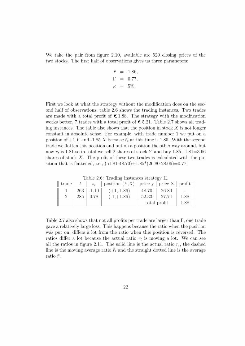
We take the pair from figure 2.10, available are 520 closing prices of thetwo stocks. The first half of observations gives us three parameters:

r = 1.86,

Γ = 0.77,

κ = 5%.

First we look at what the strategy without the modification does on the sec-ond half of observations, table 2.6 shows the trading instances. Two tradesare made with a total profit of ¿ 1.88. The strategy with the modificationworks better, 7 trades with a total profit of ¿ 5.21. Table 2.7 shows all trad-ing instances. The table also shows that the position in stock X is not longerconstant in absolute sense. For example, with trade number 1 we put on aposition of +1 Y and -1.85 X because rt at this time is 1.85. With the secondtrade we flatten this position and put on a position the other way around, butnow rt is 1.81 so in total we sell 2 shares of stock Y and buy 1.85+1.81=3.66shares of stock X. The profit of these two trades is calculated with the po-sition that is flattened, i.e., (51.81-48.70)+1.85*(26.80-28.06)=0.77.

Table 2.6: Trading instances strategy II.trade t st position (Y,X) price y price X profit

1 263 -1.10 (+1,-1.86) 48.70 26.80 -2 285 0.78 (-1,+1.86) 52.33 27.74 1.88

total profit 1.88

Table 2.7 also shows that not all profits per trade are larger than Γ, one tradegave a relatively large loss. This happens because the ratio when the positionwas put on, differs a lot from the ratio when this position is reversed. Theratios differ a lot because the actual ratio rt is moving a lot. We can seeall the ratios in figure 2.11. The solid line is the actual ratio rt, the dashedline is the moving average ratio rt and the straight dotted line is the averageratio r.

22

Table 2.7: Trading instances modified strategy.trade t sκ, t position (Y,X) price Y price X rt profit

1 263 -0.99 (+1,-1.85) 48.70 26.80 1.85 -2 281 1.07 (-1,+1.81) 51.81 28.06 1.81 0.773 358 -0.82 (+1,-1.97) 51.52 26.56 1.97 -2.434 392 0.93 (-1,+1.96) 56.38 28.23 1.96 1.575 407 -0.94 (+1,-1.98) 55.45 28.52 1.98 1.526 459 0.97 (-1,+1.98) 55.27 27.47 1.98 1.927 476 -1.31 (+1,-1.99) 57.20 29.38 1.99 1.86

total profit 5.21

300 350 400 450 5001.7

1.8

1.9

2.0

2.1

.....................................................................................................................................................................................................................................................................................................................................................................................................................................................................................................................................................................................................................................................

.............................................................................................................................................................................................................................................................................................................................

.........

........

........

................................................................................................................................................................................................................................................................................................................................................................................................................

.........

........

............................................................................................................

........

................................................................................................................................................................................................

........

....................................................................................................................................................

........

........

............................................................................................................................................................................................................................................................

...........................................................................................................................................................................................................................................

......................................................................................................................................................................................................................

............................................................

....................................................................................................................................

...................................

...............................

.........................................................................................................................................................................

.....................................................................................

. . . . . . . . . . . . . . . . . . . . . . . . . . . . . . . . . . . . . . . . . . . . . . . . . . . . . . . . . . . . . . . . . . . . . . . . . .

Figure 2.11: Ratios rt, rt and r.

23

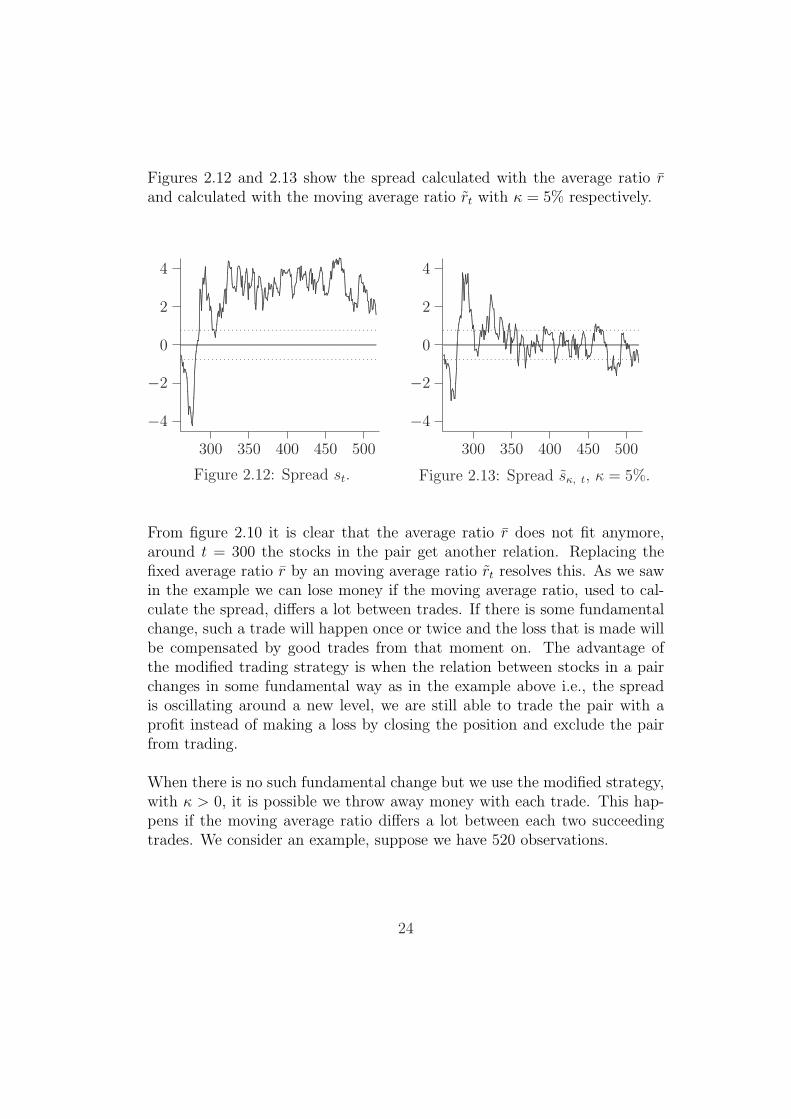
Figures 2.12 and 2.13 show the spread calculated with the average ratio rand calculated with the moving average ratio rt with κ = 5% respectively.

300 350 400 450 500

−4

−2

0

2

4

...........................................................................................................................................................................................................................................................................................................................................................................................................................................................................................................................................................................................................................................................................................................................................................................................................................................................................................................................................................................................................................................................................................................................................................................................................................

.........

........

........

........

................................................................................................................................................................................................................................................................................................................................................................................................................................................................................................................................................................................................................................................................................................................................................................................................................................................................................................................................................................................................................................................................................................................................................................................................................................................................................................................................................................................................................................................................................................................................................................................................................................................................................................................................................................................................

.........

.........................................................................................................................................................................................................................................................................................................................................................................................

.................................................................................................................................................................................................................................................................................................................................................................................

. . . . . . . . . . . . . . . . . . . . . . . . . . . . . . . . . . . . . . . . . . . . . . . . . .

. . . . . . . . . . . . . . . . . . . . . . . . . . . . . . . . . . . . . . . . . . . . . . . . . .

Figure 2.12: Spread st.

300 350 400 450 500

−4

−2

0

2

4

..............................................................................................................................................................................................................................................................................................................................................................................................................................................................................................................................................................................................................................................................................................................................................................................................

.........

........

.........

........

...................................................................................................................................................................................................................................................................................................................................................

.........

........

........

........

.....................................................................................................................................................................................................................................................................................................................................................................................................................................................................................................................................................................................................................................................................................................................................................................................................................................................................................................................................

..........................................................................................................................................................................................................................................................................................................................................................................................................................................................................................................................................................................................................................................................................................................................................................................................................................

.........

........

........................................................................................................................................................................................................................................................................................................................................................................

.................................................................................................................................................................................................................................................................................................................................................................................

. . . . . . . . . . . . . . . . . . . . . . . . . . . . . . . . . . . . . . . . . . . . . . . . . .

. . . . . . . . . . . . . . . . . . . . . . . . . . . . . . . . . . . . . . . . . . . . . . . . . .

Figure 2.13: Spread sκ, t, κ = 5%.

From figure 2.10 it is clear that the average ratio r does not fit anymore,around t = 300 the stocks in the pair get another relation. Replacing thefixed average ratio r by an moving average ratio rt resolves this. As we sawin the example we can lose money if the moving average ratio, used to cal-culate the spread, differs a lot between trades. If there is some fundamentalchange, such a trade will happen once or twice and the loss that is made willbe compensated by good trades from that moment on. The advantage ofthe modified trading strategy is when the relation between stocks in a pairchanges in some fundamental way as in the example above i.e., the spreadis oscillating around a new level, we are still able to trade the pair with aprofit instead of making a loss by closing the position and exclude the pairfrom trading.

When there is no such fundamental change but we use the modified strategy,with κ > 0, it is possible we throw away money with each trade. This hap-pens if the moving average ratio differs a lot between each two succeedingtrades. We consider an example, suppose we have 520 observations.

24

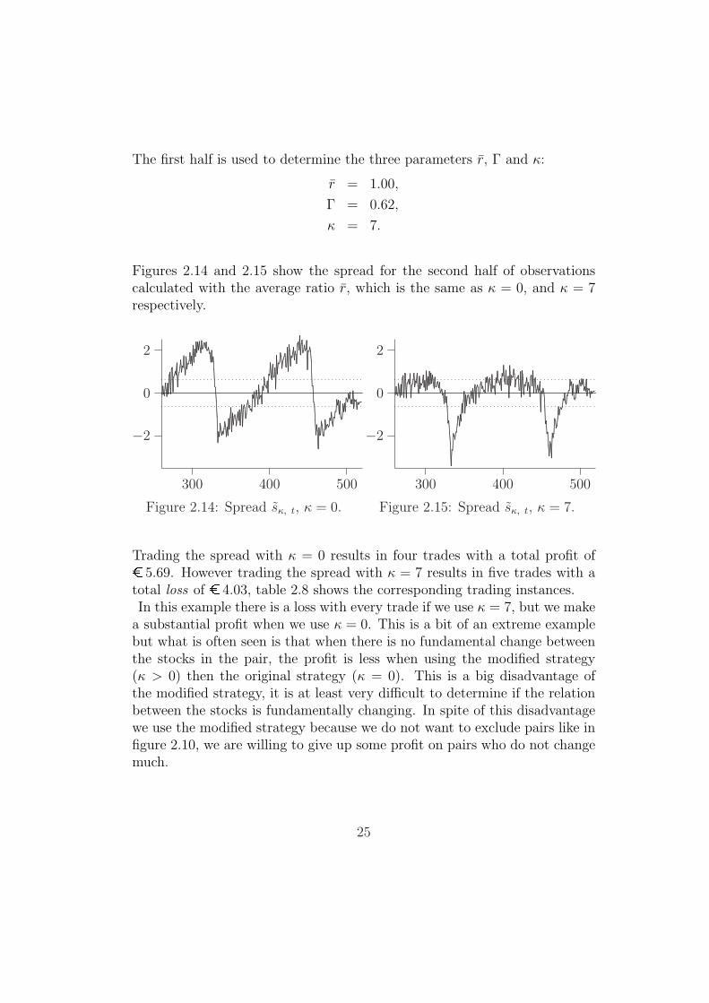
The first half is used to determine the three parameters r, Γ and κ:

r = 1.00,

Γ = 0.62,

κ = 7.

Figures 2.14 and 2.15 show the spread for the second half of observationscalculated with the average ratio r, which is the same as κ = 0, and κ = 7respectively.

300 400 500

−2

0

2

........

........

....................................................................................................................................................................................................................................................................................................................................................................................................................................................................................................................................................................................................................................................................................................................................................................................................................................................................................................................................................................................................................................................................................................................................................................................................................................................................................................................................................................................................................................................................................................................................................................................................................................................................................................................................................................................................................................................................................................................................................................................................................................................................................................................................................................................................................................................................................................................................................................................................................................................................................................................................................................................................................................................................................................................................................................................................................................................................................................................................................................................................................................................................................................................................................................................................................................................................................................................................................................................................................................................................................................................................................................................................................................................................................................................................................................................................................................................................................................................................................................................................................................................................................................................................................................................................

........

.......................................................................................................................................................................................................................................................................................................................................................................................................................................................................................................................................................................................................................................................................................................................................................................................................................................................................................................

.......................................................................................................................................................................................................................................................................................................................................................................................................................................

. . . . . . . . . . . . . . . . . . . . . . . . . . . . . . . . . . . . . . . . . . . . . . . . . . . . . . . . .

. . . . . . . . . . . . . . . . . . . . . . . . . . . . . . . . . . . . . . . . . . . . . . . . . . . . . . . . .

Figure 2.14: Spread sκ, t, κ = 0.

300 400 500

−2

0

2

........

........

...........................................................................................................................................................................................................................................................................................................................................................................................................................................................................................................................................................................................................................................................................................................................................................................................................................................................................................................................................................................................................................................................................................................................................................................................................................................................................................................................................................................................................................................................................................................................................................................................................................................................................................................................................................................................................................................................................................................................................................................................................................................................................................................................................................................................................................................................................................................................................................................................................................................................................................................................................................................................................................................................................................................................................................................................................................................................................................................................................................................................................................................................................................................................................................................................................................................................................................................................................................................................................................................................................................................................................................................................................................................................................................................................................................................................................................................................................................................................................................................................................................................................................................................................

........

........

.............................................................................................................................................................................................................................................................................................................................................................................................................................................................................................................................................................................................................................................................................................................................................................................................................................................................................................................................................................................................................................................................................................................................................................................................................................................................................................

. . . . . . . . . . . . . . . . . . . . . . . . . . . . . . . . . . . . . . . . . . . . . . . . . . . . . . . . .

. . . . . . . . . . . . . . . . . . . . . . . . . . . . . . . . . . . . . . . . . . . . . . . . . . . . . . . . .

Figure 2.15: Spread sκ, t, κ = 7.

Trading the spread with κ = 0 results in four trades with a total profit of¿ 5.69. However trading the spread with κ = 7 results in five trades with atotal loss of ¿ 4.03, table 2.8 shows the corresponding trading instances.In this example there is a loss with every trade if we use κ = 7, but we make

a substantial profit when we use κ = 0. This is a bit of an extreme examplebut what is often seen is that when there is no fundamental change betweenthe stocks in the pair, the profit is less when using the modified strategy(κ > 0) then the original strategy (κ = 0). This is a big disadvantage ofthe modified strategy, it is at least very difficult to determine if the relationbetween the stocks is fundamentally changing. In spite of this disadvantagewe use the modified strategy because we do not want to exclude pairs like infigure 2.10, we are willing to give up some profit on pairs who do not changemuch.

25

Table 2.8: Trading instances modified strategy.trade t sκ, t position (Y,X) price Y price X rt profit

1 270 0.71 (-1,+1.01) 10.72 9.94 1.01 -2 328 -0.63 (+1,-1.18) 10.80 9.72 1.18 -0.303 378 0.72 (-1,+0.92) 9.93 10.50 0.92 -1.254 449 -0.87 (+1,-1.18) 11.59 10.55 1.18 -1.215 487 0.63 (-1,+0.90) 9.54 9.88 0.90 -1.27

total profit -4.03

Assumptions We apply the trading strategy to historical closing data tosee if trading a pair of two stocks would have been profitable. This assumesthat we could have traded on the closing price and that there was no bid-ask spread. It also assumes we could have traded every amount we wanted,including fractions. If it is decided to start trading a specific pair, it is goingto be traded intra-day, so it would probably be better to apply the tradingstrategy to intra-day data but that kind of data is difficult to get and isdifficult to handle. With real life trading the number of stocks have to beintegers. The assumption that we are allowed to trade fractions is not thatbad because when trading a pair it is about large quantities so we can roundthe number of stocks to an integer without completely messing up the ratios.

2.5 Conclusion

In this chapter we have derived a trading strategy that resembles the strategyIMC uses. It is not necessary anymore to do a fundamental analysis to findout if a pair of two stocks is profitable to trade as a pair. We can apply thetrading strategy on historical data and see if we would have made a profitif we actually traded the pair. In this way IMC identified a lot of pairs.We would like to see if we can identify pairs in a more statistical setting,again using historical data of two stocks, not to estimate profits, but to see ifthe two time series exhibit behavior that could make them a good pair. Wewill examine the concept of cointegration, but first we need some time seriesbasics.

26

Chapter 3

Time series basics

This chapter discusses briefly some basics of time series which we will needfor later purposes. More information can be found in [2] and [3].

White noise A basic stochastic time series zt is independent white noise,if zt is an independent and identically distributed (i.i.d.) variable with mean0 and variance σ2 for all t, notation zt ∼ i.i.d(0, σ2). A special case is Gaus-sian white noise, where each ut is independent and has a normal distribu-tion N(0, σ2).

Stationarity A time series zt is covariance-stationary or weakly station-ary if neither the expectation nor the autocovariances depend on time t:

E(zt) = µ,

E(zt − µ)(zt−j − µ) = γj,

for all t and j. Notice that if a process is covariance-stationary, the variance ofzt is constant and the covariance between zt and zt−j depends only on lag j.For example, a white noise process is covariance-stationary. Covariance-stationary is shortened by stationary in the remaining of this report.

A stationary process exhibits mean reverting behavior, the process tendsto remain near or tends to return over time to the mean value.

27

MA(q) A q-th order moving average process, denoted MA(q), is character-ized by:

zt = µ + ut + θ1ut−1 + θ2ut−2 + · · ·+ θqut−q, (3.1)

where ut is white noise (∼ i.i.d(0, σ2)), µ and (θ1, θ2, . . . , θq) are constants.The expectation, variance and autocovariances of zt are given by:

E(zt) = µ,

γ0 = (1 + θ21 + θ2

2 + · · ·+ θ2q)σ

2,

γj =

(θj + θj+1θ1 + θj+1θ2 + · · ·+ θqθq−j)σ

2 if j = 1, . . . , q,0 if j > q.

So an MA(q) process is stationary.

AR(1) A first-order autoregressive process, denoted AR(1), satisfies thefollowing difference equation:

zt = c + φzt−1 + ut, (3.2)

where ut is independent white noise (∼ i.i.d(0, σ2)). If |φ| ≥ 1 , the conse-quences of the u’s for z accumulate rather than die out over time. Perhaps itis not surprising that when |φ| ≥ 1, there does not exist a causal stationaryprocess for zt with finite variance that satisfies (3.2). If |φ| > 1 the processzt can be written in terms of innovation in the future instead of innovationsin the past, that is what is meant by ’there does not exist a causal stationaryprocess’. If φ = 1 and c = 0 the process is called a random walk. When|φ| < 1, the AR(1) model defines a stationary process and has an MA(∞)representation:

zt = c/(1− φ) + ut + φut−1 + φ2ut−2 + φ3ut−3 + · · · .

The expectation, variance and autocovariances of zt are given by:

µ = c/(1− φ),

γ0 = σ2/(1− φ2),

γj = (σ2φj/(1− φ2)), for j = 1, 2, . . .

28

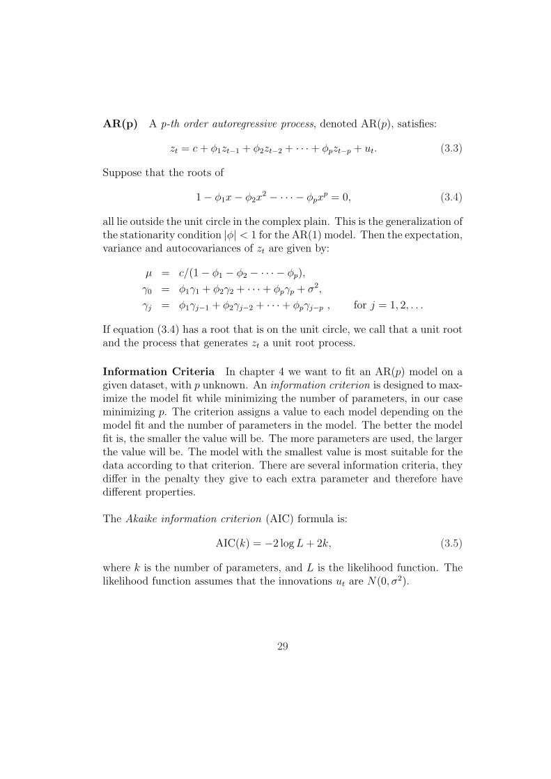
AR(p) A p-th order autoregressive process, denoted AR(p), satisfies:

zt = c + φ1zt−1 + φ2zt−2 + · · ·+ φpzt−p + ut. (3.3)

Suppose that the roots of

1− φ1x− φ2x2 − · · · − φpx

p = 0, (3.4)

all lie outside the unit circle in the complex plain. This is the generalization ofthe stationarity condition |φ| < 1 for the AR(1) model. Then the expectation,variance and autocovariances of zt are given by:

µ = c/(1− φ1 − φ2 − · · · − φp),

γ0 = φ1γ1 + φ2γ2 + · · ·+ φpγp + σ2,

γj = φ1γj−1 + φ2γj−2 + · · ·+ φpγj−p , for j = 1, 2, . . .

If equation (3.4) has a root that is on the unit circle, we call that a unit rootand the process that generates zt a unit root process.

Information Criteria In chapter 4 we want to fit an AR(p) model on agiven dataset, with p unknown. An information criterion is designed to max-imize the model fit while minimizing the number of parameters, in our caseminimizing p. The criterion assigns a value to each model depending on themodel fit and the number of parameters in the model. The better the modelfit is, the smaller the value will be. The more parameters are used, the largerthe value will be. The model with the smallest value is most suitable for thedata according to that criterion. There are several information criteria, theydiffer in the penalty they give to each extra parameter and therefore havedifferent properties.

The Akaike information criterion (AIC) formula is:

AIC(k) = −2 log L + 2k, (3.5)

where k is the number of parameters, and L is the likelihood function. Thelikelihood function assumes that the innovations ut are N(0, σ2).

29

The log likelihood for an AR(k) model is given by:

log L = − T

2log(2π)− T

2log(σ2) +

1

2log |V−1

k |

− 1

2σ2(zk − µk)

′V−1k (zk − µk)

−T∑

t=k+1

(zt − c− φ1zt−1 − · · · − φkzt−k)2

2σ2

where σ2Vk denotes the covariance matrix of (z1, z2, . . . , zk):

σ2Vk =

E(z1 − µ)2 E(z1 − µ)(z2 − µ) · · · E(z1 − µ)(zk − µ)E(z2 − µ)(z1 − µ) E(z2 − µ)2 · · · E(z2 − µ)(zk − µ)

...... · · · ...

E(zk − µ)(z1 − µ) E(zp − µ)(z2 − µ) · · · E(zk − µ)2

and µk denotes a (k × 1) vector with each element given by

µ = c/(1− φ1 − φ2 − · · · − φk),

and zk denotes the first k observations in the sample, (z1, z2, . . . , zk) and Tdenotes the sample size.

The first term in (3.5) measures the model fit, the second term gives a penaltyto each parameter. The Akaike information criterion is calculated for eachmodel AR(k), with k = 1, 2, . . . , K. The k with the smallest value AIC(k),is the estimate for the model order.

Two other information criteria are the Schwarz-Baysian and the Hannan-Quint information criteria.

The Schwarz-Baysian information criterion (BIC) formula is:

BIC(k) = −2 log L + k log(T ),

where T denotes the number of observations in the data set.

The Hannan-Quint information criterion (HIC) formula is:

HIC(k) = −2 log L + 2k log(log(T )).

30

First difference operator The first difference operator ∆ is defined by:

∆zt = zt − zt−1.

I(d) A time series is integrated of order d, written as yt ∼ I(d), if the seriesis non-stationary but it becomes stationary after differencing a minimumof d times. An already weakly stationary process is denoted as I(0). If atime series generated by an AR(p) process is integrated of order d, than itsautoregressive polynomial (equation (3.4)) has d roots on the unit circle.

Unit root test Statistical tests of the null hypothesis that a time seriesis non-stationary against the alternative that it is stationary are called unitroot tests. In this paper we consider the Dickey-Fuller test (DF) and theAugmented Dickey-Fuller test (ADF).

Dickey-Fuller test The Dickey-Fuller test tests whether a time series isstationary or not when the series is assumed to follow an AR(1) model. It isnamed after the statisticians D.A. Dickey and W.A. Fuller, who developedthe test in [4].

The assumption of the DF test is that the time series zt follows an AR(1)model:

zt = c + ρzt−1 + ut, (3.6)

with ρ ≥ 0. If ρ = 1, the series zt is non-stationary. If ρ < 1, the series zt isstationary. The null hypothesis is that zt is non-stationary, more specific zt

is integrated of order 1, against the alternative zt is stationary:

H0 : zt ∼ I(1) against H1 : zt ∼ I(0),

which can be restated in terms of the parameters:

H0 : ρ = 1 against H1 : ρ < 1,

under the assumption that zt follows an AR(1) model.

31

The test statistic of the DF test S is the t ratio:

S =ρ− 1

σρ

,

where ρ denotes the OLS estimate of ρ and σρ denotes the standard error forthe estimated coefficient.

The t ratio is commonly used to test whether the coefficient ρ is equal toρ0 when the time series is stationary, i.e. ρ < 1. Then the test statistic

ρ− ρ0

σρ

,

has a t-distribution. But we do not assume that the time series is stationary,because the null hypothesis is that ρ = 1. So, the test statistic S does notneed to have a t-distribution. We need to distinguish several cases to derivethe distribution of the DF test statistic.

Case 1 :The true process of zt is a random walk, i.e. zt = zt−1 + ut, and we estimatethe model zt = ρzt−1+ut. Notice that we only estimate ρ and not a constant c.

Case 2 :The true process of zt is again a random walk and we estimate the modelzt = c + ρzt−1 + ut. Notice that now we do estimate a constant but it is notpresent in the true process.

Case 3 :The true process of zt is a random walk, but now with drift, i.e. zt =c + zt−1 + ut, where the true value of c is not zero. We estimate the modelzt = c + ρzt−1 + ut.

Although the differences between the three cases seem small, the effect onthe asymptotic distributions of the test statistic are large, as we will see inchapter 5.

32

Augmented Dickey-Fuller test The Augmented Dickey-Fuller test testswhether a time series is stationary or not when the time series follows anAR(p) model. One of the assumptions of the Augmented Dickey-Fuller testis that the time series zt follows an AR(p) model:

zt = c + φ1zt−1 + · · ·+ φpzt−p + ut. (3.7)

Like the regular Dickey-Fuller test, we test:

H0 : zt ∼ I(1) against H1 : zt ∼ I(0).

The null hypothesis is that the autoregressive polynomial

1− φ1x− φ2x2 − · · · − φpx

p = 0,

has exactly one unit root and all other roots are outside the unit circle.Then the unit root cannot be a complex number, because the autoregressivepolynomial is a polynomial with real coefficients and if x = a + bi is a unitroot than so is its complex conjugate x = a − bi. This contradicts the nullhypothesis that there is exactly one unit root. Two possibilities remain, theunit root is -1 or 1. The first possibility gives an alternating series, which isnot realistic for modeling the spread (this becomes more clear in the chapterof cointegration). Thus the single unit root should be equal to 1, which givesus

1− φ1 − φ2 − · · · − φp = 0. (3.8)

The AR(p) model (3.7) can be written as:

zt = c + ρzt−1 + β1∆zt−1 + · · ·+ βp−1∆zt−p+1 + ut, (3.9)

with

ρ = φ1 + · · ·+ φp,

βi = −(φi+1 + · · ·+ φp), for i = 1, . . . , p− 1.

The advantage of writing (3.7) in the equivalent form (3.9) is that underthe null hypothesis only one of the regressors, namely zt−1, is I(1), whereasall of the other regressors (∆zt−1, ∆zt−2, . . . , ∆zt−p+1) are stationary. Notice

33

that (3.8) implies that coefficient ρ is equal to 1. This leads to the samehypotheses as with the regular Dickey-Fuller test:

H0 : ρ = 1 against H1 : ρ < 1,

and the same test statistic:

S =ρ− 1

σρ

.

To derive the distribution of the ADF test statistic we need to distinguishthe same three cases as above, but now in the appropriate AR(p) form. Aswe will see in chapter 5, the distributions are the same as DF distributionswithout any corrections for the fact that lagged values of ∆y are included inthe regression.

One last note: If the null hypothesis that zt is non-stationary cannot berejected, it does not necessarily mean that zt is generated by a I(1) pro-cess. It may be non-stationary because it is generated by a I(2) processor by an integrated process of an even higher order. The next step couldbe to repeat the procedure but this time using ∆yt instead of yt. That is,to test H0 : ∆yt ∼ I(1) against H1 : ∆yt ∼ I(0) which is equivalent toH0 : yt ∼ I(2) against H1 : yt ∼ I(1), and so on.

34

Chapter 4

Cointegration

Empirical research in financial economics is largely based on time series.Ever since Trygve Haavelmos work it has been standard to view economicand financial time series as realizations of stochastic processes. This ap-proach allows the model builder to use statistical inference in constructingand testing equations that characterize relationships between economic andfinancial variables. The Nobel Prize of 2003 for economics has rewarded twocontributions, the ARCH model and cointegration from Robert Engle andClive Granger.

This chapter discusses the concept of cointegration and two methods for test-ing for cointegration, the Engle-Granger and the Johansen method. Othermethods are described in, for example, [13] and [14]. In the last sectionof this chapter a start is made with an alternative method. In this reportthis alternative method is used for generating cointegrated data but not fortesting for cointegration, although this is possible.

4.1 Introducing cointegration

An (n × 1) vector time series yt is said to be cointegrated if each of the seriestaken individually is I(1), integrated of order one, while some linear com-bination of the series a′yt is stationary for some nonzero (n × 1) vector a,named the cointegrating vector.

35

Cointegration means that although many developments can cause permanentchanges in the individual elements of yt, there is some long-run equilibriumrelation tying the individual components together, represented by the linearcombination a′yt.

A simple example of a cointegrated vector process with n = 2, which wastaken from [1], is:

xt = wt + εx, t ,

yt = wt + εy, t ,

wt = wt−1 + εt ,

where error processes εx,t, εy,t and εt are independent white noise processes.The series wt is a random walk, so xt and yt are I(1) processes, though thelinear combination yt − xt is stationary. This means yt = (xt, yt) is cointe-grated with a = (−1, 1).

Figure 4.1 shows a realization of this example of a cointegrated process, wherethe error processes are standard Gaussian white noise. Note that xt and yt

can wander arbitrarily far from the starting value, but xt and yt themselvesare ’tied together’ in the long run. The figure also shows the correspondingspread yt − xt of the realization.

.................................................................................................................................................................................................................................................................................................................................................................................................................................................................................................................................

........

........

........

...........................................................................................................................................................................................................................................................................................................................................................................................................................................................................................................................

.....................................................................................................................................................

..........................................................................

.................................................................................................................................................................................................................................................................................................................................................................................................................

........

........

........

........

........

.........

........

........

........

...............................................................................

........

........

........

........

.........

........

........

........

........

........

................................................................................................................................................................................................................................................

................................................

...................................................

..

..

..

.............................................

.............................................................................

..................

.........................................

.......................................

.....................................................

..

..

..

...................................

..

..

.........

........

........

........

........

........

........

........

.........................................................................................................................................................................................................................................................................................................................................................................................................................................................................................................................................................................................................................................................................................................................................................................................................................................................................................................................................................................................................................................................................................................................................................................................................................................................................................................................................................................................................................................................................................................................................................................................................................................................................................................................................................................................................................................................................................................................................................................................................................................................................................................................................................................................................................................................................................................................................................................................................................................................................................................................................................................................................................................................................................................................................................................................................................................................................................................................................................................................................................................................................................................................................................

........

........

........

........

........

........

........

........................................................................................................................................................................................................................................................................................................................................................................................................................................................................................................................................................................................................................................................................................................................................................................................................................................................................................................................................................................................................................................................................................................................................................................................................................................................................................................................................................................................................................................................................................................................................................................................................................................................................................................................................................................................................................................................................................................................................................................................................................................................................................................................................................................................................................................................................................................................................................................................................................................................................................................................................................................................................................................................................................................................................................................................................................

..................................................................................................................................................................................................................................................................................................................................................................................................................................................

Figure 4.1: Realization of cointegrated process and spread of realization.

36

Correlation Correlation is used in analysis of co-movements in assets butalso in analysis of co-movements in returns. Correlation measures the strengthand direction of linear relationships between variables. If xt denotes a priceprocess of a stock, the returns ht are defined by

ht =xt − xt−1

xt−1

,

with log(1 + ε) ≈ ε as ε → 0, we can approximate this by:

xt − xt−1

xt−1

=xt

xt−1

− 1 ≈ log

(xt

xt−1

).

Correlation can refer to co-movement in the stock returns and in the stockprices themselves, cointegration refers to co-movements in the stock pricesthemselves or the logarithm of the stock prices. Cointegration and correla-tion are related, but they are different concepts. High correlation does notimply cointegration, and neither does cointegration imply high correlation.In fact, cointegrated series can have correlations that are quite low at times.For example, a large and diversified portfolio of stocks which are also inan equity index, where the weights in the portfolio are determined by theirweights in the index, should be cointegrated with the index itself. Althoughthe portfolio should move in line with the index in the long term, there willbe periods when stocks in the index that are not in the portfolio have excep-tional price movements. Following this, the empirical correlations betweenthe portfolio and the index may be rather low for a time.

The simple example at the beginning of this section shows the same, thatis, cointegration does not imply high correlation. For illustration purposes itis convenient to look at the differences, ∆xt and ∆yt, instead of the returnsor xt and yt themselves because in this example they do not have constantvariances. The variance of ∆xt is

Var(∆xt) = Var(xt − xt−1)

= Var(εt + εx, t + εx, t−1)

= σ2 + 2σ2x,

where σ2, σ2x, and σ2

y denote the variances of εt, εx, t and εy, t respectively.

37

In the same way, Var(∆yt) = σ2 + 2σ2y. The covariance of ∆xt and ∆yt is

given by

Cov(∆xt, ∆yt) = E(∆xt∆yt)− E(∆xt)E(∆yt)

= E(ε2t )− 0

= σ2.

The correlation between the difference processes is

Corr(∆xt, ∆yt) =Cov(∆xt, ∆yt)√

Var(∆xt)Var(∆yt)

=σ2

√(σ2 + 2σ2

x)(σ2 + 2σ2

y).

The correlation between ∆xt and ∆yt is going to be less than 1, and whenthe variances of εxt and/or εyt are much larger than the variance of εt thecorrelation will be low while xt and yt are cointegrated.

The converse also holds true: there may be high correlation between the stockprices and/or the returns without the stock prices being cointegrated. Fig-ure 4.2 shows two stock price processes which are highly correlated, namely0.9957. The correlation between the returns is even equal to 1. But the priceprocesses are clearly not cointegrated, they are not tied together, insteadthey are diverging more and more as time goes on. So, correlation does nottells us enough about the long-term relationship between two stocks: theymay or may not be moving together over long periods of time, i.e. they mayor may not be cointegrated.

Looking from a trading point of view, the ’pair’ in figure 4.2 is not a goodone. Figures 4.3 and 4.4 show the spread calculated with the average ratior and calculated with a 10% moving average ratio rt respectively. In figure4.3 it is clear that this ’pair’ is not a good one, because the spread is notoscillating around zero. Figure 4.4 looks better, but actually we are loosingmoney with nearly every trade because the ratios when positions were puton differ a lot from the ratios when the positions were reversed. The ratiosdiffer a lot because the actual ratio rt is moving a lot, which is due to thedivergence between the stock prices. So, correlation is not a good way toidentify pairs.

38

0

50

100

.........................................................................................................................................................................................................................

................................................................................................................................................................................

......................................................................................................................................................................

..................................................................................................................................................................

..........................................................................................

.............................................................................................................................

......................................................................................................................................................

....................................................................

........................................................................................................................................................................................

...........................................................................................................................

.....................................................................................................

.............................................................................................................................................

......................................................................................................................................................

..............................................................

..........................................................................................................................................

.................................................................................................................................

..............................................................................................................................

..........

Figure 4.2: Highly correlated stock prices.

−5

0

5.....................................................................................................................................................................................................................................................................................................................................................................................................................................

..........................................................................................................................................................................................................................................................................................................................................................................................................................................

...........................................................................................................................................................................................................

............................................................................................................................................................................................................

....................................................................................................................................

Figure 4.3: Spread st, r = 0.76.

−1

0

1

................................................................................................................................................................................................................................................................................................................................................................................................................................................................................................................................................................................................................................................................................................................................................................................................................................................................................................................................................................................................................................................................................................................................................................................................................................................................................................................................................................................................................................................................................................................................................................................................................................................................................................................................................................................................................................................................................................................................................................................................................................................................................................................................................................................................................................................................................................................................................................................................................................................................................................................................................................................................................................................................................................................................................................................................................................................................................................................................................................................................................................................................................................................................................................................................................................................................................................................................................................................................................................................................................................................................................................................................................................................................................................................................................................................................................................................................................................................................................................................................................................................................................................................................................................................................................................................................................................................................................................................................................................................................................................................................................................................................................................................................................................................................................................................................................................................................................................................................................

Figure 4.4: Spread sα,t, α = 10%.

A better way to identify pairs is with cointegration, because we would likethe stock prices in a pair to be tied together. If two stocks in a pair are coin-tegrated, a certain linear combination of the two is stationary. This impliesthat the spread, defined with the cointegrating vector a instead of the aver-age ratio r or moving average ratio rt, is mean-reverting. In paragraph 2.3was explained that this property is an important one.

4.2 Stock price model

In the preceding section cointegration was introduced, the question remainshow to test for cointegration. The test should be preceded by examining ifeach component of yt is I(1) because that is a requirement in the definitionof cointegration. Several books and articles are written about modeling stockprices. In this section we will derive a commonly used model which can be

39

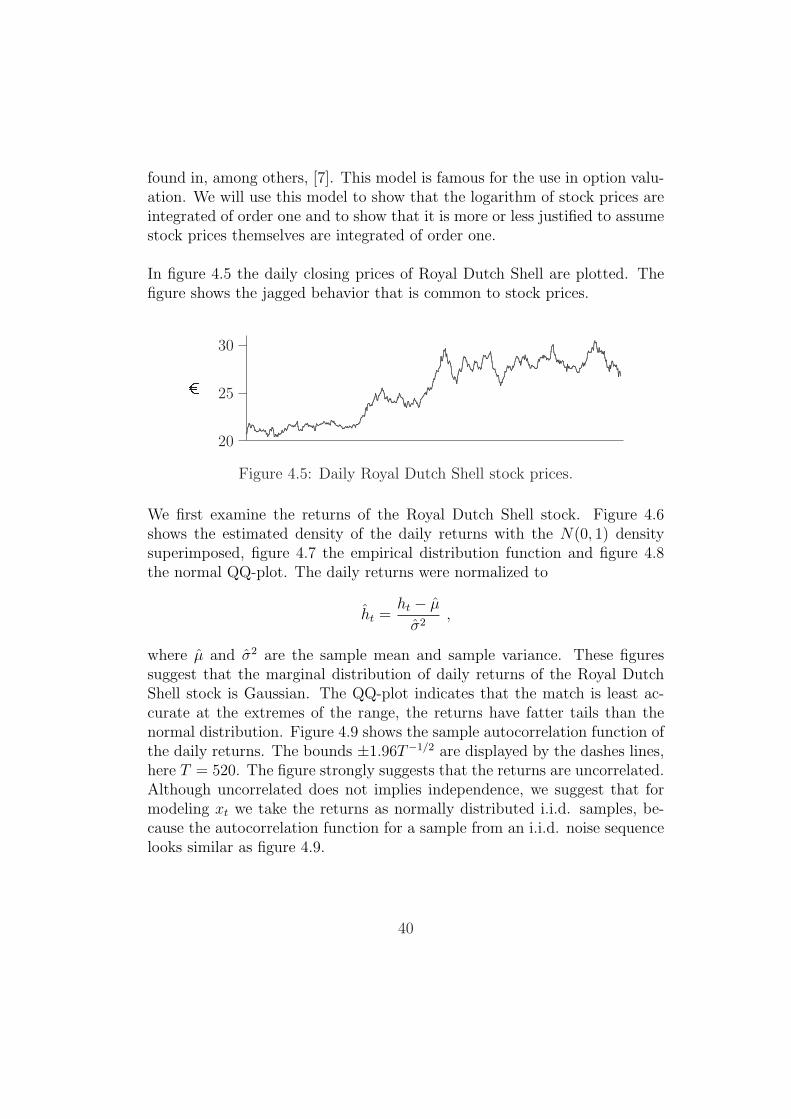
found in, among others, [7]. This model is famous for the use in option valu-ation. We will use this model to show that the logarithm of stock prices areintegrated of order one and to show that it is more or less justified to assumestock prices themselves are integrated of order one.

In figure 4.5 the daily closing prices of Royal Dutch Shell are plotted. Thefigure shows the jagged behavior that is common to stock prices.

20

25

30

¿

....................................................................................................................

.........................................................................

.................................................................

....................................................................................................

...........................................................

..................................................................................................................................................................................................................................................................................................................................................

.....................................................................

..............................................................................................................................................................................................................................................................................................................................................................................

...................................................................................................................

......................................................

................................................................................................................................................

.................................................................................................................................................................................................................................

..........................................................................

.........

........

......................................................................................................................................................................................

.........................................................................................................................................................................................................................................

.....................................................................................

............

Figure 4.5: Daily Royal Dutch Shell stock prices.

We first examine the returns of the Royal Dutch Shell stock. Figure 4.6shows the estimated density of the daily returns with the N(0, 1) densitysuperimposed, figure 4.7 the empirical distribution function and figure 4.8the normal QQ-plot. The daily returns were normalized to

ht =ht − µ

σ2,

where µ and σ2 are the sample mean and sample variance. These figuressuggest that the marginal distribution of daily returns of the Royal DutchShell stock is Gaussian. The QQ-plot indicates that the match is least ac-curate at the extremes of the range, the returns have fatter tails than thenormal distribution. Figure 4.9 shows the sample autocorrelation function ofthe daily returns. The bounds ±1.96T−1/2 are displayed by the dashes lines,here T = 520. The figure strongly suggests that the returns are uncorrelated.Although uncorrelated does not implies independence, we suggest that formodeling xt we take the returns as normally distributed i.i.d. samples, be-cause the autocorrelation function for a sample from an i.i.d. noise sequencelooks similar as figure 4.9.

40

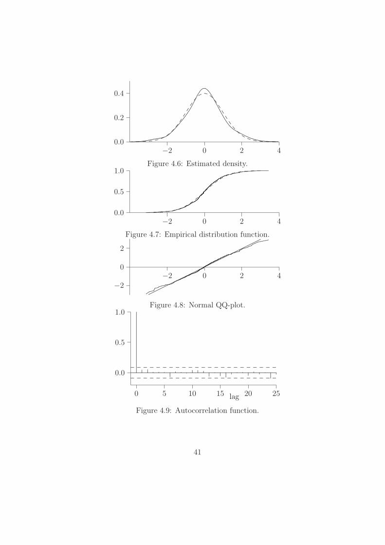
−2 0 2 40.0

0.2

0.4

...............................................................................................................................................

.......................................................................................................................................................................................................................................................................................................................................................................................................................................................................................................................................................................................................................................................................................................................................... ............. ............. ............. ............. .............

.....................................................................................................................

............. ..........................

..........................

..........................

..........................

............. ............. ............. ............. ............. ............. .

Figure 4.6: Estimated density.

−2 0 2 40.0

0.5

1.0

......................................................................................................................................................................................

....................................................................................................

....................................................................................................

....................................................................................................................................................................................................................................................................................................................................................................................................................................................................................................................

....................................................................................................

............................................................................................................................

.................................................................................................................................

............. ............. ............. ............. ............. ..........................

..........................

....................................................

..........................

............. ............. ............. ............. .............

Figure 4.7: Empirical distribution function.

−2 0 2 4

−2

0

2

......................................

..............................................

...................................................................................................

................................................................................................

..........................................................................................................................................

..........................................................................................................................................................................

..............................................................................................................................................................................

....................................................................................................................................................

...............................................................................................................

.........................................................................................

...................................................

.......................................

......................................................

..................................

..................................

.....................................

....................................

....................................

...................................

...................................

..................................

...................................

.....................................

....................................

....................................

..................................

...........................

Figure 4.8: Normal QQ-plot.

0 5 10 15 20 25

0.0

0.5

1.0

........

........

........

........

........

........

........

........

........

........

........

........

........

........

........

........

........

........

........

........

........

........

........

........

........

........

........

........

........

...

........

................

... ... .. ..................... .. .. ........

............

....... ................ .............

........................ .. .. ...........

.... ...... .. ......................

..........................................................................................................................................................................................................................................................................................................................................................................................................................................................................................................................................................................................

............. ............. ............. ............. ............. ............. ............. ............. ............. ............. ............. ............. ............. ............. ............. ............. ............. ............. ............. ............. ............. ............. .............

............. ............. ............. ............. ............. ............. ............. ............. ............. ............. ............. ............. ............. ............. ............. ............. ............. ............. ............. ............. ............. ............. .............

lag

Figure 4.9: Autocorrelation function.

41

Given the stock price x(0) = x0 at time t = 0, we like to come up witha process that describes the stock price x(t) for all times 0 ≤ t ≤ T . Asa starting point for the model we note that the value of a risk-free invest-ment D, like putting money on a savings account, changes over a small timeinterval δ as

D(t + δ) = D(t) + µδD(t),

where µ is the interest rate.

There is something that is called the efficient market hypothesis that saysthat the current stock price reflects all the information known to investors,and so any change in the price is due to new information. We may build thisinto our model by adding a random fluctuation to the interest rate equation.Let t = iδ, the discrete-time model becomes:

x(ti) = x(ti−1) + µ δ x(ti−1) + σ√

δ ui x(ti−1) , (4.1)

where the parameter µ > 0 represents an annual upward drift of the stockprices. The parameter σ ≥ 0 is a constant that determines the strength ofthe random fluctuations and is called the volatility. The random fluctuationsu1, u2, . . . are i.i.d N(0, 1). Notice that the returns [x(ti) − x(ti−1)]/x(ti−1)indeed form a normal i.i.d sequence.

We consider the time interval [0, t] with t = Lδ. Assume we know x(0) = x0,the discrete model (4.1) gives us expressions for x(δ), x(2δ), . . . , x(t). To de-rive a continuous model for the stock price, we let δ → 0 to get a limitingexpression for x(t).

The discrete model says that over each time δ the stock price gets multi-plied by a factor 1 + µ + σ

√δui, hence

x(t) = x0

L∏i=1

(1 + µδ + σ√

δui).

Dividing by x0 and taking logarithms gives

log

(x(t)

x0

)=

L∑i=1

log(1 + µδ + σ√

δui).

42

We are interested in the limit δ → 0, we exploit the approximationlog(1 + ε) ≈ ε− ε2/2 + · · · for small ε.

log

(x(t)

x0

)≈

L−1∑i=0

µδ + σ√

δui − 1

2σ2δu2

i .

This is justifiable because E(u2i ) is finite. We have ignored terms that involve

the power of δ3/2 or higher.

The expectation and the variance are:

E(µδ + σ√

δ − 1

2σ2δu2

i ) = µδ − 1

2σ2δ ,

var(µδ + σ√

δui − 1

2σ2δu2

i ) = σ2δ + higher powers of δ .

The Central Limit Theorem, which can be found in section 5.1, suggest thatlog(x(t)/x0) behaves like a normal random variable:

log

(x(t)

x0

)∼ N

((µ− 1

2σ2)t, σ2t

).

The limiting continuous-time expression for the stock price at fixed time tbecomes:

x(t) = x0e(µ− 1

2σ2)t+σ

√tW , where W ∼ N(0, 1).

For non-overlapping time intervals, the normal random variables that de-scribe the changes will be independent. We can describe the evolution of thestock over any sequence of time points 0 = t0 < t1 < t2 < · · · < tm by

x(ti) = x(ti−1)e(µ− 1

2σ2)(ti−ti−1)+σ

√ti−ti−1 Wi . (4.2)

This model guarantees that the stock prices is always positive, if x0 > 0.Model (4.2) is used a lot and is often referred to as geometric Brownian mo-tion.

We like to model the daily closing prices, we assume that the time inter-vals ti − ti−1 are equally spaced. That is, we set the time between Friday

43

evening and Monday evening equal to the time between Thursday eveningand Friday evening. We can write (4.2) as

xt = xt−1e(µ− 1

2σ2)δ+σ

√δ ut , (4.3)

with δ equal to 1/260, because there are approximately 260 trading days ina year. This is basically the same as the discrete model (4.1).

From this model follows that log xt is integrated of order one, because

log xt = log xt−1 + (µ− 1

2σ2)δ + σ

√δ ut,

hence

log xt − log xt−1 = (µ− 1

2σ2)δ + σ

√δ ut

= constant + Gaussian white noise.

This difference process of log xt is I(0) and because the process log xt itselfis not, it follows that log xt is I(1). This is one of the reasons why cointegra-tion tests are also applied to the logarithms of stock prices. Unfortunately,translating cointegration between the logarithm of two stocks into a trad-ing strategy is less intuitively clear then translating cointegration betweentwo stock prices themselves. When there is cointegration between the stockprices, trading the pair is very obvious. Let yt = (xt, yt) be two stock pricesprocesses which are cointegrated with cointegrating vector a. We ’normalize’this vector to (−α, 1), so yt − αxt is a stationary process with mean zero,which means that yt is approximately αxt. It could be that there is a con-stant in the cointegrating relation, than yt − αxt does not have mean zero.This will be discussed in the next section, for now we assume that the meanis zero. We treat yt−αxt as our spread process described in chapter 2, so wetrade pair (x, y) in the constant ratio α : 1. This is exactly the same as thetrading strategy, if we do not use the average ratio to calculate the spreadbut the least squares estimator.

If the logarithms of the stock prices xt and yt are cointegrated with coin-tegrating vector b, we normalize this to (−β, 1), then log yt − β log xt is astationary process. So log yt is approximately β log xt, we cannot trade log-arithms of stocks so we like to know the relation between xt and yt.

44

Let εt denote the residual process:

log yt − β log xt = εt.

The relation between xt and yt becomes:

yt = xβt eεt .

It is not clear how we can trade this relation, not with the strategy fromchapter 2. This is the reason why we want to test for cointegration on thestock prices and not on their logarithms, in order to do that we need xt and yt

to be integrated of order one. In chapter 9 we will make an attempt to comeup with a trading strategy if we have cointegration between the logarithmsof the stock prices.

Model (4.3) does not imply that xt is I(1), this is more easily seen in (4.1).The difference is

xt − xt−1 = µδxt−1 + σ√

δutxt−1,

this has not got a constant expectation, so according the derived stock pricemodel the difference process is not I(0). Fortunately, we look at the stockprices xT

t=0 for fixed T , µ is a small number between 0.01 and 0.1 andtypical values of σ are between 0.05 and 0.5, so it is not likely that xt−1

becomes very large or very small. That is why the differences divided by themean value of xt−1 look a lot like the returns:

xt − xt−1

xt−1

≈ xt − xt−1

xt−1

.

The returns are I(0), this indicates that the difference process ∆xt are alsomore or less I(0) and stock price process xt more or less I(1). We considera realization of model (4.3), where we take µ = 0.03, σ = 0.18 and x0 = 20shown in figure 4.10. The differences of this realizations is shown in figure4.11, which looks like pretty stationary. This indicates that realizations ofmodel (4.3) behave like they are I(1), while strictly under the model theyare not.

45

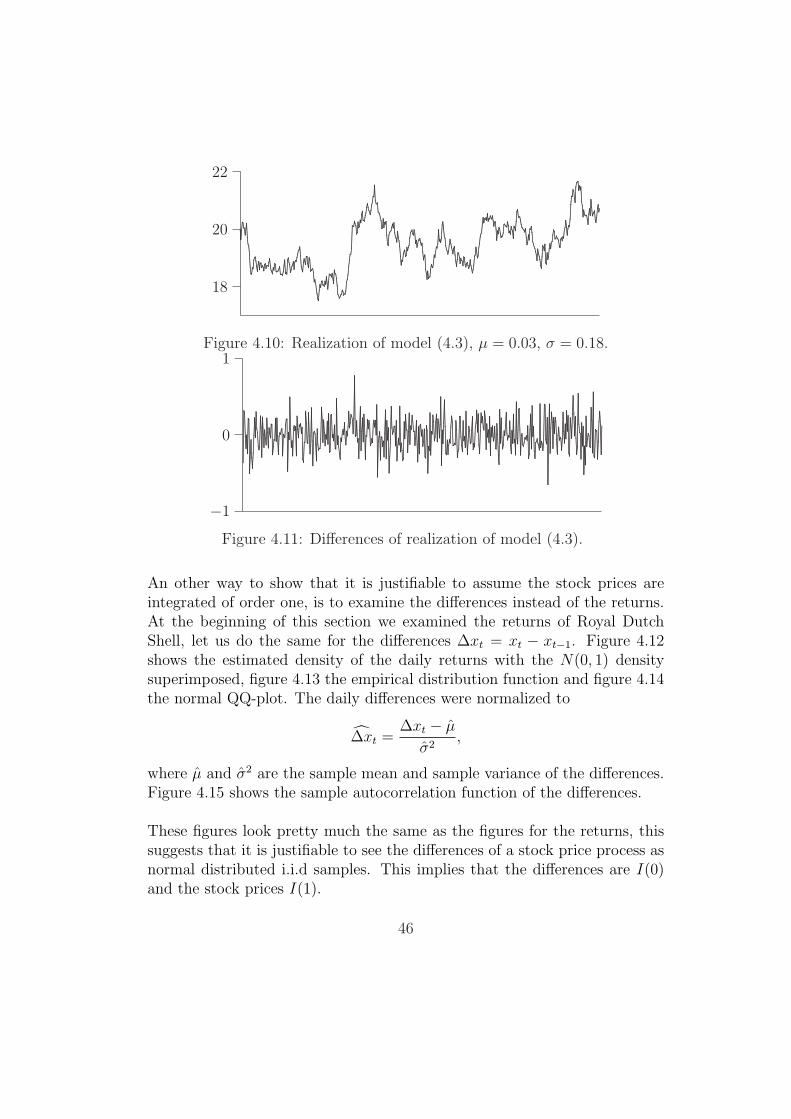
18

20

22

...............................................................................................................................................................................................................................................................................................................................................................................................................................................................................................................................................................................................................................................................................................................................................................................................................................................................................................................................................................................................................................................

........

.........

......................................................................................................................................................................................................................................................................

.......

.........................................................................................................................................................................................................................................................................................................................................................................................................................................................................................................................................

........

..............................................................................................................................................................................................................................................................................................................................................................................................................................................................................................................................................................................................................................................................................................................................................................................................................................................................................................................................................

........

.........

..............................................................................................................................................................................................................................................................................................................................................................................................................................................................................................................................................................................................................................................................................................................................................................................................................................................................................................................................................................................................

........

............................................................................................................................................................................................................................................................................................................................................................................................................................................................................

........

.............................................................................................................................................................................................................................................................................................................................................................................................................................................................................................................................................................................................................................

Figure 4.10: Realization of model (4.3), µ = 0.03, σ = 0.18.

−1

0

1

........

........

........

........

........

........

........

........

........

........

........

........

........................................................................................................................................................................................................................................................................................................................................................................................................................................................................................................................................................................................................................................................................................................................................................................................................................................................................................................................................................................................................................................................................................................................................................................................................................................................................................................................................................................................................................................................................................................................................................................................................................................................................................................................................................................................................................................................................................................................................................................................................................................................................................................................................................................................................................................................................................................................................................................................................................................................................................................................................................................................................................................................................................................................................................................................................................................................................................................................................................................................................................................................................................................................................................................................................................................................................................................................................................................................................................................................................................................................................................................................................................................................................................................................................................................................................................................................................................................................................................................................................................................................................................................................................................................................................................................................................................................................................................................................................................................................................................................................................................................................................................................................................................................................................................................................................................................................................................................................................................................................................................................................................................................................................................................................................................................................................................................................................................................................................................................................................................................................................................................................................................................................................................................................................................................................................................................................................................................................................................................................................................................................................................................................................................................................................................................................................................................................................................................................................................................................................................................................................................................................................................................................................................................................................................................................................................................................................................................................................................................................................................................................................................................................................................................................................................................................................................................................................................................................................................................................................................................................................................................................................................................................................................................................................................................................................................................................................................................................................................................................................................................................................................................................................................................................................................................................................................................................................................................................................................................................................................................................................................................................................................................................................................................................................................................................................................................................................................................................................................................................................................................................................................................................................................................................................................................................................................................................................................................................................................................................................................................................................................................................................................................................................................................................................................................................................................................................................................................................................................................................................................................................................................................................................................................................................................................................................................................................................................................................................................................................................................................................................................................................................................................................................................................................................................................................................................................................................................................................................................................................................................................................................................................................................................................................................................................................................................................................................................................................................................................................................................................................................................................................................................................................................................................................................................................................................................................................................................................................................................................................................................................................................................................................................................................................................................................................................................................................................................................................................................................................................................................................................................................................................................................................................................................................................................................................................................................................................................................................................................................................................................................................................................................................................................................................................................................................................................................................................................................................................................................................................................................................................................................................................................................................................................................................................................................................................................................................................................................................................................................................................................................................................................................................................................................................................................................................................................................................................................................................................................................................................................................................................................................................................................................................................................................................................................................................................................................................................................................................................................................................................................................................................................................................................................................................................................................................................................................................................................................................................................................................................................................................................................................................................................................................................................................................................................................................................................................................................................................................................................................................................................................................................................................................................................................................................................................................................................................................................................................................................................................................................................................................................................................................................................................................................................................................................................................................................................................................................................................................................................................................................................................................................................................................................................

Figure 4.11: Differences of realization of model (4.3).

An other way to show that it is justifiable to assume the stock prices areintegrated of order one, is to examine the differences instead of the returns.At the beginning of this section we examined the returns of Royal DutchShell, let us do the same for the differences ∆xt = xt − xt−1. Figure 4.12shows the estimated density of the daily returns with the N(0, 1) densitysuperimposed, figure 4.13 the empirical distribution function and figure 4.14the normal QQ-plot. The daily differences were normalized to

∆xt =∆xt − µ

σ2,

where µ and σ2 are the sample mean and sample variance of the differences.Figure 4.15 shows the sample autocorrelation function of the differences.

These figures look pretty much the same as the figures for the returns, thissuggests that it is justifiable to see the differences of a stock price process asnormal distributed i.i.d samples. This implies that the differences are I(0)and the stock prices I(1).

46

−2 0 2 40.0

0.2

0.4

....................................................................................................................

......................................................................................................................................................................................................................................................................................................................................................................................................................................................................................................................................................................................................................................................................................................................................... ............. ............. ............. ............. .............

.....................................................................................................................

............. ..........................

..........................

..........................

..........................

............. ............. ............. ............. ............. ............. .

Figure 4.12: Estimated density.

−2 0 2 40.0

0.5

1.0

.......................................................................................................................................................................................

........................................................................................................

....................................................................................................

....................................................................................................................................................................................................................................................................................................................................................................................................................................................................................................................

.....................................................................................................

......................................................................................................................

......................................................................................................................................................

............. ............. ............. ............. ............. ..........................

..........................

....................................................

..........................

............. ............. ............. ............. .............

Figure 4.13: Empirical distribution function.

−2 0 2 4

−2

0

2

................................................

.................................................................................

................................................................

.....................................................................................................

..........................................................................................................................................

..........................................................................................................................................................................

..............................................................................................................................................................................

....................................................................................................................................................

.............................................................................................................

.................................................................................

........................................................

..........................................

......................................................................

..................................

..................................

.....................................

....................................

....................................

...................................

...................................

..................................

...................................

.....................................

....................................

....................................

..................................

...........................

Figure 4.14: Normal QQ-plot.

0 5 10 15 20 25

0.0

0.5

1.0

........

........

........

........

........

........

........

........

........

........

........

........

........

........

........

........

........

........

........

........

........

........

........

........

........

........

........

........

........

...

........

.....................

...... .. .. ................. ... ..... ........

............

...... ................ ............

....................

............. ... ...........

.. .......... ......................

............................................................................................................................................................................................................................................................................................................................................................................................................................................................................................................................................................................................

............. ............. ............. ............. ............. ............. ............. ............. ............. ............. ............. ............. ............. ............. ............. ............. ............. ............. ............. ............. ............. ............. .............

............. ............. ............. ............. ............. ............. ............. ............. ............. ............. ............. ............. ............. ............. ............. ............. ............. ............. ............. ............. ............. ............. .............

lag

Figure 4.15: Autocorrelation function.

47

So far we have discussed why it is likely that stock price processes are in-tegrated of order one, but we can also do unit root tests on the data wewant to test for cointegration. The unit root test we use in this report is the(Augmented) Dickey-Fuller test, introduced in chapter 3. The first test is:

H0 : xt ∼ I(1) against H1 : xt ∼ I(0).

The outcome should be to not reject H0. The second test is:

H0 : xt ∼ I(2) against H1 : xt ∼ I(1),

which is equivalent to:

H0 : ∆xt ∼ I(1) against H1 : ∆xt ∼ I(0).

The outcome of this second test should be to reject H0, which makes is likelythat the price processes are I(1). Which case of the DF-test should be usedis discussed in the next section, the critical values of these tests are derivedin chapter 5 and the results of these tests for data used in this report arestated in chapter 7.

4.3 Engle-Granger method

The question remains how to test for cointegration. There are several meth-ods for testing for cointegration. R.F. Engle and C.W.J. Granger were thefirst to develop the key concepts of cointegration, which can be found in [5].They received the nobel prize in economics in 2003 for their work on cointe-gration and ARCH models. The approach of testing for cointegration will beto test the null hypothesis that there is no cointegration among the elementsof an (n × 1) vector yt. Rejection of the null hypothesis is then taken asevidence of cointegration.

The Engle-Granger test is a two-step process, which should be preceded byexamining if each component of yt is I(1) which was discussed in the previoussection. Let us assume that this condition is fulfilled. A vector process yt iscointegrated if there exists a linear combination of its components a′yt thatis stationary. The first step in the Engle-Granger test is to estimate a, this isdone with an OLS (Ordinary Least Squares) regression. The second step is

48

to test whether the residuals of the regression are stationary using a Dickey-Fuller test. Because if the residuals are stationary, the linear combinationa′yt is stationary, which means yt is cointegrated with cointegrating vector a.

Looking from a pairs trading point of view we have two stock prices pro-cesses, yt = (xt, yt). We like xt and yt to be cointegrated such that thespread εt = yt − αxt oscillates around zero, again we have ’normalized’ thecointegrating vector a to (−α, 1). A stationary process has constant expecta-tion but it is not necessarily equal to zero. In order to get a stationary processwith mean zero, we can include a constant in the cointegration relation suchthat the spread becomes:

εt = yt − αxt − α0.

For example, consider the pair (xt, yt) which is generated with the relation:

yt = 2xt + 20 + εt,

so α = 2 and α0 = 20. Figure 4.16 shows xt and yt.

0

50

100

150

..............................................................................................................

............................................................................................................................

..............................................................................

.......................................................................................................................................................................................................................................................................................

........................................................................

.......................................................................................................................................................................................................................................................................................................................................................

............................................................................................................

.....................................................................................................

.....................................................................

..................................................................

.................................................................................................................................................

.............................................................................................................................

.............................................................................................................

.............................................................................................................................................................................................................

...........................................................................................................................................

.....................................................................................................................................................................................................................................................................................................................................................................

.........................................................................

................................................................................

Figure 4.16: Paths xt and yt for α0 = 20.

Normally we do not know the exact value of α and α0, so we have to estimatethem. According to the Engle-Granger method we do this with OLS. We havetwo possibilities, regression with and without intercept. In the first situation,regression with intercept, we get

αα0 = 2.01 α0 = 19.67.

In the second, regression without intercept:

α¬α0 = 2.41.

49

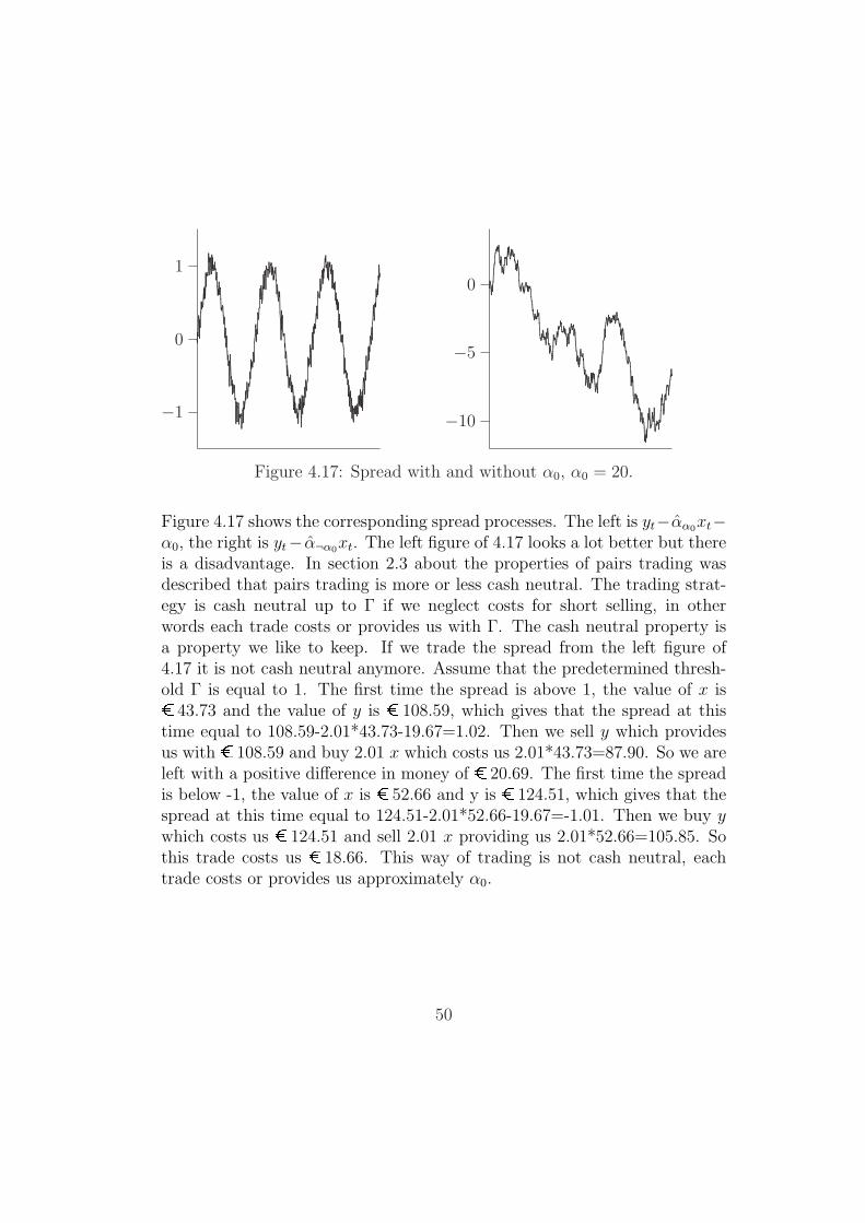
−1

0

1

...............

........

.................

........

........

.........

................................................................................................................................................................................................................................................................................................................................................................................................................................................................................................................................................................................................................................................................................................................................................................................................................................................................................................................................................................................................................................................................................................................................................................................................................................................................................................................................................................................................................................................................................................................................................................................................................................................................................................................................................................................................................................................................................................................................................................................................................................................................................................................................................................................................................................................................................................................................................................................................................................................................................................................................................................................................................................................................................................................................................................................................................................................................................................................................................................................................................................................................................................................................................................................................................................................................................................................................................................................................................................................................................................................................................................................................................................................................................................................................................................................................................................................................................................................................................................................................................................................................................................................................................................................................................................................................................................................................................................................................................................................................................................................................................................................................................................................................................................................................................................................................................................................................................................................................................................................................................................................................................................................................................................................................................................................................................................................................................................................................................................................................................................................................................................................................................................................................................................................................................................................................................................................................................................................................................................................................................................................................................................................................................................................................................................................................................................................................................................................................................................................................................................................................................................................................................................................................................................................................................................................................................................................................................................................................................................................................................................................................................................................................................................

−10

−5

0 ....................................................................................................................................................................................................................................................................................................................................................................................................................................................................................................................................................................................................................................................................................................................................................................................................................................................................................................................................................................................................................................................................................................................................................................................................................................................................................................................................................................................................................................................................................................................................................................................................................................................................................................................................................................................................................................................................................................................................................................................................................................................................................................................................................................................................................................................................................................................................................................................................................................................................................................................................................................................................................................................................................................................................................................................................................................................................................................................................................................................................................................................................................................................................................................................................................................................................................................................................................................................................................................................................................................................................................................................................................................................................................................................................................

Figure 4.17: Spread with and without α0, α0 = 20.

Figure 4.17 shows the corresponding spread processes. The left is yt−αα0xt−α0, the right is yt− α¬α0xt. The left figure of 4.17 looks a lot better but thereis a disadvantage. In section 2.3 about the properties of pairs trading wasdescribed that pairs trading is more or less cash neutral. The trading strat-egy is cash neutral up to Γ if we neglect costs for short selling, in otherwords each trade costs or provides us with Γ. The cash neutral property isa property we like to keep. If we trade the spread from the left figure of4.17 it is not cash neutral anymore. Assume that the predetermined thresh-old Γ is equal to 1. The first time the spread is above 1, the value of x is¿ 43.73 and the value of y is ¿ 108.59, which gives that the spread at thistime equal to 108.59-2.01*43.73-19.67=1.02. Then we sell y which providesus with ¿ 108.59 and buy 2.01 x which costs us 2.01*43.73=87.90. So we areleft with a positive difference in money of ¿ 20.69. The first time the spreadis below -1, the value of x is ¿ 52.66 and y is ¿ 124.51, which gives that thespread at this time equal to 124.51-2.01*52.66-19.67=-1.01. Then we buy ywhich costs us ¿ 124.51 and sell 2.01 x providing us 2.01*52.66=105.85. Sothis trade costs us ¿ 18.66. This way of trading is not cash neutral, eachtrade costs or provides us approximately α0.

50

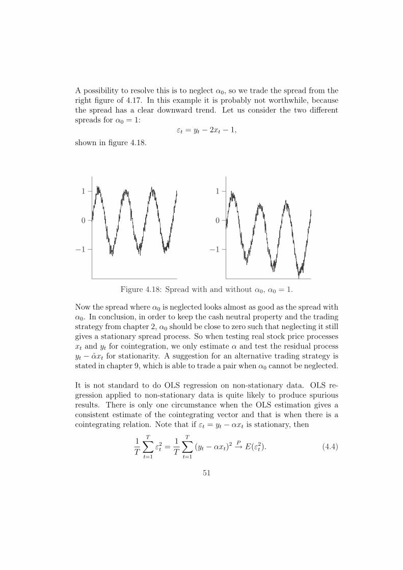
A possibility to resolve this is to neglect α0, so we trade the spread from theright figure of 4.17. In this example it is probably not worthwhile, becausethe spread has a clear downward trend. Let us consider the two differentspreads for α0 = 1:

εt = yt − 2xt − 1,

shown in figure 4.18.

−1

0

1

..............

....................

........

.........

.....................................................................................................................................................................................................................................................................................................................................................................................................................................................................................................................................................................................................................................................................................................................................................................................................................................................................................................................................................................................................................................................................................................................................................................................................................................................................................................................................................................................................................................................................................................................................................................................................................................................................................................................................................................................................................................................................................................................................................................................................................................................................................................................................................................................................................................................................................................................................................................................................................................................................................................................................................................................................................................................................................................................................................................................................................................................................................................................................................................................................................................................................................................................................................................................................................................................................................................................................................................................................................................................................................................................................................................................................................................................................................................................................................................................................................................................................................................................................................................................................................................................................................................................................................................................................................................................................................................................................................................................................................................................................................................................................................................................................................................................................................................................................................................................................................................................................................................................................................................................................................................................................................................................................................................................................................................................................................................................................................................................................................................................................................................................................................................................................................................................................................................................................................................................................................................................................................................................................................................................................................................................................................................................................................................................................................

−1

0

1

..............

........

..................

........

.........

............................................................................................................................................................................................................................................................................................................................................................................................................................................................................................................................................................................................................................................................................................................................................................................................................................................................................................................................................................................................................................................................................................................................................................................................................................................................................................................................................................................................................................................................................................................................................................................................................................................................................................................................................................................................................................................................................................................................................................................................................................................................................................................................................................................................................................................................................................................................................................................................................................................................................................................................................................................................................................................................................................................................................................................................................................................................................................................................................................................................................................................................................................................................................................................................................................................................................................................................................................................................................................................................................................................................................................................................................................................................................................................................................................................................................................................................................................................................................................................................................................................................................................................................................................................................................................................................................................................................................................................................................................................................................................................................................................................................................................................................................................................................................................................................................................................................................................................................................................................................................................................................................................................................................................................................................................................................................................................................................................................................................................................................................................................................................................................................................................................................................................................................................................................................................................................................................................................................................................................................................................................................................................................................................................................................................................................................................................

Figure 4.18: Spread with and without α0, α0 = 1.

Now the spread where α0 is neglected looks almost as good as the spread withα0. In conclusion, in order to keep the cash neutral property and the tradingstrategy from chapter 2, α0 should be close to zero such that neglecting it stillgives a stationary spread process. So when testing real stock price processesxt and yt for cointegration, we only estimate α and test the residual processyt − αxt for stationarity. A suggestion for an alternative trading strategy isstated in chapter 9, which is able to trade a pair when α0 cannot be neglected.

It is not standard to do OLS regression on non-stationary data. OLS re-gression applied to non-stationary data is quite likely to produce spuriousresults. There is only one circumstance when the OLS estimation gives aconsistent estimate of the cointegrating vector and that is when there is acointegrating relation. Note that if εt = yt − αxt is stationary, then

1

T

T∑t=1

ε2t =

1

T

T∑t=1

(yt − αxt)2 P→ E(ε2

t ). (4.4)

51

By contrast, if (−1, α) is not a cointegrating vector between x and y, thenyt − αxt is I(1) and from proposition 2 in section 5.6,

1

T 2

T∑t=1

(yt − αxt)2 D→ λ2

∫ 1

0

W (r)2 dr,

where W (r) is standard Brownian motion which will be defined in chapter5 and λ is a parameter determined by the autocovariances of ∆εt. Hence,if (−1, α) is not a cointegrating vector, the statistic in (4.4) would divergeto +∞. This suggests that we can obtain a consistent estimate of a cointe-grating vector by choosing α so as to minimize (4.4). It turns out that theOLS estimator for α, also when α0 is included in the regression, converges atrate T . This is analyzed by Philips and Durlauf in [12].

Now that we have a method for estimating the cointegrating vector, thesecond step in the Engle-Granger method is examining the residuals with aDickey-Fuller test. In chapter 3 was described that there are several cases,so the question remains which case do we use when testing for cointegration.In most literature about cointegration, it is not stated which case is used andwhy, but from the critical values used can be seen that case 2 is used mostoften. One discussion found in Hamilton [6], is the following:

Which case is the ’correct’ case to use to test the null hypothesisof a unit root? The answer depends on why we are interested intesting for a unit root. If the analyst has a specific null hypothe-sis about the process that generated the data, then obviously thiswould guide the choice of test. In the absence of such guidance,one general principal would be to fit a specification that is a plausi-ble description of the data under both the null and the alternative.This principle would suggest using case 4 for a series with a obvi-ous trend and the case 2 for series without a significant trend. Forexample, the nominal interest rate series used in the examples inthis section. There is no economic theory to suggest that nominalinterest rates should exhibit a deterministic time trend, and so anatural null hypothesis is that the true process is a random walkwithout trend. In terms of framing a plausible alternative, it isdifficult to maintain that these data could have been generated byit = ρit−1 +ut with |ρ| significantly less than 1. If these data were

52

to be described by a stationary process, surely the process wouldhave a positive mean. This argues for including a constant termin the estimated regression, even though under the null hypothesisthe true process does not contain a constant term. Thus, case 2is a sensible approach for these data.

We do not have a specific null hypothesis, so according to this quote weshould use case 2 because there is no trend in spread processes. In the nextchapter we investigate the power of the three different tests, case 1 throughcase 3, maybe we can find another reason to use Dickey-Fuller case 2.

So far we have looked at cointegration between two stocks because of pairstrading. However, pairs trading with three of more stocks in a ’pair’ is veryinteresting. Cointegration is defined for a (n× 1) vector yt and the tradingstrategy is easily extended for three or more stocks. For example, consider apair of three stocks yt = (xt, yt, zt) who are cointegrated with cointegratingvector (−α1,−α2, 1). Then we calculate the spread as

st = zt − α1xt − α2yt,

which we trade the same way as before. When the spread reaches Γ we sell1 z and buy α1 times x and α2 times y. When the spread goes below −Γ wereverse our position and lock in a profit of at least 2Γ. The threshold Γ isdetermined in the same way as in chapter 2, we just try a few on historicaldata and take the best one.

If the number of stocks in a pair is greater than two, n > 2, the Engle-Grangermethod has a disadvantage. We estimate the cointegrating vector with OLSregression, if yt = (y1t, y2t, . . . , ynt) we regress y1t on (y2t, y3t, . . . , ynt). So thefirst element of the cointegrating vector is set to be unity. This normalizationis not harmless if the first variable y1t does not appear in the cointegratingrelation at all, in other words, its coefficients is equal to zero but is set to one.

A second disadvantage, which exist also when n = 2, is that the methodis not symmetric. Suppose n = 2, we regress y1t on y2t:

y1t = αy2t + ut.

We might equally well have normalized the coefficient of y2t, so the regressionwould be

y2t = βy1t + vt.

53

Then the OLS estimate β is not simply the inverse of α, meaning that thesetwo regression will give different estimates of the cointegrating vector. Thus,choosing which variable to call y1 and which to call y2 might end up makinga difference for the evidence one finds for cointegration.

For these reasons we discuss the Johansen method in the next section. Firsta summary is given for testing on cointegration with the Engle-Grangermethod:

Given is (n× 1) vector yt = (y1t, y2t, . . . , ynt).

Examine or assume that each individual variable yit is I(1).

Then yt is cointegrated if a′yt is I(0) for some nonzero vector a.

Regress y1t on (y2t, . . . , ynt), a constant maybe included but with ourtrading strategy we do not want to include this constant. This regres-sion gives the estimation a.

Then the residuals of this regression, which is our spread process, aregiven by

e = y1t − a2y2t − · · · − anynt,

which resembles the real error process:

εt = y1t − a2y2t − · · · − anynt.

The Dickey-Fuller test assumes that εt follows an AR(p) model, withan unit root and with or without a constant term. If we use case 2,which is suggested by the above quote, we assume that the true modeldoes not have a constant but we include a constant in the estimatedmodel. So the Dickey-Fuller case 2 assumes the true model of εt is

εt = ρεt−1 + β1∆εt−1 + · · ·+ βp−1∆εt−p+1 + ηt,

with ρ = 1.

To estimate p we fit an AR(k) model with OLS on et for k = 1, . . . , K.The value of k with the smallest information criteria AIC(k), BIC(k)and HIC(k) is the estimate for the model order p. If the informationcriteria give different values, we take the rounded mean.

54

We use the AR(p) fit

et = c + ρet−1 + β1∆et−1 + · · ·+ βp−1∆et−p+1 + nt ,

to calculate the Dickey-Fuller test statistic

ρ− 1

σρ

,

where ρ is the OLS estimate of ρ and σρ is the standard error for theestimated coefficient.

Compare the outcome with the critical values of the Dickey-Fuller test.

The critical values of the Dickey-Fuller test will be derived and simulated inthe next chapter. Engle-Granger is a two-step method, first we do an OLSregression and then a Dickey-Fuller test. In chapter 6 we will examine if thefirst step influences the critical values, in other words, are the critical valuesfor Engle-Granger really the same as for Dickey-Fuller.

4.4 Johansen method

The Johansen method also known as ’full-information maximum likelihood’was developed by Søren Johansen in [8] and [9]. This method allows us to testfor the number of cointegrating relations. An (n× 1) vector yt has h cointe-grating relations if there exists h linearly independent vectors a1, a2, . . . , ah

such that a′iyt is stationary. If such vectors exist, their values are not unique,since any linear combination of a1, a2, . . . , ah is also a cointegrating vector.With the Engle-Granger method this was resolved by setting the first ele-ment in the cointegrating vector equal to one. As mentioned before this hassome disadvantages. In this section the Johansen method is summarized, noproof or argumentation is given. These can be found in [8] and [9].

Let yt be an (n × 1) vector. The Johansen method assumes that yt fol-lows a VAR(p) model

yt = c + Φ1yt−1 + · · ·+ Φpyt−p + εt, (4.5)

where c is an (n× 1) vector and Φi is an (n× n) matrix.

55

Model (4.5) can be written as

yt = c + ρyt−1 + β1∆yt−1 + · · ·+ βp−1∆yt−p+1 + εt, (4.6)

where

ρ = Φ1 + Φ2 + · · ·+ Φp ,

βi = − (Φi+1 + Φi+2 + · · ·+ Φp) , for i = 1, 2, . . . , p− 1.

Subtracting yt−1 from both sides of (4.6) results in

∆yt = c + β0yt−1 + β1∆yt−1 + · · ·+ βp−1∆yt−p+1 + εt, (4.7)

with

E(εt) = 0,

E(εtετ ) =

Ω for t = τ,0 otherwise.

Johansen showed that under the null hypothesis of h cointegrating relations,only h separate linear combinations of yt appear in (4.7). This implies thatβ0 can be written in the form

β0 = −BA′ , (4.8)

for B an (n× h) matrix and A′ an (h× n) matrix.

If we consider a sample of T +p observations, denoted (y−p+1,y−p+2, . . . ,yT ),and if the errors εt are Gaussian, the log likelihood of (y1,y2, . . . ,yT ) con-ditional on (y−p+1,y−p+2, . . . ,y0) is given by

L(Ω, c,β0,β1, . . . , βp−1) = (4.9)

−Tn

2log(2π)− T

2log |Ω|

−1

2

T∑t=1

[(∆yt − c− β0yt−1 − β1∆yt−1 − · · · − βp−1∆yt−p+1)

′

× Ω−1(∆yt − c− β0yt−1 − β1∆yt−1 − · · · − βp−1∆yt−p+1)].

56

The goal is to choose (Ω, c,β0,β1, . . . , βp−1) so as to maximize (4.9) subjectto the constraint that β can be written in the form of (4.8). The Johansenmethod calculates the maximum likelihood estimates of (Ω, c, β0,β1, . . . , βp−1).

The first step of the Johansen method is to estimate a VAR(p − 1) for∆yt. That is, regress ∆yit on a constant and all elements of the vectors∆yt−1, . . . , ∆yt−p+1 with OLS. Collect the i = 1, 2, . . . , n regressions in vec-tor form

∆yt = π0 + Π1∆yt−1 + · · ·+ Πp−1∆yt−p+1 + ut. (4.10)

We also estimate a second regression, we regress yt−1 on a constant and∆yt−1, . . . , ∆yt−p+1

yt−1 = θ + χ1∆yt−1 + · · ·+ χp−1∆yt−p+1 + vt. (4.11)

The second step is to calculate the sample covariance matrices of the OLSresiduals ut and vt:

Σvv =1

T

T∑t=1

vtv′t ,

Σuu =1

T

T∑t=1

utu′t ,

Σuv =1

T

T∑t=1

utv′t ,

Σvu = Σuv′ .

From these, find the eigenvalues of the matrix

Σ−1vvΣvuΣ

−1uuΣuv , (4.12)

with the eigenvalues ordered λ1 > λ2 > · · · > λn. The maximum valueattained by the log likelihood function subject to the constraint that thereare h cointegrating relations is given by

L∗0 = −Tn

2log(2π)− Tn

2− T

2log |Σuu| − T

2

h∑i=1

log(1− λi). (4.13)

57

The third step is to calculate the maximum likelihood estimates of the pa-rameters. Let a1, . . . , ah denote the (n× 1) eigenvectors of (4.12) associatedwith the h largest eigenvalues. These provide a basis for the space of coin-tegrating relations. That is, the maximum likelihood estimate is that anycointegrating vector can be written in the form

a = b1a1 + b2a2 + · · ·+ bhah ,

for some choice of scalers b1, . . . , bh. Johansen suggests normalizing thesevector ai such that a′iΣvvai = 1. Collect the first h normalized vectors in aan (n× h) matrix A:

A =[

a1 a2 · · · ah

].

Then the maximum likelihood estimate of β0 is given by

β0 = ΣuvAA′ .

The maximum likelihood estimate of c is

c = π0 − β0 .

Now we are ready for hypothesis testing. Under the null hypothesis that thereare exactly h cointegrating relations, the largest value that can be achievedfor the log likelihood function was given by (4.13). Consider the alternativehypothesis that there are n cointegrating relations. This means that everylinear combination of yt is stationary, in which case yt−1 would appear in(4.7) without constraints and no restrictions are imposed on β0. The valuefor the log likelihood function in the absence of constraints is given by

L∗1 = −Tn

2log(2π)− Tn

2− T

2log |Σuu| − T

2

n∑i=1

log(1− λi). (4.14)

A likelihood ratio test of

H0 : h relations against H1 : n relations,

can be based on

2(L∗1 − L∗0) = −T

n∑

i=h+1

log(1− λi). (4.15)

58

An other approach would be to test the null hypothesis of h cointegratingrelations against h + 1 cointegrating relations. A likelihood ratio test of

H0 : h relations against H1 : h + 1 relations,

can be based on

2(L∗1 − L∗0) = −T log(1− λh+1). (4.16)

Like with the Dickey-Fuller test, we need to distinguish several cases. Thereare also three cases for the Johansen method, but they are different than theDickey-Fuller cases:

Case 1 : The true value of the constant c in (4.7) is zero, meaning thatthere is no intercept in any of the cointegrating relations and no determin-istic time trend in any of the elements of yt. There is no constant termincluded in the regressions (4.10) and (4.11).

Case 2 : The true value of the constant c in (4.7) is such that there areno deterministic time trends in any of the elements of yt. There are no re-strictions on the constant term in the estimation of the regressions (4.10)and (4.11).

Case 3 : The true value of the constant c in (4.7) is such that one or moreelements of yt exhibit deterministic time trend. There are no restrictions onthe constant term in the estimation of the regressions (4.10) and (4.11).

For both tests, which can be based on (4.15) and (4.16), the critical val-ues for the three different cases can be found in [10] and [11]. Unfortunately,the critical values are for a sample size of T = 400. Although the data ofthe ten pairs IMC provided consist of 520 observations, these critical valueswill be used when testing the ten pairs for cointegration. I assume that thecritical values are not that different for a sample size of 520. For case 1 thisis very likely because Johansen showed that the asymptotic distribution oftest statistic (4.15) is the same as that of the trace of matrix

Q =

[∫ 1

0

W(r)dW(r)′]′ [∫ 1

0

W(r)W(r)′dr

]−1 [∫ 1

0

W(r)dW(r)′]

where W(r) is g-dimensional standard Brownian motion, with g = n− h.

59

And fortunately, case 1 is the case we will use because we do not wantan intercept in the cointegrating relations, as was explained in the previoussection, and we assume there is no deterministic time trend in the price pro-cesses. The Johansen case 1 test can be compared with the Dickey-Fullercase 1 test, there is no constant and we do not estimate one. There is notreally a Johansen case which can be compared to the Dickey-Fuller case 2,with the Johansen case 2 test, the constant c is not necessarily equal to zero.The critical values for case 1 and T = 400 for both test statistics (4.15) and(4.16) are shown in tables 4.1 and 4.2 respectively.

Table 4.1: Critical values for test statistic (4.15).Case 1

g 1% 5% 10%1 6.51 3.84 2.862 16.31 12.53 10.473 29.75 24.31 21.634 45.58 39.89 36.585 66.52 59.46 55.44

Table 4.2: Critical values for test statistic (4.16).Case 1

g 1% 5% 10%1 6.51 3.84 2.862 15.69 11.44 9.523 22.99 17.89 15.594 28.82 23.80 21.585 35.17 30.04 27.62

Note that if g = 1, then n = h + 1. In this case the two tests are iden-tical. For this reason the first rows of the tables are the same.

With two stocks in pair, we can do several hypothesis tests:

1) H0 : 0 relations against H1 : 2 relations,2) H0 : 0 relations against H1 : 1 relation,3) H0 : 1 relation against H1 : 2 relations.

60

For the first test, we use the second row of table 4.1. We basically test thenull of no cointegration between the two stocks against the stocks themselvesbeing stationary. Although the alternative hypothesis does not imply ’real’cointegration, because every linear combination of yt is stationary since yt isalready stationary, rejection of the null is taken as evidence of cointegration.

For the second test, we use the second row of table 4.2. We test the nullof no cointegration between the against the alternative of a single cointegra-tion relation.

For the third test, we use the first row of either table. We test the nullof one cointegrating relation against the stock prices being stationary al-ready. Basically we test if the relation is a ’real’ cointegrating relation.

If the third null hypothesis is rejected, the test indicates there are two coin-tegrating relations which means the stock prices themselves are stationary.As we saw in section 4.2 we do not think that stock prices are stationary,but if they are we can trade them as a pair like any other pair. We couldeven trade each stock as a spread process. That means, we apply the tradingstrategy on the price process instead of the spread process. But this wouldnot be cash and market neutral anymore, and is seen as far more risky. Sowith two stocks in a pair, we would like there to be one or two cointegratingrelations, but we expect there is only one. In chapter 7 the results of thedifferent tests for the 10 pairs are given. They are compared with the resultsfrom the Engle-Granger method.

In the previous section was stated that the Johansen method has an ad-vantage compared to the Engle-Granger method when there are more thantwo stocks in a pair, n > 2. With Johansen we do not impose the first el-ement of the cointegrating relation to be unity, we normalize the estimatedcointegrating relation such that the first element is unity or as Johansen pro-posed, normalizing such that a′iΣvvai = 1. With three stocks in a pair, wewould like there to be one, two or three cointegrating relations but we expectthat there are no more than two. With our pair trading strategy it does notmatter how many relations there are as long as the stock are cointegrated,because we only trade one relation. This relation will be the eigenvectorcorresponding to the largest eigenvalue of the matrix in (4.12) because, ac-cording to Hamilton [6], this results in the most stationary spread process.

61

4.5 Alternative method

In this section a start is made with an alternative method. Assume, like theEngle-Granger and Johansen method, price processes xt and yt are integratedof order one: xt, yt ∼ I(1). Denote with zt the vector of the differences ofthese price processes

zt =

(xt − xt−1

yt − yt−1

).

Then each component of zt is I(0), i.e. stationary. Notice that

(xt − x0

yt − y0

)=

t∑i=1

zi .

Two price processes are cointegrated if a linear combination of them is sta-tionary, i.e. constant mean, constant variance and autocovariances that donot depend on t. In this section we like to find out if zt can be representedas an VAR(p) or as a vector MA(q) process.

Engle and Granger showed that a cointegrated system can never be repre-sented by a finite-order vector autoregression in the differenced data ∆yt =zt. The outline of the deduction is that if zt is causal, i.e. zt can be writtenas a linear combination of past innovations, and (xt, yt) are cointegrated thenzt is non-invertible. This implies that if (xt, yt) are cointegrated zt cannotbe represented by a VAR(p).

If we assume zt to be an vector MA(q) process, we can find restrictionson the parameters of the model to ensure a linear combination of (xt, yt)such that it is stationary exists. Let us examine this for q = 2:

zt = Θ2wt−2 + Θ1wt−1 + Θ0wt ,

where wt is i.i.d N2(0, Σ) and Θ0 = I. Notice that a MA(q) process is alwaysstationary.

Thent∑

i=1

zi = Θ2w−1 + (Θ2 + Θ1)w0 + (Θ2 + Θ1 + Θ0)t−2∑i=1

wi

+ (Θ1 + Θ0)wt−1 + Θ0wt .

62

If v is a cointegrating vector, i.e. a vector such that v∑t

i=1 zi is stationary,than every multiple of v is also a cointegrating vector. We can make somekind of normalization so we can write v = [−α 1]. For t > 2

(yt − αxt) − (y0 − αx0) = [−α 1]∑t

i=1 zi

= [−α 1]Θ2w−1 + [−α 1](Θ2 + Θ1)w0 (begin)

+ [−α 1](Θ2 + Θ1 + Θ0)∑t−2

i=1 wi (middle)

+ [−α 1](Θ1 + Θ0)wt−1 + [−α 1]Θ0wt (end)

(4.17)

The mean of (4.17) is constant for every Θ1,Θ2 and α. The variance, how-ever, is not. The number of terms in (begin) and (end) are the same for everyt, so only the variance of the (middle) part of (4.17) is depending on t. Toresolve this, Θ2,Θ1 and α have to satisfy:

[−α 1] (Θ2 + Θ1 + Θ0) = 0.

The matrix (Θ2 + Θ1 + Θ0) must have an eigenvalue zero with eigenvector[−α 1]. Then (4.17) is a stationary process.

The same argument goes for q > 2. So if the difference process zt is as-sumed to be an MA(q), then for (xt, yt) to be cointegrated the parametershave to satisfy:

matrix (Θq + Θq−1 + · · ·+ Θ0) has eigenvalue 0. (4.18)

The corresponding eigenvector is the cointegrating relation. Now we havea method to generate cointegrated data that is unlikely to satisfy the as-sumptions of the Engle-Granger method as well as the Johansen method.Engle-Granger assumes that yt − αxt is an AR(p) process and Johansen as-sumes that the vector (xt, yt) is a VAR(p). In section 6.4 we will see if theEngle-Granger method is robust enough to identify data generated in theway here described as cointegrated.

63

It should be possible to construct a new method for testing for cointegra-tion. With real data it is obvious we can determine the difference process zt.It is, however, pretty difficult to estimate the parameters of the MA(q) withonly 500 observations, specially when q becomes large. But if we could, thanwe could base a hypothesis test on the estimated eigenvalue closest to zeroof the estimated matrices. We do not proceed with this in this report.

64

Chapter 5

Dickey-Fuller tests

In the literature that describes Dickey-Fuller tests there a lot of differencesin the critical values. Some do not state clearly which true model is used,so the null hypothesis is not clear. Sometimes it seems that different modelsare used at the same time and sometimes there is the exact same model butthe critical values are just different. That is why this chapter discusses theasymptotic distributions of the (Augmented) Dickey-Fuller test statistic tofind the critical values for this test. In other words, this section discusses theasymptotic distributions for OLS estimated coefficients of unit root processes.They differ from those for stationary processes. The asymptotic distributionscan be described in terms of functionals of Brownian motion. In the firstsection some notions and facts from probability theory, used to establishthese distributions, are stated. In the next three sections the asymptoticdistribution of the estimated coefficients for a first-order autoregression whenthe true process is a random walk are derived, i.e., the asymptotic distributionof the DF test statistic for case 1 to case 3. These distributions turn outto depend on whether a constant is included in the estimated regression. Insection 5.5 the power of the three different cases is investigated. In section 5.6the properties of the estimated coefficients for a pth-order autoregression arederived, i.e., distributions of the ADF test statistics. The book of Hamilton[6] is used for the derivation of the asymptotic distributions, this book clearlydistinguishes the different models.

65

5.1 Notions/ facts from probability theory

First we need some definitions and theorems. For the following three defi-nitions we assume that XT is a sequence of random variables, and X is arandom variable, and all of them are defined on the same probability space(Ω,F ,P).

Convergence almost surely:The sequence of random variables XT∞T=1 converges almost surely towardsrandom variable X if

P(ω ε Ω : limT→∞

XT (ω) = X(ω)) = 1.

Notation: XT → X a.s.

Convergence in probability:The sequence of random variables XT∞T=1 converges in probability towardsrandom variable X if

∀ε > 0 limT→∞

P(ω ε Ω : |XT (ω)−X(ω)| > ε) = 0.

Notation: XTP→ X.

Convergence in distribution:The sequence of random variables XT∞T=1 converges in distribution towardsrandom variable X if for all bounded continuous functions g it holds that

E g(Xt) → E g(X).

Notation: XTD→ X.

Central limit theorem:Let X1, X2, . . . be a sequence of i.i.d variables such that E X2

1 < ∞. DefineE X1 = µ and var(X1) = σ2. Then

√T (XT − µ)

D→ N(0, σ2), for T →∞,

where XT = 1T

∑Tt=1 Xt .

66

Law of large numbers:Let X1, X2, . . . be a sequence of i.i.d. variables such that E|Xt| < ∞, then

1

T

T∑t=1

Xt → E X1 a.s. for T →∞.

Continuous mapping theorem(random vectors):

Let X1,X2, . . . be a sequence of random (n × 1) vectors with XTD→ X and

let g : Rn → Rm be a continuous function, then

g(XT )D→ g(X).

A similar results hold for sequences of random functions:Continuous mapping theorem(random functions):

Let ST (·)∞T=1 and S(·) be random functions, such that ST (·) D→ S(·) andlet g be a continuous functional, then

g(ST (·)) D→ g(S(·)).

Definition Brownian motion:Standard Brownian motion W (·) is a continuous-time stochastic process, as-sociating each time point t ∈ [0, 1] with the scalar W (t) such that:

(i) W (0) = 0 ,(ii) For any time points 0 ≤ t1 ≤ t2 ≤ . . . ≤ tk ≤ 1, the increments

[W (t2)−W (t1)], [W (t3)−W (t2)], . . . , [W (tk)−W (tk−1)] areindependent multivariate Gaussian with [W (s)−W (t)] ∼ N(0, s− t) ,

(iii) W (t) is continuous in t with probability 1.

Although W (t) is continuous in t, it cannot be differentiated using standardcalculus: the direction of change at t is likely to be completely different fromthat at t + δ, no matter how small we make δ.

67

Now we like to derive something that is known as the functional central limittheorem. Let ut be i.i.d variables with mean zero and finite variance σ2. Givena sample size T , we can construct a variable XT (r) from the sample mean ofthe first rth fraction of observations, r ∈ [0, 1], defined by

XT (r) =1

T

bTrc∑t=1

ut ,

where bTrc denotes the largest integer that is less than or equal to T times r.For any given realization, XT (r) is a step function in r, with

XT (r) =

0 for 0 ≤ r < 1/T,u1/T for 1/T ≤ r < 2/T,(u1 + u2)/T for 2/T ≤ r < 3/T,

...(u1 + · · ·+ uT )/T for r = 1.

Then√

TXT (r) =1√T

bTrc∑t=1

ut =

√bTrc√T

1√bTrc

bTrc∑t=1

ut .

By the central limit theorem

1

bTrcbTrc∑t=1

utD→ N(0, σ2)

while(√

bTrc/√T)→ √

r. Hence the asymptotic distribution of√

TXT (r)

is that of√

r times a N(0, σ2) random variable, or√

T [XT (r)/σ]D→ N(0, r).

Consider the behavior of a sample mean based on observations bTr1c throughbTr2c for r2 > r1, than we can conclude that this too is asymptotically normal

√T [XT (r2)−XT (r1)] /σ

D→ N(0, r2 − r1).

More generally, the sequence of stochastic functions √TXT (·)/σ∞T=1 has anasymptotic probability law that is described by standard Brownian motionW (·):

√TXT (·)/σ D→ W (·) . (5.1)

68

There is a difference between the expressions XT (·) and XT (r), the firstdenotes a random function while the last denotes the value that functionassumes at time r, it is a random variable. Result (5.1) is known as the func-tional central limit theorem. The derivation here assumed that ut was i.i.d.

Proposition 1:Suppose that zt follows a random walk without drift

zt = zt−1 + ut ,

where z0 = 0 and ut is i.i.d. with mean zero and finite variance σ2. Then

(i)(ii)(iii)(iv)

T−1/2∑T

t=1 ut

T−3/2∑T

t=1 zt−1

T−2∑T

t=1 z2t−1

T−1∑T

t=1 zt−1ut

D→D→D→D→

σW (1) ,

σ∫ 1

0W (r)dr ,

σ2∫ 1

0W (r)2dr ,

σ2 (W (1)2 − 1) /2 .

Proof of proposition 1:(i) follows from the central limit theorem. W (1) denotes a random vari-able with a N(0, 1) distribution, so σW (1) denotes a random variable witha N(0, σ2) distribution.

(ii): Note that XT (r) can be written as

XT (r) =

0 for 0 ≤ r < 1/T ,z1/T for 1/T ≤ r < 2/T ,z2/T for 2/T ≤ r < 3/T ,

...zT /T for r = 1 .

The area under this step function is the sum of T rectangles, each with width1/T : ∫ 1

0

XT (r) dr = z1/T2 + · · ·+ zT−1/T

2.

Multiplying both sides with√

T :

∫ 1

0

√TXT (r) dr = T−3/2

T∑t=1

zt−1.

69

Statement (ii) follows by the functional central limit theorem and the con-tinuous mapping theorem.

(iii): Define ST (r) asST (r) = T [XT (r)]2 .

This can be written as

ST (r) =

0 for 0 ≤ r < 1/T ,z21/T for 1/T ≤ r < 2/T ,

z22/T for 2/T ≤ r < 3/T ,...

z2T /T for r = 1 .

It follows that ∫ 1

0

ST (r) dr = z21/T

2 + · · ·+ z2T−1/T

2.

By the continuous mapping theorem:

ST (r) =[√

TXT (r)]2 D→ σ2 [(W (·)]2 .

Again applying this theorem:∫ 1

0

ST (r) drD→ σ2

∫ 1

0

W (r)2 dr ,

which gives statement (iii).

(iv): Note that for a random walk

z2t = (zt−1 + ut)

2 = z2t−1 + 2zt−1ut + u2

t ,

summing over t = 1, 2, . . . , T results in

T∑t=1

zt−1ut = 1/2(z2T − z2

0)− 1/2T∑

t=1

u2t .

Recall that z0 = 0 and dividing by T gives

T−1

T∑t=1

zt−1ut =z2

T

2T− 1

2T

T∑t=1

u2t

=ST (1)

2− 1

2T

T∑t=1

u2t .

70

But ST (1) →D σ2W (1)2 and by the law of large numbers T−1∑T

t=1 u2t

P→ σ2

which proofs (iv).

Now we are ready to construct some asymptotic properties of OLS estimatorsof AR(1) processes when there is an unit root.

5.2 Dickey-Fuller case 1 test

Consider a AR(1) process

zt = ρzt−1 + ut , for t = 1, . . . , T , (5.2)

with ρ ≥ 0 and where ut ∼ i.i.d with mean zero and finite variance σ2. TheOLS estimate of ρ is given by

ρ =

∑Tt=1 zt−1zt∑Tt=1 z2

t−1

.

The t statistic S, used for testing the null hypothesis that ρ is equal to someparticular value ρ0, is given by

S =ρ− ρ0

σρ

where σρ is the standard error of the OLS estimate of ρ:

σρ =

(r2T /

T∑t=1

z2t−1

)1/2

with

r2T =

1

T − 1

T∑t=1

(zt − ρzt−1)2 .

When (5.2) is stationary, i.e. ρ < 1, S has an limiting Gaussian distribution:

SD→ N(0, 1).

But Dickey-Fuller tests the null hypothesis that ρ = 1, so we like to knowthe limiting distribution of S when ρ = 1. Then we can write S as:

S =ρ− 1

σρ

=ρ− 1(

r2T /

∑Tt=1 z2

t−1

)1/2. (5.3)

71

The numerator of (5.3) can be written as:

ρ− 1 =

∑Tt=1 zt−1ut∑Tt=1 z2

t−1

. (5.4)

Substituting this in (5.3):

S =

∑Tt=1 zt−1ut(∑T

t=1 z2t−1

)1/2

(r2T )

1/2

=T−1

∑Tt=1 zt−1ut(

T−2∑T

t=1 z2t−1

)1/2

(r2T )

1/2.

Apart from the initial term z0, which does not affect the asymptotic distri-butions (unfortunately it could affect the finite sample size distributions, wewill see this later on), the variable zt is the same as in proposition 1. So it

follows from proposition 1 (iii) and (iv) together with r2T

P→ σ2, thatas T →∞:

SD→ σ2 (W (1)2 − 1) /2(

σ2∫ 1

0W (r)2 dr

)1/2

(σ2)1/2

=12(W (1)2 − 1)

(∫ 1

0W (r)2 dr

)1/2. (5.5)

In conclusion, when the true model is a random walk without a constantterm (ρ = 1, c = 0) and we only estimate ρ and not a constant, basically aregression without intercept, the t statistic S has limiting distribution (5.5).This test statistic is referred to as the Dickey-Fuller case 1 test statistic.Note that W (1) has a N(0, 1) distribution, meaning that W (1)2 has a χ2(1)distribution.

We can approximate this asymptotic distribution and the corresponding crit-ical values by simulating a lot of paths W on the interval [0, 1]:

Divide the interval [0,1] in n equal pieces.

Take u1, u2, . . . , un i.i.d from a N(0, 1/n) distribution.

Set W(0)=0.

72

Build path W by: W ( in) = W ( i−1

n) + ui for i = 1, 2, . . . , n.

For each path the fraction in the right-hand side of (5.5) can be calculated,approximating the integrals with Riemann sums. Then the density of S canbe estimated with applying a Gaussian kernel estimator on all these values.Figure 5.1 shows the estimated density for 5,000 paths and n = 500.

−4 −2 0 2 40.0

0.2

0.4

.....................................................................................................................................................................................................

........................................................................................................................................................................................................................................................................................................................................................................

..................................................................................................................................................................................................................................................................................................................................................................................................................................................................................................................................................................................................................................................

Figure 5.1: Asymptotic density of DF case 1 test statistic.

We can approximate the 1%, 5% and 10% critical values by calculating thecorresponding quantiles of all the calculated fractions. Table 5.1 shows thecritical values according to this simulation and the values according to Hamil-ton [6].

Table 5.1: Critical values for DF case 1.1% 5% 10%

Hamilton -2.58 -1.95 -1.62simulation -2.56 -1.95 -1.60

These critical values belong to the asymptotic distribution (5.5), which de-scribes the distribution of the DF case 1 test statistic if the sample size Tgoes to infinity.

73

We approximate the critical values for finite sample sizes T , by simulating ina different way:

Take u1, . . . , uT from a N(0, σ2) distribution.

Set z0 = 0.

Build path zt: zt = zt−1 + ut, t = 1, . . . , T .

Calculate ρ.

Calculate σρ.

Calculate test statistic: (ρ− 1)/σρ.

Repeat the preceding steps 5,000 times.

We can approximate the 1%, 5% and 10% critical values by calculating thecorresponding quantiles of the simulated test statistics. For finite T , thecritical values are exact only under the assumption of Gaussian innovations.As T becomes large, these values also describe the asymptotic distributionfor non-Gaussian innovations. Table 5.2 shows the critical values accordingto this simulation for different values of T and σ2. Table 5.3 shows the criticalvalues according Hamilton [6]. The critical values should be independent ofσ. Table 5.2 shows roughly the same values for different σ2, but as σ2 becomeslarge there is more dispersion. Figure 5.2 shows the estimated density of thesimulated test statistics for different values of σ2 and T = 500, the graph offigure 5.1 is also displayed.

Table 5.2: Simulated critical values for DF case 1.σ2 = 1 σ2 = 5 σ2 = 10

T 1% 5% 10% 1% 5% 10% 1% 5% 10%100 -2.61 -1.98 -1.63 -2.62 -1.98 -1.63 -2.55 -1.94 -1.61250 -2.61 -1.96 -1.62 -2.56 -1.94 -1.59 -2.54 -1.93 -1.59500 -2.56 -1.95 -1.61 -2.59 -1.95 -1.62 -2.59 -2.00 -1.63

74

Table 5.3: Hamilton’s critical values DF case 1.T 1% 5% 10%

100 -2.60 -1.95 -1.61250 -2.58 -1.95 -1.62500 -2.58 -1.95 -1.62

−4 −2 0 2 40.0

0.2

0.4

.........................................................................................................................................................................................................

...............................................................................................................................................................................................................................................................................................................................................................................................................................................................................................................................................................................................................................................................................................................................................................................................................................................................................................................................................................................................................................................................................................................................................................................

............................................

.............................................................................................................................................................................................................................................................................................................................................................................................................................................................................................................................................................................................................................................................................................................................................................................................................................................................................................................................................................................................................................................................................................................................................................................................

............................................

.....................................................................................................................................................................................................................................................................................................................................................................................................................................................................................................................................................................................................................................................................................................................................................................................................................................................................................................................................................................................................................................................................................................................................................................

..............................................

.....................................................................................................................................................................................................................................................................................................................................................

..................................................................................................................................................................................................................................................................................................................................................................................................................................................................................................................................................................................................................................................

Figure 5.2: Estimated density of DF case 1 for different σ2 and T = 500.

The initial term z0 does not affect the asymptotic distribution. Unfortunatelyit does affect the distribution when the sample size is finite. With Dickey-Fuller case 1, we basically fit a line that goes through the origin. If the initialterm is large the slope of this line, ρ, is closer to one then when the initialterm is small. The standard error for ρ, σρ is a lot smaller for a large initialvalue then for a small initial value. That is why the test statistic for a largeinitial value is likely to be larger than the test statistic for a small initialvalue. The estimated densities for initial values z0 = 0, 1, 10, 50, 100, 500 areshown in figure 5.3. The solid lines correspond to z0 = 0, 1, 10 , the dashedlines correspond to z0 = 50, 100, 500. We see a shift to the right as the initialvalue increases. The density found with simulating Brownian motion is notdisplayed, it lies among the three solid lines.

75

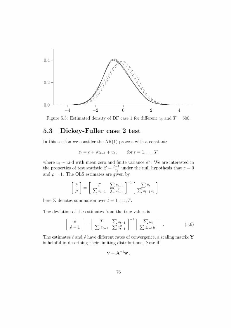
−4 −2 0 2 40.0

0.2

0.4

.................................................................................................................................................................................................

...................................................................................................................................................................................................................................................................................................................................................................................................................................................................................................................................................................................................................................................................................................................................................................................................................................................................................................................................................................................................................................................................................................................................................................................

...............................................

.............................................................................................................................................................................................................................................................................................................................................................

......................................................................................................................................................................................................................................................................................................................................................................................................................................................................................................................................................................................................................................................................................................................................................................................................................................................................

....................................

................................................................................................................................................................................................................................................................................................................................................................................................................................................................................................................................................................................................................................................................................................................................................................................................................................................................................................................................................................................................ ............. ............. ............. ............. ............. .............

.........................................................................................................................................................................

............. ..........................

..........................

..........................

..........................

..........................

..........................

............. ............. ............. ............. ............. ............. ............. ............. ............. ............. .......................... ............. ............. ............. ............. ............. ............. ............. ..........................

............................................................................................................................................................

............. ..........................

..........................

..........................

..........................

..........................

..........................

............. ............. ............. ............. ............. ............. ............. ............. ............. ............. .................... ............. ............. ............. ............. ..........................

......................................................................................................................................................................... .............

..........................

..........................

....................................................

..........................

.......................... ............. ............. ............. ............. ............. ............. ............. ...........

Figure 5.3: Estimated density of DF case 1 for different z0 and T = 500.

5.3 Dickey-Fuller case 2 test

In this section we consider the AR(1) process with a constant:

zt = c + ρzt−1 + ut , for t = 1, . . . , T,

where ut ∼ i.i.d with mean zero and finite variance σ2. We are interested inthe properties of test statistic S = ρ−1

σρunder the null hypothesis that c = 0

and ρ = 1. The OLS estimates are given by

[cρ

]=

[T

∑zt−1∑

zt−1

∑z2

t−1

]−1 [ ∑zt∑

zt−1zt

]

here Σ denotes summation over t = 1, . . . , T .

The deviation of the estimates from the true values is

[c

ρ− 1

]=

[T

∑zt−1∑

zt−1

∑z2

t−1

]−1 [ ∑ut∑

zt−1ut

]. (5.6)

The estimates c and ρ have different rates of convergence, a scaling matrix Yis helpful in describing their limiting distributions. Note if

v = A−1w ,

76

then

Yv = YA−1w

= YA−1YY−1w (5.7)

= (Y−1AY−1)−1 Y−1w.

Here we use the scaling matrix

Y =

[T 1/2 0

0 T

].

With (5.7), equation (5.6) results in

[T 1/2c

T (ρ− 1)

]=

[1 T−3/2

∑zt−1

T−3/2∑

zt−1 T−2∑

z2t−1

]−1 [T−1/2

∑ut

T−1∑

zt−1ut

](5.8)

From the proposition in paragraph 5.1 follows that the first term of the rightside of (5.8) converges to

[1 T−3/2

∑zt−1

T−3/2∑

zt−1 T−2∑

z2t−1

]D−→

[1 σ

∫W (r)dr

σ∫

W (r)dr σ2∫

W (r)2dr

]

=

[1 00 σ

] [1

∫W (r)dr∫

W (r)dr∫

W (r)2dr

] [1 00 σ

](5.9)

where the integral sign denotes integration over r from 0 to 1.

The second term of the right side of (5.8) converges to

[T−1/2

∑ut

T−1∑

zt−1ut

]D−→

[σW (1)

σ2(W (1)2 − 1)/2

]

= σ

[1 00 σ

] [W (1)

(W (1)2 − 1)/2

](5.10)

Substituting (5.9) and (5.10) into (5.8) establishes

[T 1/2c

T (ρ− 1)

]D−→

[σ 00 1

] [1

∫W (r)dr∫

W (r)dr∫

W (r)2dr

]−1 [W (1)

(W (1)2 − 1)/2

](5.11)

77

The second element in the vector in (5.11) states that

T (ρ− 1)D−→

12(W (1)2 − 1)−W (1)

∫W (r)dr∫

W (r)2dr − [∫W (r)dr

]2 . (5.12)

We like to know the properties of the t statistic S:

S =ρ− 1

σρ

,

where

σ2ρ = r2

T

[0 1

] [T

∑zt−1∑

zt−1

∑z2

t−1

]−1 [01

], (5.13)

r2T =

1

T − 2

T∑t=1

(zt − c− ρzt−1)2 .

If we multiply both sides of (5.13) by T 2, the result can be written as

T 2σ2ρ = r2

T

[0 1

]Y

[T

∑zt−1∑

zt−1

∑z2

t−1

]−1

Y

[01

]. (5.14)

From (5.8) follows

Y

[T

∑zt−1∑

zt−1

∑z2

t−1

]−1

YD−→

[1 00 σ

]−1 [1

∫W (r)dr∫

W (r)dr∫

W (r)2dr

]−1 [1 00 σ

]−1

From equation (5.14) and r2T

P→ σ2 follows

T 2σ2ρ

D−→ [0 1

] [1

∫W (r)dr∫

W (r)dr∫

W (r)2dr

]−1 [01

]

=1∫

W (r)2dr − [∫W (r)dr

]2 .

78

Finally, the asymptotic distribution of test statistic S is

S =T (ρ− 1)

[T 2σ2ρ]

1/2

D−→ (W (1)2 − 1) /2−W (1)∫

W (r)dr(∫

W (r)2dr − [∫W (r)dr

]2)1/2

. (5.15)

In conclusion, when the true model is a random walk without a constantterm (ρ = 1, c = 0) but we do estimate a constant c and of course ρ, thet test statistic S has the asymptotic distribution described by (5.15). Thistest statistic is referred to as the Dickey-Fuller case 2 test statistic.

We can find this asymptotic distribution and the corresponding critical val-ues by simulating a lot of paths W in the same way as in the precedingparagraph. The results are shown in figure 5.4 and table 5.4. Figure 5.4shows that the distribution of the DF case 2 statistic is shifted more to theleft than the DF case 1 statistic.

−6 −4 −2 0 20.0

0.2

0.4

................................................................................................................................................................................................................................

..........................................................................................................................................................................................................................................................................................................................................................................................................................................................................................................................................................................................................................................................................................................................................................................................................................................................................................................................................................................................................................................................................................................

Figure 5.4: Asymptotic density of DF case 2 test statistic.

79

Table 5.4: Critical values for DF case 1.1% 5% 10%

Hamilton -3.43 -2.86 -2.57simulation -3.43 -2.85 -2.59

These critical values belong to the asymptotic distribution (5.15), which de-scribes the distribution of the DF case 2 test statistic if the sample size Tgoes to infinity. We find the critical values for finite sample sizes T , by simu-lating paths zt as in the preceding paragraph. The only difference is the waywe calculate ρ. Again we simulate for different values of σ2. The results areshown in table 5.5, table 5.6 shows the critical values for DF case 2 accordingto Hamilton [6]. Figure 5.5 shows the estimated density of the simulated teststatistics for different values of σ2 and T = 500.

Table 5.5: Simulated critical values for DF case 2.σ2 = 1 σ2 = 5 σ2 = 10

T 1% 5% 10% 1% 5% 10% 1% 5% 10%100 -3.54 -2.85 -2.54 -3.50 -2.88 -2.56 -3.54 -2.89 -2.58250 -3.40 -2.84 -2.53 -3.46 -2.87 -2.56 -3.46 -2.86 -2.56500 -3.42 -2.86 -2.58 -3.40 -2.86 -2.55 -3.49 -2.87 -2.58

Table 5.6: Hamilton’s critical values DF case 2.T 1% 5% 10%

100 -3.51 -2.89 -2.58250 -3.46 -2.88 -2.57500 -3.44 -2.87 -2.57

80

−6 −4 −2 0 20.0

0.2

0.4

.............................................................................................................................................................................................................................

............................................................................................................................................................................................................................................................................................................................................................................................................................................................................................................................................................................................................................................................................................................................................................................................................................................................................................................................................................................................................................................................................................................

................................................

.......................................................................................................................................................................................................................................................................................................................................................................................................................................................................................................................................................................................................................................................................................................................................................................................................................................................................................................................................................................................................................................................................................................................................

...................................................

......................................................................................................................................................................................................................................................................................................................................................................................................................................................................................................................................................................................................................................................................................................................................................................................................................................................................................................................................................................................................................................................................................................................................................................................................................................

.............................................

....................................................................................................................................................................................................................................................................................................................................................................................................................................................................................................................................................................................................................................................................................................................................................................................................................................................................................................................................................................................................................................................

Figure 5.5: Estimated density of DF case 2 for different σ2 and T = 500.

Like in the preceding section, the initial term z0 does not affect the asymp-totic distribution. And fortunately, with case 2, it does not affect the dis-tribution when the sample size is finite as well. With case 2 we estimate aconstant even though it is not present in the true model, we basically fit aline which does not have to go through the origin. Then the slope of line,ρ, is not closer to one if the initial value is large, such as with case 1. Thatis why the test statistic for a large initial value is likely to be the same asthe test statistic for a small initial value. The estimated densities for initialvalues z0 = 0, 1, 10, 50, 100, 500 are shown in figure 5.6.

−6 −4 −2 0 20.0

0.2

0.4

..........................................................................................................................................

.................................................................................................................................................................................................................................................................................................................................................................................................................................................................................................................................................................................................................................................................................................................................................................................................................................................................................................................................................................................................................................................................................................................................................................................................................................................

.......................................

..................................................................................................................................................................................................................................................................................................................................................................................................................................................................................................................................................................................................................................................................................................................................................................................................................................................................................................................................................................................................................................................................................................................................................................................................

..........................................

.....................................................................................................................................................................................................................................................................................................................................................................................................................................................................................................................................................................................................................................................................................................................................................................................................................................................................................................................................................................................................................................................................................................................................................................................................................................

.........................................

.............................................................................................................................................................................................................................................................................................................................................................................................................................................................................................................................................................................................................................................................................................................................................................................................................................................................................................................................................................................................................................................................................................................................................................................

...........................................

....................................................................................................................................................................................................................................................................................................................................................................................................................................................................................................................................................................................................................................................................................................................................................................................................................................................................................................................................................................................................................................................................................................................................................................................

................................................

............................................................................................................................................................................................................................................................................................................................................................................................................................................................................................................................................................................................................................................................................................................................................................................................................................................................................................................................................................................................................................................................................

Figure 5.6: Estimated density of DF case 2 for different z0 and T = 500.

81

5.4 Dickey-Fuller case 3 test

In this section we consider again the AR(1) process with a constant

zt = c + ρzt−1 + ut , for t = 1, . . . , T, (5.16)

where ut ∼i.i.d with mean zero and finite variance σ2. We are interested inthe properties of test statistic S = ρ−1

σρunder the null hypothesis that ρ = 1

and c 6= 0.

The deviation of the estimates from the true values is

[c− cρ− 1

]=

[T

∑zt−1∑

zt−1

∑z2

t−1

]−1 [ ∑ut∑

zt−1ut

], (5.17)

here Σ denotes the summation over t = 1, . . . , T .

We examine the four different sum terms in the right side of (5.17) sepa-rately. First notice that (5.16) can be written as:

zt = z0 + c t + (u1 + u2 + . . . + ut) = z0 + c t + vt ,

wherevt = u1 + . . . + ut , for t = 1, . . . , T, with v0 = 0 .

Consider the behavior of the sum

T∑t=1

zt−1 =T∑

t=1

[z0 + c(t− 1) + vt−1] . (5.18)

The first term in (5.18) is Tz0, so divided by T is a fixed value. The secondterm is equal to

T∑t=1

c(t− 1) = (T − 1)Tc/2 .

In order to converge, this term has to be divided by T 2:

1

T 2

T∑t=1

c(t− 1) → c/2 .

82

The third term in (5.18) converges when divided by T 3/2, according to propo-sition 1 ii):

T−3/2

T∑t=1

vt−1D→ σ

∫ 1

0

W (r)dr .

The order in probability of the three terms in (5.18) is:

T∑t=1

zt−1 =T∑

t=1

z0

︸ ︷︷ ︸O(T )

+T∑

t=1

c(t− 1)

︸ ︷︷ ︸O(T 2)

+T∑

t=1

vt−1

︸ ︷︷ ︸Op(T 3/2)

.

The time trend c(t−1) asymptotically dominates the other two components:

1

T 2

T∑t=1

zt−1P→ c/2 .

In the same way, we have

T∑t=1

z2t−1 =

T∑t=1

[z0 + c(t− 1) + vt−1]2

=T∑

t=1

z20

︸ ︷︷ ︸O(T )

+T∑

t=1

c2(t− 1)2

︸ ︷︷ ︸O(T 3)

+T∑

t=1

v2t−1

︸ ︷︷ ︸Op(T 2)

+T∑

t=1

2z0c(t− 1)

︸ ︷︷ ︸O(T 2)

+T∑

t=1

2z0vt−1

︸ ︷︷ ︸Op(T 3/2)

+T∑

t=1

2c(t− 1)vt−1

︸ ︷︷ ︸Op(T 5/2)

where the order of the last term follows from

T−5/2

T∑t=1

tvt−1 = T−3/2

T∑t=1

(t/T )vt−1D→ σ

∫ 1

0

rW (r)dr .

The time trend c2(t−1)2 is the only term that does not vanish asymptoticallyif we divide by T 3:

1

T 3

T∑t=1

z2t−1

P→ c2/3

83

From the central limit theorem follows that∑T

t=1 ut is of order Op(T1/2).

And finally

T∑t=1

zt−1ut =T∑

t=1

[z0 + c(t− 1) + vt−1] ut

= z0

T∑t=1

ut

︸ ︷︷ ︸Op(T 1/2)

+T∑

t=1

c(t− 1)ut

︸ ︷︷ ︸Op(T 3/2)

+T∑

t=1

vt−1ut

︸ ︷︷ ︸Op(T )

from which

T−3/2

T∑t=1

zt−1utP→ T−3/2

T∑t=1

c(t− 1)ut .

This results in the deviation of the OLS estimates from their true valuessatisfy [

c− cρ− 1

]=

[Op(T ) Op(T

2)Op(T

2) Op(T3)

]−1 [Op(T

1/2)Op(T

3/2)

]

In this case the scaling matrix is

Y =

[T 1/2 0

0 T 3/2

]

Using (5.7) we get

[T 1/2(c− c)T 3/2(ρ− 1)

]=

[1 T−2

∑zt−1

T−2∑

zt−1 T−3∑

z2t−1

]−1 [T−1/2

∑ut

T−3/2∑

zt−1ut

](5.19)

where the first term of the righthand side converges to

[1 T−2

∑zt−1

T−2∑

zt−1 T−3∑

z2t−1

]P−→

[1 c/2

c/2 c2/3

]= A . (5.20)

The second term of (5.19) satisfies

[T−1/2

∑ut

T−3/2∑

zt−1ut

]=

[T−1/2

∑ut

T−3/2∑

c(t− 1)ut

]+ op(1)

84

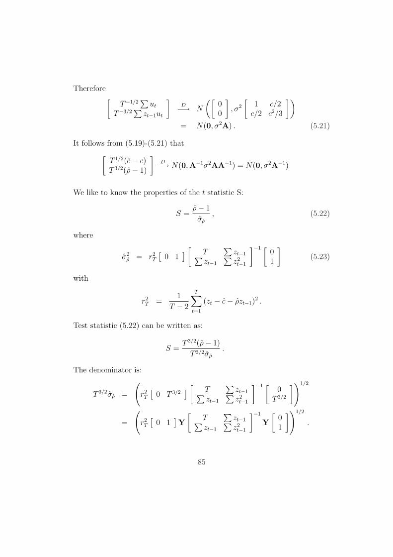
Therefore[

T−1/2∑

ut

T−3/2∑

zt−1ut

]D−→ N

([00

], σ2

[1 c/2

c/2 c2/3

])

= N(0, σ2A) . (5.21)

It follows from (5.19)-(5.21) that

[T 1/2(c− c)T 3/2(ρ− 1)

]D−→ N(0,A−1σ2AA−1) = N(0, σ2A−1)

We like to know the properties of the t statistic S:

S =ρ− 1

σρ

, (5.22)

where

σ2ρ = r2

T

[0 1

] [T

∑zt−1∑

zt−1

∑z2

t−1

]−1 [01

](5.23)

with

r2T =

1

T − 2

T∑t=1

(zt − c− ρzt−1)2 .

Test statistic (5.22) can be written as:

S =T 3/2(ρ− 1)

T 3/2σρ

.

The denominator is:

T 3/2σρ =

(r2T

[0 T 3/2

] [T

∑zt−1∑

zt−1

∑z2

t−1

]−1 [0

T 3/2

])1/2

=

(r2T

[0 1

]Y

[T

∑zt−1∑

zt−1

∑z2

t−1

]−1

Y

[01

])1/2

.

85

We have already shown that

Y

[T

∑zt−1∑

zt−1

∑z2

t−1

]−1

Y =

(Y−1

[T

∑zt−1∑

zt−1

∑z2

t−1

]Y−1

)−1

=

[1 T−2

∑zt−1

T−2∑

zt−1 T−3∑

z2t−1

]

converges in probability towards A.

Because r2T

P→ σ2, the denominator converges towards

T 3/2σρP−→ σc/

√3 .

Thus, the test statistic S is asymptotically Gaussian. The regressor yt−1 isasymptotically dominated by the time trend c(t− 1). In large samples, it isas if the explanatory variable yt−1 were replaced by the time trend c(t− 1).That is why the asymptotic properties of c and ρ are the same as those forthe deterministic time trend regression. Therefore, for finite T test statisticS has a t distribution.

In conclusion, when the true model is a random walk with a constant term(ρ = 1, c 6= 0) and we estimate both ρ and c then the t test statistic S hasan asymptotic distribution equal to the standard Gaussian distribution:

SD−→ N(0, 1)

This test statistic is referred to as the Dickey-Fuller case 3 test statistic. Thecritical values for T →∞ are given in table 5.7.

Table 5.7: Critical values for DF case 3.1% 5% 10%

N(0, 1) -2.33 -1.64 -1.28

For finite T the Dickey-Fuller case 3 test statistic is t distributed, but thedegrees of freedom are large so it is almost standard normal. We can alsofind the critical values for finite T , by simulating paths zt as in the precedingparagraphs. Again we simulate for different values of σ2. The results areshown in table 5.8. Figure 5.7 shows the estimated density of the simulatedtest statistics for different values of σ2 while T = 500 and c = 2.5, the stan-dard normal density is also displayed.

86

Table 5.8: Simulated critical values for DF case 3.σ2 = 1 σ2 = 5 σ2 = 10

T 1% 5% 10% 1% 5% 10% 1% 5% 10%100 -2.36 -1.76 -1.37 -2.51 -1.82 -1.46 -2.48 -1.84 -1.49250 -2.37 -1.68 -1.33 -2.41 -1.74 -1.35 -2.40 -1.79 -1.40500 -2.38 -1.75 -1.33 -2.41 -1.69 -1.35 -2.45 -1.76 -1.38

−4 −2 0 2 40.0

0.2

0.4

...........................................................................................................................................................................................

...................................

......................................................................................................................................................................................................................................................................................................................

.......................................................................................................................................................................................................................................................................................................................................................................................................................................................................................................................................................................................................................................................................................................................................................................................................................

....................................

..........................................................................................................................................................................................................................................................................................................................................................................................................................................................................................................................................................................................................................................................................................................................................................................................................................................................................................................................................................................................................................................................................................

........................................................

..................................................................................................................................................................................................................................................................................................................................................................................................................................................................................................................................................................................................................................................................................................................................................................................................................................................................................................................................................................................................................................................................................................................................................

..............................................

.........................................................................................................................................................................................................................................................................................................................................................................................................................................................................................................................................................................................................................................................................................................................................................................................................................................................................................................................................

Figure 5.7: Estimated density of DF case 3 for different σ2 and T = 500.

To see if the value of the constant c has an impact on finite sample distri-bution of the Dickey-Fuller case 3 statistic, we simulate paths zt for c =0.1, 0.5, 1, 2.5, 10. The results are shown in figure 5.8, the standard normaldensity is also displayed. The graph most left corresponds with c = 0.1.

87

−4 −2 0 2 40.0

0.2

0.4

..................................................................................................................................................................................

....................................

............................................................................................................................................................................................................................................................................................................................

....................................................................................................................................................................................................................................................................................................................................................................................................................................................................................................................................................................................................................................................................................................................................................................................................

.................................

..............................................................................................................................................................................................................................................................................................................................................................................................................................................................................................................................................................................................................................................................................................................................................................................................................................................................................................................................................................................................................................................................................................................................................

....................................................

.............................................................................................................................................................................................................................................................................................................................................

..................................................................................................................................................................................................................................................................................................................................................................................................................................................................................................................................................................................................................................................................................................................................................................................................................................

.......................................

...................................................................................................................................................................................................................................................................................................................

..........................................................................................................................................................................................................................................................................................................................................................................................................................................................................................................................................................................................................................................................................................................................................................

.................................

.............................................................................................................................................................................................................................................................................................................................

...........................................................................................................................................................................................................................................................................................................................................................................................................................................................................................................................................................................................................................................................................................................................................................................................................................................................................................................................................................................................

...............................................................................................................................................................................................................................................................................................................................................................................................................................................................................................................................................................................................................................................................................................................................................................................................................................................................................................................................................................................................................................................................................................................................................................................................................................................................................................................................................................................................................................................................................

Figure 5.8: Estimated density of DF case 3 for different c and T = 500.

It looks like a small value of c causes a shift to the left. In figure 5.9 theestimated distribution for c = 0.01, 0.05, 0.1 is plotted with solid lines. Thedashed line is the distribution of case 1 and the dotted line is the distribu-tion of case 2. For c = 0.01 the estimated density is almost the same as thedensity found for case 2. This makes sense because the steps taken in thecase 2 en case 3 tests are exactly the same, the only difference is the truemodel for case 2 has no constant and for case 3 it has. So for a decreasingconstant the case 3 test statistic converges to the case 2 statistic. The otherway around is also valid: for an increasing constant, in absolute value, thecase 2 test statistic converges to the case 3 statistic because the tests are thesame but now there is a constant in the true model.

−4 −2 0 2 40.0

0.2

0.4

.............................................................................................

.......................................................................................................................................................................................................................................................................................................................................................................................................................................................................................................................................................................................................................................................................................................................................................................................................................................................................................................................................................................................................................................................

..............................................

.................................................................................................................................................................................................................................................................................................................................................

.....................................................................................................................................................................................................................................................................................................................................................................................................................................................................................................................................................................................................................................................................................................................................

..........................................................................................................................................................................................................................................................................................................................................................

.......................................................................................................................................................................................................................................................................................................................................................................................................................................................................................................................................................................................... ............. ............. ............. ............. ............. ..........................

............................................................................................................................................................ .............

..........................

..........................

..........................

..........................

..........................

..........................

............. ............. ............. ............. ............. ............. ............. ............. ............. .....................................................

.........................................................................................................................................................................................................................................................................................................................................................................................................................................................................................................................................................

Figure 5.9: Estimated density of DF case 3 for small c and T = 500.

88

To be consistent, we also simulate for several different initial values z0. Fig-ure 5.10 shows the results for z0 = 0, 1, 10, 50, 100, 500 while T = 500 andc = 2.5. The figure suggests that the initial value z0 does not affect thedensity of the test statistic for finite sample sizes.

−4 −2 0 2 40.0

0.2

0.4

............................................................................................................................................................................................

...................................

..................................................................................................................................................................................................................................................................................................................

.............................................................................................................................................................................................................................................................................................................................................................................................................................................................................................................................................................................................................................................................................................................................................................................................................................

..................................

.................................................................................................................................................................................................................................................................................................................

...................................................................................................................................................................................................................................................................................................................................................................................................................................................................................................................................................................................................................................................................................................................................................................................................................................................

....................................

........................................................................................................................................................................................................................................................................................................................................................................................................................................................................................................................................................................................................................................................................................................................................................................................................................................................................................................................................................................................................................................................................

.................................................

...............................................................................................................................................................................................................................................................................................................................................................................................................................................................................................................................................................................................................................................................................................................................................................................................................................................................................................................................................................................................................................................

....................................................

......................................................................................................................................................................................................................................................................................................................................

..........................................................................................................................................................................................................................................................................................................................................................................................................................................................................................................................................................................................................................

Figure 5.10: Estimated density of DF case 3 for different z0

There also exist a case 4 for the Dickey-Fuller test, this includes a determin-istic time trend in the true model. We are not interested in spread processeswith deterministic trends so we do not discuss this case.

5.5 Power of the Dickey-Fuller tests

In this section we investigate how ’powerful’ the different cases of the Dickey-Fuller test are. We generate paths zt which do not have a unit root, ρ < 1in

zt = c + ρzt−1 + ut

and see if the different tests see it as stationary. In other words whetherthe outcome of the test is to reject the null hypothesis that there is a unitroot, ρ = 1. For different values of c and z0 we generate 1,000 paths zt,t = 0, . . . , T where T = 500 and count the number of rejections. The resultsare presented in tables.

89

First we summarize the previous sections.

Case 1: The true model of case 1 is zt = zt−1 + ut where ut ∼ i.i.d withmean zero and finite variance σ2. We estimate the model zt = ρzt−1 + ut.The critical values for test statistic S = ρ−1

σρwhen T = 500 are

1% 5% 10%-2.58 -1.95 -1.62

Case 2: The true model of case 2 is zt = zt−1 +ut where ut ∼ i.i.d with meanzero and finite variance σ2. We estimate the model zt = c + ρzt−1 + ut. Thecritical values for test statistic S = ρ−1

σρwhen T = 500 are

1% 5% 10%-3.44 -2.87 -2.57

Case 3: The true model of case 3 is zt = c + zt−1 + ut where ut ∼ i.i.dwith mean zero and finite variance σ2 and c 6= 0. We estimate the modelzt = c+ρzt−1+ut. The critical values for test statistic S = ρ−1

σρwhen T = 500

are

1% 5% 10%-2.33 -1.64 -1.28

We have seen that the initial value z0 does affect the finite sample distribu-tion of Dickey-Fuller case 1 but does not affect case 2 and case 3. The valueof c does affect the distribution of case 3: as c becomes smaller the distribu-tion converges to the distribution of case 2. IMC has provided 10 pairs, therange of c of these 10 pairs is (−0.01, 0.1). The absolute initial value z0 ofthe 10 pairs is less than 1.5 for 9 of the 10 pairs. With one pair z0 is 106. Sowe are interested in the power of the three tests for small values of c and z0,but we will also look at large values of z0.

90

We start with generating paths with c = 0 and z0 = 0. In all followingtables T = 500, σ = 1 and the number of generated paths is 1,000. Table5.9 shows the number of rejections for the different tests and different valuesof ρ. For ρ = 1 we have simulated paths under the null hypothesis of case1 and case 2, the number of rejections are in line with what we expected.The case 3 test does not perform very well, with ρ = 1 it rejects the nullhypothesis that ρ = 1 632 out of 1,000 times on the 10% level. For ρ justunder 1, the case 1 test performs better than the case 2 test.

Table 5.9: Number of rejections, c = 0, z0 = 0.Case 1 Case 2 Case 3

ρ 1% 5% 10% 1% 5% 10% 1% 5% 10%0.9 1000 1000 1000 1000 1000 1000 1000 1000 10000.95 986 1000 1000 746 966 997 1000 1000 10000.975 479 910 982 135 427 663 835 991 10000.99 73 310 528 22 116 205 338 771 9180.995 41 144 274 21 77 148 231 617 783

1 10 48 96 12 54 105 171 456 6321.01 0 0 0 0 0 0 1 4 12

Table 5.10 shows the number of rejections for generated paths with c = 0 andz0 = 100. For ρ = 1 we simulated under the null hypothesis of case 1 and2, the number of rejections for case 1 is small. This was expected becauseof figure 5.3. Again, the case 3 test does not perform very well when ρ = 1.The case 1 and 2 tests do perform well, with ρ slightly less than 1 they rejectthe null of an unit root.

91

Table 5.10: Number of rejections, c = 0, z0 = 100.Case 1 Case 2 Case 3

ρ 1% 5% 10% 1% 5% 10% 1% 5% 10%0.99 1000 1000 1000 1000 1000 1000 1000 1000 10000.995 1000 1000 1000 406 683 805 874 974 995

1 8 26 47 10 52 106 157 461 6311.01 0 0 0 0 0 0 0 0 0

Table 5.11 shows the number of rejections for c = 0.1 and z0 = 0. For ρ = 1we have simulated under the null hypothesis of case 3 but the case 3 test stillrejects to many times. Because the null is fulfilled we expect the numberof rejections to be around 10, 50 and 100 for the 1%, 5% and 10% levelsrespectively. In figure 5.8 we already saw that the case 3 test is dependentof the value of c, when c = 0.1 the distribution of the case 3 test statisticis shifted to the left compared to its asymptotic distribution. We see thatwith this setting the case 2 test performs more or less the same as with c = 0and z0 = 0 except when ρ = 1, in which case it rejects less. The null is notsatisfied for the case 2 test, so this is not a bad outcome. The less rejectionsfor ρ = 1 the better. The case 1 test performs less compared to case 2 testas well as the setting c = 0 and z0 = 0.

Table 5.11: Number of rejections, c = 0.1, z0 = 0.Case 1 Case 2 Case 3

ρ 1% 5% 10% 1% 5% 10% 1% 5% 10%0.9 1000 1000 1000 1000 1000 1000 1000 1000 10000.95 758 968 997 848 995 1000 999 1000 10000.975 111 434 675 157 476 729 831 996 10000.99 6 37 87 39 142 262 376 765 9170.995 0 7 20 18 90 158 257 599 768

1 0 2 3 5 18 37 73 217 3291.01 0 0 1 0 0 0 2 8 9

92

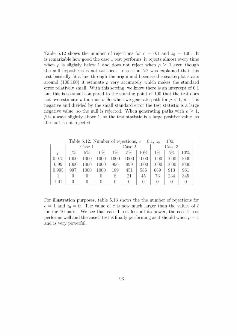
Table 5.12 shows the number of rejections for c = 0.1 and z0 = 100. Itis remarkable how good the case 1 test performs, it rejects almost every timewhen ρ is slightly below 1 and does not reject when ρ ≥ 1 even thoughthe null hypothesis is not satisfied. In section 5.2 was explained that thistest basically fit a line through the origin and because the scatterplot startsaround (100,100) it estimate ρ very accurately which makes the standarderror relatively small. With this setting, we know there is an intercept of 0.1but this is so small compared to the starting point of 100 that the test doesnot overestimate ρ too much. So when we generate path for ρ < 1, ρ − 1 isnegative and divided by the small standard error the test statistic is a largenegative value, so the null is rejected. When generating paths with ρ ≥ 1,ρ is always slightly above 1, so the test statistic is a large positive value, sothe null is not rejected.

Table 5.12: Number of rejections, c = 0.1, z0 = 100.Case 1 Case 2 Case 3

ρ 1% 5% 10% 1% 5% 10% 1% 5% 10%0.975 1000 1000 1000 1000 1000 1000 1000 1000 10000.99 1000 1000 1000 996 999 1000 1000 1000 10000.995 997 1000 1000 189 451 586 689 913 961

1 0 0 0 8 21 45 73 234 3451.01 0 0 0 0 0 0 0 0 0

For illustration purposes, table 5.13 shows the the number of rejections forc = 1 and z0 = 0. The value of c is now much larger than the values of cfor the 10 pairs. We see that case 1 test lost all its power, the case 2 testperforms well and the case 3 test is finally performing as it should when ρ = 1and is very powerful.

93

Table 5.13: Number of rejections, c = 1, z0 = 0.Case 1 Case 2 Case 3

ρ 1% 5% 10% 1% 5% 10% 1% 5% 10%0.9 0 0 0 1000 1000 1000 1000 1000 10000.95 0 0 0 1000 1000 1000 1000 1000 10000.975 0 0 0 998 1000 1000 1000 1000 10000.99 0 0 0 1000 1000 1000 1000 1000 10000.995 0 0 0 997 1000 1000 1000 1000 1000

1 0 0 0 1 7 12 13 59 1191.01 0 0 0 0 0 0 0 0 0

This section clearly indicates that the Dickey-Fuller case 3 test is not the onewe should use when testing pairs for cointegration. Unfortunately it does notclearly distinguish case 1 and case 2. Case 1 performs better for c = 0, z0 = 0and c = 0, z0 = 100 and c = 0.1, z0 = 100, but case 2 performs better forc = 0.1, z0 = 0 which is most seen in the 10 pairs. In the remainder of thisreport we will focus on the case 2 test because of Hamilton’s view given insection 4.3 and because this section does not clearly indicate to do otherwise.Another possible reason to use case 2 instead of case 1 could be that thatthe first step of the Engle-Granger method, which is a linear regression toestimate α, influences the power of the two tests. This will be considered inchapter 6.

5.6 Augmented Dickey-Fuller test

So far we discussed the properties of the estimated coefficients for a first-order autoregression when there is a unit root. In this section we discuss thedistribution of the estimated coefficients for a p-th order autoregression.Recall that the Augmented Dickey-Fuller test tests

H0 : zt ∼ I(1) against H1 : zt ∼ I(0) , (5.24)

when zt is assumed to follow an AR(p) model

zt = c + φ1zt−1 + · · ·+ φpzt−p + ut , (5.25)

94

where ut ∼ i.i.d(0, σ2).

This model can be written as

zt = c + ρzt−1 + β1∆zt−1 + · · ·+ βp−1∆zt−p+1 + ut , (5.26)

with

ρ = φ1 + φ2 + · · ·+ φp ,

βi = −(φi+1 + · · ·+ φp) , for i = 1, . . . , p− 1 .

The null hypothesis is that the autoregressive polynomial

1− φ1x− φ2x2 − · · · − φpx

p = 0 ,

has exactly one unit root and all other roots lie outside the unit circle. Thesingle unit root gives us:

1− φ1 − φ2 − · · · − φp = 0

i.e., ρ = 1. This implies

1− φ1x− · · · − φpxp = (1− β1x− · · · − βp−1x

p−1)(1− x) . (5.27)

Of the p values of x that make the left side of (5.27) zero, one is x = 1 andall other roots are assumed to be outside the unit circle. The same must betrue for the right side as well, meaning all roots of

1− β1x− · · · − βp−1xp−1 = 0 .

lie outside the unit circle. So, (5.24) is equivalent to

H0 : ρ = 1 against H1 : ρ < 1 .

We are interested in the properties of test statistic S = ρ−1σρ

in the three cases:

Case 1: The true process of zt is (5.26) with c = 0 and ρ = 1,the model estimated is (5.26) except for c.

Case 2: The true process of zt is (5.26) with c = 0 and ρ = 1,the model estimated is (5.26).

Case 3: The true process of zt is (5.26) with c 6= 0 and ρ = 1,the model estimated is (5.26).

95

We can derive the asymptotic properties in a similar manner as in the pre-ceding sections. To keep this section from being to tedious, we only derivethe properties for case 2. We state the outcomes for case 1 and case 3 at theend of this section, the derivations can be found in Hamilton [6].

Before deriving the properties for Augmented Dickey-Fuller case 2, we firststate a proposition.

Proposition 2:Let vt =

∑∞j=0 θjut−j, where

∑∞j=0 j · | θj| < ∞ and ut is an i.i.d sequence

with mean zero, variance σ2, and finite fourth moment. Define

γj = E(vtvt−j) = σ2

∞∑s=0

θsθs+j , for j = 0, 1, . . . , (5.28)

λ = σ

∞∑j=0

θj , (5.29)

zt = v1 + v2 + · · ·+ vt , for t = 1, 2, . . . , T , (5.30)

with z0 = 0. Then

(i) T−1∑T

t=1 vtvt−jP→ γj for j = 0, 1, . . .

(ii) T−1∑T

t=1 zt−1vt−jD→

12(λ2W (1)2 − γ0)

12(λ2W (1)2 − γ0)

+γ0 + · · ·+ γj−1

for j = 0

for j = 1, 2, . . .

(iii) T−3/2∑T

t=1 zt−1D→ λ

∫ 1

0W (r) dr .

(iv) T−2∑T

t=1 z2t−1

D→ λ2∫ 1

0W (r)2 dr .

(v) T−1/2∑T

t=1 vtD→ λW (1) .

(vi) T−1∑T

t=1 zt−1utD→ 1

2σλ(W (1)2 − 1) .

The proof of this proposition can also found in [6].

96

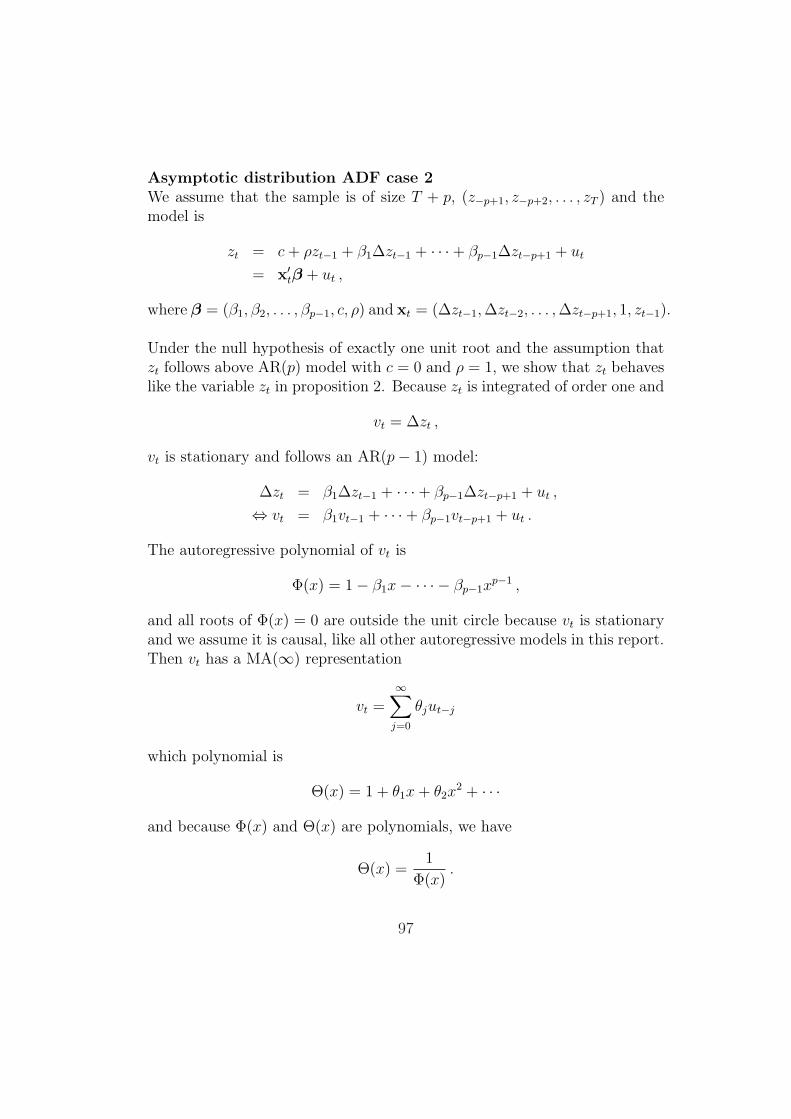
Asymptotic distribution ADF case 2We assume that the sample is of size T + p, (z−p+1, z−p+2, . . . , zT ) and themodel is

zt = c + ρzt−1 + β1∆zt−1 + · · ·+ βp−1∆zt−p+1 + ut

= x′tβ + ut ,

where β = (β1, β2, . . . , βp−1, c, ρ) and xt = (∆zt−1, ∆zt−2, . . . , ∆zt−p+1, 1, zt−1).

Under the null hypothesis of exactly one unit root and the assumption thatzt follows above AR(p) model with c = 0 and ρ = 1, we show that zt behaveslike the variable zt in proposition 2. Because zt is integrated of order one and

vt = ∆zt ,

vt is stationary and follows an AR(p− 1) model:

∆zt = β1∆zt−1 + · · ·+ βp−1∆zt−p+1 + ut ,

⇔ vt = β1vt−1 + · · ·+ βp−1vt−p+1 + ut .

The autoregressive polynomial of vt is

Φ(x) = 1− β1x− · · · − βp−1xp−1 ,

and all roots of Φ(x) = 0 are outside the unit circle because vt is stationaryand we assume it is causal, like all other autoregressive models in this report.Then vt has a MA(∞) representation

vt =∞∑

j=0

θjut−j

which polynomial is

Θ(x) = 1 + θ1x + θ2x2 + · · ·

and because Φ(x) and Θ(x) are polynomials, we have

Θ(x) =1

Φ(x).

97

All p−1 roots, which is a finite number of roots, of Φ(x) are outside the unitcircle, so there exists an ε > 0 such that the modus of all roots are largerthan 1 + ε, so Φ(x) 6= 0 for |x| < 1 + ε. Within the radius of convergence1 + ε, the analytic function Θ(x) is differentiable:

Θ′(x) =∞∑

j=1

jθjxj−1 .

And because it is absolutely convergent within its radius of convergence,particularly in point 1, we have

∞∑j=1

j · |θj| < ∞ .

This shows we can use proposition 2 without making any further assumptions.

The deviation of the OLS estimate β from the true value β is given by

β − β =

[T∑

t=1

xtx′t

]−1 [T∑

t=1

xtut

]. (5.31)

With vt = zt − zt−1, the terms in (5.31) are

T∑t=1

xtx′t =

∑v2

t−1 · · · ∑vt−1vt−p+1

∑vt−1

∑vt−1zt−1∑

vt−2vt−1 · · · ∑vt−2vt−p+1

∑vt−2

∑vt−2zt−1

... · · · ......

...∑vt−p+1vt−1 · · · ∑

v2t−p+1

∑vt−p+1

∑vt−p+1zt−1∑

vt−1 · · · ∑vt−p+1 T

∑zt−1∑

zt−1vt−1 · · · ∑zt−1vt−p+1

∑zt−1

∑z2

t−1

,

T∑t=1

xtut =

∑vt−1ut...∑

vt−p+1ut∑ut∑

zt−1ut

.

98

Like in the derivation of DF case 2 we need a scaling matrix, in this sectionwe use the following (p + 1)× (p + 1) scaling matrix:

Y =

√T 0 · · · 0 0

0√

T · · · 0 0...

... · · · √T 0

0 0 · · · 0 T

With multiplying (5.31) by the scaling matrix Y and using (5.7) we get

Y(β − β) =

Y−1

[T∑

t=1

xtx′t

]Y−1

−1 Y−1

[T∑

t=1

xtut

](5.32)

Consider the matrix Y−1∑

xtx′tY

−1. Elements in the upper left (p × p)block of

∑xtx

′t are divided by T , the first p elements of the (p + 1)th row

or (p + 1)th column are divided by T 3/2 and the element at the lower rightcorner is divided by T 2. Moreover,

T−1∑

vt−ivi−jP→ γ|i−j| from proposition 2(i) ,

T−1∑

vt−jP→ E(vt−j) = 0 from the law of large numbers ,

T−3/2∑

zt−1vt−jP→ 0 from proposition 2(ii) ,

T−3/2∑

zt−1D→ λ

∫W (r) dr from proposition 2(iii) ,

T−2∑

z2t−1

D→ λ2∫

W (r)2 dr from proposition 2(iv) ,

where

γj = E(∆zt ∆zt−j) ,

λ = σ/(1− β1 − · · · − βp−1) ,

σ2 = E(u2t ) ,

and the integral sign denotes integration over r from 0 to 1. Thus,

Y−1

[T∑

t=1

xtx′t

]Y−1 D−→

γ0 · · · γp−2 0 0... · · · ...

......

γp−2 · · · γ0 0 00 · · · 0 1 λ

∫W (r) dr

0 · · · 0 λ∫

W (r) dr λ2∫

W (r)2 dr

=

[V 00 Q

],

99

with

V =

γ0 γ1 · · · γp−2

γ1 γ0 · · · γp−3...

... · · · ...γp−2 γp−3 · · · γ0

,

Q =

[1 λ

∫W (r) dr

λ∫

W (r) dr λ2∫

W (r)2 dr

]. (5.33)

Next, consider the second term in the right side of(5.32)

Y−1

[T∑

t=1

xtut

]=

T−1/2∑

vt−1ut...

T−1/2∑

vt−p+1ut

T−1/2∑

ut

T−1∑

zt−1ut

. (5.34)

The first p− 1 elements of this vector satisfy the central limit theorem. Thisis because these elements are

√T times the sample mean of a martingale

difference sequence whose covariance matrix is σ2V, but this is not discussedfurther. The result is

T−1/2∑

vt−1ut...

T−1/2∑

vt−p+1ut

D→ h1 ∼ N(0, σ2V) .

The distribution of the last two elements in (5.34) can be obtained fromstatements (v) en (vi) of proposition 2:

[T−1/2

∑ut

T−1∑

zt−1ut

]D→ h2 ∼

[σW (1)

12σλ(W (1)2 − 1)

]. (5.35)

This gives that the deviation of the OLS estimate from its true value is

Y(β − β)D→

[V 00 Q

]−1 [h1

h2

]=

[V−1h1

Q−1h2

]. (5.36)

100

The last two elements of β are c and ρ, which are the constant term andthe coefficient on the I(1) regressor, zt−1. From (5.33),(5.35) and (5.36),their limiting distribution is given by

[T 1/2 0

0 T

] [c

ρ− 1

]D→

[σ 00 σ/λ

] [1

∫W (r) dr∫

W (r) dr∫

W (r)2 dr

]−1 [W (1)

12(W (1)2 − 1)

](5.37)

The t test statistic S of the null hypothesis that ρ = 1 is

S =ρ− 1

σρ

=ρ− 1

r2Te(

∑xtx′t)−1e1/2

,

where e denotes a p + 1 vector with unity in the last postition and zeroselsewhere. Multiplying the numerator and the denominator by T results in

S =T (ρ− 1)

r2TeY(

∑xtx′t)−1Ye1/2

.

But

eY(∑

xtx′t

)−1

Ye = eY

(∑xtx

′t

)Y

−1

e

D→ e′[

V−1 00 Q−1

]e (5.38)

=1

λ2∫

W (r)2 dr − (∫W (r) dr

)2 .

By (5.37) we have

T (ρ− 1)D→ (σ/λ)

12(W (1)2 − 1)−W (1)

∫W (r) dr∫

W (r)2 dr − (∫W (r) dr

)2 . (5.39)

Using (5.38) and (5.39) together with r2T

P→ σ2, we finally get

SD→

12(W (1)2 − 1)−W (1)

∫W (r) dr

(∫W (r)2 dr − [∫

W (r) dr]2

)1/2, (5.40)

101

which is exactly the same as the asymptotic distribution of the Dickey-Fullercase 2 test statistic. So the critical values are the same as in table 5.4 insection 5.3 without making any corrections for the fact that lagged valuesof ∆zt are included in the regression. This is also true for the other cases,Augmented Dickey-Fuller case 1 test statistic has the same asymptotic dis-tribution as Dickey-Fuller case 1 and ADF case 3 the same as DF case 3.

Like in the preceding sections we can simulate the density of the test statisticfor finite sample sizes, we show the results for the case 2 test when p = 2.We simulate for different values of σ when T = 500 and β1 = −0.1, andnaturally ρ = 1, c = 0. We took this value for β1 because this value is seena few times in the 10 pairs IMC provided. The estimated densities of 5,000simulated test statistics for σ2 = 1, 5, 10 are shown in figure 5.11. Also theasymptotic density we found for the case 2 test, figure 5.4, is plotted witha dashed line. The different graphs coincide nicely. With this setting, the’original’ AR model with lagged terms instead of differenced terms is:

zt = 0.9zt−1 + 0.1zt−2 + ut .

The autoregressive polynomial

1− 0.9x− 0.1x2 = 0 ,

has roots 1 and −10, so the assumption of exactly one unit root is fulfilled.

−6 −4 −2 0 20.0

0.2

0.4

.........................................................................................................................................................................

......................................................................................................................................................................................................................................................................................................................................................................................................................................................................................................................................................................................................................................................................................................................................................................................................................................................................................................................................................................................................................................................................................

......................................

..........................................................................................................................................................................................................................................................................................................................................................................................................................................................................................................................................................................................................................................................................................................................................................................................................................................................................................................................................................................................................................................................................................

.................................................................................................................................................................................................................................................................................................................................................................................................................................................................................................................................................................................................................................................................................................................................................................................................................................................................................................................................................................................................................. .......... .......... .......... .......... .......... .......... .......... .......... ..........

....................

..........................................................................................................................................................................

.............................................................................................................................................................................................. .......... .......... .......... .......... .......... .......... .......... .......... .......... .......... ..........

Figure 5.11: Estimated density of ADF case 2 for different σ2, T = 500 andβ1 = −0.1.

102

To see what influence β1 has we also vary its value while keeping σ2 fixed at1. The results for β1 = −0.9,−0.5, 0, 0.5, 0.9, 1 are shown in figure 5.12. Theawkward graph corresponds with β1 = 1, the ’original’ AR model is:

zt = 2zt−1 − zt−2 + ut

The autoregressive polynomial

1− 2x + x2 = 0

has twice root 1, so there are two unit roots. That is probably why the graphfor β1 = 1 does not look like the other ones. For the other values of β1 the as-sumption of exactly one unit root is fulfilled. The values of β1 for the 10 pairswhen an AR(2) model is fit on the spread process are in a range of (-0.25,0.1).

−6 −4 −2 0 2 40.0

0.2

0.4

......................................................................................................................

............................................................................................................................................................................................................................................................................................................................................................................................................................................................................................................................................................................................................................................................................................................................................................................................................................................................................................................................................................................................................................................................

...............................................................................................................................................................................................................................................................................................................................................................................................................................................................................................................................................................................................................................................................................................................................................................................................................................................................................................................................................................................................

...............................................................................................................................................................................................................................................................................................................................................................................................................................................................................................................................................................................................................................................................................................................................................................................................................................................................................................................................................................................................................................................................................................

........................................

.............................................................................................................................................................................................................................................................................................................................................................................................................................................................................................................................................................................................................................................................................................................................................................................................................................................................................................................................................................................................................................................................................................

...........................................................................................................................................................................................................................................................................................................................................................................................................................................................................................................................................................................................................................................................................................................................................................................................................................................................................................................................................................................................................................................................................................................

.........................................

.....................................................................................................................................................................

........................................................................................................................................................

........................................................................................................................................................................................................................................................................................................................................................................................................................................

Figure 5.12: Estimated density of ADF case 2 for different β1, T = 500 andσ2 = 1.

103

We also show the results for two higher order models. First p = 3, fig-ure 5.13 shows the estimated densities for three different settings of β1 andβ2. We take β2 equal to -0.1 and β1 is -0.2, -0.1 and 0.1 successively, theseare also values seen with the 10 pairs. For these values the autoregressivepolynomial has exactly one unit root and the other roots are outside theunit circle, so the null hypothesis is satisfied. Also the graph of figure 5.4 isdisplayed, again they coincide nicely.

−6 −4 −2 0 20.0

0.2

0.4

...........................................................................................................................................

...............................................................................................................................................................................................................................................................................................................................................................................................................................................................................................................................................................................................................................................................................................................................................................................................................................................................................................................................................................................................................................................................................................................................................

...............................................

......................................................................................................................................................................................................................................................................................................................................................................................................................................................................................................................................................................................................................................................................................................................................................................................................................................................................................................................................................................................................................................................................................................

.............................................

................................................................................................................................................................................................................................................................................................................................................................................................................................................................................................................................................................................................................................................................................................................................................................................................................................................................................................................................ ............. ............. ............. ............. ............. ............. ............. .............

......................................................................................................................................................................... .............

..............................................................................

..........................

..........................

.......................... ............. ............. ............. ............. ............. ............. ............. ............. .............

Figure 5.13: Estimated density of ADF case 2 for different β1 and β2, T = 500and σ2 = 1.

Lastly, we consider p = 5. Figure 5.14 shows the estimated densities forthree parameter settings:

Setting 1 : β1 = −0.3 β2 = −0.2 β3 = −0.1 β4 = −0.05Setting 2 : β1 = −0.1 β2 = −0.1 β3 = −0.1 β4 = −0.1Setting 3 : β1 = 0.1 β2 = −0.1 β3 = 0.1 β4 = 0.05

These three settings also represents most of the 10 pairs and that the nullhypothesis is satisfied was checked with Maple. We see that the densitiesshow more dispersion and do not coincide with the asymptotic density asnicely as for the lower order models above.

104

−6 −4 −2 0 20.0

0.2

0.4

...............................................................................................................

...................................................................................................................................................................................................................................................................................................................................................................................................................................................................................................................................................................................................................................................................................................................................................................................................................................................................................................................................................................................................................................................................................................................................................................................

..........................................

...........................................................................................................................................................................................................................................................................................................................................

.................................................................................................................................................................................................................................................................................................................................................................................................................................................................................................................................................................................................................................................................................................................................

......................................

.................................................................................................................................................................................................................................................................................................................................................................................................................................................................................................................................................................................................................................................................................................................................................................................................................................................................................................................. ............. ............. ............. ............. ............. ............. ............. .............

......................................................................................................................................................................... .............

..............................................................................

..........................

..........................

.......................... ............. ............. ............. ............. ............. ............. ............. ............. .............

Figure 5.14: Estimated density of ADF case 2 for different β1, T = 500 andσ2 = 1.

In the next section we look again at all these models to see if the power ofthe Augmented Dickey-Fuller case 2 test is influenced by the value of p.

5.7 Power of the Augmented Dickey-Fuller

case 2 test

In this section we briefly look at how much influence the value of p, the orderof the autoregressive model, has on the power of the Augmented Dickey-Fuller case 2 test. As in section 5.5 we generate 1,000 paths for differentvalues of ρ and see how many times the test rejects the null hypothesis of aunit root.

We start with p = 2, so the paths are generated according to the model

zt = ρzt−1 + β1∆zt−1 + ut ,

for we take ut i.i.d standard Gaussian random variables, sample size T = 500and z0 = 0. Table 5.14 shows the number of rejections for several values ofρ and β1. We use values of β1 which are seen with the 10 pairs IMC pro-vided. When ρ = 1 the null hypothesis is satisfied, the other roots of theautoregressive polynomial lie outside the unit circle, they are -4, -10 and 10respectively for β1 = −0.25,−0.1, 0.1. We see that under the null hypothesisthe test behaves as expected. The power is quite similar to the Dickey-Fullercase 2 test in table 5.9. The power is better for the positive value of β1.

105

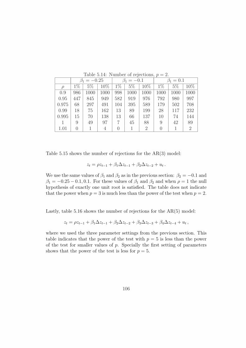
Table 5.14: Number of rejections, p = 2.β1 = −0.25 β1 = −0.1 β1 = 0.1

ρ 1% 5% 10% 1% 5% 10% 1% 5% 10%0.9 986 1000 1000 998 1000 1000 1000 1000 10000.95 447 845 949 582 919 976 792 980 9970.975 68 297 491 104 395 589 179 502 7080.99 18 75 162 13 89 199 28 117 2320.995 15 70 138 13 66 137 10 74 144

1 9 49 97 7 45 88 9 42 891.01 0 1 4 0 1 2 0 1 2

Table 5.15 shows the number of rejections for the AR(3) model:

zt = ρzt−1 + β1∆zt−1 + β2∆zt−2 + ut .

We use the same values of β1 and β2 as in the previous section: β2 = −0.1 andβ1 = −0.25− 0.1, 0.1. For these values of β1 and β2 and when ρ = 1 the nullhypothesis of exactly one unit root is satisfied. The table does not indicatethat the power when p = 3 is much less than the power of the test when p = 2.

Lastly, table 5.16 shows the number of rejections for the AR(5) model:

zt = ρzt−1 + β1∆zt−1 + β2∆zt−2 + β3∆zt−3 + β4∆zt−4 + ut ,

where we used the three parameter settings from the previous section. Thistable indicates that the power of the test with p = 5 is less than the powerof the test for smaller values of p. Specially the first setting of parametersshows that the power of the test is less for p = 5.

106

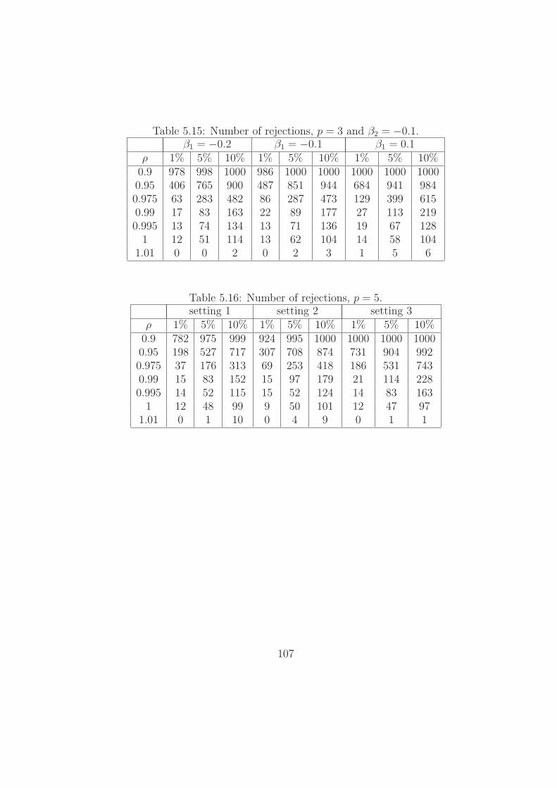
Table 5.15: Number of rejections, p = 3 and β2 = −0.1.β1 = −0.2 β1 = −0.1 β1 = 0.1

ρ 1% 5% 10% 1% 5% 10% 1% 5% 10%0.9 978 998 1000 986 1000 1000 1000 1000 10000.95 406 765 900 487 851 944 684 941 9840.975 63 283 482 86 287 473 129 399 6150.99 17 83 163 22 89 177 27 113 2190.995 13 74 134 13 71 136 19 67 128

1 12 51 114 13 62 104 14 58 1041.01 0 0 2 0 2 3 1 5 6

Table 5.16: Number of rejections, p = 5.setting 1 setting 2 setting 3

ρ 1% 5% 10% 1% 5% 10% 1% 5% 10%0.9 782 975 999 924 995 1000 1000 1000 10000.95 198 527 717 307 708 874 731 904 9920.975 37 176 313 69 253 418 186 531 7430.99 15 83 152 15 97 179 21 114 2280.995 14 52 115 15 52 124 14 83 163

1 12 48 99 9 50 101 12 47 971.01 0 1 10 0 4 9 0 1 1

107

108

Chapter 6

Engle-Granger method

In the previous chapter we derived and simulated the properties of theDickey-Fuller test. In this chapter we would like to find the properties ofthe Engle-Granger method, which we use for testing stock price data forcointegration. As explained in chapter 4 the Engle-Granger method consistsof two steps, a linear regression followed by the Dickey-Fuller test on theresiduals of this regression. The main question is, are the critical valuesof the Engle-Granger method the same as those for the Dickey-Fuller test.In the first section the critical values of Engle-Granger method are foundby simulating price processes xt and yt with random walks, then all the as-sumptions of the method are satisfied. The second section also simulatesthe critical values but now the model from section 4.2 is used for simulatingthe processes xt and yt. Then not all assumptions are completely satisfied,because xt and yt are not strictly integrated of order one. The third sectionfinds the critical values with bootstrapping from real data. In the last sec-tion we simulate cointegrated price processes xt and yt with the alternativemethod from section 4.5 and find out whether the Engle-Granger methodrecognizes them as cointegrated. The main focus of this chapter is on thecase 2 test, but we will also compare the power of this test with the case 1test.

109

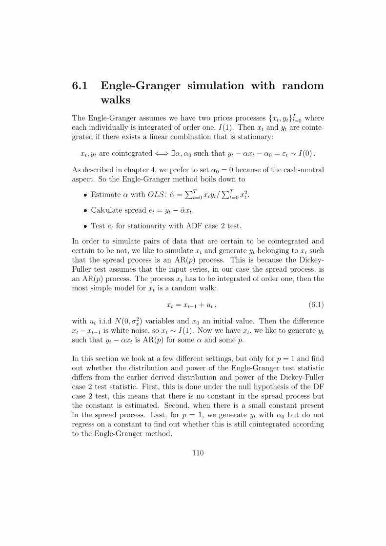
6.1 Engle-Granger simulation with random

walks

The Engle-Granger assumes we have two prices processes xt, ytTt=0 where

each individually is integrated of order one, I(1). Then xt and yt are cointe-grated if there exists a linear combination that is stationary:

xt, yt are cointegrated ⇐⇒ ∃α, α0 such that yt − αxt − α0 = εt ∼ I(0) .

As described in chapter 4, we prefer to set α0 = 0 because of the cash-neutralaspect. So the Engle-Granger method boils down to

Estimate α with OLS: α =∑T

t=0 xtyt/∑T

t=0 x2t .

Calculate spread et = yt − αxt.

Test et for stationarity with ADF case 2 test.

In order to simulate pairs of data that are certain to be cointegrated andcertain to be not, we like to simulate xt and generate yt belonging to xt suchthat the spread process is an AR(p) process. This is because the Dickey-Fuller test assumes that the input series, in our case the spread process, isan AR(p) process. The process xt has to be integrated of order one, then themost simple model for xt is a random walk:

xt = xt−1 + ut , (6.1)

with ut i.i.d N(0, σ2x) variables and x0 an initial value. Then the difference

xt− xt−1 is white noise, so xt ∼ I(1). Now we have xt, we like to generate yt

such that yt − αxt is AR(p) for some α and some p.

In this section we look at a few different settings, but only for p = 1 and findout whether the distribution and power of the Engle-Granger test statisticdiffers from the earlier derived distribution and power of the Dickey-Fullercase 2 test statistic. First, this is done under the null hypothesis of the DFcase 2 test, this means that there is no constant in the spread process butthe constant is estimated. Second, when there is a small constant presentin the spread process. Last, for p = 1, we generate yt with α0 but do notregress on a constant to find out whether this is still cointegrated accordingto the Engle-Granger method.

110

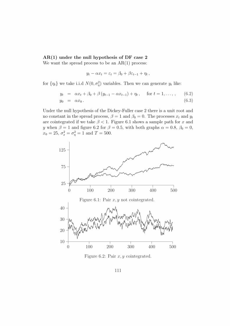
AR(1) under the null hypothesis of DF case 2We want the spread process to be an AR(1) process:

yt − αxt = εt = β0 + βεt−1 + ηt ,

for ηt we take i.i.d N(0, σ2η) variables. Then we can generate yt like:

yt = αxt + β0 + β (yt−1 − αxt−1) + ηt , for t = 1, . . . , , (6.2)

y0 = αx0 . (6.3)

Under the null hypothesis of the Dickey-Fuller case 2 there is a unit root andno constant in the spread process, β = 1 and β0 = 0. The processes xt and yt

are cointegrated if we take β < 1. Figure 6.1 shows a sample path for x andy when β = 1 and figure 6.2 for β = 0.5, with both graphs α = 0.8, β0 = 0,x0 = 25, σ2

x = σ2η = 1 and T = 500.

0 100 200 300 400 500

25

75

125

...............................................................................................................

.......................................................................................................................

.....................................................................................................................................

..........................................................................................

...............................................................................................................

.............................................................................................................................................................................................................................................................................

........................................................................

.....................................................................

..........................................................................

.......................................................................................................................

........................................................................................

......................................................................................................................................

..................................................................

..........................................................................................................................

....................................................................................................................

..............................................................................................................................................

.............................................................................................................................................................

............................................................

..........................................................................................................................................................................

................................................................................................................................

...........................................................................

.......................................................................................................................................

...................................................................................

.................................................................................................................................................

.................................................................................................

..............................................................

.............................................................................................................................................................................

Figure 6.1: Pair x, y not cointegrated.

0 100 200 300 400 50010

20

30

40

........

...................................................................................................................................................................................................................................

.......................................................................................................................................................................................................................................................................................................................................................................................................................................................................................................................................................................................................................................................................................................................................................................................................................................................................................................................................................................................................................................................................................................................................................

..................................................................................................................................................................................................................................................................................................

....................................................................................................................................................................................................................................................................................................................................................................................................................................................................................................

.....................................................................................................................................................................................................

.........................................................................................

.........................................................................................................................................................................................................................................................................................................................................................................................................................................................

.........

........................................................................................

.........................................................................................................................

............................................................................................................................................................................................................................................

..................................................................................................................................

........

........

..............................................................................................................................................................................................................................................................................................................................................................................................................................................................................................................................................................................................................................................................................................................................................................................................................................................................................................................................................................................................................................................................................................................................................................

.........

........

.........

...............................................................................................................................................................................................................................................................................................................................................................................................................................................................................................................................................................................................................................................................................................................................................................................................................................................................................................................................................................................................................................................................................................................................................................................................................................................................................................................................................................................................................................................................................................................................................................................................................................................................................................................................................................................................................................................................................................................................................................................................................

........

........

..........................................................................................................................................................................................................................................................................................................................................................................................................................

.........................................................................................................................................................................................................................................................................................................................................................................................................................................................................................................................................................................................................................................................................................................................................................................................................................................................................................................................................................................

Figure 6.2: Pair x, y cointegrated.

111

To see whether the critical values of Engle-Granger are more or less thesame as for Dickey-Fuller case 2, i.e. to see if estimating α has an affecton the critical values, we simulate a lot of paths xt and yt under the nullhypothesis and calculate the test statistic S. The procedure is:

Simulate xt.

Generate yt according to (6.2).

Calculate α.

Calculate the spread et = yt − αxt.

Calculate the spread et = yt − αxt

DF-test on the spread:Estimate β with OLS.Calculate the OLS standard error for β: σβ.

Calculate test statistic S = (β − 1)/σβ.

Repeat all this 5,000 times.

Then we estimate the density of the simulated test statistics, again with aGaussian kernel estimator. This we can compare to the density we found forthe Dickey-Fuller case 2 test in chapter 5.

Figure 6.3 shows the estimated densities for different values of α for T = 500,x0 = 25, σ2

x = σ2η = 1 and β0 = 0. The figure also shows the Dickey-Fuller

case 2 from figure 5.4. Figure 6.4 and 6.5 show estimated densities for dif-ferent values of σ2

x and σ2η respectively, for the same parameters as above

and α = 1. When the null hypothesis is completely satisfied, that is β = 1and β0 = 0, these densities look a lot like the density for the Dickey-Fullercase 2 density. So it looks like the preceding step to the DF test, namelyestimating α, does not really affect the critical values. To see if the power ofthe test is not affected by the preceding step, table 6.1 shows the number ofrejections for different values of β and α. It is clear from the table that thepower of the Engle-Granger method is not dependent of the value of α. Thistable should be compared with the columns of case 2 of table 5.9, becausethere is no constant and the initial value of the spread process is 0. We see

112

−6 −4 −2 0 20.0

0.2

0.4

..................................................................................................................................................

...........................................................................................................................................................................................................................................................................................................................................................................................................................................................................................................................................................................................................................................................................................................................................................................................................................................................

....................................................................................................................................................................................................................................................................................................................................................................................................................................................................................................................................................................................................................................................................................................................................................................................................................................................................................................................................................................

................................................

................................................................................................................................................................................................................................................................................................................................................................................................................................................................................................................................................................................................................................................................................................................................................................................................. ............. ............. ............. ............. ............. .............

............................................................................................................................................... .............

..............................................................................

..........................

.......................... ............. ............. ............. ............. ............. ............. .............

Figure 6.3: AR(1) Estimated density for EG test statistic, α = 0.1, 0.5, 1.

−6 −4 −2 0 20.0

0.2

0.4

.................................................................................................................................................................

..........................................................................................................................................................................................................................................................................................................................................................................................................................................................................................................................................................................................................................................................................................................................................................................................................................................

.................................................................................................................................................................................................................................................................................................................................................................................................................................................................................................................................................................................................................................................................................................................................................................................................................................................................................................

.............................................................................................................................................................................................................................................................................................................................................................................................................................................................................................................................................................................................................................................................................................................................................................................................................................................................................................................

................................................

................................................................................................................................................................................................................................................................................................................................................................................................................................................................................................................................................................................................................................................................................................................................................................................................. ............. ............. ............. ............. ............. .............

............................................................................................................................................... .............

..............................................................................

..........................

.......................... ............. ............. ............. ............. ............. ............. .............

Figure 6.4: AR(1) Estimated density of EG test statistic, σ2x = 0.1, 0.5, 1, 5.

−6 −4 −2 0 20.0

0.2

0.4

...................................................................................................................................................................

.........................................................................................................................................................................................................................................................................................................................................................................................................................................................................................................................................................................................................................................................................................................................................................................................................................................................................................

............................................

...............................................................................................................................................................................................................................................................................................................................................................................................................................................................................................................................................................................................................................................................................................................................................................................................

.................................................................................................................................................................................................................................................................................................................................................................................................................................................................................................................................................................................................................................................................................................................................................................................................................................................................................................

................................................

................................................................................................................................................................................................................................................................................................................................................................................................................................................................................................................................................................................................................................................................................................................................................................................................. ............. ............. ............. ............. ............. .............

............................................................................................................................................... .............

..............................................................................

..........................

.......................... ............. ............. ............. ............. ............. ............. .............

Figure 6.5: AR(1) Estimated density of EG test statistic, σ2η = 0.1, 0.5, 1, 5.

that there is practically no difference between these columns and table 6.1,which indicates that the power of the Engle-Granger method is as good asthat of the Dickey-Fuller test. The estimation of α does not have a negativeinfluence on the power of the test, which is a nice property.

113

Table 6.1: Number of rejections, AR(1) and β0 = 0α = 1 α = 0.5 α = 0.1

β 1% 5% 10% 1% 5% 10% 1% 5% 10%0.9 1000 1000 1000 1000 1000 1000 1000 1000 10000.95 722 975 1000 724 964 993 717 961 9930.975 169 485 686 164 466 683 145 469 6910.99 29 133 248 38 123 242 36 143 2540.995 14 67 149 17 75 161 18 87 163

1 14 52 105 8 51 109 10 52 1151.01 0 0 3 1 1 2 1 4 6

AR(1) with constant in spreadWhen testing for cointegration with the Engle-Granger method, we use theDickey-Fuller case 2 test which assumes there is no constant in the spreadprocess but does estimate one. It is interesting to see what happens to theproperties of the Engle-Granger method if we do include a constant, β0,in the spread process. From tables 5.11 and 5.12 we already saw that thepower of the Dickey-Fuller case 2 test was not really affected by a smallconstant, when there was no unit root. But the number of rejections whenthere was a unit root were a bit small. To be more precise, for increasingvalues of the constant the Dickey-Fuller case 2 test statistic converges to thecase 3 statistic, standard Gaussian, as explained in section 5.4. But withthe Engle-Granger method we do a preceding step, we estimate α, maybethis first step has a restraining influence on the shift. Figure 6.6 shows theestimated density of the Engle-Granger test statistic when there is a smallconstant, β0 = 0.1, in the spread process. The dashed line is the densitywhen β0 = 0. With both graphs the paths were generated with T = 500,α = 1, σx = 1, ση = 1 and β = 1. There is a shift to the right, as we couldexpect from the properties of the Dickey-Fuller test. However, the dottedline is the density when β0 = 1000, so there is a restraining influence on theshift. The Engle-Granger test statistic does not converge to the DF case 3statistic for large constants. Although this is nice, for small values of β0 westill have the same shift as for the DF case 2 statistic, so the first step inthe Engle-Granger method does not have a big influence. This can also beobserved in table 6.2, it shows the number of rejections for different values ofβ when β0 = 0.1. The power of the Engle-Granger test is rather close to the

114

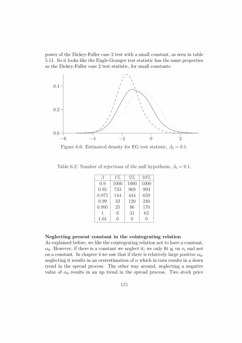
power of the Dickey-Fuller case 2 test with a small constant, as seen in table5.11. So it looks like the Engle-Granger test statistic has the same propertiesas the Dickey-Fuller case 2 test statistic, for small constants.

−6 −4 −2 0 20.0

0.2

0.4

..........................................................................................................................................................................

...................................................................................................................................................................................................................................................................................................................................................................................................................................................................................................................................................................................................................................................................................................................................................................................................................................................................................................................................................................................... ............. ............. ............. ............. .............

................................................................................................................................................................................................................

...............................................................................................................................................

..........................

.......................... ............. ............. ............. ............. ............. ............. ............. .............. . . . . . . . . . . . . . .

..................... . . . . . . .

. ................... . . . . . . . . . . . . . .

Figure 6.6: Estimated density for EG test statistic, β0 = 0.1.

Table 6.2: Number of rejections of the null hypothesis, β0 = 0.1.

β 1% 5% 10%0.9 1000 1000 10000.95 733 969 9930.975 144 444 6500.99 33 120 2400.995 25 86 170

1 6 31 621.01 0 0 0

Neglecting present constant in the cointegrating relationAs explained before, we like the cointegrating relation not to have a constant,α0. However, if there is a constant we neglect it; we only fit yt on xt and noton a constant. In chapter 4 we saw that if there is relatively large positive α0,neglecting it results in an overestimation of α which in turn results in a downtrend in the spread process. The other way around, neglecting a negativevalue of α0 results in an up trend in the spread process. Two stock price

115

processes with a trend in their spread process, do not form a good pair forour trading strategy. But for a small value of α0, there is not a big trend andthe price processes form a good pair as seen in figure 4.18. It is interestingto see how the Engle-Granger method performs if there is a small α0 butit is neglected. We can generate cointegrated data where the cointegratingrelation has a constant. We generate yt with:

yt = αxt + α0 + β0 + β (yt−1 − αxt−1) + ηt , for t = 1, . . . , T.

From this equation we can see that with this generating scheme includingα0 is a bit lame, including α0 is the same as including a larger value of β0.We have already seen what happens for larger values of β0 in figure 6.6. Butat last, we now have found a reason to use Dickey-Fuller case 2 instead ofcase 1! The power of case 1 is practically zero when there is a constant, seetable 5.13. Table 6.3 shows this is also true when we perform the precedingstep of estimating α. The table shows the number of rejections when we usecase 1 in the Engle-Granger method and the ’normal’ Engle-Granger whichuses the case 2 test. When we use the DF case 1 test in the Engle-Grangermethod instead of the case 2 test, the power is almost zero. The paths weregenerated with x0 = 25, T = 500, α = 1, σx = 1, ση = 1 and β0 = 0. Forthe value of α0 used to make table 6.3 and β < 1, we do see xt and yt asa good pair, so we like the Engle-Granger method to see them as cointegrated.

Table 6.3: Number of rejections, α0 = 1.Case 1 Case 2

β 1% 5% 10% 1% 5% 10%0.9 6 51 126 578 835 9180.95 0 0 3 196 432 5770.975 0 0 0 139 352 4920.99 0 0 0 77 256 4150.995 0 0 0 56 157 264

1 0 0 0 4 14 281.01 0 0 0 0 0 0

116

When performing the Engle-Granger test on real data we do not know ifthere is a small constant in the cointegrating relation, so from now on weonly look at the DF case 2 test. Because we use the DF case 2 test withinthe Engle-Granger method, this method makes the following assumptions:

Processes xt, yt are integrated of order one.

Spread process yt − αxt is an AR(p) process.

There is no constant in the spread process.

So far, we have seen that when all assumptions of the Engle-Granger methodare fulfilled, the Engle-Granger test statistic has the same distribution andpower properties as the DF case 2 test statistic. In other words the first stepof estimating α does not have an influence. We have seen that when thereis a constant in the spread process, so not all assumptions are fulfilled, thedistribution makes a limited shift to the right. With limited we mean thatthe Engle-Granger statistic does not converge to the DF case 3 statistic, likethe DF case 2 statistic does when there is an increasing constant. Last, wehave seen when there is a constant in the cointegrating relation it is betterto use the DF case 2 test within the Engle-Granger method instead of theDF case 1 test. In the next section we examine what happens when the priceprocesses xt and yt are not strictly integrated of order 1.

6.2 Engle-Granger simulation with stock price

model

In section 4.2 we derived a stock price model which is commonly used forthe valuation of options. This model is more realistic then the random walkfrom the preceding section. Although with this model the assumptions fromthe Engle-Granger method are not completely satisfied, it is interesting tofind out if the method performs the same.

The approach for simulating price processes xt and yt is the same as in thepreceding section, only the paths for xt are simulated with the stock pricemodel instead of random walks:

xt = xt−1 + µ δt xt−1 + σ√

δt ut xt−1 , (6.4)

117

where ut are i.i.d N(0, 1). Then xt is not exactly integrated of order 1, thereis an upward drift µ so the expectation of the differences is not constant.We look at small values of µ and for a for a finite sample size T = 500, soxt is almost integrated of order 1. By simulating a lot of paths for xt andcorresponding yt we are going to see if this effects the Engle-Granger method.

We again simulate yt such that the spread process is AR(p) and to fulfillthe remaining assumption of the method, we do not include a constant β0 inthe spread process. For p = 1 the results of the simulations are the same asin figure 6.3 through 6.5 and table 6.1, that is why they are not displayed. Itlooks like the Engle-Granger method is not sensitive for xt not being exactlyintegrated of order 1. In this section we consider the situation when thespread process is an AR(2) process.

First we need to simulate xt. Typical values of the drift parameter µ arebetween 0.01 and 0.1, and volatility σ between 0.05 and 0.5 when we measuretime in years. We like to simulate daily stock prices, so we take δt = 1/260because there are roughly 260 trading days a year. We want to generate yt

such that the spread process yt − αxt is AR(2), for some α:

yt − αxt = εt = βεt−1 + β1∆εt−1 + ηt , (6.5)

for nt we take i.i.d. N(0, σ2η) variables. Then we can generate yt like:

yt = αxt + β (yt−1 − αxt−1) + β1∆εt−1 + ηt , t = 2, . . . , T, (6.6)

y0 = αx0, y1 = αx1 ,

where we use within each step:

∆εt−1 = (yt−1 − αxt−1)− (yt−2 − αxt−2) .

We take σ2η = 0.1, because if we take the variance of η equal to 1 then yt is

much more jagged than xt and we are trying to model the price processesmore realistically. Then xt and yt are cointegrated if β < 1. Again weestimate the density of the Engle-Granger test statistic by simulating fordifferent values of α in the same way as the previous paragraph. The resultsare shown in figure 6.7 for T = 500, x0 = 25, µ = 0.05, σ = 0.20 , β1 = −0.1and of course β = 1. The density of the Engle-Granger test statistic is againcomparable with the density of the Dickey-Fuller case 2 statistic.

118

−4 −2 0 20.0

0.2

0.4

....................................................................................................................................................................................

................................................................................................................................................................................................................................................................................................................................................................................................................................................................................................................................................................................................................................................................................................................................................................................................................................................................................................................................................................................................................................................................................................................................................................................................................................................

.......................................

.............................................................................................................................................................................................................................................................................................................................................................................................................................................................................................................................................................................................................................................................................................................................................................................................................................................................................................................................................................................................................................................................................................................................................................................................................................................................

........................................

..................................................................................................................................................................................................................................................................................................................................................................................................................................................................................................................................................................................................................................................................................................................................................................................................................................................................................................................................................................................................................................................... ............. ............. ............. ............. ............. ............. .............

................................................................................................................................................................................................................ .............

..................................................................................................................................

..........................

..........................

............. ............. ............. ............. ............. ............. ............. ............. .............

Figure 6.7: AR(2) Estimated density for EG test statistic , α = 0.1, 0.5, 1.

Table 6.4 shows the number of rejections for three different values of β1.Compared to table 5.14, which shows the corresponding power of the Dickey-Fuller case 2 test, the power of the Engle-Granger method has not declined. Itseems that the Engle-Granger performs the same for data that is not exactlyintegrated of order one, as for data that is.

Table 6.4: Number of rejections, AR(2) and β0 = 0.β1 = −0.25 β1 = −0.1 β1 = 0.1

β 1% 5% 10% 1% 5% 10% 1% 5% 10%0.9 987 1000 1000 999 1000 1000 1000 1000 10000.95 477 834 945 611 925 986 825 986 9980.975 98 337 505 139 404 617 197 569 7560.99 15 98 176 24 126 234 30 150 2620.995 12 66 143 12 65 144 21 97 163

1 8 61 111 11 53 101 13 50 1041.01 1 2 5 0 2 3 1 4 4

119

6.3 Engle-Granger with bootstrapping from

real data

So far we have simulated paths xt and yt from scratch to find the criticalvalues of the Engle-Granger method. In this section we build paths xt andyt by bootstrapping from real data. The data are the ten pairs of stocks thatIMC provided. First we describe the bootstrap procedure and then we lookat some results of the ten pairs.

Bootstrap procedureAssume we have a pair that consists of two stock price processes xt and yt,for t = 0, . . . , T , which are integrated of order one. Let us assume furtherthat there exists an α such that yt − αxt follows an AR(p) process:

yt − αxt = εt = β0 + βεt−1 + β1∆εt−1 + · · ·+ βp−1∆εt−p+1 + ηt . (6.7)

The null hypothesis of no cointegration against the alternative that there iscointegration between xt and yt can be formulated as

H0 : β = 1 against H1 : β < 0 .

The first step in the bootstrap procedure is to estimate α with OLS, whichresults in α. Then we can calculate the spread process:

et = yt − αxt, t = 0, . . . , T,

this resembles the true spread process εt which is assumed to follow an AR(p)process.

In the preceding sections we knew the value of p but now do not, sincewe are working with real data. The second step is to estimate p with theinformation criteria described in chapter 3, which results in p.

The third step is to estimate the coefficients of the AR(p) model with linearregression, which results in β, β0, β1, . . . , βp−1. Then we can calculate theresiduals:

nt = et − β0 − βet−1 − β1∆et−1 − · · · − βp−1∆et−p+1, t = p, . . . , T,

120

this resembles the true residuals ηt which are assumed to be white noise.

The fourth step is to calculate the test statistic for the real data

S =β − 1

σβ

,

where σβ is the standard error of β.

Now we are ready to build a new path y∗t that belongs to the original xt.This is done in the following way:

y∗t = αxt + ε∗t , t = p, . . . , T,

where ε∗t is built under the null hypothesis, that is β = 1 and β0 = 0:

ε∗t = ε∗t−1 + β1∆ε∗t−1 + · · ·+ βp−1∆ε∗t−p+1 + η∗t ,

with η∗t is taking uniform out of nt. We initialize the new path by:

ε∗i = yi − αxi, i = 0, . . . , p− 1.

We treat the new pair xt, y∗t the same way as with the original pair xt, yt.

That is, we calculate α∗ and spread process e∗t = y∗t−α∗xt which should followan AR(p) process. Then we estimate the coefficients of this AR(p) processand calculate the test statistic S∗:

S∗ =β∗ − 1

σβ∗.

By building a lot of new paths y∗t and calculating the corresponding teststatistic S∗, we can calculate the density of these bootstrapped test statis-tics. Then we can see if the test statistic of the real pair is exceptional. Theestimated density should also give an indication for the critical values of theEngle-Granger method.

ResultsThe ten provided pairs are named pair I, pair II,..., pair X. We start with apair for which all three information criteria indicate that the spread processis AR(1), pair II. By spread process we mean the residuals from the first

121

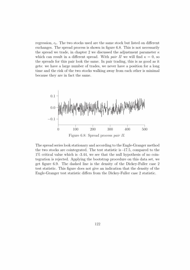
regression, et. The two stocks used are the same stock but listed on differentexchanges. The spread process is shown in figure 6.8. This is not necessarilythe spread we trade, in chapter 2 we discussed the adjustment parameter κwhich can result in a different spread. With pair II we will find κ = 0, sothe spreads for this pair look the same. In pair trading, this is as good as itgets: we have a large number of trades, we never have a position for a longtime and the risk of the two stocks walking away from each other is minimalbecause they are in fact the same.

0 100 200 300 400 500

−0.1

0.0

0.1

.........................................................................................................................................................................................................................................................................................................................................................................................................................................................................................................................................................................................................................................................................................................................................................................................................................................................................................................................................................................................................................................................................................................................................................................................................................................................................................................................................................................................................................................................................................................................................................................................................................................................................................................................................................................................................................................................................................................................................................................................................................................................................................................................................................................................................................................................................................................................................................................................................................................................................................................................................................................................................................................................................................................................................................................................................................................................................................................................................................................................................................................................................................................................................................................................................................................................................................................................................................................................................................................................................................................................................................................................................................................................................................................................................................................................................................................................................................................................................................................................................................................................................................................................................................................................................................................................................................................................................................................................................................................................................................................................................................................................................................................................................................................................................................................................................................................................................................................................................................................................................................................................................................................................................................................................................................................................................................................................................................................................................................................................................................................................................................................................................................................................................................................................................................................................................................................................................................................................................................................................................................................................................................................................................................................................................................................................................................................................................................................................................................................................................................................................................................................................................................................................................................................................................................................................................................................................................................................................................................................................................................................................................................................................................................................................................................................................................................................................................................................................................................................................................................................................................................................................................................................................................................................................................................................................................................................................................................................................................................................................................................................................................................................................................................................................................................................................................................................................................................................................................................................................................................................................................................................................................................................................................................................................................................................................................................................................................................................................................................................................................................................................................................................................................................................................................................................................................................................................................................................................................................................................................................................................................................................................................................................................................................................................................................................................................................................................................................................................................................................................................................................................................................................................................................................................................................................................................................................................................................................................................................................................................................................................................................................................................................................................................................................................................................................................................................................................................................................................................................................................................................................................................................................................................................................................................................................................................................................................................................................................................................................................................................................................................................................................................................................................................................................................................................................................................................................................................................................................................................................................................................................................................................................................................................................................................................................................................................................................................................................................................................................................................................................................................................................................................................................................................................................................................................................................................................................................................................................................................................................................................................................................................................................................................................................................................................................................................................................................................................................................................................................................................................................................................................................................................................................................................................................................................................................................................................................................................................................................................................................................................................................................................................................................................................................................................................................................................................................................................................................................................................................................................................................................................................................................................................................................................................................................

Figure 6.8: Spread process pair II.

The spread series look stationary and according to the Engle-Granger methodthe two stocks are cointegrated. The test statistic is -17.5, compared to the1% critical value which is -3.44, we see that the null hypothesis of no coin-tegration is rejected. Applying the bootstrap procedure on this data set, weget figure 6.9. The dashed line is the density of the Dickey-Fuller case 2test statistic. This figure does not give an indication that the density of theEngle-Granger test statistic differs from the Dickey-Fuller case 2 statistic.

122

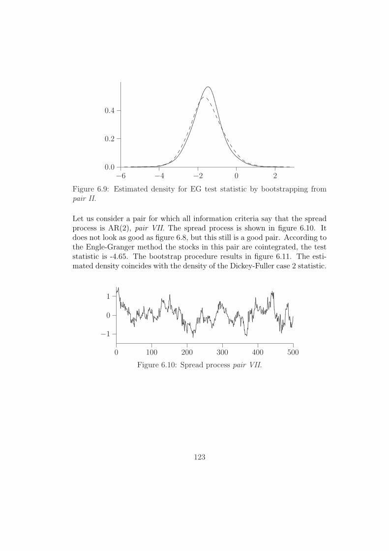
−6 −4 −2 0 20.0

0.2

0.4

.......................................................................................................................................................................

............................................................................................................................................................................................................................................................................................................................................................................................................................................................................................................................................................................................................................................................................................................................................................................................................................................................................................................................... ............. ............. ............. ............. ............. .............

............................................................................................................................................................ .............

...........................................................................................

..........................

.......................... ............. ............. ............. ............. ............. ............. .............

Figure 6.9: Estimated density for EG test statistic by bootstrapping frompair II.

Let us consider a pair for which all information criteria say that the spreadprocess is AR(2), pair VII. The spread process is shown in figure 6.10. Itdoes not look as good as figure 6.8, but this still is a good pair. According tothe Engle-Granger method the stocks in this pair are cointegrated, the teststatistic is -4.65. The bootstrap procedure results in figure 6.11. The esti-mated density coincides with the density of the Dickey-Fuller case 2 statistic.

0 100 200 300 400 500

−1

0

1..................................................................................................................................................................................................................................................................................................................................................................................................................................................................................................................................................................................................................................................................................................................................................................................................................................................................................................................................................................................................................................................................................................................................................................................................

..................................................................................................................................................................................................................................................................................

........

.............................................................................................................................................................................................................................................................................................................................................................................................................................................................

........

........

........

........

..........................................................................................................................................................................................................................................................................................................................................................................................................................................................................................................................................................................................................................................................................................................................................................................................................................................................................................................................

......................................................................................................................................................................................................................................................................................................................................................

........

...........................................................................................................................................................................................................................................................................................................................................................................................................................................................................................................................................................................

.........

........

...........................................................................................................................................................................................................................................................................................................................................................................................................................................................................................................................................................................................................................................................................................................................................................................................................................................................................................................................................................................................................................................................................................................................................................................................................................................................................................................................................................................................................................................................................................................................................................................................................................................................................................................................................................................................................................................................................................................................................................

Figure 6.10: Spread process pair VII.

123

−6 −4 −2 0 20.0

0.2

0.4

....................................................................................................................................................................................................................

................................................................................................................................................................................................................................................................................................................................................................................................................................................................................................................................................................................................................................................................................................................................................................................................................................................... ............. ............. ............. ............. ............. .............

............................................................................................................................................................ .............

...........................................................................................

..........................

.......................... ............. ............. ............. ............. ............. ............. .............

Figure 6.11: Estimated density for EG test statistic by bootstrapping frompair VII.

Let us consider a pair for which all information criteria indicate that thespread process is AR(3), pair VI. The spread process is shown in figure 6.12.This looks a lot less interesting than the previous figure: initially the spreadis below zero for a long time and at the end the spread is above zero for along time. This shows that trading the spread would have resulted in only afew trades and we would have had the same position for a long time. But thisis not necessarily the spread we trade as stated, in the next chapter we willsee the spread we would have really traded. According to the Engle-Grangermethod the stocks in this pair are not cointegrated, the test statistic is -2.23. The null hypothesis of no cointegration is not even rejected at the 10%level. The bootstrap procedure results in figure 6.13. The estimated densityis a bit bumpy but still coincides with the density of the Dickey-Fuller case2 statistic. Even when the real data is not cointegrated, according to theEngle-Granger method, the bootstrap procedure finds nearly the same den-sity as the density of the Dickey-Fuller test statistic.

So far we have seen pairs for which all information criteria find the samesmall value of p. IMC also provided a pair for which the information criteriafind p to be very large, pair V. As described in chapter 3 we fit an AR(k)model, for k = 1, . . . , K, on the data and see for which k the criteria have tolowest values. For this pair, even if we set K = 100 the criteria have to lowestvalue for p = K. This indicates that the spread process does not follow anAR(p) model. The spread process is shown in figure 6.14. It is obvious that

124

0 100 200 300 400 500

−2

0

2......................................

.........

..........................................................................................................................................................................................................................................

........................................................................................................................................................................................................................................................................................................................................................................................................................................................................................................................................................................................

............................................................................................................................................................................................................................................................................................................................................................................................................................................................................................................................................................................................................................................................................................................................................................................................................................................................................................................................................................................................................................................................................................................................................................................................................

.......................................................................................................................................................................................................................................................................................................................................................................................................................................................................................................................................................................................................................................................................................................................................................................................................

........

...................................................................................................................................................................................................................................................................................................................................................................................................................................................................................................................................................................................................................................................................................................................................................................................................................................................................................................................................................................................................................................................................................................................................................................................................................................................................................................................................................................

.................................................................................................................................................................................................................................................................................................................................................................................................................................................................................................................................

........

..................................................................................................................................................................................................................................................................................................................................................................................................................................................

Figure 6.12: Spread process pair VI.

−6 −4 −2 0 20.0

0.2

0.4

...............................................................................................................................

.................................................................................................................................................................................................................................................................................................................................................................................................................................................................................................................................................................................................................................................................................................................................................................................................................. ............. ............. ............. ............. ............. .............

............................................................................................................................................................ .............

...........................................................................................

..........................

.......................... ............. ............. ............. ............. ............. ............. .............

Figure 6.13: Estimated density for EG test statistic by bootstrapping frompair VI.

this ’pair’ is not suitable for pair trading. The Engle-Granger method doesnot reject the null hypothesis of no cointegration because the test statistic is-1.04 when p = 10 and 0.63 if p = 100. To apply to bootstrap procedure, weset p = 10. The result is shown in figure 6.15, which coincides surprisinglywell with the density of the Dickey-Fuller case 2 test statistic.

We examine these and the remaining pairs further in chapter 7. In thischapter, we have seen no reason to assume that the test statistic of theEngle-Granger has a different distribution than the Dickey-Fuller case 2 teststatistic. The power of the two tests are also comparable. To find out if theEngle-Granger method is also ’robust’, we apply the method on generateddata which do not fulfill the null hypothesis.

125

0 100 200 300 400 500

−100

0

100

200

........................................................................................................................................................................

............................................................................................................................

.......................................................................................................................................................................................................................................................................................................

...............................................................................................

.....................................................................................................................................................................................................

....................................................................................................................................................................................................................

..........................................................................................

.......................................................................................................................

.....................................................................................................................................................................

..................................................................................................................................................................................................................................

........

........

........

........

........

........

........

........

........

..................................................................................................................................................................................................................................................................................................................................................................................................................................

......................................................................................................

...................................................................................................................................................................................................................................................................................................................................................................................................................................................................................................................

........

........

...............................................................

.......................................................................................................

...............................................................................................................................................................................................................................................................................................................................................

Figure 6.14: Spread process pair V.

−6 −4 −2 0 20.0

0.2

0.4

........................................................................................................................................................

....................................................................................................................................................................................................................................................................................................................................................................................................................................................................................................................................................................................................................................................................................................................................................................................................................... ............. ............. ............. ............. ............. .............

............................................................................................................................................................ .............

...........................................................................................

..........................

.......................... ............. ............. ............. ............. ............. ............. .............

Figure 6.15: Estimated density for EG test statistic by bootstrapping frompair V.

6.4 Engle-Granger simulation with alterna-

tive method

In section 4.5 we found a method for generating cointegrated data which donot satisfy the assumptions of the Engle-Granger method. The generateddata is integrated of order one, but the spread process is not likely to followan AR(p) process. It is interesting to find out if the Engle-Granger methodis robust enough to see this data as cointegrated.

126

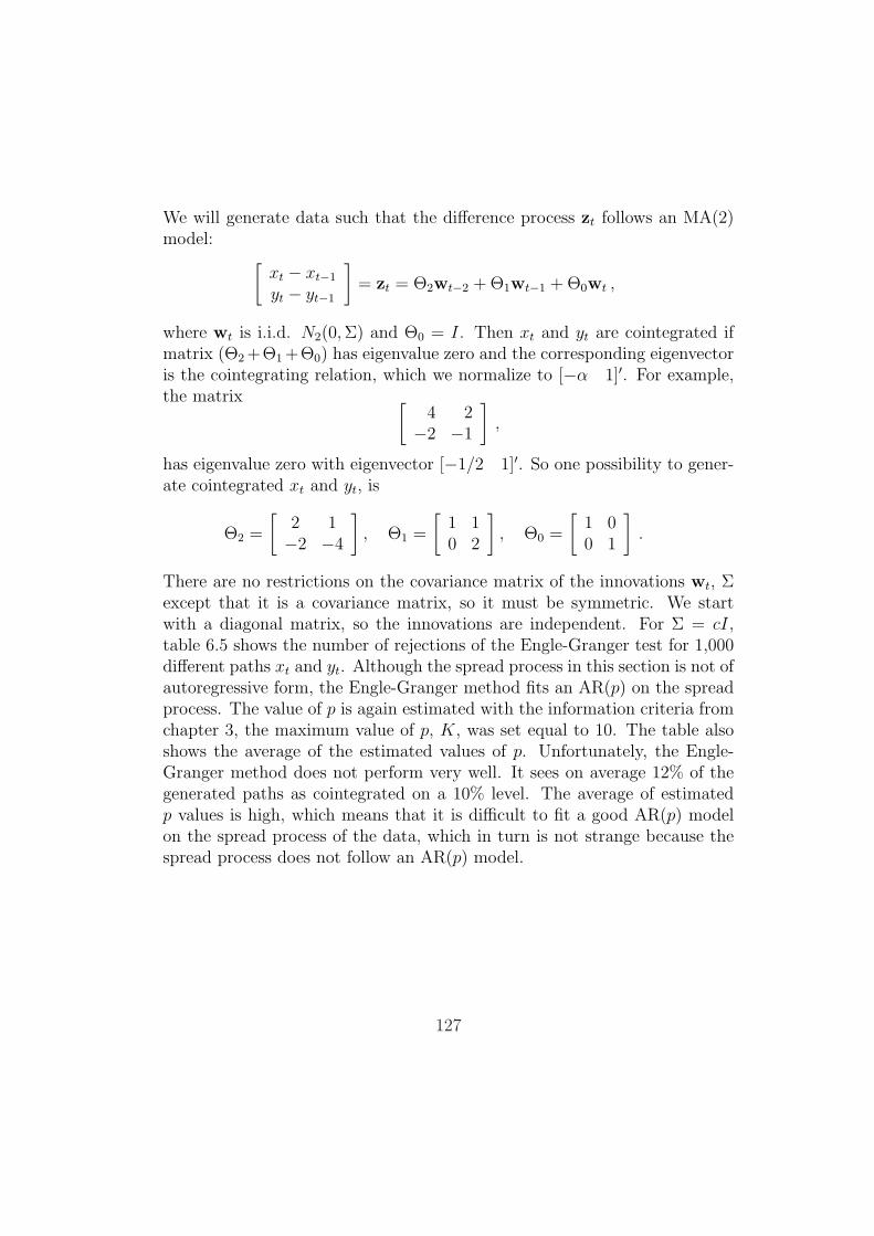
We will generate data such that the difference process zt follows an MA(2)model:

[xt − xt−1

yt − yt−1

]= zt = Θ2wt−2 + Θ1wt−1 + Θ0wt ,

where wt is i.i.d. N2(0, Σ) and Θ0 = I. Then xt and yt are cointegrated ifmatrix (Θ2 +Θ1 +Θ0) has eigenvalue zero and the corresponding eigenvectoris the cointegrating relation, which we normalize to [−α 1]′. For example,the matrix [

4 2−2 −1

],

has eigenvalue zero with eigenvector [−1/2 1]′. So one possibility to gener-ate cointegrated xt and yt, is

Θ2 =

[2 1−2 −4

], Θ1 =

[1 10 2

], Θ0 =

[1 00 1

].

There are no restrictions on the covariance matrix of the innovations wt, Σexcept that it is a covariance matrix, so it must be symmetric. We startwith a diagonal matrix, so the innovations are independent. For Σ = cI,table 6.5 shows the number of rejections of the Engle-Granger test for 1,000different paths xt and yt. Although the spread process in this section is not ofautoregressive form, the Engle-Granger method fits an AR(p) on the spreadprocess. The value of p is again estimated with the information criteria fromchapter 3, the maximum value of p, K, was set equal to 10. The table alsoshows the average of the estimated values of p. Unfortunately, the Engle-Granger method does not perform very well. It sees on average 12% of thegenerated paths as cointegrated on a 10% level. The average of estimatedp values is high, which means that it is difficult to fit a good AR(p) modelon the spread process of the data, which in turn is not strange because thespread process does not follow an AR(p) model.

127

Table 6.5: Number of rejections, Σ = cI.c 1% 5% 10% p2 47 89 147 9.91 25 77 125 9.6

0.5 24 61 116 9.10.1 11 49 102 7.6

Consider the situation when the innovations are correlated, we take Σ of theform:

A =

[1 ρρ 1

].

Table 6.6 shows the number of rejections of the Engle-Granger test for differ-ent values of ρ. Even for ρ = 1 the Engle-Granger method does not performwell.

Table 6.6: Number of rejections, Σ = Aρ 1% 5% 10% p1 34 86 140 9.8

0.5 31 67 134 9.7

To see what happens, figure 6.16 shows the spread process of a realizationxt and yt. This does not look stationary, there seems to be a trend in thespread process. This could mean that with this setting there a is a constantin the cointegrating relation, α0. Figure 6.17 shows the spread process if weregress the same realization of yt on the same xt and a constant.

It is clear that there is a constant, α0, in the cointegrating relation. Ne-glecting the constant, results in a spread process which is not stationary.That is why the Engle-Granger method does not reject the null hypothesisof no cointegration. Table 6.7 shows the number of rejection when we donot neglect α0 and take Σ = cI. The maximum value of p is set to 5 inthe remainder of this section, to reduce computation time. It is clear thatthe Engle-Granger method performs very well, almost every path is seen ascointegrated (which is true).

128

0 100 200 300 400 5000

50

100

150

200

250

.................................................................................................................................................................................................................................................................................................................................................................................................................................................

.........

........

.........

........

........................................................................................................................................................................................................................................................................................................................................................................................................

..................................................................................................................................................................................................................................................................................................

..................................................................................................................................................................................................................................................................................................................................................................................

......................................................................................................................................................................................................................................................................

..........................................................................................................................................................................................

........

....................................................................................................................................................................................................................................................................................................................................................................................................................................................................................................................................................................................................................................................................................................................................................................................................................................................................................................................................................................................................................................................................................................................................................................................................................................................................................................................................................................................................

........

.........

........

.......................................................................................................................................................................................

..............................................................................................................................................................................................................................................................................................................................................................................................................................................................................................................................................................................................................................................................................

Figure 6.16: Realization spread setting 1, ρ = 0.5.

0 100 200 300 400 500

−10

−5

0

5

10

........

........

........

........

..........................................................................................................................................................................................................................................................................................................................................................................................................................................................................................................................................................................................................................................................................................................................................................................................................................................................................................................................................................................................................................................................................................................................................................................................................................................................................................................................................................................................................................................................................................................................................................................................................................................................................................................................................................................................................................................................................................................................................................................................................................................................................................................................................................................................................................................................................................................................................................................................................................................................................................................................................................................................................................................................................................................................................................................................................................................................................................................................................................................................................................................................................................................................................................................................................................................................................................................................................................................................................................................................................................................................................................................................................................................................................................................................................................................................................................................................................................................................................................................................................................................................................................................................................................................................................................................................................................................................................................................................................................................................................................................................................................................................................................................................................................................................................................................................................................................................................................................................................................................................................................................................................................................................................................................................................................................................................................................................................................................................................................................................................................................................................................................................................................................................................................................................................................................................................................................................................................................................................................................................................................................................................................................................................................................................................................................................................................................................................................................................................................................................................................................................................................................................................................................................................................................................................................................................................................................................................................................................................................................................................................................................................................................................................................................................................................................................................................................................................................................................................................................................................................................................................................................................................................................................................................................................................................................................................................................................................................................................................................................................................................................................................................................................................................................................................................................................................................................................................................................................................................................................................................................................................................................................................................................................................................................................................................................................................................................................................................................................................................................................................................................................................................................................................................................................................................................................................................................................................................................................................................................................................................................................................................................................................................................................................................................................................................................................................................................................................................................................................................................................................................................................................................................................................................................................................................................................................................................................................................................................................................................................................................................................................................................................................................................................................................................................................................................................................................................................................................................................................................................................................................................................................................................................................................................................................................................................................................................................................................................................................................................................................................................................................................................................................................................................................................................................................................................................................................................................................................................................................................................................................................................................................................................................................................................................................................................................................................................................................................................................................................................................................................................................................................................................................................................................................................................................................................................................................................................................................................................................................................................................................................................................................................................................................................................................................................................................................................................................................................................................................................................................................................................................................................................................................................................................................................................................................................................................................................................................................................................................................................................................................................................................................................................................................................................................................................................................................................................................................................................................................................................................................................................................................................................................................................................................................................................................................................................................................................................................................................................................................................................................................................................................................................................................................................................................................................................................................................................................................................................................................................................................................................................................................................................................................................................................................................................................................................................................................................................................................................................................................................................................................................................................................................................................................................................................................................................................................................................................................................................................................................................................................................................................................................................................................................................................................................................................................................................................................................................................................................................................................................................................................................................................................................................................................................................................................................................................................................................................................................................................................................................................................................................................................................................................................................................................................................................................................................................................................................................................................................................................................................................................................................................................................................................................................................................................................................................................................................................................................................................................................................................................................................................................................................................................................................................................................................................................................................................................................................................................................................................................................................................................................................................................................................................................................................................................................................................................................................................................................................................................................................................................................................................................................................................................................................................................................................................................................................................................................................................................................................................................................................................................................................................................................................................................................................................................................................................................................................................................................................................................................................................................................................................................................................................................................................................................................................................................................................................................................................................................................................................................................................................................................................................................................................................................................

Figure 6.17: Realization spread setting 1, with α0.

Table 6.7: Number of rejections, with α0 and Σ = cI.c 1% 5% 10% p2 1000 1000 1000 4.71 1000 1000 1000 4.5

0.5 999 1000 1000 4.30.1 1000 1000 1000 3.5

129

So far, we have generated cointegrated data but not in the way we wantit to be cointegrated, which is data with a small or no constant α0. We lookat a different setting of parameters:

Θ2 =

[1 −1−1 0

], Θ1 =

[ −1 22 0

], Θ0 =

[1 00 1

].

The matrix (Θ2 + Θ1 + Θ0) has eigenvalue zero with eigenvector [−1 1]′.Figure 6.18 shows a realization of the spread process, when yt is only re-gressed on xt and not on a constant. In other words, we neglect a possibleα0.

0 100 200 300 400 500−5

0

5

10

........

........

........

........

........

......................................................................................................................................................................................................................................................................................................................................................................................................................................................................................................................................................................................................................................................................................................................................................................................................................................................................................................................................................................................................................................................................................................................................................................................................................................................................................................................................................................................................................................................................................................................................................................................................................................................................................................................................................................................................................................................................................................................................................................................................................................................................................................................................................................................................................................................................................................................................................................................................................................................................................................................................................................................................................................................................................................................................................................................................................................................................................................................................................................................................................................................................................................................................................................................................................................................................................................................................................................................................................................................................................................................................................................................................................................................................................................................................................................................................................................................................................................................................................................................................................................................................................................................................................................................................................................................................................................................................................................................................................................................................................................................................................................................................................................................................................................................................................................................................................................................................................................................................................................................................................................................................................................................................................................................................................................................................................................................................................................................................................................................................................................................................................................................................................................................................................................................................................................................................................................................................................................................................................................................................................................................................................................................................................................................................................................................................................................................................................................................................................................................................................................................................................................................................................................................................................................................................................................................................................................................................................................................................................................................................................................................................................................................................................................................................................................................................................................................................................................................................................................................................................................................................................................................................................................................................................................................................................................................................................................................................................................................................................................................................................................................................................................................................................................................................................................................................................................................................................................................................................................................................................................................................................................................................................................................................................................................................................................................................................................................................................................................................................................................................................................................................................................................................................................................................................................................................................................................................................................................................................................................................................................................................................................................................................................................................................................................................................................................................................................................................................................................................................................................................................................................................................................................................................................................................................................................................................................................................................................................................................................................................................................................................................................................................................................................................................................................................................................................................................................................................................................................................................................................................................................................................................................................................................................................................................................................................................................................................................................................................................................................................................................................................................................................................................................................................................................................................................................................................................................................................................................................................................................................................................................................................................................................................................................................................................................................................................................................................................................................................................................................................................................................................................................................................................................................................................................................................................................................................................................................................................................................................................................................................................................................................................................................................................................................................................................................................................................................................................................................................................................................................................................................................................................................................................................................................................................................................................................................................................................................................................................................................................................................................................................................................................................................................................................................................................................................................................................................................................................................................................................................................................................................................................................................................................................................................................................................................................................................................................................................................................................................................................................................................................................................................................................................................................................................................................................................................................................................................................................................................................................................................................................................................................................................................................................................................................................................................................................................................................................................................................................................................................................................................................................................................................................................................................................................................................................................................................................................................................................................................................................................................................................................................................................................................................................................................................................................................................................................................................................................................................................................................................................................................................................................................................................................................................................................................................................................................................................................................................................................................................................................................................................................................................................................................................................................................................................................................................................................................................................................................................................................................................................................................................................................................................................................................................................................................................................................................................................................................................................................................................................................................................................................................................................................................................................................................................................................................................................................................................................................................................................................................................................................................................................................................................................................................................................................................................................................................................................................................................................................................................................................................................................................................................................................................................................................................................................................................................................................................................................................................................................................................................................................................................................................................................................................................................................................................................................................................................................................................................................................................................................................................................................................................................................................................................................................................................................................................................................................................................................................................................................................................................................................................................................................................................................................................................................................................................................................................................................................................................................................................................................................................................................................................................................................................................................................................................................................................................................................................................................................................................................................................................................................................................................................................................................................................................................................................................................................................................................................................................................................................................................................................................................................................................................................................................................................................................................................................................................................................................................................................................................................................................................................................................

Figure 6.18: Realization spread setting 2, ρ = 0.5.

Neglecting α0 with this setting is no problem, the spread process seems tobe stationary. We wish Engle-Granger method to see the corresponding xt

and yt as cointegrated. Table 6.8 and 6.9 show the number of rejections forΣ = cI and Σ = A respectively. The power of the Engle-Granger test isgood, almost every time the null is rejected.

The Engle-Granger method performs very well, even when the spread processdoes not follow an AR(p) model, the test behaves exactly how we want it. Ifthere is a large constant α0 in the cointegrating relation, it does not rejectthe null hypothesis of no cointegration. Although the data is cointegrated, itis not cointegrated the way we want it, that is with a small or no α0. If thereis a small or no constant in the cointegration relation, the test has rejectedthe null hypothesis almost every time.

130

Table 6.8: Number of rejections, setting 2 Σ = cI.c 1% 5% 10% p2 946 980 992 4.831 974 988 997 4.75

0.5 981 992 995 4.600.1 995 998 999 3.95

Table 6.9: Number of rejections, setting 2 Σ = A.ρ 1% 5% 10% p1 991 996 999 4.7

0.5 970 991 996 4.6

131

132

Chapter 7

Results

In this chapter the results for the ten pairs IMC provided are discussed. Tobe clear, IMC provided 2 years of historical closing prices for each stock ofthe ten pairs. According to IMC, among these ten are some very good pairswhich means they make high profits. Some are losing money and some aremediocre. In the first section we apply the trading strategy to the historicaldata to see which pairs would have been profitable and put the pairs in orderof profitability. We like to see if the stocks in a profitable pair are cointe-grated, and if the stocks in a pair that loses money are not cointegrated. Inother words if profitable and cointegration coincides. We apply two differentcointegration test, the Engle-Granger and the Johansen method, but first wewill examine in the second section if the assumption of the price processesbeing integrated of order 1 is fulfilled. In the third and fourth section the re-sults for respectively the Engle-Granger and the Johansen method are stated,the pairs are put in order of the levels of rejection of the cointegration tests.

7.1 Results trading strategy

The 10 pairs are named, pair I, pair II,..., pair X. In chapter 2 the tradingstrategy was explained. For each pair, we need the first half of observationsto determine the parameters of the strategy and we apply the strategy tothe second half. In order to compare the results we trade the same amountof money with each pair. With each trade we buy one stock for the amountof ¿ 10,000 and sell the other for roughly the same amount. The sell tradeis not exactly ¿ 10,000 because of the positive or negative ’investment’ of

133

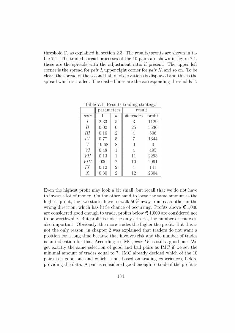
threshold Γ, as explained in section 2.3. The results/profits are shown in ta-ble 7.1. The traded spread processes of the 10 pairs are shown in figure 7.1,these are the spreads with the adjustment ratio if present. The upper leftcorner is the spread for pair I, upper right corner for pair II, and so on. To beclear, the spread of the second half of observations is displayed and this is thespread which is traded. The dashed lines are the corresponding thresholds Γ.

Table 7.1: Results trading strategy.parameters result

pair Γ κ # trades profitI 2.33 5 3 1129II 0.02 0 25 5536III 0.16 2 4 506IV 0.77 5 7 1344V 19.68 8 0 0VI 0.48 1 4 495VII 0.13 1 11 2293VIII 030 2 10 2091IX 0.12 2 4 141X 0.30 2 12 2304

Even the highest profit may look a bit small, but recall that we do not haveto invest a lot of money. On the other hand to loose the same amount as thehighest profit, the two stocks have to walk 50% away from each other in thewrong direction, which has little chance of occurring. Profits above ¿ 1,000are considered good enough to trade, profits below ¿ 1,000 are considered notto be worthwhile. But profit is not the only criteria, the number of trades isalso important. Obviously, the more trades the higher the profit. But this isnot the only reason, in chapter 2 was explained that traders do not want aposition for a long time because that involves risk and the number of tradesis an indication for this. According to IMC, pair IV is still a good one. Weget exactly the same selection of good and bad pairs as IMC if we set theminimal amount of trades equal to 7. IMC already decided which of the 10pairs is a good one and which is not based on trading experiences, beforeproviding the data. A pair is considered good enough to trade if the profit is

134

300 400 500

−5

0

5

..............................................................................................................................................................................................................................................................................................................................................................................................................................................................................................................................................................................................................................................................................................................................................................................................................................................................................................................................................................................................................................................................................................................................................................................................................................................................................................................................................................................................................................................................................................................................................................................................................................................................................................................................................................................................................................................................................................................................................................................................................................................................

......................................................................................................................................................................................................................................................................................................................................................................................................................................................................................................................................................................................................................................................................................................................................................................................................................................................................................................................................................................................................................................................................................................................

............. ............. ............. ............. ............. ............. ............. ............. ............. ............. ............. ............. ............. ...

............. ............. ............. ............. ............. ............. ............. ............. ............. ............. ............. ............. ............. ...

300 400 500

−0.1

0.0

0.1

...............................................................................................................................................................................................................................................................................................................................................................................................................................................................................................................................................................................................................................................................................................................................................................................................................................................................................................................................................................................................................................................................................................................................................................................................................................................................................................................................................................................................................................................................................................................................................................................................................................................................................................................................................................................................................................................................................................................................................................................................................................................................................................................................................................................................................................................................................................................................................................................................................................................................................................................................................................................................................................................................................................................................................................................................................................................................................................................................................................................................................................................................................................................................................................................................................................................................................................................................................................................................................................................................................................................................................................................................................................................................................................................................................................................................................................................................................................................................................................................................................................................................................................................................................................................................................................................................................................................................................................................................................................................................................................................................................................................................................................................................................................................................................................................................................................................................................................................................................................................................................................................................................................................................................................................................................................................................................................................................................................................................................................................................................................................................................................................................................................................................................................................

............. ............. ............. ............. ............. ............. ............. ............. ............. ............. ............. ............. ............. ....

............. ............. ............. ............. ............. ............. ............. ............. ............. ............. ............. ............. ............. ....

300 400 500

−1

0

1......................................................................................................................................................................

.............................................................................................................................

........................................................................................................................................................................................

............................................................................................

........................................................................................................................................................................................................................................................................................................................................................................................................................................................................................................................

.....................................................................................................................................................................

.............................................................................................................................................................................................................................................................

......................................................................................................................................................................................................................................................................................

............. ............. ............. ............. ............. ............. ............. ............. ............. ............. ............. ............. ............. ....

............. ............. ............. ............. ............. ............. ............. ............. ............. ............. ............. ............. ............. ....

300 400 500

−2

0

2

...................................................................................................................................................................................................................................................................................................................................................................................................................................................................................................................................................................................................................................................

.........

.........

........

...........................................................................................................................................................................................................................................................................................

.........

........

........

...............................................................................................................................................................................................................................................................................................................................................................................................................................................................................................................................................................................................................................................................................................................................................................................

..................................................................................................................................................................................................................................................................................................................................................................................................................................................................................................................................................................................................................................................................................

.........

.................................................................................................................................................................................................................................................................................................................................

............. ............. ............. ............. ............. ............. ............. ............. ............. ............. ............. ............. ............. ....

............. ............. ............. ............. ............. ............. ............. ............. ............. ............. ............. ............. ............. ....

300 400 500

−10

0

10 ....................................................................................................................................................................................................................................................

............................................................................................................................................................................................................................................................................................................................................................................................................................................................................................................................................................................................................................................................................................................................................................................................................................................................................................................................................................................................................................................................................................................................................................................................................................................................................................................................................................................................................................................................................................................................................................................................................................................................................................................................................................................................................................................................................................................................................................................................................................................................................................................................................................................................................................................................................................................................................................................................................................................................................................................................................................................................................................................................................................................................................................................................................................................................................................................................................................................................................................................................................................................................................................................................................................................................................................................................................................................................................................................................................................................................................................................................................................................................................................................................................................................................................................................................................................................................................................................................................................................................................................................................................................................................................................................................................................................................................................

300 400 500

−1

0

1...........................................................................................................................................................................................................................................................................................................................................................................................................................................................................................................................................................................................................................................................................................................................................................................................................................................................................................................................................................................................................................................................................................................................................................................................................................................................................................................................................................................................................................................................................................................................................................................................................................................................................................................................................................................................................................................................................................................................................................................................................................................................................................................................................................................................................................................................................................................................................................................................................................................................................................................................................................................................................................................................................................................................................................................................................................................................................................................................................................................................................................................................................................................................................................................................................................................................................................................................................................................................................................................................................................................................................................

........

..................................................................................................................................................................................................................................................................................................................................................................................................................................................................................................................................................................................................................................................................................................................................................................................................................................................................................................................................................................................

............. ............. ............. ............. ............. ............. ............. ............. ............. ............. ............. ............. ............. ....

............. ............. ............. ............. ............. ............. ............. ............. ............. ............. ............. ............. ............. ....

300 400 500−1

0

1

.............................................................................................................................................................................................................

........

........................................................................................................................................................................................................................................................................................................................................................................................................................................................................................................................................................................................................................................................................................................................................................................................

........

........

........

...........................................................................................................................................................................................................................................................................................................................................................................................................................................................................................................................................................................................................................................................................................................................................................................................................................................................................................................................................................................................................................................................................................................................................................................................................................................................................................................................................................................................................................

..........................................................................................................................................................................................................................................................................................................................................................................................................................................................................................................

............. ............. ............. ............. ............. ............. ............. ............. ............. ............. ............. ............. ............. ....

............. ............. ............. ............. ............. ............. ............. ............. ............. ............. ............. ............. ............. ....

300 400 500−1

0

1

.......................................................................................................................................................................................................................................................................................................................................................................................................................................................................................................................................................................................................................................................

........

................................................................................................................................................................................................................................................................................................................................................................................................................................................................................................................................................................................................................................................................................................................................................................................................................................................................................................................................................................................................................................................................................................................................................................................................................................................................................................................................................................................................................................................................................................................................................................................................................................................................................................................

........

........

........

.............................................................................................................................................................................................................................................................................

........

........

.........

.........

.....................................................................................................................

............. ............. ............. ............. ............. ............. ............. ............. ............. ............. ............. ............. ............. ....

............. ............. ............. ............. ............. ............. ............. ............. ............. ............. ............. ............. ............. ....

300 400 500

−0.5

0.0

0.5....................................................................................................................................................................

................................................................................................................................................................................................

........................................................................................

................................................................................................................................................................................................................

........

........

........

..........................................................................................................................................................................................................................................................................................................................................................................................................................................................................................................................................................................................................................................................................................................................................................................................................................................................................................................................

.........

........

.........

.........

........

..........................................................................................................................

..............................................................................................

............. ............. ............. ............. ............. ............. ............. ............. ............. ............. ............. ............. ............. ....

............. ............. ............. ............. ............. ............. ............. ............. ............. ............. ............. ............. ............. ....

300 400 500

−4

−2

0

2

.......................................................................................................................................

........

..............................................................................................................................................................................................................................................................................................................................................................................................................................................................................................................................................................................................................................................................................................................................

.........................................................................................................................................................................................................................................................................................................

.........

.....................................................................................................................................................................................................................................................................................................................................................................................................................................................................................................................................................................................................................................................................................................................................................................................................................................................................................................................................................................................................................................................................................................................................................................................................................................................................................................................................................................................................................................................................................................................................................................................................................................................................

............. ............. ............. ............. ............. ............. ............. ............. ............. ............. ............. ............. ............. ....

............. ............. ............. ............. ............. ............. ............. ............. ............. ............. ............. ............. ............. ....

Figure 7.1: Traded spreads.

135

above ¿ 1,000 and the number of trades is no less than 7, otherwise the pairis considered not to be worthwhile. The ordering of the 10 pairs based purelyon the results from the trading strategy, where the first five are consideredgood or good enough, the remaining five are not, is:

1 pair II2 pair X3 pair VII4 pair VIII5 pair IV6 pair I7 pair III8 pair VI9 pair IX10 pair V

We briefly discuss the spreads from figure 7.1. The spread for pair I is rarelyhitting its threshold Γ although the adjustment parameter κ is large. Thespread for pair II looks good, but it could be better if we had used κ = 1.After t = 425 the spread is a relatively long time below +Γ, with κ = 1 wewould have made a profit of ¿ 6721 in 36 trades. The spreads for pair III, VIand IX are rarely hitting their tresholds Γ, the adjustment parameter κ issmall but increasing it does not have a positive effect. For pair III increasingκ to 5, results in a loss of ¿ 2,108. For pair VI the profit gets smaller, whilethe number of trades increases. The spread for pair IV shows the reasonwhy we use an adjustment parameter, without it this pair would have tradedtwice with a total profit of ¿ 385. For pair V the threshold Γ is not displayed,because it is 19.68. Lowering the threshold results in a loss when we keepκ = 8, only when we also reduce κ to 1 or zero we get a small profit. Thespreads from pair VII, VIII, and IX look good, they hit their thresholds Γregularly and produce a nice profit. Changing the parameters slightly doesnot effect the number of trades, it affects the profits slightly.

136

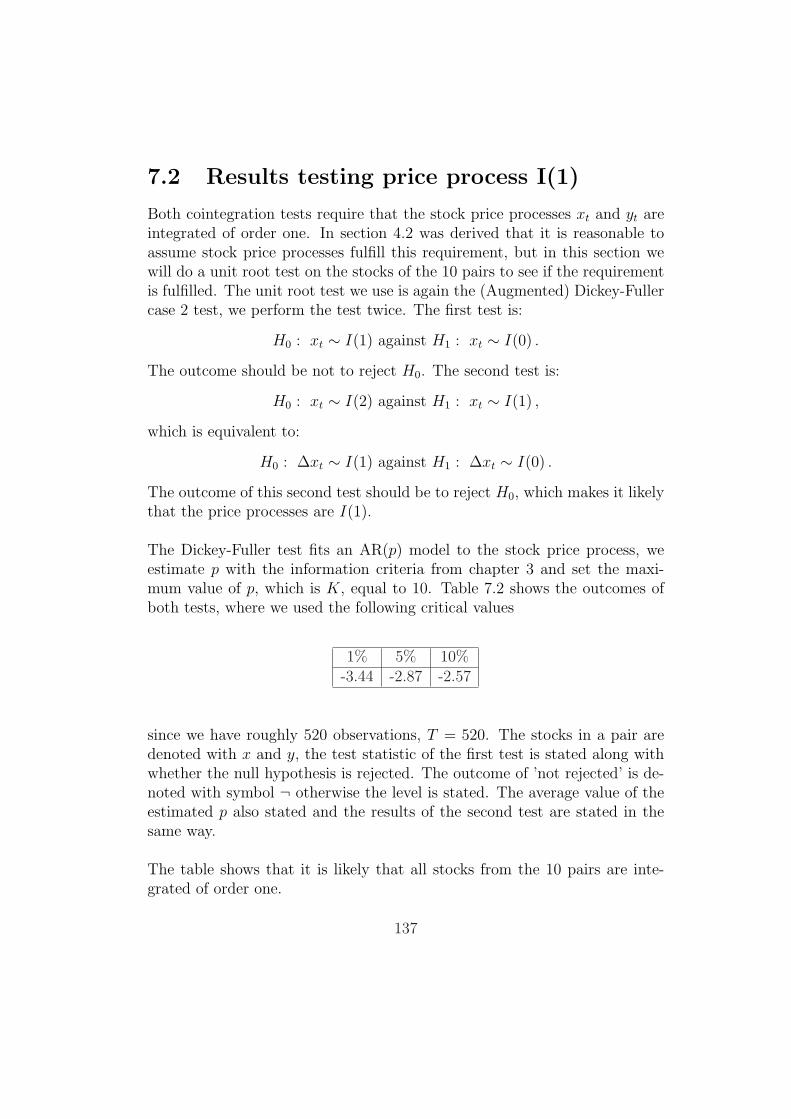
7.2 Results testing price process I(1)

Both cointegration tests require that the stock price processes xt and yt areintegrated of order one. In section 4.2 was derived that it is reasonable toassume stock price processes fulfill this requirement, but in this section wewill do a unit root test on the stocks of the 10 pairs to see if the requirementis fulfilled. The unit root test we use is again the (Augmented) Dickey-Fullercase 2 test, we perform the test twice. The first test is:

H0 : xt ∼ I(1) against H1 : xt ∼ I(0) .

The outcome should be not to reject H0. The second test is:

H0 : xt ∼ I(2) against H1 : xt ∼ I(1) ,

which is equivalent to:

H0 : ∆xt ∼ I(1) against H1 : ∆xt ∼ I(0) .

The outcome of this second test should be to reject H0, which makes it likelythat the price processes are I(1).

The Dickey-Fuller test fits an AR(p) model to the stock price process, weestimate p with the information criteria from chapter 3 and set the maxi-mum value of p, which is K, equal to 10. Table 7.2 shows the outcomes ofboth tests, where we used the following critical values

1% 5% 10%-3.44 -2.87 -2.57

since we have roughly 520 observations, T = 520. The stocks in a pair aredenoted with x and y, the test statistic of the first test is stated along withwhether the null hypothesis is rejected. The outcome of ’not rejected’ is de-noted with symbol ¬ otherwise the level is stated. The average value of theestimated p also stated and the results of the second test are stated in thesame way.

The table shows that it is likely that all stocks from the 10 pairs are inte-grated of order one.

137

Table 7.2: Results I(1).

Test 1 Test 2stock statistic outcome p statistic outcome pI -x -1.7 ¬ 4 -11 1% 4I -y -2.1 ¬ 4 -11 1% 4II -x -1.4 ¬ 1 -12 1% 3II -y -1.3 ¬ 2 -25 1% 1III -x -2.1 ¬ 1 -22 1% 1III -y -2.2 ¬ 1 -26 1% 1IV -x -1.4 ¬ 1 -24 1% 1IV -y -1.5 ¬ 1 -22 1% 1V -x -1.4 ¬ 8 -8 1% 8V -y -0.3 ¬ 10 -8 1% 10VI -x -0.6 ¬ 4 -12 1% 4VI -y -0.6 ¬ 4 -12 1% 4VII -x -1.1 ¬ 1 -25 1% 1VII -y -0.9 ¬ 1 -25 1% 1VIII -x -1.4 ¬ 1 -23 1% 1VIII -y -1.5 ¬ 1 -23 1% 1IX -x -1.4 ¬ 1 -25 1% 1IX -y -0.9 ¬ 1 -25 1% 1X -x -0.5 ¬ 2 -23 1% 1X -y -0.7 ¬ 1 -16 1% 2

7.3 Results Engle-Granger cointegration test

In this section we perform the Engle-Granger test on the 10 pairs. We havefound no reason to assume the Engle-Granger test statistic has a differentdistribution than the Dickey-Fuller case 2 test statistic, so we will use thesame critical values:

1% 5% 10%-3.44 -2.87 -2.57

138

We perform the cointegration test on the whole data set, so we have 520 ob-servations per stock. Recall that the profits were determined for the secondhalf of observations. As stated in section 4.3, the Engle-Granger method isnot symmetric. The results can be different for regressing xt on yt and theother way around. That is why we perform the Engle-Granger test twice.The results are stated in table 7.3.

Table 7.3: Results Engle-Granger test.

pair statistic 1 outcome α1 p statistic 2 outcome α2 pI -1.57 ¬ 1.53 6 -1.56 ¬ 0.65 6II -17.54 1% 0.997 1 -17.56 1% 1.003 1III -2.21 ¬ 0.72 3 -2.21 ¬ 1.37 3IV -2.67 10% 0.52 1 -2.61 10% 1.91 2V -1.04 ¬ 5.03 10 -1.08 ¬ 0.20 7VI -2.23 ¬ 1.08 3 -2.24 ¬ 0.93 3VII -4.65 1% 1.60 2 -4.64 1% 0.63 2VIII -2.92 5% 0.53 1 -2.91 5% 1.87 1IX -0.63 ¬ 2.36 2 -0.90 ¬ 0.42 1X -3.48 1% 0.72 1 -3.03 5% 1.39 4

We see that there is only one pair where the outcome of the two tests aredifferent, pair X. The estimated cointegrating relation are for all pairs prac-tically the same:

α1 ≈ 1/α2 .

So the disadvantage of the Engle-Granger method of not being symmetricdoes not seem to be very harmful when testing pairs for cointegration. Thepairs are put in order of the test statistic, the idea is that the lower teststatistic the lower the level of rejection, which is more evidence for beingcointegrated. For example, the Engle-Granger method rejects the null hy-pothesis for pair II even at 0.1% level, while pair VIII is only rejected at5%. So there is more evidence that pair II is cointegrated than pair VIII,which is why we prefer pair II.

139

The ordering of the 10 pairs based on the Engle-Granger method is

1 pair II2 pair VII3 pair X4 pair VIII5 pair IV6 pair VI7 pair III8 pair I9 pair V10 pair IX

where there is evidence for cointegration for the first five pairs, and no ev-idence for the remaining five. This ordering is not exactly the same as theordering found with the trading strategy, but they coincide on what is goodand what is not. The five pairs which are considered to be worthwhile trad-ing are cointegrated and the five pairs that are not worthwhile trading arenot cointegrated according to the Engle-Granger method. The first in bothorderings are the same, this is the pair that consists of two equal stocks butlisted on different exchanges. In the first half of the ordering, the good ones,only places 2 and 3 are switched, the others are at the same places. Thesecond half of the two orderings differ a lot.

7.4 Results Johansen cointegration test

In this section we perform the Johansen test on the 10 pairs. As discussedin section 4.4, we perform three tests:

Test 1 H0 : 0 relations against H1 : 2 relations.Test 2 H0 : 0 relations against H1 : 1 relation.Test 3 H0 : 1 relation against H1 : 2 relations.

The critical values for each test are in table 7.4, these are for a sample sizeof T = 400. Although the data of the 10 pairs IMC provided consist of 520observations, these critical values will be used when testing the 10 pairs forcointegration.

140

Table 7.4: Critical values for Johansen test.Test 1% 5% 10%

1 16.31 12.53 10.472 15.69 11.44 9.523 6.51 3.84 2.86

One issue that was not addressed in section 4.4 was how to find p. TheJohansen method assumes that the vector process yt = (xt, yt) follows aVAR(p) model. In S-PLUS, the program used for all simulations and calcu-lations in this report, exists a built-in function called ’ar’ which fits a VARmodel using Yule-Walker equations. The function determines the order ofthe VAR with the Akaike information criterion. This function is used forestimating p. We set the maximum value of p equal to 10 and the minimumvalue equal to 2 because the first step of the Johansen method is to fit aVAR(p − 1) on the differences ∆yt. The results of the Johansen test are intable 7.5.

Table 7.5: Results Johansen test.

Test 1 Test 2 Test 3 Parameterspair stat. 1 outcome stat. 2 outcome stat. 3 outcome p αI 6.80 ¬ 6.12 ¬ 0.68 ¬ 2 1.49II 154.6 1% 153.8 1% 0.82 ¬ 2 0.997III 7.37 ¬ 6.56 ¬ 0.81 ¬ 2 0.71IV 10.89 10% 10.43 10% 0.46 ¬ 2 0.52V 2.86 ¬ 2.79 ¬ 0.07 ¬ 4 5.44VI 6.47 ¬ 5.91 ¬ 0.56 ¬ 3 1.08VII 24.25 1% 23.10 1% 1.15 ¬ 2 1.59VIII 13.84 5% 13.16 5% 0.02 ¬ 2 0.52IX 2.78 ¬ 2.68 ¬ 0.11 ¬ 2 2.55X 14.98 5% 10.11 5% 1.98 ¬ 2 0.72

141

The Johansen method is symmetric, there is no difference if we set yt =(xt, yt) or yt = (yt, xt). The test statistics and the estimated cointegrationrelations are exactly the same. We consider the stocks of the pair being coin-tegrated if the null hypothesis of the first and the second test are rejectedand the null hypothesis of the third test is not rejected.

The Johansen method finds the same pairs cointegrated as the Engle-Grangermethod, pair II, IV, VII, VIII and X. The levels for rejection the null hypoth-esis of no cointegration are the same. Only for pair X the results differ a bit,but this is because the Engle-Granger method had two different outcomes,the first test had rejected at 1% and the second test at 5%. The Johansenmethod has rejected pair X at 5%. There are no real differences for thecointegrated pairs, the estimated cointegrating relations are also practicallythe same. The biggest difference is for pair VIII, where the Engle-Grangermethod estimates α equal to 5.338 and the Johansen method 5.231. Thetwo methods differ more for pairs that are not cointegrated, the differencesbetween the estimates of α are larger. But according to these methods thepairs are not cointegrated so there does not exist an α such that yt − αxt isstationary.

The ordering of the 10 pairs based on the Johansen method is

1 pair II2 pair VII3 pair VIII4 pair X5 pair IV6 pair III7 pair I8 pair VI9 pair V10 pair IX

where there is evidence for cointegration for the first five pairs, and no evi-dence for the remaining five. This ordering differs slightly from the Engle-Granger ordering. But most important is that the two methods coincide onwhich pairs are cointegrated and which are not. And this in turn coincideswith the results from the trading strategy.

142

Chapter 8

Conclusion

The goal of this project was to apply statistical techniques to find relation-ships between stocks. The closing prices of these stocks, dating back twoyears, are the only data that have been used in this analysis.

From trading experience, IMC is able to make a distinction between goodand bad pairs based on profits. In chapter 2 we derived a trading strategythat resembles the strategy used by IMC. From this strategy, we derived theimportant characteristics of a good pair. We saw that we like the price pro-cesses to be tied together such that their spread oscillates around zero anddoes not walk away.

In this report we tried to identify pairs with cointegration. If two stocksin a pair are cointegrated, a certain linear combination of the two is sta-tionary. This implies that this linear combination, which can be seen as thespread, is mean-reverting. This is in line with the characteristics of a goodpair.

In chapter 4 we introduced two methods for testing for cointegration, theEngle-Granger and the Johansen method. We have looked at the Engle-Granger method in detail. This method makes use of a unit root test, theDickey-Fuller test. Because there is a lot of ambiguity in the literature ofwhich Dickey-Fuller test and which critical values should be used, we dis-cussed the different cases in chapter 5. The asymptotic distributions of thetest statistics were derived and the critical values for finite sample sizes werefound with simulation.

143

In chapter 6 we examined the properties of the Engle-Granger method, whichconsists of a linear regression followed by the Dickey-Fuller test on the resid-uals of this regression. The main question was, which Dickey-Fuller caseto use and whether the critical values of the Engle-Granger method are thesame as those for this Dickey-Fuller test. We saw that case 2 was the mostappropriate one for the way we want to test for cointegration, that is with-out a constant in the cointegrating relation. There was no indication, basedon simulations, that the critical values from the Engle-Granger test differfrom those of the Dickey-Fuller case 2 test. Also the power of the two testswere found similar when the assumptions of the method were fulfilled. TheEngle-Granger test appeared to perform well, even when some assumptionswere not fulfilled. The Engle-Granger test assumes that the residuals followan autoregressive model. When we generated cointegrated data with residu-als that are not likely to be autoregressive, the method still rejects the nullhypothesis of no cointegration often.

IMC has provided a selection of ten pairs that are different in quality. Inchapter 7 we applied the trading strategy from chapter 2 to the historicalclosing prices. Based on profitability and the number of trades, we find adistinction between good and bad pairs which coincides with the distinctionmade by IMC. In this chapter we also tested the ten pairs for cointegration,using both the Engle-Granger as well as the Johansen method. The twomethods coincide on which pairs are cointegrated and which are not. Alsothe estimated cointegrating relations are almost the same. All the good pairsaccording to the trading strategy are seen as cointegrated, according to bothtests. Furthermore all bad pairs are seen as not cointegrated according toboth tests.

Based on the results of this project, we may conclude that cointegration isan appropriate concept to identify pairs suitable for IMC’s trading strategy.

144

Chapter 9

Alternatives &recommendations

In this chapter we briefly discuss some alternative trading strategies in thefirst section and give some recommendations for further research in the secondsection.

9.1 Alternative trading strategies

In this report we focused on pair trading with two stocks in a pair. Twostocks being cointegrated is easily translated in the trading strategy fromchapter 2, we take the spread process as the linear combination of the twostocks corresponding to the cointegrating vector:

yt − αxt.

If we would take r from chapter 2 as the least squares estimate instead ofthe average ratio, the spread process of chapter 2 would be exactly the sameas the spread process found with the Engle-Granger method. That is if weuse the strategy without adjustment parameter κ, i.e., κ = 0.

In section 4.3 was stated that we neglect a possible constant in the coin-tegrating relation, α0. In this section we will look at a trading strategy thatdoes not neglect the constant. We also look at what can happen if we havecointegration between the logarithms of the stock prices.

145

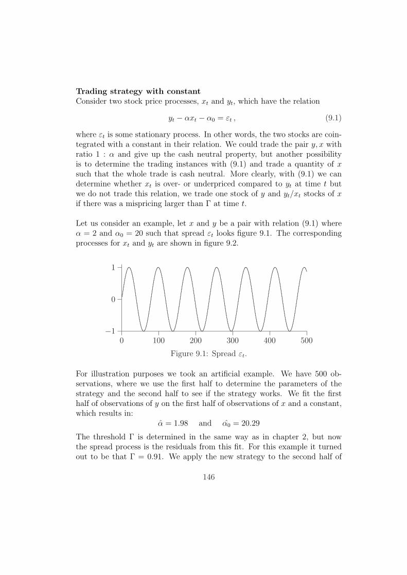
Trading strategy with constantConsider two stock price processes, xt and yt, which have the relation

yt − αxt − α0 = εt , (9.1)

where εt is some stationary process. In other words, the two stocks are coin-tegrated with a constant in their relation. We could trade the pair y, x withratio 1 : α and give up the cash neutral property, but another possibilityis to determine the trading instances with (9.1) and trade a quantity of xsuch that the whole trade is cash neutral. More clearly, with (9.1) we candetermine whether xt is over- or underpriced compared to yt at time t butwe do not trade this relation, we trade one stock of y and yt/xt stocks of xif there was a mispricing larger than Γ at time t.

Let us consider an example, let x and y be a pair with relation (9.1) whereα = 2 and α0 = 20 such that spread εt looks figure 9.1. The correspondingprocesses for xt and yt are shown in figure 9.2.

0 100 200 300 400 500−1

0

1

........

.........

.........

.....................................................................................................................................................................................................................................................................................................................................................................................

..................................................................................................................................................................................................................................................................................................................................................................................................................................................................................................................................................

..................................................................................................................................................................................................................................................................................................................................................................................................................................................................................................................................................

..................................................................................................................................................................................................................................................................................................................................................................................................................................................................................................................................................

...................................................................................................................................................................................................................................................................................................................................................................................................................................................................................................................................................

..................................................................................................................................................................................................................................................................................................................................................................................................................................................................................................................................................

...................................................................................................................................................................................................................................................................................

Figure 9.1: Spread εt.

For illustration purposes we took an artificial example. We have 500 ob-servations, where we use the first half to determine the parameters of thestrategy and the second half to see if the strategy works. We fit the firsthalf of observations of y on the first half of observations of x and a constant,which results in:

α = 1.98 and α0 = 20.29

The threshold Γ is determined in the same way as in chapter 2, but nowthe spread process is the residuals from this fit. For this example it turnedout to be that Γ = 0.91. We apply the new strategy to the second half of

146

0 100 200 300 400 500

20

40

60

80

..................................................................................................................................................................................................................................................................................................................................................................................

........................................................................................................................................................................................................................................................................................................................................................................................................................

...........................................................................................................................................................................................

...........................................................................

......................................................................................................................................................................................................................................................................................................................................

.............................................................................................

................................................................................................................................................

............................................................................................................

................................................................................................................

.............................................................................................................................................

........................................................................................................................

......................................................................................................................................................................................................................

Figure 9.2: Price processes xt and yt.

observations. The trades are shown in table 9.1. With the first trade we puton a position for the first time, so we made no profit yet. The second tradeconsists of two parts, we flatten the position from the first trade which resultsin a profit and we put on a new position. We always trade one stock of y andwe trade yt/xt number of stocks x so it is exactly cash neutral. The actualtraded spread is not shown because it is basically the same as the right halfof figure 9.1. Figure 9.3 shows the spread if we do not include a constant,i.e., if we neglected α0.

Table 9.1: Trading instances.trade t st position (y,x) price yt price xt profit

1 251 0.91 (-1,+2.82) 72.08 25.59 -2 291 -0.93 (+1,-2.80) 66.87 23.90 0.443 331 0.93 (-1,+2.85) 70.20 24.63 1.274 370 -0.91 (+1,-2.73) 71.03 25.98 2.995 409 0.95 (-1,+2.74) 77.65 28.37 0.076 452 -0.94 (+1,-2.66) 77.05 29.02 2.377 487 0.93 (-1,+2.71) 79.86 29.49 1.55

total profit 8.69

Although the profit for each trade is not at least 2Γ, as the profit for thetrading strategy from chapter 2 with constant ratio was, it is still quite prof-itable to trade this pair this way. Specially because the trading strategy fromchapter 2 would not make any money, even if we would have used a largeadjustment parameter κ.

147

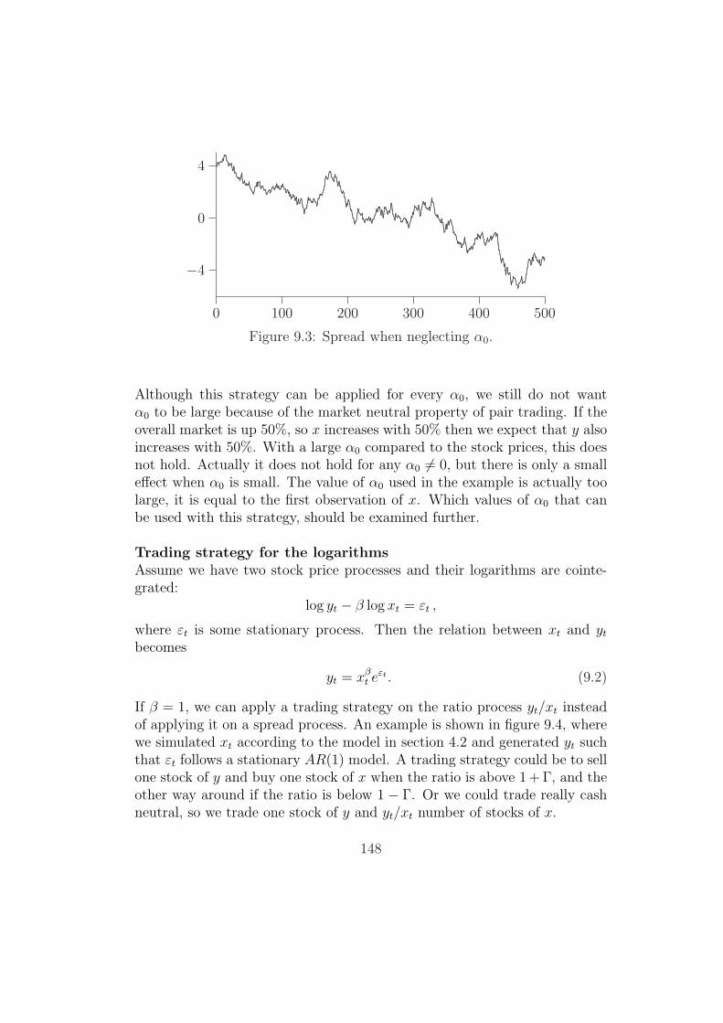
0 100 200 300 400 500

−4

0

4 ...........................................................................................................................

..................................................................................................................................................................

.......................................................................................................

.................................................................................................

...............................................................................................................................................................................................................................................................................

........................................................................................................................................................................................................................................................................................................

..........................................................................................................................................................................

........................................................................................................................................................................................................

.........

........................................................................................................

....................................................................................................................................................................................................................................................

.....................................................................................................

..............................................................................................................................................................................................................

........................................................................................................................................................................................................................................................................................................................................................................

.............................................................................................................................

........

...............................................................................................................................................................................................................................................................

.............................

Figure 9.3: Spread when neglecting α0.

Although this strategy can be applied for every α0, we still do not wantα0 to be large because of the market neutral property of pair trading. If theoverall market is up 50%, so x increases with 50% then we expect that y alsoincreases with 50%. With a large α0 compared to the stock prices, this doesnot hold. Actually it does not hold for any α0 6= 0, but there is only a smalleffect when α0 is small. The value of α0 used in the example is actually toolarge, it is equal to the first observation of x. Which values of α0 that canbe used with this strategy, should be examined further.

Trading strategy for the logarithmsAssume we have two stock price processes and their logarithms are cointe-grated:

log yt − β log xt = εt ,

where εt is some stationary process. Then the relation between xt and yt

becomes

yt = xβt eεt . (9.2)

If β = 1, we can apply a trading strategy on the ratio process yt/xt insteadof applying it on a spread process. An example is shown in figure 9.4, wherewe simulated xt according to the model in section 4.2 and generated yt suchthat εt follows a stationary AR(1) model. A trading strategy could be to sellone stock of y and buy one stock of x when the ratio is above 1 + Γ, and theother way around if the ratio is below 1 − Γ. Or we could trade really cashneutral, so we trade one stock of y and yt/xt number of stocks of x.

148

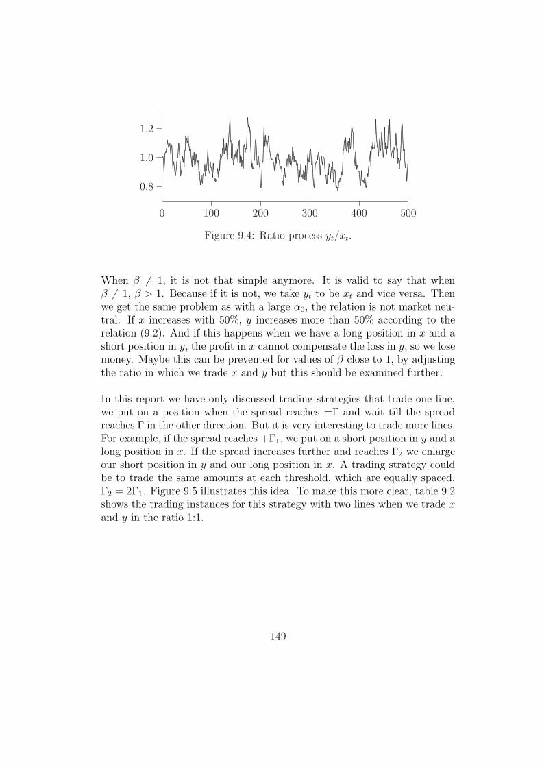
0 100 200 300 400 500

0.8

1.0

1.2

...................................................................................................................................................................................................................................................................................................................................................................................................................................................................................................................................................................................................................................................................................................................................................................................................................................................................................................................................................................................................................................................................................................................................................................................................................................................................................................................................................................................................................................................................................................................................................................................................................................................................................................................................................................................................................................................................................................................................................................................................................................................................................................................................................................................................................................................................................................................................................................................................................................................................................................................................................................................................................................................................................................................................................................................................................................................................................................................................................................................................................................................................................................................................................................................................................................................................................................................................................................................................................................................................................................................................................................................................................................................................................................................................................................................................................................................................................................................................................................................................................................................................................................................................

................................................................................................................................................................................................................................

........

........

..................................................................................................................................................................................................................................................................................................................................................................................................................................................................................................

........

........

........

...........................................................................................................................................................................................................................................................................................................................................................................................................................................................................................................................................................................................................................................................................................................................................................................................................................................................................................................................................................................................................................................................................................................................................................................................................................................................................................................................................................................................................................................................................................................................................................................................................................................................................................................................................................................................................................................................................................................................................................................................................................................................................................................................................................................................................................................................................................................................................................................................................................................................................................................................................................................................................................................................................................................................................................................................................................................................................................................................................................................................................................................................................................................................................................................................................................................................................................................................................................................................................................................................................................................................................................................................................................................................................................................................................................................................................................................................................................................................................................................................................................................................................................

Figure 9.4: Ratio process yt/xt.

When β 6= 1, it is not that simple anymore. It is valid to say that whenβ 6= 1, β > 1. Because if it is not, we take yt to be xt and vice versa. Thenwe get the same problem as with a large α0, the relation is not market neu-tral. If x increases with 50%, y increases more than 50% according to therelation (9.2). And if this happens when we have a long position in x and ashort position in y, the profit in x cannot compensate the loss in y, so we losemoney. Maybe this can be prevented for values of β close to 1, by adjustingthe ratio in which we trade x and y but this should be examined further.

In this report we have only discussed trading strategies that trade one line,we put on a position when the spread reaches ±Γ and wait till the spreadreaches Γ in the other direction. But it is very interesting to trade more lines.For example, if the spread reaches +Γ1, we put on a short position in y and along position in x. If the spread increases further and reaches Γ2 we enlargeour short position in y and our long position in x. A trading strategy couldbe to trade the same amounts at each threshold, which are equally spaced,Γ2 = 2Γ1. Figure 9.5 illustrates this idea. To make this more clear, table 9.2shows the trading instances for this strategy with two lines when we trade xand y in the ratio 1:1.

149

0 100 200 300

−4

−2

0

2

4

.................................................................................................................................................................................................................................................................

........

........

........

........

..................................................................................................................................................................................................................................................................................................................................................................................................................................................................................................................................................................................................................

.........

........

........

..............................................................................................................................................................................................................................................................................................................................................................................................................................................................................................................................................................................................................................................

........

........

.........

........

..................................................................................................................................................

........................................................................................................................................................................................................................................................................................................................

...............................................................................................................................................................................................................................................................................................................................................................

........

...............................................................................................................................................................................................................................................................................................................................................................................................................................................................................................................................................................................................................

........

.................................................................................................................................................................................................................................................................................................................................................................................................................................................................................................................................................................................................................................................................................

........................................................................................................................................................................................................................................................................................................................................................................................

........

........

.........

........

........

........

.........

........

........

.................................................................................................................................................................................................................................................................................................................................................................................................................

........

........

.........................................................................................................................

................................................................................................................................................................................................................................................................................................................................................................................................................................................................................................................................................................................................................................................................................................

............. ............. ............. ............. ............. ............. ............. ............. ............. ............. ............. ............. ............. ............. ............. ............. ............. ............. ............. ............. ............. ............. ............. ............. ............. ............. .............

............. ............. ............. ............. ............. ............. ............. ............. ............. ............. ............. ............. ............. ............. ............. ............. ............. ............. ............. ............. ............. ............. ............. ............. ............. ............. .............

. . . . . . . . . . . . . . . . . . . . . . . . . . . . . . . . . . . . . . . . . . . . . . . . . . . . . .

. . . . . . . . . . . . . . . . . . . . . . . . . . . . . . . . . . . . . . . . . . . . . . . . . . . . . .

Figure 9.5: A 2 line strategy.

This strategy can be easily extended to more lines, it can even be easilyextended to three or more stocks in a pair. How to choose the number oflines, the thresholds and the corresponding amount of stocks is very inter-esting to examine further.

9.2 Recommendations for further research

It would be nice to develop the alternative method from section 4.5 further,such that we have a new method for testing for cointegration. In order todo so, we need an accurate algorithm for the estimation of the parameters ofthe MA(q) model.

In this report we used closing prices. It is interesting to apply the tradingstrategies and cointegration tests to intra-day data because we trade duringthe day. This is specially interesting if we have a trading strategy with alarge number of lines with the thresholds close to each other.

We could cut the cointegration test into several pieces. Suppose we havedatasets containing four years of closing prices, than we could perform threetests on two years of data with an overlap of one year. More clearly, thefirst test is on the first and second year, the second test is on the second and

150

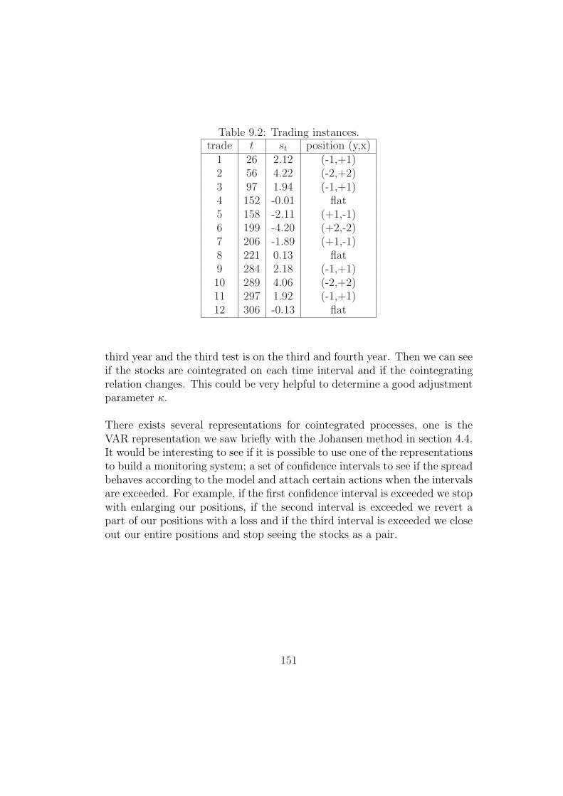
Table 9.2: Trading instances.trade t st position (y,x)

1 26 2.12 (-1,+1)2 56 4.22 (-2,+2)3 97 1.94 (-1,+1)4 152 -0.01 flat5 158 -2.11 (+1,-1)6 199 -4.20 (+2,-2)7 206 -1.89 (+1,-1)8 221 0.13 flat9 284 2.18 (-1,+1)10 289 4.06 (-2,+2)11 297 1.92 (-1,+1)12 306 -0.13 flat

third year and the third test is on the third and fourth year. Then we can seeif the stocks are cointegrated on each time interval and if the cointegratingrelation changes. This could be very helpful to determine a good adjustmentparameter κ.

There exists several representations for cointegrated processes, one is theVAR representation we saw briefly with the Johansen method in section 4.4.It would be interesting to see if it is possible to use one of the representationsto build a monitoring system; a set of confidence intervals to see if the spreadbehaves according to the model and attach certain actions when the intervalsare exceeded. For example, if the first confidence interval is exceeded we stopwith enlarging our positions, if the second interval is exceeded we revert apart of our positions with a loss and if the third interval is exceeded we closeout our entire positions and stop seeing the stocks as a pair.

151

152

Bibliography

[1] C. ALEXANDER. Market Models. John Wiley & Sons, 2001.

[2] P.J. BROCKWELL and R.A. DAVIS. Introduction to time series andforecasting. Springer-Verlag, 2002.

[3] P.J. BROCKWELL and R.A. DAVIS. Time Series: Theory and Meth-ods. 1987, Springer-Verlag.

[4] D.A. DICKEY and W.A. FULLER. Distribution of the estimators forautoregressive time series with a unit root. Journal of the AmericanStatistical Association, 74:427–431, 1979.

[5] R.F. ENGLE and C.W.J. GRANGER. Co-integration and error correc-tion: Representation, estimation, and testing. Econometrica, 55(2):251–276, 1987.

[6] J.D. HAMILTON. Time Series Analysis. Princeton University Press,1994.

[7] D.J. HIGHAM. An introduction to financial option valuation. Cam-bridge University Press, 2004.

[8] S. JOHANSEN. Statistical analysis of cointegration vectors. Journal ofEconomic Dynamics and Control, 12:231–254, 1988.

[9] S. JOHANSEN. Estimation and hypothesis testing of cointegration vec-tors in guassian vector autoregressive models. Econometrica, 59:1551–1580, 1991.

[10] S. JOHANSEN and K. JUSELIUS. Maximum likelihood estimation andinference of cointegration - with application to the demand for money.Oxford Bulletin of Economics and Statistics, 52:208, 1990.

153

[11] M. OSTERWALD-LENUM. A note with quantiles of the asymptoticdistribution of the maximum likelihood cointegration rank test statistics.Oxford Bulletin of Economics and Statistics, 54:462, 1992.

[12] P.C.B. PHILIPS and S.N. DURLAUF. Multiple time series regressionwith integrated processes. Review of Economic Studies, 53:473–495,1986.

[13] P.C.B. PHILIPS and S. OULIARIS. Asymptotic properties of residualbased tests for cointegration. Econometrica, 58(1):165–193, 1990.

[14] J.H. STOCK and M.W. WATSON. Testing for common trends. Journalof the American Statistical Association, 83(404):1097–1107, 1988.

[15] G. VIDYAMURTHY. Pairs Trading. John Wiley & Sons, 2004.

154