Getting started with R and R commanderGetting started with R and R commander Robin Beaumont...

$Page 1: Getting started with R and R commanderGetting started with R and R commander Robin Beaumont robin@organplayers.co.uk C:\web_sites_mine\HIcourseweb new\stats\basics\Rcmdr_and_R.docx$
Getting started with R

and R commander

Written by: Robin Beaumont e-mail: [email protected]

Date last updated Friday, 29 October 2010

Version: 1

A statistical analysis, properly conducted, is a

delicate dissection of uncertainties,

a surgery of suppositions.

M.J.Moroney

Getting started with R and R commander

Robin Beaumont [email protected] C:\web_sites_mine\HIcourseweb new\stats\basics\Rcmdr_and_R.docx page 2 of 19

Contents

1. INSTALLING R................................................................................................................................................................... 3

2. THE BASICS ...................................................................................................................................................................... 4

2.1 THE ASSIGNMENT/ GETS OPERATOR <- ............................................................................................................................. 4 2.2 # THE COMMENT (#) AND LINE EXTENSION ( + ) SYMBOLS IN R ........................................................................................... 4 2.3 FUNCTIONS ................................................................................................................................................................. 4

3. ENTERING DATA INTO R .................................................................................................................................................. 5

3.1 USING THE CONCATENATE FUNCTION C ............................................................................................................................ 5 3.2 CREATING LISTS AND DATAFRAMES .................................................................................................................................. 6

3.2.1 Factors – grouping variables............................................................................................................................... 6 3.2.2 Tables.................................................................................................................................................................. 7

3.3 READING DATA FROM A FILE ........................................................................................................................................... 7 3.3.1 Excel export – tab delimited .txt files .................................................................................................................. 7 3.3.2 text files .............................................................................................................................................................. 8 3.3.3 SPSS .sav files ...................................................................................................................................................... 8 3.3.4 Overview ............................................................................................................................................................. 8

4. EDITING THE DATASET .................................................................................................................................................... 9

5. SAVING DATA ................................................................................................................................................................ 11

6. MANIPULATING COLUMNS/ ROWS OF DATA .............................................................................................................. 11

7. GRAPHICAL INTERFACES TO R....................................................................................................................................... 13

7.1 R COMMANDER (THE RCMDR PACKAGE) ......................................................................................................................... 13 7.1.1 Reading in data ................................................................................................................................................. 13 7.1.2 Creating / Editing datasets ............................................................................................................................... 14 7.1.3 Manipulating data ............................................................................................................................................ 14 7.1.4 Saving Data ....................................................................................................................................................... 15 7.1.5 Descriptive statistics ......................................................................................................................................... 15 7.1.6 Inferential statistics and models ....................................................................................................................... 16 7.1.7 Intelligent menus .............................................................................................................................................. 17

7.2 DEDUCER ................................................................................................................................................................. 17

8. SUMMARY ..................................................................................................................................................................... 18

9. APPENDIX - UPDATING R FOR WINDOWS .................................................................................................................... 19

9.1 SEEING THE PACKAGES YOU HAVE INSTALLED AND THEIR MANUAL INSTALLATION. .................................................................... 19 9.2 SEEING WHERE YOUR PACKAGES ARE INSTALLED AND COPYING THEM ALL AT ONCE .................................................................. 19



1. Installing R

Download the appropriate copy of R from http://www.r-project.org/

If you have a windows system you need to choose the binary version, there are versions for both 32 and 64 byte operating systems. Versions are also available for Mac and Linux operating systems.

Having installed R you can add a lot of free extensions (called packages) to the core program, this is discussed later.

One of the most basic things you can do with R is to treat it as a posh calculator.

Exercise

Install R and type in the R console window the expression opposite and also on the following line the name you gave the expression to bring up the result.

http://www.r-project.org/



2. The basics

R has what is known as a command line interface, that is you type in one or more commands into a window which is called the R console, this is in complete contrast to the point and click approach that you are used to using in windows.

The commands you type in follow certain grammatical rules (called syntax) and below are some important details to help you understand them.

2.1 The assignment/ gets operator <-

In R a variable is assigned (i.e. given) a value using the assignment/gets operator which looks like: <-, that is a less than symbol followed by the minus sign, think of it as equivalent to the equals sign. For example say we want to assign the value of 10 to the variable 'myresult' we would do this by typing into R:

myresult <- 10

Similarly we can make myresult equal a complex expression such as myresult <- 2*sqrt(4*pi), here it equals an expression that uses multiplication (*), square root (sqrt) and π (pi). A variable may also consist of more than one value, each called an element as we will see in the following sections.

2.2 # The comment (#) and line extension ( + ) symbols in R

The # hash character is used to indicate that the rest of the line is to be treated as a comment, for example:

length(x) # this is all a comment and ignored by R but helps me understand it

Similarly if you want to create a single command over several lines you just add the space and plus character + at the end and beginning of the next line in R

2.3 Functions

R has a large number of very useful functions which you can apply to your variables. The reference list below gives you a flavour, at this stage you are not expected to understand most of them.

* multiplication

^ exponent i.e. 2^ 3 means 2 cubed

Sqrt(x) square root

max(x), min(x), mean(x), median(x), sum(x), var(x), sd(x), cor(x,y) as named for variable x

summary(data.frame) prints statistics

rank(x), sort(x) rank and sort variable x

ave(x,y) averages of x grouped by factor y

sin, cos, tan, asin, acos, atan, atan2, log, log10, exp as named

range(x) range

round(x, n) rounds the elements of x to n decimals

log(x, base) computes the logarithm of x with base base

mod(x) modulus; abs(x) is the same

Notice that R is case sensitive Mod does not mean the same a MOD or mOD!!

Taken from http://cran.r-project.org/doc/contrib/refcard.pdf R reference card, by Jonathan Baron and http://cran.r-project.org/doc/contrib/Short-refcard.pdf R reference card, by Tom Short

http://cran.r-project.org/doc/contrib/refcard.pdf

http://cran.r-project.org/doc/contrib/Short-refcard.pdf

http://cran.r-project.org/doc/contrib/Short-refcard.pdf



3. Entering data into R

There are many ways to do this I will present three here.

Using the concatenate function

Creating dataframes

Reading in data from files and attaching to a dataframe

3.1 Using the concatenate function c

Say we want to enter a set of values for a particular variable, you can think of these values as representing a column (vector in technical language), and we use the 'c' = concatenate function to do this.

Exercise

Do what is shown in the window opposite. Also type in:

plot(x,y) # what do you get?

mean(x) # what do you get?

var(x) # what do you get?

sd(x) # what do you get?

length(x) # what do you get?

Notice that R is case sensitive plot does not mean the same a PLOT or Plot!!

Also try the summary command

To be able to analyse data in various groups we need to structure it and this is described in the next section.



3.2 Creating lists and dataframes

R prefers it if you create some type of structure for your data in what it calls either a list or a dataframe.

A list can have variables with unequal numbers of items but in a dataframe all the columns (vectors) must be the same length.

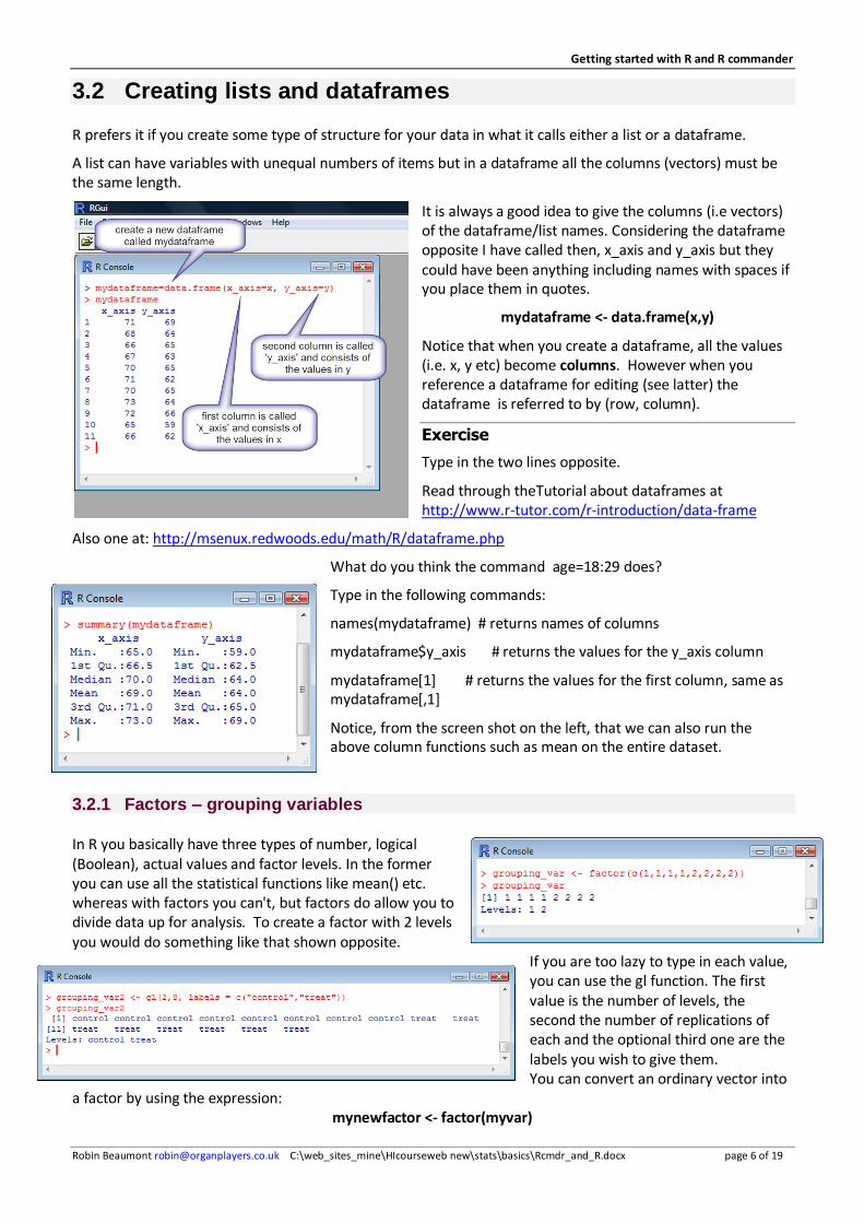
It is always a good idea to give the columns (i.e vectors) of the dataframe/list names. Considering the dataframe opposite I have called then, x_axis and y_axis but they could have been anything including names with spaces if you place them in quotes.

mydataframe <- data.frame(x,y)

Notice that when you create a dataframe, all the values (i.e. x, y etc) become columns. However when you reference a dataframe for editing (see latter) the dataframe is referred to by (row, column).

Exercise

Type in the two lines opposite.

Read through theTutorial about dataframes at http://www.r-tutor.com/r-introduction/data-frame

Also one at: http://msenux.redwoods.edu/math/R/dataframe.php

What do you think the command age=18:29 does?

Type in the following commands:

names(mydataframe) # returns names of columns

mydataframe$y_axis # returns the values for the y_axis column

mydataframe[1] # returns the values for the first column, same as mydataframe[,1]

Notice, from the screen shot on the left, that we can also run the above column functions such as mean on the entire dataset.

3.2.1 Factors – grouping variables

In R you basically have three types of number, logical (Boolean), actual values and factor levels. In the former you can use all the statistical functions like mean() etc. whereas with factors you can't, but factors do allow you to divide data up for analysis. To create a factor with 2 levels you would do something like that shown opposite.

If you are too lazy to type in each value, you can use the gl function. The first value is the number of levels, the second the number of replications of each and the optional third one are the labels you wish to give them. You can convert an ordinary vector into

a factor by using the expression: mynewfactor <- factor(myvar)

http://www.r-tutor.com/r-introduction/data-frame

http://msenux.redwoods.edu/math/R/dataframe.php



3.2.2 Tables

The first thing most people do with a set of data is divide it up often producing tables and graphs. In R both these things are easily achievable.

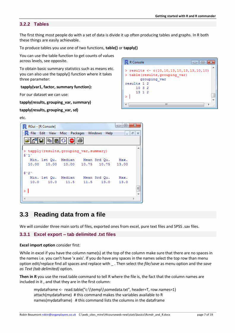
To produce tables you use one of two functions, table() or tapply()

You can use the table function to get counts of values across levels, see opposite.

To obtain basic summary statistics such as means etc. you can also use the tapply() function where it takes three parameter:

tapply(var1, factor, summary function):

For our dataset we can use:

tapply(results, grouping_var, summary)

tapply(results, grouping_var, sd)

etc.

3.3 Reading data from a file

We will consider three main sorts of files, exported ones from excel, pure text files and SPSS .sav files.

3.3.1 Excel export – tab delimited .txt files

Excel import option consider first:

While in excel if you have the column name(s) at the top of the column make sure that there are no spaces in the names i.e. you can't have 'x axis'. If you do have any spaces in the names select the top row than menu option edit/replace find all spaces and replace with _ . Then select the file/save as menu option and the save as Text (tab delimited) option.

Then in R you use the read.table command to tell R where the file is, the fact that the column names are included in it , and that they are in the first column:

mydataframe <- read.table("c:\\temp\\somedata.txt", header=T, row.names=1) attach(mydataframe) # this command makes the variables available to R names(mydataframe) # this command lists the columns in the dataframe



3.3.2 text files

In R use the command:

mydataframe <- read.table(file=file.choose()) # allow you to select the file from the popup dialog box.

attach(mydataframe) # this command makes the variables available to R

For more details see: http://msenux.redwoods.edu/math/R/ImportingData.php

3.3.3 SPSS .sav files

For R to be able to read SPSS .sav files, you can use the Rcmdr package (described latter) or you need to load the foreign package which is automatically installed when you install R. You can then use the read.spss command and the file.choose command to get the file name, alternatively you can type it in directly. In the code below I then assign the data to a mydata dataframe.

require(foreign) mydata <- read.spss(file=file.choose()) # allows you to select a file and places it in # the mydata dataframe, now see what I have imported: names(mydata) # lists the field names

Exercise

If you have excel, create a few columns of data, with the column names at the top of each column and then follow the above instructions – export the data and import into R.

If the have any .sav SPSS files follow the instructions above and see if you can successfully import one into R.

For other nice tutorials on R see: http://msenux.redwoods.edu/math/R/

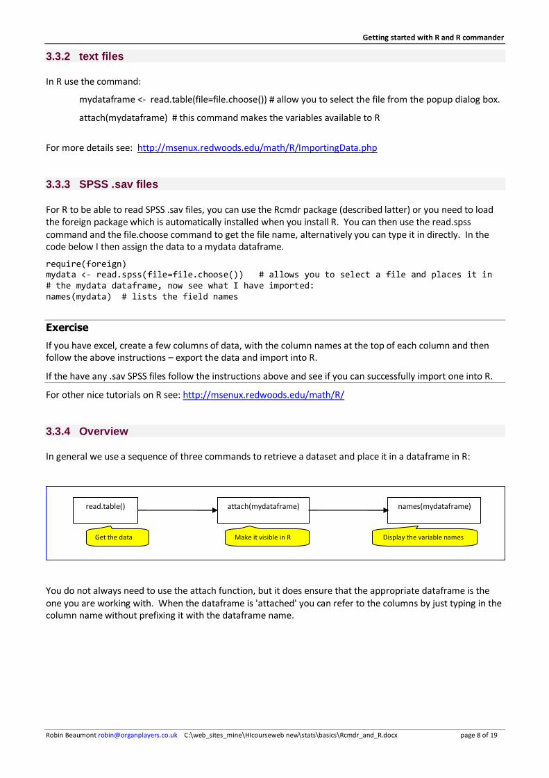
3.3.4 Overview

In general we use a sequence of three commands to retrieve a dataset and place it in a dataframe in R:

You do not always need to use the attach function, but it does ensure that the appropriate dataframe is the one you are working with. When the dataframe is 'attached' you can refer to the columns by just typing in the column name without prefixing it with the dataframe name.

read.table() attach(mydataframe) names(mydataframe)

Get the data Make it visible in R Display the variable names

http://msenux.redwoods.edu/math/R/ImportingData.php

http://msenux.redwoods.edu/math/R/



4. Editing the dataset

The easiest way to edit individual data items is to use the edit window, you can call up the window assuming that you have a dataframe called mydata by simply typing data.entry(mydata) or fix(mydata) when you close the window by clicking on the top right hand corner X any changes you have make are saved to the mydata dataframe. Obviously to save the changes to your permanent storage you need to save the dataset (see the next section). You can also use mydata <- edit(mydata), and can save the changes to another copy myNewdata <- edit(myolddata), then use attach(myNewdata) to use it.

You can also edit, individual items, columns (vectors) or rows by using various R commands. These are listed below. The important thing to remember is that we reference the dataframe considering the row and then the column.

Mydataset(row , column)

Action R

Edit a row Change all the values in row 2 to equal 44

mydataframe[2,] <- 44

Edit a column Change all the values in column 1 to equal

100

mydataframe[,1] <- 100

or

mydataframe$"x column" <- 100

Edit a value Change the value in row 1, column 1 to

equal 3

mydataframe[1,1] <- 3

or

mydataframe$"x column"[1] <- 100

Action R

Renaming a column

Rename the first column to x_renamed

names (mydataframe) [1] <- c("x-renamed")

Adding a column(s)

Add three new columns, each with a different

value

mydataframe["newvar1"] <- 1 mydataframe["newvar2"] <- 0

mydataframe["newvar3"] <- 50

Deleting a column

Delete the column called newvar2

mydataframe["newvar2"] <- NULL



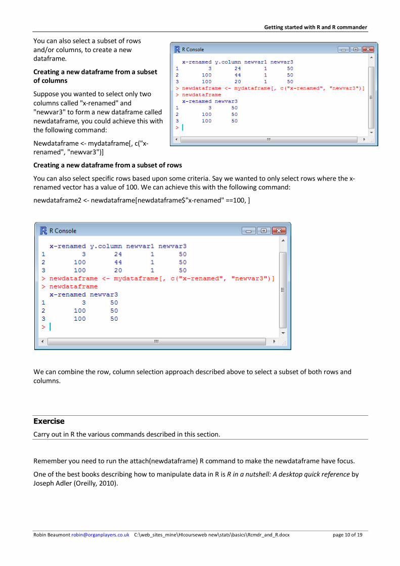
You can also select a subset of rows and/or columns, to create a new dataframe.

Creating a new dataframe from a subset of columns

Suppose you wanted to select only two columns called "x-renamed" and "newvar3" to form a new dataframe called newdataframe, you could achieve this with the following command:

Newdataframe <- mydataframe[, c("x-renamed", "newvar3")]

Creating a new dataframe from a subset of rows

You can also select specific rows based upon some criteria. Say we wanted to only select rows where the x-renamed vector has a value of 100. We can achieve this with the following command:

newdataframe2 <- newdataframe[newdataframe$"x-renamed" ==100, ]

We can combine the row, column selection approach described above to select a subset of both rows and columns.

Exercise

Carry out in R the various commands described in this section.

Remember you need to run the attach(newdataframe) R command to make the newdataframe have focus.

One of the best books describing how to manipulate data in R is R in a nutshell: A desktop quick reference by Joseph Adler (Oreilly, 2010).



5. Saving data

In R there are many ways to do this. You can also save, not just the data but the commands and output from a R session. For this basic introduction I will only explain how to save data.

To save the active dataset use the command:

save("mydataframe", file="C:/temp/mydataframe.rda") # note the rda =dataset extension

Or

require(tcltk) # use the dialog boxes that are available fileName <- tclvalue(tkgetSaveFile()) # ask user name and place to save file write.table(mydata, fileName, sep = "\t") # or type in filename directly i.e. "c:/mydata.txt"

# and to read this file back into R one needs myfile<- file.choose() # ask the user where the file is # now read the file into mydata dataframe mydata <- read.table(myfile, header = TRUE, sep = "\t", row.names = 1) To save a SPSS . sav file you use different commands:

require(foreign) # use the foreign package require(tcltk) # use the dialog boxes that are available datafileName <- tclvalue(tkgetSaveFile()) # ask user name and place to save sav file confileName <- tclvalue(tkgetSaveFile()) # ask user name and place to command file write.foreign(mydata, datafileName, confileName, package="SPSS") # or type in filenames directly in the above

Probably the easiest way to import and export SPSS files is to use the R commander interface – see below for details. SPSS itself has an extension which allows you to use R from within SPSS it is called the SPSS-R Integration Plugin (freeware) which, after registering, you can download from SPSS's website.

6. Manipulating columns/ rows of data

This section is for reference.

Often we have data in several columns (vectors) we wish to combine into a single one (vector), or alternatively we have data in one long column (vector) we wish to split into several columns (vectors).

Lets demonstrate this with two lists which we convert into one using the stack function, details shown opposite.

If we were considering a dataframe the stack function might be a bit more complex

stack(x, select, ...)

where select indicates which vectors to use.

But you can still easily put all the vectors in a single one very easily (see opposite).



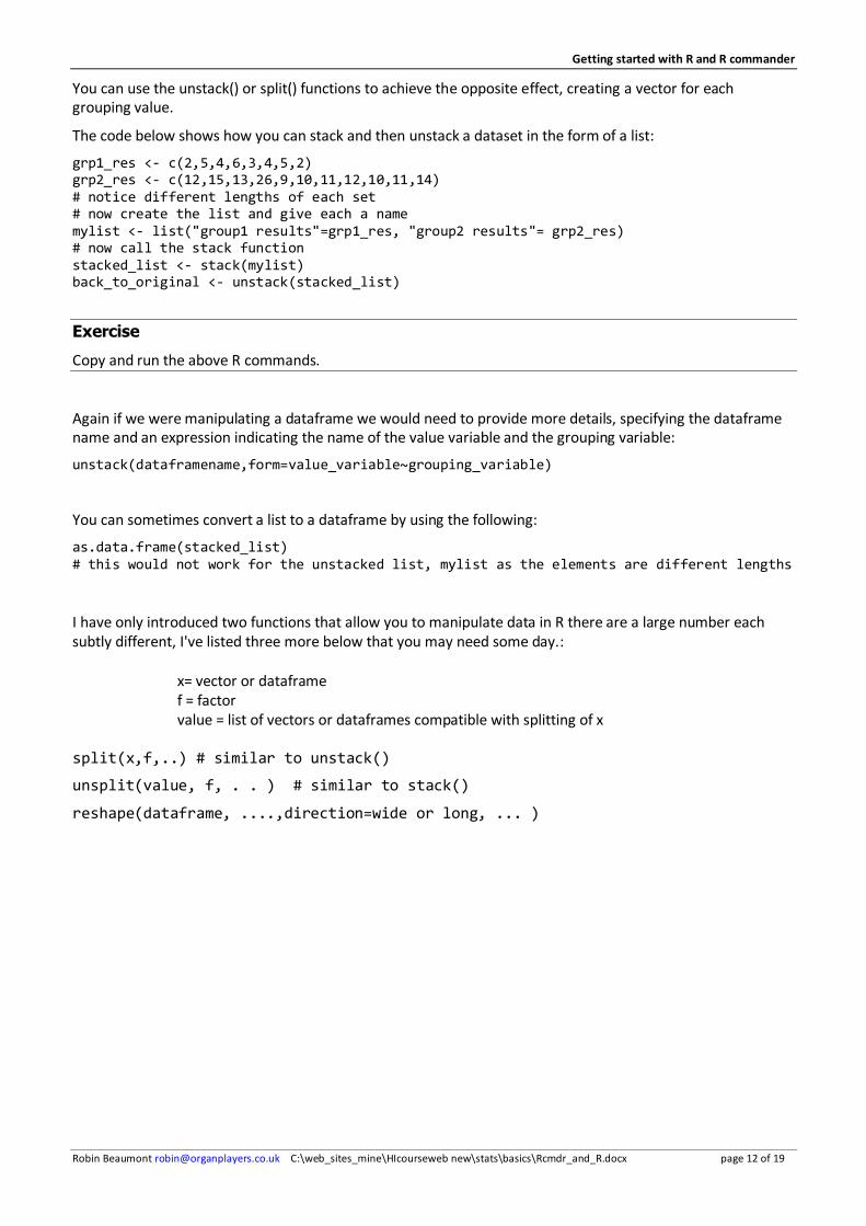
You can use the unstack() or split() functions to achieve the opposite effect, creating a vector for each grouping value.

The code below shows how you can stack and then unstack a dataset in the form of a list:

grp1_res <- c(2,5,4,6,3,4,5,2) grp2_res <- c(12,15,13,26,9,10,11,12,10,11,14) # notice different lengths of each set # now create the list and give each a name mylist <- list("group1 results"=grp1_res, "group2 results"= grp2_res) # now call the stack function stacked_list <- stack(mylist) back_to_original <- unstack(stacked_list)

Exercise

Copy and run the above R commands.

Again if we were manipulating a dataframe we would need to provide more details, specifying the dataframe name and an expression indicating the name of the value variable and the grouping variable:

unstack(dataframename,form=value_variable~grouping_variable)

You can sometimes convert a list to a dataframe by using the following:

as.data.frame(stacked_list) # this would not work for the unstacked list, mylist as the elements are different lengths

I have only introduced two functions that allow you to manipulate data in R there are a large number each subtly different, I've listed three more below that you may need some day.:

x= vector or dataframe f = factor value = list of vectors or dataframes compatible with splitting of x

split(x,f,..) # similar to unstack()

unsplit(value, f, . . ) # similar to stack()

reshape(dataframe, ....,direction=wide or long, ... )



7. Graphical interfaces to R

Here are several free graphical interfaces to R which make it work more like SPSS. The advantage is that using them you can do things that you might find difficult using the R language. R commander is good in that it has a window showing the R code it is generating when you use a particular dialog box.

The two most popular ones are R commander and Deducer – both are free. To install either of them, you need to be online and then from within R use the install.packages("package name", dependencies=TRUE) command described below. Once you have installed the package you then need to call it up by using the library(package name) command.

7.1 R commander (the Rcmdr package)

For a good introduction about R commander see http://socserv.socsci.mcmaster.ca/jfox/Misc/Rcmdr/

To install the R commander type in the R console window:

install.packages("Rcmdr", dependencies=TRUE)

The CRAN mirror window will appear asking where you want to download it from, select the nearest site, if that does not work the next nearest etc.

Alternatively you can search for the Rcmdr package in Google, download then save the zip file to a local folder, start R then select the menu option Packages -> install package(s) from local zip files. The problem with this approach is that it may ask for you to manually install all the dependent packages for it to work.

Once it is installed, to load the Rcmdr package, just enter the command:

library(Rcmdr)

7.1.1 Reading in data

All the data import options discussed in the previous section are achievable with the Data -> Import data menu options in R commander. If you do not have an active dataset you are asked to provide a name before importing the data.

You can also save the active dataset or load one (*.rda type file) by using the menu option Data ->active dataset save or Active dataset save

http://socserv.socsci.mcmaster.ca/jfox/Misc/Rcmdr/



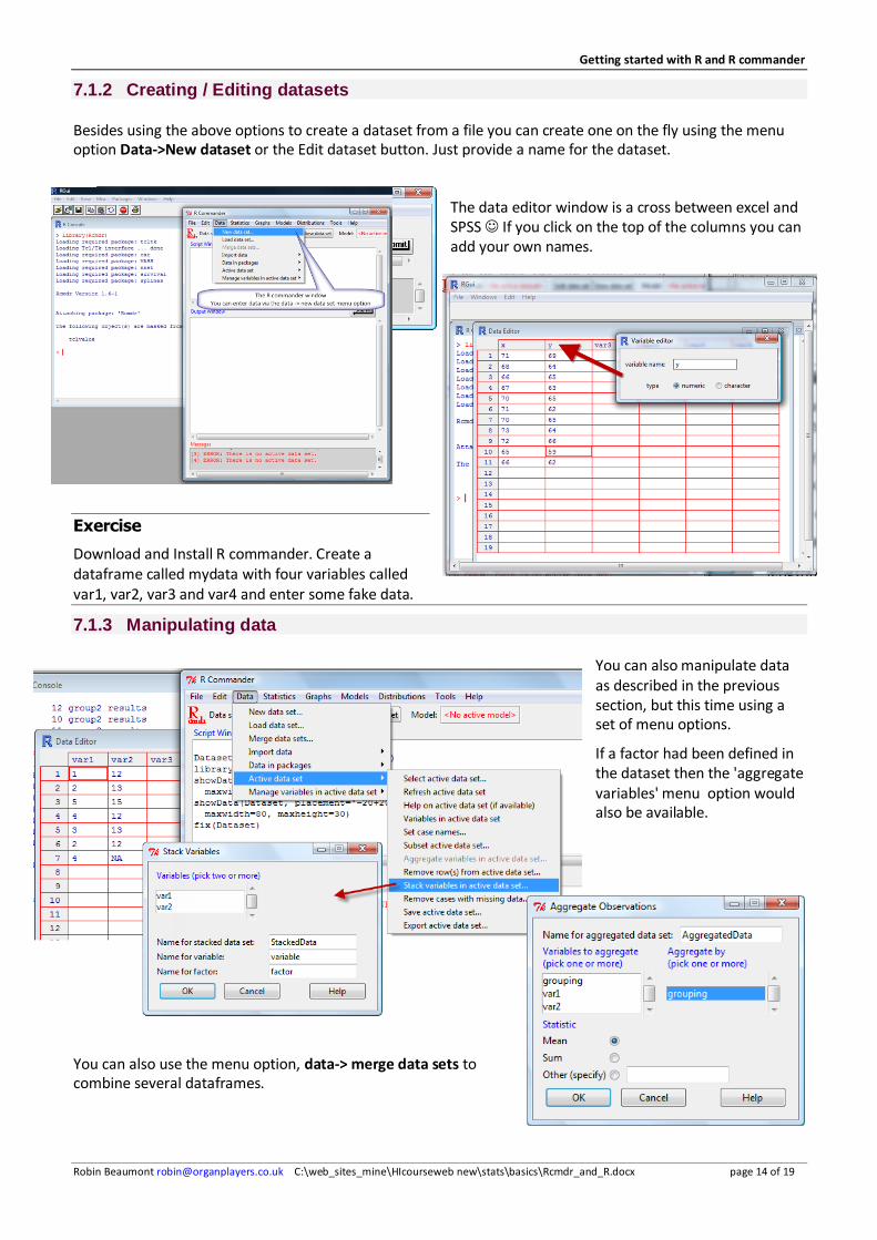
7.1.2 Creating / Editing datasets

Besides using the above options to create a dataset from a file you can create one on the fly using the menu option Data->New dataset or the Edit dataset button. Just provide a name for the dataset.

The data editor window is a cross between excel and SPSS If you click on the top of the columns you can add your own names.

Exercise

Download and Install R commander. Create a dataframe called mydata with four variables called var1, var2, var3 and var4 and enter some fake data.

7.1.3 Manipulating data

You can also manipulate data as described in the previous section, but this time using a set of menu options.

If a factor had been defined in the dataset then the 'aggregate variables' menu option would also be available.

You can also use the menu option, data-> merge data sets to combine several dataframes.



7.1.4 Saving Data

For saving data R commander offers you several menu options, The screenshot opposite shows you what to select to save the active dataset as a *.rda data file. You can also select the menu option Data->Active dataset->Export active dataset to allow you to save the active dataset as a text file (commonly called cvs file), under the bonnet R commander uses the write.table command discussed earlier.

7.1.5 Descriptive statistics

You can obtain basic descriptive statistics and plots by using the two following menu options:

You can also produce Histograms, scatterplots, bar graphs etc. using menu options.

Correlations and p values are also available under the Statistics-> summaries menu (see opposite).



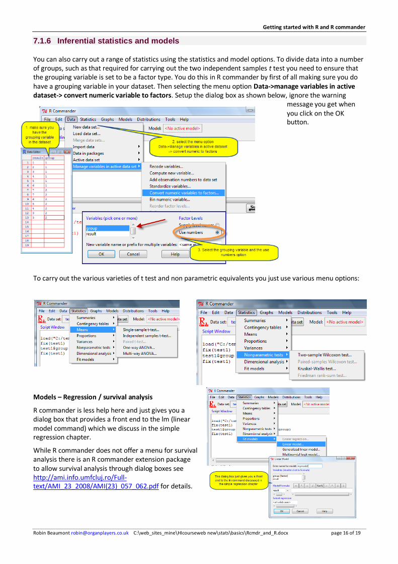
7.1.6 Inferential statistics and models

You can also carry out a range of statistics using the statistics and model options. To divide data into a number of groups, such as that required for carrying out the two independent samples t test you need to ensure that the grouping variable is set to be a factor type. You do this in R commander by first of all making sure you do have a grouping variable in your dataset. Then selecting the menu option Data->manage variables in active dataset-> convert numeric variable to factors. Setup the dialog box as shown below, ignore the warning

message you get when you click on the OK button.

To carry out the various varieties of t test and non parametric equivalents you just use various menu options:

Models – Regression / survival analysis

R commander is less help here and just gives you a dialog box that provides a front end to the lm (linear model command) which we discuss in the simple regression chapter.

While R commander does not offer a menu for survival analysis there is an R commander extension package to allow survival analysis through dialog boxes see http://ami.info.umfcluj.ro/Full-text/AMI_23_2008/AMI(23)_057_062.pdf for details.

http://ami.info.umfcluj.ro/Full-text/AMI_23_2008/AMI(23)_057_062.pdf

http://ami.info.umfcluj.ro/Full-text/AMI_23_2008/AMI(23)_057_062.pdf



7.1.7 Intelligent menus

You will discover, or may have already noticed, that the R commander menu only offers options that are appropriate to the dataset, for example if there is no factor (grouping) variable in the dataframe then no options involving the analysis of groups, such as the Mann Whitney U or two samples independent t test will be available but greyed out. Similarly if there is only one numerical variable in the dataframe then the paired t test will not be offered.

7.2 Deducer

Deducer is more complex to install as it runs under a Java graphical interface called JGR (speak 'Jaguar') which is a universal and unified Graphical User Interface for R. You therefore need to install, java (http://java.com/ ) and JGR before installing Deducer. You can find details of JGR at: http://rforge.net/JGR/screenshots.html

You can find information about JavaGD at: http://www.rforge.net/JavaGD/

install.packages("JavaGD", dependencies=TRUE)

install.packages("JGR", dependencies=TRUE)

install.packages("Deducer", dependencies=TRUE)

My advice to you is to forget it unless you are very computer savvy. The following youtube video may help: http://www.youtube.com/watch?v=J14EJeo4LDU

The analysis menu option provides a few interesting choices:

The dialog boxes that comes up when you select the Two sample test or correlation are shown on the next page:

http://java.com/

http://rforge.net/JGR/screenshots.html

http://www.rforge.net/JavaGD/

http://www.youtube.com/watch?v=J14EJeo4LDU



8. Summary

This short introduction to R and one graphical interface package for, it R commander, has described how you use the application to enter, edit and save data. Each chapter describes the specific commands needed to carry out various detailed analyses.



9. Appendix - Updating R for Windows

This section was taken from the R website at UCLA http://www.ats.ucla.edu/stat/R/ (this link contains a wealth of R related information).

Here are some tips on updating R for Windows.

When you install a new version of R, it is installed in a new directory. This can be a problem because you would need to install all of the packages again.

9.1 Seeing the packages you have installed and their manual installation.

You installed a new version of R, but it does not have many of the packages you had installed in your previous version of R. In fact, you are having trouble remembering the names of the packages you installed. This strategy helps you identify packages that have been installed in your old version of R so you can then reinstall the into your new version of R.

1. Identify the packages you installed in your old version of R

You can see the list of all of the packages you have installed like this. Note this includes the standard packages that come with R as well as ones you installed.

installed.packages()

If you want to just see the first four columns, you can type this

installed.packages()[,1:4]

If you want to see just column 1 and 4 (the package name and it's priority) then you can type this. Packages that have priority of NA are more likely to be ones that you installed.

installed.packages()[,cbind(1:4)]

2. Install packages into your new version of R.

You can install packages into your new version of R by choosing, from the pulldown menu, Packages and then Install Packages from CRAN. You can then look for the package name that you want to install. You can use Ctrl-Click (pressing the control key and left click) to select more than one package at a time for installation.

9.2 Seeing where your packages are installed and copying them all at once

You installed a new version of R, but it does not have many of the packages you had installed in your previous version of R. In fact, you just want to copy over the library directory that you used from your old copy of R to your new copy of R. Here is how you can do that.

Identify the library directory for your old and new version of R. - You can use the .Library command to see where your libraries (packages) are stored. If you install a new version of R, you could execute the .Library command for your old version of R, and your new version of R.

Copy the contents of the library directory from the old version of R to the new version of R - You can then use windows explorer to copy the library directory from your old version of R to your new version R.

Update the packages - It is possible that your old version of R might have had some packages that were out of date, and that you clobbered the newer version. That is OK because you can use the update.packages() function to bring your packages up to date, like this.

update.packages()

If you do not want to be asked about updating each package, you can use the ask=F option, as shown below.

update.packages(ask=F)

http://www.ats.ucla.edu/stat/R/

Date post:	08-Jul-2020
Category:	Documents
Upload:	others
View:	10 times
Download:	0 times

Getting started with R and R commanderGetting started with R and R commander Robin Beaumont...

Documents