1 Getting the Right Fit VMware ESX Workload Analysis SLN056 John Paul – IT Architect, Technology Services Siemens Medical Solutions Health Services [email protected]This presentation has been slightly modified since it was presented at VMworld. Some of the observations and recommendations could have been confusing to the casual reader who did not attend the presentation or read the notes contained herein. I believe that the slight modifications were appropriate and make the presentation more accurate and helpful to our VMware ESX community. Please feel free to contact me with questions and comments. John Paul [email protected]
Transcript
1
Getting the Right FitVMware ESX Workload Analysis
SLN056
John Paul – IT Architect, Technology ServicesSiemens Medical Solutions Health Services
This presentation has been slightly modified since it was presented at VMworld. Some of the observations and recommendations could have been confusing to the casual reader who did not attend the presentation or read the notes contained herein.
I believe that the slight modifications were appropriate and make the presentation more accurate and helpful to our VMware ESX community. Please feel free to contact me with questions and comments.
� With special thanks and contributions from:� Bala Ganeshan, Ph.D., Corporate System Engineer
EMC Corporation (presenter of SLN532)� Greg McKnight, IBM Distinguished Engineer
IBM Systems and Technology Group� Rafael Azria, Victor Barra, Christopher Hayes
Siemens Med VMware Development Team� And a few others who have asked to remain
anonymous but have been invaluable by providing input to this presentation
This presentation has been evolving over the past few months as our understanding of the technology has grown. The presentation started out being based upon over 200 slides of information on W2K and Virtualization performance analysis and has continue to morph.
As an intermediate level presentation it is not meant to be totally comprehensive but rather act as a road map with a legend to guide you through the challenge of workload analysis. We strongly encourage you to visit the vendor forums to see what types of tools can be applied to this task asthings are changing very rapidly and the industry’s knowledge of this technology is also growing rapidly.
3
Considerations
� The recommendations and observations made in this presentation are based upon a real world implementation with a heterogeneous application mix.� Combinations of workloads on what is essentially a shared processing environment (I.e., ESX hosts) will result in different amounts of virtualization overhead. � The same application (ex., an ERP system) may have substantially different results when executing on different processor types and infrastructure.
We suggest that you read the accompanying Notes pages to better understand the intent of each slide. It was difficult to condense all of the information into a 50 minute presentation while still including all of the caveats.
It is difficult to deal in absolutes when doing performance analysis on complex, variable workloads. This presentation was intended to provide real world experience to the attendees and subsequent readers.
We believe that the information in this presentation is accuratefor our environment but strongly recommend that you do your own due diligence when analyzing your own workloads in your own environments.
4
A Basic Approach� Categorize your workload from an architectural perspective� Measure/calculate your current physical and virtual infrastructure capacity � Identify and correct current problems� Determine what are and are not good candidates for virtualization� Design a tiered VMware ESX infrastructure � Apply a litmus test to your design before implementation� Build your tiered VMware ESX infrastructure� Load your virtual containers aiming initially for a low guest machine/server
ratio� From existing servers using P2V, PowerP2V
� Initial resource allocation based upon physical consumption � With new workloads
� Initial resource allocation based upon categorization of server� Measure performance of ESX workloads
As can be expected, this is all about data gathering and analysis. VMware ESX stores its data in basically one area (Proc Nodes) but analyzes it from a variety of angles, which results in inconsistent information. Couple this with the inconsistency of some of the data gathered within the guest machine due to clock drift and the analysis becomes challenging.
This presentation is describing one approach that can be used to analyze the data and apply the results. There are other techniques that would also work but we are sharing what have successfully used in our international network.
5
Before We Get Too Far…
� Think about the workloads in terms of the “Core Four” resources� CPU� Memory� Network (I/O)� Disk (I/O)
� Now Add the Fifth Core Four resource – Virtualization Overhead� ESX is very efficient at handling CPU/Memory but not I/O
� I/O is intercepted in most cases, resulting in increased use of CPU cycles� The faster the I/O (e.g., network) the more virtualization overhead� The more alike the guest machines, the higher the memory sharing� The more often you take sample data, the more overhead on the system
� The analysis may be causing more pain then the root cause
The ability to analyze the workload characteristics of the Windows operating system has been available for several years. Unfortunately many people have not been forced to do an in-depth analysis of those workloads since the workloads were constrained by the limitations of a physical server. When the server became too constraining an upgrade was done to the next “largest” server, often over provisioning what was really needed.
Virtualization has brought us back to the needed due diligence of workload analysis and management, forcing us to look in a fresh way at the Core Fore (plus the new Virtualization overhead) resources.
6
Existing Versus New Workloads
� Existing “real” workloads (on physical servers)� Can be measured for the Core Four resources � Memory and CPU usage may be reasonably calculated for virtual servers� I/O usage can be measured and new I/O infrastructure designed
� These workloads may act substantially different when virtualized!� Different timing between functions� Interaction with other guest machines on the same ESX host
� New workloads are put directly on virtual servers� Unlikely to get sufficient details from vendors for good design� Vendors tend to “aim high” for capacity planning� Vendors are still uncomfortable with virtual solutions� Best to put on staging/swing servers
� Isolates potential problems from existing loads� Simplifies measurement� Allows for deliberate introduction into production farms� Aim initially for a low guest machine/host ratio and increase as the workload
becomes familiar
It is necessary to separate workloads into the two categories of existing and new. A “One Size Fits All” approach does not work well for these two types of workloads.
Existing workloads can react quite differently on a virtual server due to the sharing of system resources and new timing because of virtualization. The overhead of standard management tools that are installed on the guest machines can now have a marked impact on the health of the overall virtual farm. For example, a 10% overhead for asset management and monitoring on a physical server that was underutilized may not be noticeable but when that server is virtualized the cumulative effect could be disastrous. New workloads don’t carry any baggage, but may take a sizeable effort to assess.
7
Architectural Categorization - Web Layer
� HTTP, HTTPS processing � Memory and CPU resource consumption is relatively light unless TCP
sockets are constantly created and released� Network I/O is the top resource consumer � Most files are usually static except for log files� High amount of memory sharing� Target ratio of 12-16 guest machines per quad host � Single CPU allocation� Average memory allocation of 384-500MB of RAM
The Web Layer can be one of the best layers to virtualize from a memory and CPU resource perspective. Network I/O overhead comes back to what type of bandwidth was designed into the network (I.e, 100MB versus a 1-2GB backbone). The effects of a 1GB NIC on the ESX host machine could be significant.
This layer is effectively a static set of files, hence the high amount of memory sharing.
� Memory and CPU resource consumption is VERY high� Low amount of memory sharing within Java Virtual Machines since
memory segments are unique� Target ratio of 4-8 guest machines per quad achieved for our
heterogeneous J2EE workload� Increase the amount of CPU shares allocated� Some workloads work best using SMP� Average memory allocation of about 1-2GB of RAM per guest� Configure JVMs to be leaner� Tuning of JVM heap size and garbage eating cycle is key
� Make sure that the application server returns unused memory to the OS� Heap size should be less then allocated memory, otherwise OS is starved
The web/app layer has proven to be problematic for virtualization due to the Java Virtual Machine unique memory pages. The Idle Memory Tax function of VMware, where the system steals back allocated but unused memory pages, does counteract this problem but then has some effect on the start-up of the JVM once it has more work to do.
The safest approach for this layer is still to allocate sufficient memory to the application server (ex., WebSphere) and then focus the efforts on fine tuning its performance. Be particularly focused on the heap size settings, garbage eating timings, and the maximum number of HttpSession objects based upon the amount of data stored per object.
9
Architectural Categorization – Application Layer
� Essentially batch processing� Resource consumption based upon application but can be
artificially throttled with ESX share settings� This layer can potentially consume all of the ESX host
resources during peak periods� Disk I/O is often the constraining factor� Data drives typically largest for this layer, which requires a
careful analysis of the LUN sizes (if SAN) and LUN performance
� Target ratio of 8-12 guest machines per quad host based upon types of workloads
� Symmetric Multi-Processor allocation is often necessary
This layer can range anywhere from fairly light resource use to fully consuming all resources on the ESX host. This is probably the easiest layer to manage through the prudent use of resource shares allocation.
Load testing is particularly important for this layer. Executing a load test and comparing increased processor shares versus an SMP implementation is time well spent.
10
Architectural Categorization – Database Layer
� DBMS software (e.g., Microsoft SQL Server) is primary consumer� Database may reside on external SAN or local disk� Only consider this for very light database use in ESX 2.5� Disk and network I/O overhead are constraining factors� Substantial virtualization degradation (25-35%) can occur� Target ratio of 1-4 guest machines per quad host � Memory allocation of at least 1GB per guest� Symmetric Multi-Processor allocation IS necessary
The use of virtualization for heavy production database use does not appear to be viable with ESX 2.5. Database access often consumes heavy I/O, both in the disk and network areas, which incur the largest virtualization degradation. The use of virtualization for this layer should limited to development and low load databases at this time.
Note that the major DBMS do take advantage of SMP processing so that is the most efficient way to implement processor allocation for this layer.
� Peak resource periods do not adversely affect functions� Target ratio of 12-16 guest machines per quad host � Memory allocation of 384-512 MB per guest� Single CPU allocation per guest
� File servers� Target ratio of 8-12 guest machines per quad host � Memory allocation of 384-512 MB per guest� Single CPU allocation per guest
� DHCP, DNS, Domain Controllers� These are not good candidates for virtualization if your network is
busy and the expected hit rates for these controllers is high� Test these thoroughly with load tools before deploying� If you do virtualize these, put them lower in the priority list
The non File Server infrastructure servers are prime candidates for virtualization. They do not consistently consume large amount of resources and if their resource use goes up the end user usually is not aware of any impact to their work.
Datacenter Best Practices strongly recommend against virtualization of DHCP, DNX, and Domain Controllers due to their high network I/O resource consumption and vital role in the network infrastructure. Balance this with common sense and a good understanding of the load on these controllers. Note that VMware initially recommended against virtualizing these components and now, after more experience, confirm that they are candidates for virtualization.
12
Good Candidates for Virtualization� “Lightweight” tiers such as web and print servers that only need a system
(i.e., c:) drive� Environments that are destructive at the operating system level so they
cannot be in a shared mode� Multiple copies of essentially the same environments� Environments that need quick and painless partial or full resets of
environments are needed� Systems that can tolerate some degree of performance degradation (e.g.,
Infrastructure Servers)� Servers that are totally under your control� Servers used by groups that embrace change
There are several good candidates for virtualization with a highlikelihood for success. The first obvious candidates are current workloads that have low resource consumption. The infrastructure servers are the next best candidates, which surprises many people, followed closely by testing and light load development environments.
Be careful of development environments since they often are single tiered with all of the layers on a single physical or virtual server image.
13
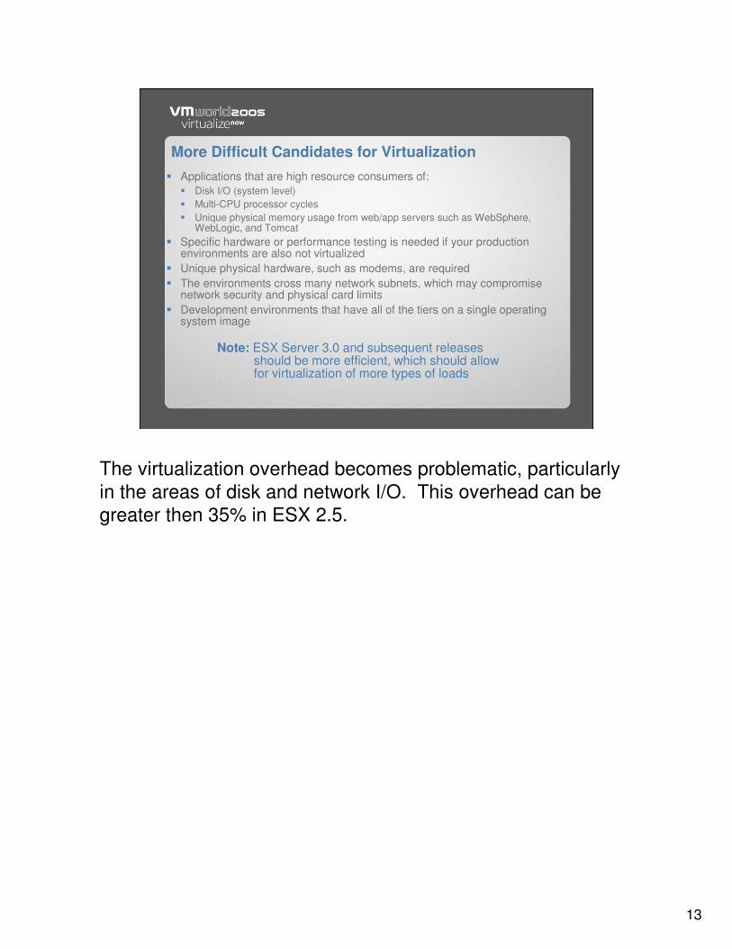
More Difficult Candidates for Virtualization� Applications that are high resource consumers of:
� Disk I/O (system level)� Multi-CPU processor cycles� Unique physical memory usage from web/app servers such as WebSphere,
WebLogic, and Tomcat� Specific hardware or performance testing is needed if your production
environments are also not virtualized� Unique physical hardware, such as modems, are required� The environments cross many network subnets, which may compromise
network security and physical card limits� Development environments that have all of the tiers on a single operating
system image
Note: ESX Server 3.0 and subsequent releases should be more efficient, which should allow for virtualization of more types of loads
The virtualization overhead becomes problematic, particularly in the areas of disk and network I/O. This overhead can be greater then 35% in ESX 2.5.
14
Capacity Testing OverviewThe goal is to establish a physical server baseline for the Core Four � Identify repeatable workloads that can be used to test capacity� Create simple application workloads using automated testing script
engines such as Mercury Load Runner, CompuWare Q.A. Load � Logon, sleep, logoff� Logon, navigate, sleep, navigate, sleep, logoff
� Focus on each architectural layer to validate resources consumedand target virtualization guest machine/host ratio
� Create I/O baseline using a focused tool such as Iometer� Modify Outstanding I/O Per Second, using 1, 8, 16 as targets� Modify LUN Size, Hipers, block sizes
� W2K default block Size is 4K� VMFS block size is 1MB� Some SANs have large blocksize “sweet spots” so ask your SAN
vendors for specifics on your storage solutions� Test both the aggregate throughput of the storage solution as well as the
capacity of the individual paths (ex. FA, front-end CPUs)
The use of load testing tools to do controlled load and capacitytesting is a key to avoiding system melt-downs. The automated tests are used to drive the system infrastructure past its limits to see which component fails and the effect on the other components.
In the I/O realm IOMETER is a good, freeware tool that allows for the controlled testing of the I/O subsystem (both network and disk). This subsystem is one of the first places to look when there are performance issues. Most I/O related performance problems can be eliminated before they happen with good design based upon existing and future workloads.
Local disk can be measured using standard W2K performance tools while SAN and NAS solutions require much more elegant tools and analysis.
15
Core Four Focus Points
� CPU� Average and peak usage per CPU (based upon processor speed)
� Memory� Average and peak memory usage
� Network I/O per NIC � Bytes Total/sec, Packets/sec
� Disk I/O per physical disk� Identify any files that need to support a high I/O per second rate
(such as log files) and consider putting them on fast storage� Identify the average and peak I/O per second rate for the following
types of I/O using native system tool like SysMon/PerfMon� Random read (need multiple spindles on SAN to improve this
I/O)� Random write � Sequential read (pre-fetch caching helps this I/O)� Sequential write (typically used for logs, which are critical path)
This presentation focuses heavily on I/O measurement since I/O has the largest impact on many workloads and incurs the most virtualization overhead. Network I/O is typically best tested and diagnosed with outboard Network Sniffer tools since local tools severely degrade the performance of the operating system image.
Disk I/O should be broken down into the four types of I/O since the I/O subsystem responds differently to each type. The disk I/O analysis should be performed when the average sec/transfer approaches or exceeds 20 ms.
16
Using Iometer for Disk Capacity Testing – File Server
This is a representative load for a file server, based upon Vmware’s experience.
The main window shows each of the accesses that the worker will execute. The first line, for example, shows that 10% of the accesses are 512B, are 80% reads, and 100% random. Other settings in IOMETER specify the duration of the test, as well as output files (a text file), and number of workers and systems.
17
Using Iometer for Disk Capacity Testing – Web Server
This is a representative load for a web server, based upon Vmware’s experience.
The main window shows each of the accesses that the worker will execute. The first line, for example, shows that 22% of the accesses are 512B, are 100% reads, and 100% random. Other settings in IOMETER specify the duration of the test, as well as output files (a text file), and number of workers and systems.
Remember that any load simulation tool such as IOMETER, does not represent actual workloads so results can be skewed, Use these tools carefully as a means to test the capacity of the infrastructure pipes, and then measure actual workloads.
18
ESX NTFS Local Disk
Native W2K NTFS Local Disk
ESX Raw SAN Disk
Native W2K RAW SAN Disk
ESX NTFS SAN Disk
Native W2K NTFS SAN Disk
ESX NTFS Local Disk
Native W2K NTFS Local Disk
ESX NTFS SAN Disk
Native W2K RAW SAN Disk
ESX NTFS SAN Disk
Native W2K NTFS SAN Disk
Blocking Factor - Access 4k - Random Read 4k - Random Write 4k - Sequential Read 4k - Sequential Write
8k - Random Read 8k - Random Write 8k - Sequential Read 8k - Sequential Write
32k - Random Read 32k - Random Write 32k - Sequential Read 32k - Sequential Write
64k - Random Read 64k - Random Write 64k - Sequential Read 64k - Sequential Write
I/O Second MB R/W per second
Sample Disk I/O Performance Grid
This is a performance grid that compares the disk I/O performance of Native (I.e., non-virtualized) W2K versus W2K on ESX for different storage options. It is particularly helpful when establishing a performance baseline that was outside of the variable workloads. We also varied the block size since this directly affects the utilization of the front-end SAN CPU. If re-blocking has to occur, then that CPU located on the SAN frame adaptor is doing the work. Older SANs had very slow front-end CPUs, which caused I/O queuing delays.
I/O Second I/O SecondGB Read/Written GB Read/Written
Disk I/O Performance Grid with I/O Problem
This is a sample only and not intended to be taken as representative of performance numbers.
The previous grid is extended to include relative performance percentages. The number of outstanding I/Os was set to 1, which removed some of the design strengths of the SAN. The local disks were able to out perform the SAN (which is expected) for certain I/Os, while others performed significantlybetter when placed on SAN.
This type of analysis is invaluable when designing the placement of the various files for guest machines and ESX hosts.
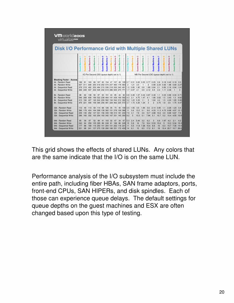
I/O Per Second (OIO (queue depth) set to 1) MB Per Second (OIO (queue depth) set to 1)
Disk I/O Performance Grid with Multiple Shared LUNs
This grid shows the effects of shared LUNs. Any colors that are the same indicate that the I/O is on the same LUN.
Performance analysis of the I/O subsystem must include the entire path, including fiber HBAs, SAN frame adaptors, ports, front-end CPUs, SAN HIPERs, and disk spindles. Each of those can experience queue delays. The default settings for queue depths on the guest machines and ESX are often changed based upon this type of testing.
21
Is There a Current Problem?� Every environment has a bottleneck at some level� Bottlenecks do not always indicate a problem to be corrected� Don’t let the amount of performance data intimidate you!� Build a consistent process to identify problems� Answer some simple questions first
� Are end users reporting a system/application performance problem?� Do the high level system indicators show a problem?
� What does an optimized server look like?� Has sufficient memory to buffer most read and write data so LAN requests almost
never have to wait for disk I/O to be completed� LAN transfers at rated speed will happen without delay/queueing� Disk utilization will typically be low� Processor utilization will be moderate
There is always a current problem or performance bottleneck, the question is where is it and is it in the place that has the least effect on the overall performance?
22
Identifying Current Problems Using PerfMon� If you suspect or have a current performance problem
� Repeatable – use real-time PerfMon monitoring� Sporadic – use tracing until problem is narrowed down
� PerfMon Hints � Beware of Averages and Clock Drift
� Usually displays averages instead of peaks� Maximum means maximum of the averages� Use Current Counters to eliminate smoothing effect� Start at a high level and work your way “down”
� CPU: Processor time for each CPU� Memory: Page Reads/sec, Page Writes/sec� Physical Disk (for each disk): Avg. sec/transfer� Network Interface: Bytes Total/sec, Packets/sec
� Look at Report summary instead of the Chart View� Look at average and maximum values
System Monitor/Performance Monitor is an effective tool for doing some performance analysis but it is not comprehensive, nor accurate in all cases under ESX. Clock drift due to the inconsistent presentation of the clock interrupt to the guest machines does invalidate certain results, while others that are actual counts are still valid.
Use PerfMon as a tool along with other tools in the performance suite. For ESX (mentioned later in this presentation), also use esxtop and Virtual Center, as well as VMkusage and VMKTREE.
23
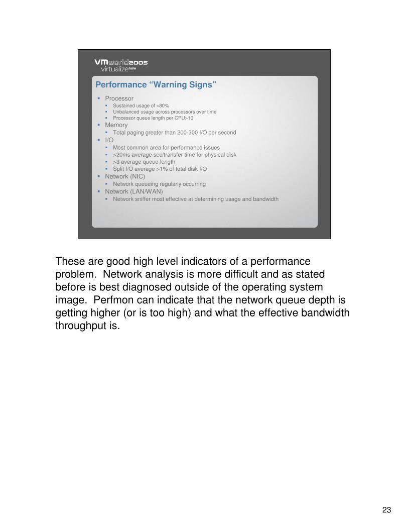
Performance “Warning Signs”� Processor
� Sustained usage of >80%� Unbalanced usage across processors over time� Processor queue length per CPU>10
� Memory� Total paging greater than 200-300 I/O per second
� I/O� Most common area for performance issues� >20ms average sec/transfer time for physical disk� >3 average queue length� Split I/O average >1% of total disk I/O
� Network (LAN/WAN)� Network sniffer most effective at determining usage and bandwidth
These are good high level indicators of a performance problem. Network analysis is more difficult and as stated before is best diagnosed outside of the operating system image. Perfmon can indicate that the network queue depth is getting higher (or is too high) and what the effective bandwidththroughput is.
24
Considerations When Building an ESX Infrastructure � CPU
� The faster the better to overcome virtualization overhead� Memory
� Aggregate physical memory usage -20% memory sharing savings for like workloads� Disk I/O (local storage)
� Contains ESX files so delays are propagated to all guest machines� Choose type of RAID deployment carefully
� RAID Ratio of performance for comparing RAID strategies:� %Reads * (Physical Read Ops) + %Writes * (Physical Write Ops)
� RAID-10, RAID-1, RAID 0+1, RAID-1+0� Two physical disk writes per logical write request are required� I/O Performance = % Read * (1) + % Write * (2)
� RAID-5� Four physical disk I/O operations per logical random write request are required
(two reads and two writes)� I/O Performance = % Read * (1) + % Write * (4)
� Disk I/O (Network or SAN storage)� Largest expected area of disk consumption and expense� Most likely area of performance degradation if not designed correctly
� Include a staging/swing server to hold new workloads
These are some Best Practices to consider when building an ESX infrastructure. The use of a staging/swing server for new loads is highly recommended. That server can also be used as a place to move (via VMotion) performance problems so they can be analyzed.
25
Building a Tiered ESX Infrastructure
� ESX host hardware considerations� Processing demands for single guest machine drive dual or quad choice� Avoid large (8-way or greater) systems due to poor price performance ratios
of larger systems� Memory capacity key (2-4GB per CPU in ESX host)� Local disk capacity is not as important� Deploy multiple hosts of the same processor family for VMotion� Bundle NICs whenever possible to avoid single point of failure� Build a migration strategy for technology refreshes
� SAN Storage considerations� High virtualization overhead area for ESX if disk I/O rates are high� ESX places unique demands on storage (all down one “pipe”)� Use multiple fiber HBAs for SAN� Manually assign different HBAs to guest machines since automatic load
balancing is not yet an ESX option� Spread I/O across multiple frame adapters and front end CPUs� Separate workloads into high I/O per second requirements and then design
storage solutions appropriately. Do not design only by capacity.
There are many ways to build an ESX infrastructure. The long term intent for the farm is key in deciding how much to invest in the underlying infrastructure (network and storage). A localdisk-only approach does work but the lack of VMotion is so detrimental that at some point the operations staff will demand to go to a network solution. Hopefully additional ESX support for lower cost options will be available in the not too distant future.
We have found that the larger (8-way or above systems) have such a high price point as to not be cost effective, which is why we are currently recommending using quad processors.
26
Storage Strategy� Consider a multi-tiered storage strategy, based upon both
capacity and performance needs� Local Disk� NAS� SAN
� Design the SAN for performance at a LUN level and not just an aggregate throughput level across the SAN� Individual guest machines usually operate on a single LUN
� Set preferred path to enable some level of load balancing acrossHBAs using vmkmultipath –s xxx –r xxx command
� Use a tool such as IOMETER to create a I/O baseline on existing storage and compare that baseline against virtualized server I/Operformance
Each storage solution, in and of itself, has its own problems and challenges. Local disk does not allow for Vmotion or redundancy, but is the cheapest storage solution. NAS is not currently supported by ESX (until 3.0) but can be used for file shares for the guest operating systems. SAN provides the most robustness but is much more expensive then the other solutions, particularly if you use an enterprise SAN solution.
A tier solution leverages the strengths of each of the storage options. Make sure that your solution tests single path performance as well as aggregate path since ESX does not have multi-pathing support.
27
SAN Storage Strategy Matrix
� Multiple VMFS allows more VM’s per ESX server.� Response time of limited concern (can optimize)
� Limited # of VM’s due to response time issue.� Limited # of IO intensive VM’s since one VMFS
Scalability
Functionality
Performance
Management
� Use VMFS when storage functionality not needed.� Judicious use of RDM vs. VMFS
� All VM’s share one LUN.� Cannot leverage ALL available storage
� Can result in poor response time.� No manual load balancing
� Slightly harder management.� Storage provisioning has to be on demand.� One VMFS to manage (spanned)
� Easier management.� Storage can be under provisioned.� One VMFS to manage.
Storage as multiple LUNsStorage as single LUNs
This is a good summary slide that came from Bala’s presentation that is referenced earlier. The decision on which size LUN, how many LUNs, which servers access each LUN has to be done with operational simplicity in mind. From a performance perspective a 100GB LUN is best but that causes problems with the limitations on the number of LUNs that can be accessed within a farm and the operational challenges of managing that many LUNs.
An approach of a standard performing farm with larger LUNs and a high performing farm with smaller LUNs should be considered.
28
A Litmus Test for an Example Configuration � Current physical processor configuration for our example farm
� 6 dual processor 500 MHZ, 1 GB RAM, web servers� 25% average, 50% peak CPU utilization� 6GB system drive, no data drive� 350MB average, 500MB peak, memory utilization
� 2 dual processor, 1GHz, 1GB, web/app servers� 25% average, 100% peak CPU utilization� 6GB system drive, no data drive� 350MB average, 1GB peak, memory utilization
� 4 quad processor, 750MHz, 1GB, application servers� 25% average, 75% peak CPU utilization� 6GB system drive, 20GB data drive� 350MB average, 750MB peak, memory utilization
� 4 dual processor, 750MHZ, 1GB, infrastructure servers� 25% average, 50% peak CPU utilization� 6GB system drive, 20GB data drive, high I/O usage� 350MB average, 500MB peak, memory utilization
It is often best to bring points home via examples. Before any implementation is done a litmus test needs to be conducted to make sure that any solution is within the bounds of reasonableness. This example allows us to work through one type of litmus test. The servers listed above are physical servers, with the indicated utilizations.
29
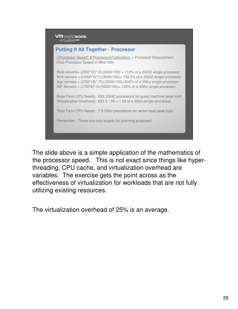
Putting It All Together - Processor((Processor Speed* # Processors)*utilization) = Processor RequirementHost Processor Speed in Mhz/100)
Web servers= ((550*12)*.5)/(3000/100) = 110% of a 3GHZ single processorW/A servers = ((1000*4)*1)/(3000/100)= 133.3% of a 3GHZ single processorApp servers = ((750*16)*.75)/(3000/100)=300% of a 3Ghz single processorINF Servers = ((750*8)*.5)/(3000/100)= 100% of a 3Ghz single processor
Base Farm CPU Needs: 633.3GHZ processors for guest machine peak loadVirtualization Overhead: 633.3 *.25 = 1.58 of a 3Ghz single processor
Total Farm CPU Needs: 7.9 3Ghz processors for worst case peak load
Remember: These are only targets for planning purposes!
The slide above is a simple application of the mathematics of the processor speed. This is not exact since things like hyper-threading, CPU cache, and virtualization overhead are variables. The exercise gets the point across as the effectiveness of virtualization for workloads that are not fullyutilizing existing resources.
The virtualization overhead of 25% is an average.
30
Putting It All Together – Memory and Storage(Total Memory * Utilization) - 10-20% memory sharing = Memory use
Total disk space: (6*36) + (2*6) + (4* (6+20)) + (4*(6+20)) = 1880GB
In a manner similar to the processing slide, we can estimate the needed memory and storage needs based upon the current loads. A 20% memory sharing savings is a reasonable average based upon experience.
Note that these estimates do not indicate HOW to deploy the solution but rather how much resource is needed for a solution.
31
Putting It All Together – What Works for You� Dual versus quad processor ESX hosts
� Existing available hardware versus net new buy� Scalability of ESX host hardware
� Expected growth of each workload� Is the the end of just the beginning of the complex?� Expect the word to spread that virtualization is a reality
� Existing infrastructure that can be leveraged for this implementation� Net new SAN implementations are very expensive� Watch out for ESX/VC storage limitations (ex., 128 LUN limit)
� List your operational and performance priorities and service level expectations
Many configurations will work. Get your financial team involved!
Now that you have the resources required you need to look at the financial perspective for implementation. Many configurations will work well, but some could be hundreds of times more expensive then others. Let the financial and asset management team get involved.
Note that the foundational building block of either a dual or quad processor ESX host has become the de facto standard for many users. SMP usage tends to move the solution to quads for many workloads. Consider the number of ESX hosts and the current limitations for Virtual Center support.
32
Performance Monitoring under ESX
� Monitor at different levels and perspectives to get the “whole story”� W2K Guest Machine
� System Monitor/Perfmon and Task Manager� ESX
� Virtual Center� Management Console� VMktree and VMkusage
� Console Operating System� ESXtop
� Different monitors will show different results� Timer interrupt inconsistent� Different sampling rates (like measuring the height of a camel)
Let’s move on to the actual performance monitoring under ESX. There is no single tool available from VMware that gives you the comprehensive interactive and trend performance analysis for all ESX implementation components. Again we recommend you look at the Vendor Forum to see what is now available or in their plans.
We do want to recommend the use of a tool such as Virtual Center, that allows you to look at the overall ESX landscape. This view is invaluable for operating medium to large ESX farms and is the starting place for performance monitoring.
33
Virtual Center – Disk I/O Weekly Range
Virtual Center gives a good trend Core Four view of either the ESX host(s) or the guest operating systems. The visual representation quickly points out major performance issues.
Once a performance issue is noticed then you need to turn to other tools for more granularity as to what is actually happening. Virtual Center has by default a large sampling interval, which means it could easily miss spikes of resource consumption. The sampling approach is normal for operating systems to avoid huge degradation for monitoring.
34
Management Console – Memory Sharing Example
The ESX Management Console provides a lower level view of specific resource consumption, including a good visual diagram of the memory utilization and sharing. It is a good exercise to launch this view after an ESX host is rebooted and watch the ESX kernel go through the memory sharing process.
In the example above you can see the amount of memory that is in the shared pool and the overall benefits of memory sharing.
35
VMKTREE – Top LUN IO Usage
VMKTREE is a good tool to use to drill down on any performance issue. It pulls data from the same source as VMKusage (which can be launched from VMKTREE). This is a tool that you should become very familiar with and review the system trends on a weekly basis.
36
ESXTOP
ESXTOP is best launched from an SSH session and gives a unique, interactive view of all system resources. The first line (which is cropped here) should look like:
12:10 PM up 32 days 2:12, 10 worlds, load average:
The second line (also cropped) is Physical CPU (PCPU)
This view has hyper-threading enabled so it shows LCPU, Memory, Swap File, Disk (physical disk) utilization, NIC utilization
VCPUID (virtual CPU ID), WID (World ID), Wtype (world type),
%Used (by VCPU), %Ready (VCPU ready to run but cannot),
%EUSED (Effective % of Processor used by VCPU), %MEM (% of memory used by VCPU)
Use lower case F to toggle fields
37
Conclusions and Recommendations
� Find tools that you are comfortable with and learn them well� Keep watching for new tools since they are coming quickly� Do proactive monitoring of existing workloads� Stay active with local user groups and boards� Go to every session you can at VMworld since there is much
information to be gathered. There is overlap on sessions but this reinforces best practices from both VMware and end users.
� Develop a repeatable process for workload analysis� Share your experiences and knowledge with others� Virtualize, virtualize, virtualize whenever possible
Let’s move on to the actual performance monitoring under ESX. There is no single tool available from VMware that gives you the comprehensive interactive and trend performance analysis for all ESX implementation components. Again we recommend you look at the Vendor Forum to see what is now available or in their plans.
We do want to recommend the use of a tool such as Virtual Center, that allows you to look at the overall ESX landscape. This view is invaluable for operating medium to large ESX farms and is the starting place for performance monitoring.