196
Gianni Amisano Carlo Giannini Topics in Structural VAR Econometrics 2nd edition
| Date post: | 17-May-2018 |
| Category: |
Documents |
| Upload: | nguyenkien |
| View: | 215 times |
| Download: | 1 times |

Gianni Amisano Carlo Giannini Topics in Structural VAR Econometrics 2nd edition

iv
Gianni Amisano Carlo Giannini Dipartimento di Dipartimento di Economia Scienze Economiche Politica e Metodi Quantitativi Università di Brescia Università di Pavia Via Porcellaga, 21, via S. Felice, 5 25121 Brescia, Italy 27100, Pavia, Italy [email protected] [email protected]

v
To Anne, Vittoria and Andrea

vi

vii
Foreword In recent years a growing interest in the structural VAR approach
(SVAR) has followed the path-breaking works by Blanchard and Watson (1986), Bernanke (1986) and Sims (1986), especially in the U.S. applied macroeconometric literature. The approach can be used in two different, partially overlapping, directions: the interpretation of business cycle fluctuations of a small number of significant macroeconomic variables and the identification of the effects of different policies.
SVAR literature shows a common feature: the attempt to "organise", in a "structural" theoretical sense, instantaneous correlations among the relevant variables. In non-structural VAR modelling, instead, correlations are normally hidden in the variance-covariance matrix of the VAR model innovations.
VAR analysis tries to isolate ("identify") a set of independent shocks by means of a number of meaningful theoretical restrictions. The shocks can be regarded as the ultimate source of stochastic variation of the vector of variables which can all be seen as potentially endogenous.
Looking at the development of SVAR literature we felt that it still lacked a formal general framework which could embrace the several types of models so far proposed for identification and estimation.
This is the second edition of the book, which originally appeared as number 381 of the Springer series "Lecture notes in Economics and Mathematical Systems". The author of the first edition was Carlo Giannini.
The second edition is a revised and augmented version of the first one, where the additional parts focus on a series of issues and developments in the econometric literature, and are motivated by the many questions addressed to the author of the first edition by different researchers. These issues were developed and discussed within a research group including Rocco Mosconi (Dipartimento di Economia e Produzione, Politecnico di Milano), Mario Seghelini (Research Unit, Deutsche Bank, Milan) and the two authors of this second edition.
In our view, it is very difficult to attribute most of the new parts of the book specifically to any of the two co-authors. Nevertheless,

viii
the absolute majority of the new parts originate from the contribution of the new co-author, who has largely benefited from the material and the results contained in his Ph.D. thesis.
The second edition of this book is justified, beside the fact that the first one was sold out, by the many developments in VAR econometrics, especially in cointegration analysis, which rendered the previous edition of the book inadequate, since it just contained some summary indications in that respect. We felt that it was necessary to discuss all the methodological and practical issues connected to the application of the Structural VAR framework to cointegrated settings.
Moreover, we had to take into account the problem raised in a series of papers by Marco Lippi, Lucrezia Reichlin and Danny Quah, and related to the existence of non fundamental representations. In this book we discuss at length the relevance of this problem, in the light of the existing literature, and we present a new method, based on the estimation of VARMA models, of checking whether the validity of the dynamic simulations obtained from a structural model is affected by the relevance of non fundamental representations. Nevertheless, we believe that on this problem other work will be necessary. Appendix D of the first edition has been eliminated from the second edition. This appendix contained the description of two RATS (written by Antonio Lanzarotti and Mario Seghelini) performing the estimation and the dynamic simulation of Structural VAR models. These two procedures, now available at the ESTIMA WWW site (http://estima.com), were not immediately applicable to the analysis of cointegrated systems. For this reason, they have been modified by Gianni Amisano and Mario Seghelini and they are now incorporated as a Structural VAR Analysis menu of the menu driven RATS computer package MALCOLM (MAximum Likelihood analysis of COintegrated Linear Models), written by Rocco Mosconi1 (see Mosconi, 1996) and designed to perform VAR and Structural VAR analysis in possibly cointegrated systems. Most of

ix
the computations described in chapter 9 of this book were performed by using the MALCOLM package. MALCOLM will be available on the Internet at the following URL: http://vega.unive.it/~alex/GRETA/MALCOLM..
The general structure of the second edition of this book is as
follows. Chapter 1 introduces the main concepts of VAR analysis. Following Rothenberg (1971, 1973), chapters 2, 3 and 4 develop
a methodological framework for three types of models (models K, C and AB) which encompass all the different models used in the applied literature. In fact, looking at a selected choice of recent SVAR applied papers one can see the following correspondence with regard to the categorisation put forward in this book: Blanchard and Watson (1986) is an example of K-model; Blanchard and Quah (1989) and Shapiro and Watson are examples of C-models; Bernanke (1986) and Blanchard (1989) are examples of AB-models.
We have also tried to generalise the identification and the estimation set-up by using the most general type of linear constraints available for the representation of beliefs on the organisation of instantaneous responses of the endogenous variables to "exogenous" independent shocks.
Building on Lütkepohl (1989, 1990), chapter 5 contains calculations of the asymptotic distributions of impulse response functions and of forecast error variance decompositions. In this chapter, we also describe the possibility of using bootstrapping or Monte Carlo integration techniques. Section 5.3 was written by Antonio Lanzarotti.
Chapter 6 includes deals with the treatment of deterministic components, long run constraints in a stationary context, and gives a detailed account of how to use Structural VAR analysis in the presence of (possibly) cointegrated series: In order to do that it was necessary to discuss at length the inferential and modelling issues arising in the presence of cointegration.
In chapter 7 we explain how to use the dominance ordering and the likelihood dominance criteria introduced by Pollack and Wales (1991) as model selection devices in Structural VAR analysis, in order to choose among alternative structuralisations of the same unstructured VAR model.

x
In chapter 8, we describe how to cope with the problems induced by the relevance of non fundamental representations.
Chapter 9 tries to offer deeper insights into SVAR modelling by providing the results of two applied exercises carried out on Italian data sets by using AB-models.
Annex 1 deals with the notion of structure in SVAR modelling, while Annex 2 contains our point of view on the meaning of each of the three types of models discussed in this book. We also try to suggest some criteria on which model to choose in different applications together with some general considerations on their overall working.
Appendix A briefly summarises rules and conventions of matrix differential calculus adopted in this monograph.
Appendix B contains the calculation of the first order conditions for the maximisation of the likelihood of the K-model and the corresponding Hessian matrix.
Appendix C has been written jointly by Antonio Lanzarotti and Mario Seghelini and it contains some examples of symbolic identification analysis for the K, C and AB models.
We wish to thank Fabio Canova, Lorenzo Cella, Riccardo Cristadoro, Carlo Favero, Jack Lucchetti, Massimiliano Serati, Ken Wallis and Sanjay Yadav for useful discussions, and Mario Faliva for providing useful algebraic references. We are also indebted to S. Calliari, J.D. Hamilton, M. Lippi, J.R. Magnus, H. Neudecker, R. Orsi, P.C.B. Phillips, D.S.G. Pollock, H.E. Reimers and to the unknown Springer referee, for their suggestions and encouragements after reading the first version.
Special thanks are due to Antonio Lanzarotti and Mario Seghelini, both for their contributions and for their suggestions. They have accompanied us through a journey started in a fog of confused ideas.
An important acknowledgement is due to the work of Rocco Mosconi. His superb econometric competence and programming skills are clearly witnessed by the quality of his MALCOLM package, which has been extensively used by the authors in order to apply the techniques documented in this book. Beside that, his scientific support has been crucial in different stages of our work.

xi
Finally, we want to thank our families, to which this book is dedicated.
The usual disclaimer obviously applies. Brescia and Pavia, August 1996.
Contents Foreword vii Chapter 1: From VAR models to Structural VAR models 1 1.1. Origins of VAR modelling 1 1.2. Basic concepts of VAR analysis 2 1.3. Efficient estimation: the BVAR approach 6 1.4. Uses of VAR models 10 1.4.1. Dynamic simulation 10 1.4.2. Unconditional and conditional forecasting 11 1.4.3. Granger causality 13 1.5. Different classes of Structural VAR models 15 1.6. The likelihood function for SVAR models 19 1.7. Structural VAR models vs. dynamic simultaneous equations models 22 1.8. Some examples of Structural VARs in the applied literature 23 1.8.1. Triangular representation deriving from the Choleski decomposition of Σ 24 1.8.2. Blanchard and Quah (1989) long run constraints 24 1.8.3. A traditional interpretation of macroeconomic fluctuations: Blanchard (1989) 26 Chapter 2: Identification analysis and F.I.M.L. estimation for the K-Model 29 2.1. Identification analysis 29 2.2. F.I.M.L. estimation 36 Chapter 3: Identification analysis and F.I.M.L. estimation for the C-Model 40 3.1. Identification analysis 40

xii
3.2. F.I.M.L. estimation 45 Chapter 4: Identification analysis and F.I.M.L. estimation for the AB-Model 48 4.1. Identification analysis 48 4.2. F.I.M.L. estimation 57 Chapter 5: Impulse response analysis and forecast error variance decomposition in SVAR modelling 60 5.1. Impulse response analysis 60 5.2. Variance decomposition (by Antonio Lanzarotti) 67 5.3. Finite sample and asymptotic distributions for dynamic simulations 73 Chapter 6: Long run a priori information. Deterministic components. Cointegration 78 6.1. Long run a priori information 78 6.2. Deterministic components 82 6.3. Cointegration 85 6.3.1. Representation and identification issues 88 6.3.2. Estimation issues 91 6.3.3. Interpretation of the cointegrating coefficients 98 6.3.4. Asymptotic distributions of the parameter estimates: Structural VAR analysis with cointegrated series 100 6.3.5. Finite sample properties 103 Chapter 7: Model selection in Structural VAR analysis 107 7.1. General aspects of the model selection problem 107 7.2. The dominance ordering criterion 108 7.3. The likelihood dominance criterion (LDC) 111 Chapter 8: The problem of non fundamental representations 114 8.1. Non fundamental representations in time series models 114 8.2. Economic significance of non fundamental representations and examples 118 8.3. Non fundamental representations and applied SVAR analysis 120

xiii
8.4. An example 125 Chapter 9: Two applications of Structural VAR analysis 131 9.1. A traditional interpretation of Italian macroeconomic fluctuations 131 9.1.1. The reduced form VAR model 132 9.1.2. Cointegration properties 133 9.1.3. Structural identification of instantaneous relationships 134 9.1.4. Dynamic simulation 135 9.2. The transmission mechanism among Italian interest rates 136 9.2.1. The choice of the variables 136 9.2.2. The reduced form VAR model 137 9.2.3. Cointegration properties 139 9.2.4. Structural identification of instantaneous relationships 143 9.2.5. Dynamic simulation 145 9.2.6. The Lippi-Reichlin criticism 149 Annex 1: The notions of reduced form and structure in Structural VAR modelling 151 Annex 2: Some considerations on the semantics, choice and management of the K, C, and AB-models 154 Appendix A 159 Appendix B 162 Appendix C (by Antonio Lanzarotti and Mario Seghelini) 165
References 174

xiv
1
Chapter 1 From VAR models to Structural VAR models
In this chapter we introduce the philosophy, the basic concepts and definitions of VAR analysis (sections 1.1 and 1.2). After that, in section 1.3 we discuss the problems of VAR estimation and in section 1.4 we describe the possible uses of VAR models. Then in section 1.5 we start dealing with Structural VAR analysis, pointing out the main features of the different classes of Structural VAR models, their likelihood functions (section 1.6) and their differences with respect to the standard simultaneous equations models (section 1.7). We conclude this chapter by providing examples of Structural VARs taken from the applied econometric literature (section 1.8). 1.1. Origins of VAR modelling
Before the last two decades, the traditional econometric analysis used to rely on the specification and estimation of large scale structural simultaneous models, in order to analyse the interactions between sets of macroeconomic variables. Uses of those systems ranged from forecasting to policy analysis and testing of competing economic theories. The research activity conducted by the Cowles Commissions in the United States in the period 1945-1970 was entirely based on such large scale models, whose specification was mainly inspired by theoretical considerations derived from the (then) prevailing Keynesian paradigm.
In the 1970s this approach to macroeconometric modelling came under fierce attack on different fronts. Firstly, the great turbulence of those years and the instability connected to unprecedented events such as the collapse of the Bretton Woods system and the oil shocks led to a widespread forecasting failure of the vast majority of the main macroeconometric models. Secondly, the economic profession started questioning the validity of Keynesian theories, and to advocate the use of models with an explicit treatment of the role of rational agents' expectations, in order to correctly represent the interactions among macroeconomic variables. Overlooking the forward-looking rational behaviour of agents would produce

2
structural models incapable of delivering correct answers to the usual policy analysis exercises.
Thirdly, the specification methodology of large scale macroeconometric models was deeply criticised by C.A. Sims (1980, 1982), who emphasised two different methodological weaknesses: i) the specification of simultaneous equations systems was largely based on the aggregation of partial equilibrium models, without any concern for the resulting omitted interrelations. ii) the dynamic structure of the model was often specified in order to provide restrictions necessary to achieve identification (or over-identification) of the structural form.
Motivated by these criticisms, Sims suggested scrapping Simultaneous Equations Systems altogether, and to use models whose specification had to be founded on the analysis of the statistical properties of the data under study. In fact, Sims suggested to specify vector autoregressions (VARs), i.e. multivariate models where each series under study is regressed on a finite number of lags of all the series jointly considered. Clearly, in a VAR model instantaneous relationships among variables are not accounted for and are "hidden" in the instantaneous correlation structure of the error terms.
Since the original proposal of Sims, VARs have encountered a widespread success: in many research environments they have supplanted traditional Simultaneous Equations Systems and they have proved to be very useful and flexible statistical tools. However, as it will soon become apparent, the main conceptual problem in their use is related to the interpretation of the instantaneous correlations among error terms, and therefore among observable variables. The structural VAR analysis is based on the attempt to give a sensible solution to this problem, based on the imposition of a set of restrictions. These restrictions become testable when they allow an over-identified structure to be obtained.
1.2. Basic concepts of VAR analysis
In order to introduce the basic elements of VAR analysis, let us suppose that we can represent a set of n economic variables using a vector (a column vector) yt of stochastic processes, jointly

3
covariance stationary without any deterministic part and possessing a finite order (p) autoregressive representation.
A(L) yt = εt A(L) = I-A1L-... -Ap L
p The roots of the equation det[A(L)] are outside the unit circle in
the complex domain and εt has an independent multivariate normal distribution with 0 mean.
εt ~ IMN(0,Σ) E(εt) = 0 E(εt εt′) = Σ det(Σ) ≠0 E(εt εs′) = [0] s ≠ t
In other words εt is a normally distributed vector white noise (henceforth VWN).
The yt process has a dual Vector Moving Average representation (Wold representation)
yt = C(L) εt C(L) = A(L)-1 C(L) = I + C1L + C2 L
2 +... where C(L) is a matrix polynomial which can be of infinite order and for which we assume that the multivariate invertibility conditions hold, i.e. det[C(L)] = 0 has all the roots outside the unit circle, so
C(L) -1 = A(L) From a sampling point of view, let us suppose that we have T+p
observations for each variable represented in the yt vector; we are thus able to study the system
A(L)yt = εt t = 1,... T This system can be conceived as a particular reduced form (in which all variables can be seen as endogenous).
In order to relate our discussion to the usual Simultaneous System formulae, this latest system can be re-written in compact form as follows (in relation to more usual Structural Simultaneous System Formulae we are assuming a "transposed" notation):
Y = A1Y-1 + A2Y-2 +... + ApY-p + V or even more compactly:
Y = Π X + V where
Y = [y1, y2,..., yT ] Y has dimension (n ×T)

4
Y-i = [y1-i, y2-i,..., yT-i ] Y has dimension (n×T) V = [ε1, ε2,..., εT ] V has dimension (n × T) Π = [A1, A2,..., Ap ] Π has dimension (n × np) X = [Y-1′, Y-2′,..., Y-p ′]′ X has dimension (np × T) If no restrictions are imposed on the Π matrix, the formulae for
asymptotic least squares estimation and maximum likelihood estimation of Π, say $Π , coincide:
$ ' ( ' )Π = −Y X XX 1
Notice that on the basis of this formula, the estimator $Π is independent of the variance-covariance matrix of the error terms εt.
Under the hypothesis that the elements of yt are stationary, we can assume that
[ ] [ ]plimT
ET
t t t t t t p→∞
− − −= = =XX Q x x x y y y' ( ' ) , ' , ' ,... ' '1 2
where Q is a positive definite matrix. Under the hypotheses introduced, it can be easily shown that
T vec vec Nd
( $ ) ( , )Π Π Σ Π− → 0 where the symbol vec A shall indicate, as usual, the column vector obtained by stacking the elements of the A matrix column after
column, d
→ means convergence in distribution (hereafter we shall use usual asymptotic notations such as the one contained in White, 1984, and Serfling, 1980) and
Σ ΣΠ = ⊗−Q 1 If no restrictions are imposed on the Σ matrix, its maximum
likelihood estimate will be:
$ $ $ 'Σ = ∑−
=T t t
t
T1
1ε ε
where $ $ $ ... $ε = y A y A y A yt t t p t p− − − −− − −1 1 2 2 , or more compactly:
$ $ $ 'Σ = −T 1VV where $ $V Y X= − Π .
A consistent estimate of ΣΠ is given by: $ ( ' ) $Σ ΣΠ = ⊗−T XX 1
5
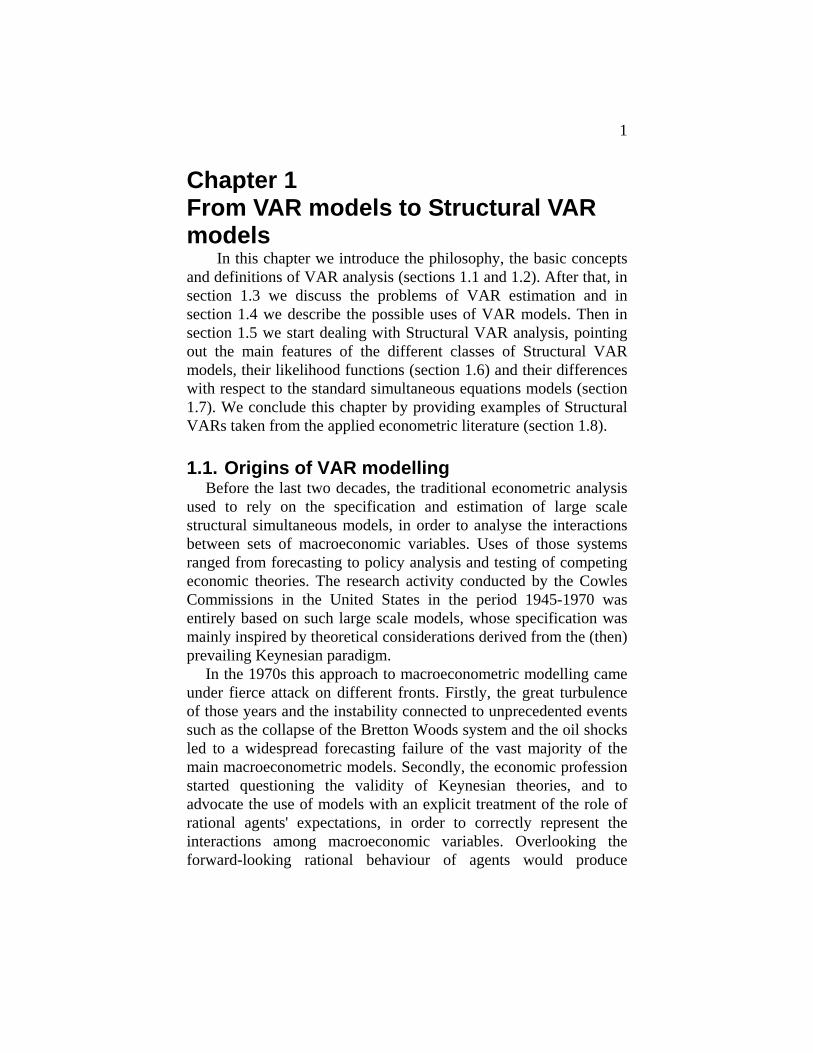
Having estimated the VAR parameters, it is possible to obtain an estimate of the VMA representation parameters, by means of the relationship A(L)C(L)=In. This relationship can be conveniently expressed in matrix terms, by means of the companion form of a VAR(p) system:
zt = A zt-1 + ηt, yt = J zt where:
zt = [yt', yt-1',..., yt-k +1']', ηt = [εt′, 0′]′,
[ ]M
A A A A
I 0 0 0
0 I 0 0
0 0 I 0
J I [0] 0=
⎡
⎣
⎢⎢⎢⎢⎢⎢⎢⎢
⎤
⎦
⎥⎥⎥⎥⎥⎥⎥⎥
−1 2 1...
...
...
... ... ... ... ...
...
... [ ]
k k
n
n
n
, = n
which can be used to obtain the vector moving average (VMA representation) as:
y JM J Cti
t ii
i t ii
k= ∑ = ∑−
=
∞
−=
−'ε ε
0 0
1.
Expression above shows how the VMA parameters can be seen as non linear functions of the VAR parameters. The VMA parameters can be estimated by transformation of the VAR parameters estimates:
$ $ ' ,
$
$ $ ... $ $
...
...
... ... ... ... ...
...
C JM J
M
A A A A
I 0 0 0
0 I 0 0
0 0 I 0
ii
k k
n
n
n
=
=
⎡
⎣
⎢⎢⎢⎢⎢⎢⎢⎢
⎤
⎦
⎥⎥⎥⎥⎥⎥⎥⎥
−1 2 1
The asymptotic distributions of VMA parameters estimates will be described in detail in chapter 5 and 6. In this section we briefly try to convey the intuition behind the available distributional results.

6
VMA parameters are non linear functions of the VAR parameters, and the asymptotic distribution of the OLS estimator of VAR parameters is known. It is then possible to obtain the asymptotic distribution of VMA parameters in the following way. For ease of exposition, let us suppose we have a VAR model of lag order equal to one 1
yt = A yt-1 + εt, εt ~ VWN (0, Σ) In this particularly simple context, the VMA parameters are
Bi = Ai, i = 1, 2,..., and their estimated counterparts are $ $B Ai
i i = , = 1, 2, ... ,
where $A is the OLS estimate of the VAR parameters with the usual asymptotic distribution
( )T vec vec N1 2/ -1 ~ ( , ).$A A 0 Q− ⊗Σ
Now, we consider vecBi as a function of vecA, and we find its first-order Taylor series expansion around vec $A :
-
-
-
vec vecvecvec
vec vec
vec vec
i ii
i j
j
ij
$ ( $ )
( $ ' ) ( $ ) ( $ )
$
B BBA
A A
A A A A
A A
≈ ⎡⎣⎢
⎤⎦⎥
=
= ⊗∑⎡⎣⎢
⎤⎦⎥
=
−
=
−
∂∂
1
1
from which2 it is possible to obtain
( )
( )
- ~
, -1
T vec vec
N
i i
i j
j
ij i j
j
ij
1/2
1
1
1
1
$
( $ ) ( $ ' ) ( $ ' ) ( $ )
B B
0 A A Q A A−
=
− −
=
−⊗∑⎡⎣⎢
⎤⎦⎥
⊗ ⊗∑⎡⎣⎢
⎤⎦⎥
⎧⎨⎩
⎫⎬⎭
Σ
This result conveys the intuition behind the asymptotic distribution of the VMA parameters, which will be discussed in detail in chapter 5.
1 Models with higher dynamics can be treated in exactly the same way. 2 It is easy to see that the terms with order higher than one are asymptotically negligible.

7
1.3. Efficient estimation: the BVAR approach We have already said in this chapter that the maximum likelihood
estimator of the VAR parameters asymptotically coincides with the OLS estimator. The immediate consequence of this fact is that in principle, the estimation of stationary VAR models can be done in a very easy and inexpensive way3, and the resulting estimates are clearly consistent.
In practice though, one of the most serious problems encountered when using VAR models is that these models often have a very high number of free parameters to be estimated. The VAR model has in fact a "profligate parameterization" (Sims, 1980): the number of parameters to be estimated in a VAR of order p is equal to n2 p + n (n +1)/2. For this reason only very small VAR models can be satisfactorily estimated by OLS or maximum likelihood, whereas the VAR analysis of vector series with dimension higher than 5 or 6 is usually precluded by a shortage of degrees of freedom in the typical sample sizes. In such cases, OLS estimates of VARs are typically inefficient, since the sample information is used to estimate a large number of parameters. As a result, the model becomes unreliable for inference in general, and for forecasting in particular.
Since the very start of the VAR literature, this over-parameterisation problem has always been carefully considered. Many different approaches have been proposed in order to obtain more efficient estimates in VAR models. All these approaches, in one way or another, are based on the attempt to constrain somehow the free parameters space4. A particularly successful approach is the use of Bayesian estimation techniques. This approach was first introduced by R. Litterman (1979, 1985) and Doan, Litterman and Sims (1984, henceforth DLS). In this section we briefly describe how the BVAR estimation approach works, and how it can be used to produce more efficient consistent estimates.
3 Things are a bit more complicated in the presence of cointegrated I(1) variables. In such case, the system can also be estimated via maximum likelihood with or without the imposition of the cointegrating rank constraints. For details see chapter 6. 4 See Lütkepohl (1991), chapter 5.

8
In a Bayesian setting, data are not the only sources of information, but they are combined with prior beliefs in order to produce a posterior probability density function (pdf) for the parameters. Imposing these prior beliefs in terms of a prior pdf amounts to somehow constraining the free parameter space, given that the specification of a prior pdf can be seen as the imposition of stochastic (i.e. subject to noise) constraints on the free parameters.
Let us consider the ith equation of the VAR: yit = xt' βi + εit, εit ~ N(0, σi
2) where xt is conveniently defined to include the first p lags of all the variables included in the VAR system.
We call θi = [βi ', σi 2
]' the vector of parameters appearing in the i-th equation. Then, the (partial) likelihood function for the ith equation reads
L(θ|y) = p(y|θ) = (2 π σi 2)-T/2 exp [-(1/2 σi
2) εi ' εi ], εi = [εi1, εi2,..., εiT] '. Classical inference consists in maximising the likelihood
function, in order to obtain an estimate of the parameters. Along with this point estimate, comes an estimate of the associated uncertainty, which is used to construct confidence intervals and to perform hypothesis testing.
The Bayesian approach is radically different: in the Bayesian analysis, there is no such thing as a "true" unknown value of the parameters. On the contrary, these are considered as random unobservable variables, on which the researcher might have some extra-sample (prior) information which is formalised as a "prior" distribution p(θi). Sample and non-sample information are combined by means of Bayes' theorem:
p(θ|y) = p(θ) p(y| θ)/ [∫ p(θ) p(y| θ)d θ ] = p(θ) p(y| θ)/p(y) ∝ p(θ) p(y| θ) The distribution p(θ|y) is called the "joint posterior distribution"
of the parameter vector. This pdf measures the uncertainty on the parameters which results after combining all the sources of available information. This posterior pdf is then used to obtain a point estimate of the parameter vector, usually given by the mode (say $θ ) or the expectation of the posterior pdf.

9
From a different viewpoint, and focusing only on the first order parameters βi, one can think of having prior information about q linear combination of the parameters in the form:
R βi = d + e0, E(e0) = 0, var(e0 e 0') = Σ0 This formulation differs from the usual linear constraints in that
the extra-sample information about βi is subject to error, which implies prior uncertainty.
Considering extra-sample information as q additional observations leads to a feasible GLS mixed estimator
~β i = [ $σ −2 X'X+ R' Σ0
-1 R]-1[ $σ −2 X'y+ R' Σ0-1d], (1.1)
var( ~β )= [ $σ −2 X'X+ R' Σ0
-1 R]-1,
where $σ 2 is any consistent estimate of the i-th equation error terms variance. The expression above corresponds to the well-known Theil-Goldberger (1961) mixed estimator. Litterman (1979) showed that ~
β i is an approximation of the posterior pdf mode, and can be used as a point estimate of the parameter vector.
In order to render the mixed estimation procedure operational, it is necessary to provide a prior distribution for the parameters of the model. In the classical BVAR literature (see for instance Litterman, 1979, 1986, DLS, 1984), the prior is specified taking into consideration that most observed economic time series have long run behaviour similar to that of a random walk process. This remark can be accommodated into a prior distribution framework by requiring that in every equation the parameter on the first lag of the dependent variable is given prior mean equal to one, and all the other parameters are given zero prior mean. This specification of the prior has become standard in the classical BVAR literature and the resulting prior has been termed Minnesota prior 5.
The second moments of the prior distribution are specified on the grounds of two considerations: 1) For easing the computations, the parameters in each equation are assumed as a-priori uncorrelated. In this way, the prior variance-covariance matrix of the parameters is clearly diagonal. 2) As regressors for yit, the own lags of yit are more
5 The term “Minnesota prior” arose because this approach was developed when both Sims and Litterman were at the University of Minnesota.

10
important than the lags of the other elements of the vector yt, and the importance of the single lag decreases with the lag order.
These considerations can be reflected in a prior distribution where the prior variances of the single autoregressive parameters aij,k are devised to become smaller as k increases, and when i≠j. This aim is accomplished in the classical BVAR literature by specifying prior variances according to the choice of a small set of hyperparameters as follows:
[var (aij,k)]1/2= s(aij,k) = γ k- δ f (i,j) σii /σjj, f (i,i) = 1, f (i,j) < 1 for i≠j,
and σii and σjj are the standard errors of the error terms in the i-th and j-th equations. These quantities appear in order to render scale-free the prior variance of aij,k, and in the application of the feasible mixed estimator they must be substituted with consistent estimates (say $σ ii and $σ jj). Calling Σ0 the resulting prior variance covariance matrix, the mixed estimator defined by expression (1.1) can be implemented 6 yielding VAR parameter estimates which are generally more efficient than the usual OLS estimates
The operational simplicity of the Minnesota prior approach is that the prior itself is governed by the choice of a finite set of hyperparameters, which should reflect the intensity of prior beliefs. In the applied BVAR literature though, the hyperparameters cannot be interpreted as reflecting subjective information and their choice is conducted as to optimise the forecasting performances of the model (see for instance DLS,1984)
Therefore, the results of the application of the BVAR procedure are
~( )A L and
~Σ , which are consistent estimates of the auto-
regressive parameters and of the unstructured errors variance covariance matrix. Like the usual OLS or maximum likelihood estimates, these Bayesian estimates can be used as a starting point for the estimation of a Structural VAR. Examples of this procedure are Sims (1986) and Canova (1991).
6 In the BVAR approach it is also possible to specify time varying VAR models, which are then estimated by means of Kalman Filter (see DLS, 1984). These models can be very useful for forecasting purposes, but less indicated for the dynamic simulation purposes typical of SVAR models.

11
1.4. Uses of VAR models
We have already seen that a VAR model is just a reduced form where instantaneous correlations are left uninterpreted. Nevertheless, a VAR model, can be used satisfactorily for a wide range of purposes, which are illustrated in the next three sub-sections. 1.4.1.Dynamic simulation
Imagine that the researcher is interested in the dynamic interactions among the variables in yt, say the effects on yi of a change occurred in yj h periods before. In this case it is possible to refer to the VMA representation of the VAR
yt = C(L) εt and imagine to perturb yjt with a shock εjt equal to one. The effect of this shock on yit+h could then be measured by the VMA coefficient cijh, i.e. the i-th row, j-th column element of the matrix Ch. The problem is that such a measure would not take into consideration the instantaneous correlations existing among the elements of εt and measured by the extra-diagonal elements of Σ. For this reason, it would not be legitimate to perturb one element of εt leaving the others to zero.
Therefore, a VAR model cannot be correctly used for dynamic simulations unless the researcher is ready to provide an interpretation of the instantaneous correlations among the elements of εt. This interpretation is called Structuralisation of the VAR. The issue of how to conduct dynamic simulations with Structural VARs will be analysed in detail in chapter 5. 1.4.2. Unconditional and conditional forecasting
A VAR model can be easily used to generate conditional and unconditional forecasts. From the theoretical point of view, we define the information available at T as the set
IT ={yτ: τ ≤ T} = {ετ: τ ≤ T} It is well known that the optimal linear forecast of yT+h given IT is the conditional expectation

12
y A y C
y y
t h t i t h i ti
p
i t h ii h
T T
+ + −=
+ −=
∞
= =
= ∀ ≤
∑ ∑| |
|
,1
ε
τ τ τ
Hence, the estimated VAR, or its dual estimated VMA representation can be used to obtain consistent estimates of the expressions above as:
$ $ $ $ $ ,
$
| |
|
y A y C
y y
T h T i T h i Ti
p
i T h ii h
T T
+ + −=
+ −=
∞
= =
= ∀ ≤
∑ ∑1
ε
τ τ τ
In this way, the estimated BVAR can be mechanically used to generate unconditional forecasts on the future values of the endogenous variables considered in the model.
This is of course straightforward, but two conceptual problems do arise. First of all, confidence intervals around point forecasts should be provided, in order to explicit the uncertainty connected to the estimation and extrapolation of the model. In principle, since multi-step forecast errors are continuous non-linear functions of the VAR parameters estimates, it is possible to obtain asymptotic distributions for the forecast errors, in the same way as asymptotic distributions can be found for the VMA parameters. Alternatively, finite sample forecast error variances estimates can be obtained numerically, for example resorting to bootstrapping techniques.
Another conceptual problem arises when the researcher wants to forecast conditional on some future values of the endogenous variables. The most appropriate way to consider this problem is to look at the VMA representation, and to imagine that conditioning on some future values of y entails to condition on some future non-zero values of the disturbances ε; in other words, some of the future ε's have to be different from zero in order to generate the future values of the y's which represent the scenario of the forecast. Given the contemporaneous correlation structure of the ε's given by the Σ matrix, it is conceptually inappropriate to impose non zero values to some elements of εT +j, whereas some others are left equal to zero. It is necessary then to work with the orthogonalised VMA representation yt = Φ(L) et, Φi = Ci P, PP' =Σ, et = P-1 εt

13
where P is the Choleski factor of Σ. The forecasts of yT+h, conditioned on the event that some future
values of yT+j, j = 1,..., h, are different from their unconditional forecasts, are then obtained as:
$ $ $|
* *|y e yT h T i T h i
i
h
T h T+ + −=
−
+= ∑ +Φ0
1
where the error terms [ ]e e e eh T T T hvec* * * *, , ...,= + + +1 2 are obtained as the solution of
min ' ,
. . ,e
e e
Re rh
h h
hs t =
and the constraints R eh = r are specified as to generate the scenario of the forecast. In this way, the conditional forecast $ |
*yT h T+ is obtained as an estimate of the projection of yT+h on IT
* = IT ∪YT+h*,
exploiting the contemporaneous correlations among the elements of y as measured by the Σ matrix. 1.4.3. Granger causality
VARs are unrestricted reduced form models, useful as a starting step in order to guide the specification of a fully fledged dynamic structural model. In this light, they are useful devices to analyse causation links among variables, and to guide the researcher in deciding which series, among the observed variables, are truly exogenous.
The concept of causation in econometric models dates back to the contributions of Wiener (1956), and Granger (1969). For a detailed account of the issue of causality in econometrics, it is possible to refer to Geweke (1984).
Imagine to analyse a (n ×1) vector of stationary time series yt, partitioned in two sub-vectors: y1t and y2t with dimensions (n1×1) and (n2 ×1) respectively, n1 + n2 = n. Define
It = { yτ : τ ≤ t }, I2t = { y2τ : τ ≤ t } i.e. It is the information set containing all the past and current values of yt, whereas I2t is the information set containing only the past and current values of y2t.

14
The concept of Granger causation can be described as follows. The vector y1t fails to Granger cause y2t if the predictive density of y2 has the following property
p (y2t+h |It) ≡ p (y2t+h | I2t), ∀ h ≥ 1 which means that conditioning also on the past of y1 does not alter the predictive density of y2. In other words, knowledge of past and current values of y1 does not help to predict future values of y2.
In the case of Granger non causality from y1 to y2, the VAR representation for yt is
A A
0 Ay
0
11 12
22
11 12
21 22
( ) ( )
( ),
( , ),
L L
L
VWN
t t
t
⎡
⎣⎢⎢
⎤
⎦⎥⎥
=
⎡
⎣⎢⎢
⎤
⎦⎥⎥
~ =
ε
ε Σ ΣΣ Σ
Σ Σ
where clearly the block A21(L) is equal to a (n2× n1) matrix of zeroes.
The block-triangular structure of the VAR representation is also retained by the associated VMA representation
yC C
0 CC It t n
L LL
= 0=⎡
⎣⎢⎤
⎦⎥11 12
22
( ) ( )( )
,ε
since the relationship A(L) C(L) = In implies
C I
C A C
0
1
1 2
=
= =−=
∑n
k j k jj
k
k, , , ...
Therefore all VMA coefficient matrices must be block triangular as the VAR matrices.
Also, non causality from y1 to y2 implies that the VAR representation can be transformed by pre-multiplying it by the matrix
A I0 I0
1 12 221
2
=−⎡
⎣⎢
⎤
⎦⎥
−n
n
Σ Σ
The result is the following system
15
A A
0 Ay
00
0
A
11 12
22
11 12 221
21
22
12 12 2210
* **
* * *
*
( ) ( )
( ),
( , ),[ ]
[ ]
( )
L L
L
VWN
t t
t
⎡
⎣⎢⎢
⎤
⎦⎥⎥
=
−⎡
⎣⎢⎢
⎤
⎦⎥⎥
=
−
−
~ =
ε
ε Σ ΣΣ Σ Σ Σ
Σ
Σ Σ
At this point, it can immediate be seen that: a) the error terms of the two blocks of equations are orthogonal b) in the first block of equations, we have also the contemporaneous values of the elements of y2 as regressors for y1t. These two considerations taken together mean that when y1 does not Granger-cause y2, y2 is also strictly exogenous (in the sense of Sims, 1972) with respect to y1.
Clearly, Granger non-causality from y1 to y2 is easily testable, by verifying the joint significance of the parameters in A21(L) in a VAR framework. For the details of this testing procedure, see Geweke (1984).
Some caution in interpreting the results of non-causality tests is necessary. First of all, results are usually very sensitive to the information set being used in the application (i.e. the set of series being included in the VAR): there is always the risk of finding "spurious" causation links deriving from omitted variables. Moreover, in the presence of forward-looking behaviour, Granger causality tests can deliver results which might be at odds with the "true" causation mechanisms driving the behaviour of the variables being analysed7.
1.5. Different classes of Structural VAR models
As we have already stressed, a VAR model has to be considered as a reduced form model where no explanations of the instantaneous relationships among variables are provided. These instantaneous
7 For a simple and very illuminating example of this, see Hamilton, 1994, Example 11.1.
16
relationships are naturally hidden in the correlation structure of the Σ matrix, and left completely uninterpreted.
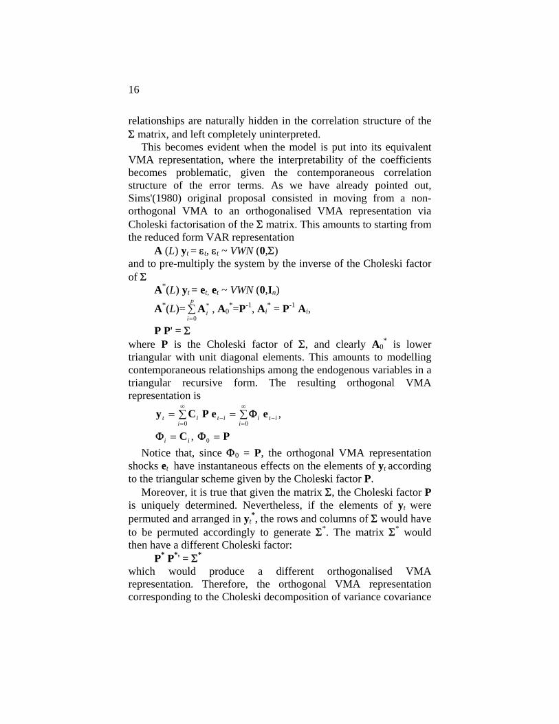
This becomes evident when the model is put into its equivalent VMA representation, where the interpretability of the coefficients becomes problematic, given the contemporaneous correlation structure of the error terms. As we have already pointed out, Sims'(1980) original proposal consisted in moving from a non-orthogonal VMA to an orthogonalised VMA representation via Choleski factorisation of the Σ matrix. This amounts to starting from the reduced form VAR representation
A (L) yt = εt, εt ~ VWN (0,Σ) and to pre-multiply the system by the inverse of the Choleski factor of Σ
A*(L) yt = et, et ~ VWN (0,In)
A*(L)= A ii
p*
=∑
0, A0
*=P-1, Ai* = P-1 Ai,
P P' = Σ where P is the Choleski factor of Σ, and clearly A0
* is lower triangular with unit diagonal elements. This amounts to modelling contemporaneous relationships among the endogenous variables in a triangular recursive form. The resulting orthogonal VMA representation is
y C P e e
C P
t i t ii
i t ii
i i
= ∑ = ∑
= =
−=
∞
−=
∞
, 0 0
0
Φ
Φ Φ
,
Notice that, since Φ0 = P, the orthogonal VMA representation shocks et have instantaneous effects on the elements of yt according to the triangular scheme given by the Choleski factor P.
Moreover, it is true that given the matrix Σ, the Choleski factor P is uniquely determined. Nevertheless, if the elements of yt were permuted and arranged in yt
*, the rows and columns of Σ would have to be permuted accordingly to generate Σ*. The matrix Σ* would then have a different Choleski factor:
P* P*' = Σ* which would produce a different orthogonalised VMA representation. Therefore, the orthogonal VMA representation corresponding to the Choleski decomposition of variance covariance

17
matrix of the reduced form disturbances is unique only given a particular ordering of the observable variables contained in yt.
The triangular representation, which is sometimes referred to as Wold causal chain, is clearly a very particular one which cannot be considered suitable to every applied contexts. Sometimes, the researcher might have in mind different schemes for representing these instantaneous correlations, outside the straitjacket of the triangular structures.
In the recent literature, these alternative ways of modelling instantaneous correlations can be summarised in the following terms. Recent literature on the so-called Structural VAR approach uses different ways of structurising the VAR model. We will discuss three such ways: a KEY model which we will call the K-model, the C-model and the AB-model.
In addition to the hypotheses introduced earlier, for the K-model (KEY model) the following expression will hold: K-model
K is a (n ×n) invertible matrix such that K A(L) yt = K εt K εt = et E(et) = 0 E(et et') = In The K matrix "premultiplies" the autoregressive representation
and induces a transformation on the εt disturbances by generating a vector (et) of orthonormalised disturbances (its covariance matrix is not only diagonal but also equal to the unit matrix In). Contemporaneous correlations among the elements of y are therefore modelled through the specification of the invertible matrix K. The structural K-model can be thought of as a particular structural form with orthonormal disturbance vector.
Note that assuming we know the true variance covariance matrix of the εt terms from:
K εt = et K εt εt' K ' = et et'
taking expectations one immediately obtains KΣK' = In.
The previous equation implicitly imposes n(n+1)/2 non-linear restrictions on the K matrix, leaving n(n-1)/2 free parameters in K.

18
C-model
C is a (n ×n) invertible matrix such that A(L) yt = εt εt = C et E(et) = 0 E(et et') = In In this particular structural model, we have a structural form
where no instantaneous relationships among the endogenous variables are explicitly modelled. Each variable in the system is affected by a set of orthonormal disturbances whose impact effect is explicitly modelled via the C matrix.
Sims (1988) stresses the point that there is no theoretical reason to suppose that C should be a square matrix of the same order as K. If C were a square matrix, the number of independent (orthonormal) transformed disturbances would be equal to the number of equations. Many reasons lead us to think that the true number of originally independent shocks to our system could be very large. In that case the C matrix would be a (n× m) matrix, with m much greater than n. In this sense, this research path is opposite to the one studied by the factor analysis, which attempts to find m (the number of independent factors) strictly smaller than n. The case of a rectangular (n×m) matrix C, with m>n, conceals a number of problems connected with the completeness of the model and the aggregation over agents - see a short and not very illuminating discussion of this topic in Blanchard and Quah (1989). In this book, we will not face this problem and we will assume C square and invertible. Nevertheless, we think that many important issues can be better treated following the research path indicated before.
Turning back to our C model, the εt vector is regarded as being generated by a linear combination of independent (orthonormal) disturbances to which we will refer hereafter as et. This may have a different meaning than that of the K-model, where one is concerned with the explicit modelling of the instantaneous relationships among endogenous variables.
As for the C-model, notice that from εt = C et εt εt ' = C et et ' C '
taking expectations,

19
Σ =C C ' If, again, we assume to know Σ, the previous matrix equation implicitly imposes a set of n(n+1)/2 non-linear restrictions on the C matrix, leaving n(n-1)/2 free elements in C. AB-model
A, B are (n×n) invertible matrices8 such that: A A(L) yt = A εt A εt = B et E(et) = 0 E(et et ') = In In this kind of structural model, it is possible to model explicitly
the instantaneous links among the endogenous variables, and the impact effect of the orthonormal random shocks hitting the system.
Notice that the A matrix induces a transformation on the εt disturbance vector, generating a new vector (A εt) that can be conceived as being generated by linear combinations (through the B matrix) of n independent (orthonormal) disturbances, which we will refer to as et. Obviously this structure might have a different meaning than those of models K and C.
Notice also that the AB-model can be seen as the most general parameterisation nesting the C and K models as special cases. In fact, the C-model can be seen as a particular case of the AB-model, where A is chosen to be the identity matrix, and the K-model corresponds to an AB-model with a diagonal B matrix.
As in the previous case, from A εt = B et A εt εt ′A ′ = B B′
for Σ known, this equation again imposes a set of n(n+1)/2 non-linear restrictions on the parameters of the A and B matrices, leaving overall 2n2- n(n+1)/2 free elements.
1.6. The likelihood function for SVAR models
It is important to note that for any of the three classes of SVAR models described above, the log-likelihood function can be
8 The same argument discussed earlier on the size of the matrix C also applies to the matrix B.

20
considered as a function of Π and Σ. Following Sims (1986), and supposing that there are no cross restrictions on Π and Σ or, in more general terms, that there are no restrictions at all on Π while a set of restrictions are imposed on Σ, the identification and the F.I.M.L. estimation of the parameters of models K, C, and AB can be based on the analysis of the following likelihood function
( )L = - 2
| | -2
c T log T tr
T
Σ Σ Σ
Σ
−
−=
1
1
$
$ $ $ 'VV
which is the log-likelihood concentrated with respect to Π. The estimation of Π corresponding to the concentration of the log-likelihood clearly coincides with the OLS estimator when the log-likelihood is conditioned on the first p observations of the sample. Other consistent estimators would yield asymptotically equivalent results as for the subsequent estimation of the Σ matrix.
From this function, three different log-likelihood functions can be obtained for models K, C and AB by substituting Σ with its expressions in the three different cases: K-model
[ ] ( )L ( ) = + 2
| | -2
'2K K K Kc T log T tr $Σ
remembering that, from KΣK'= In, and taking into account the invertibility of K, we can write
Σ=K-1 K'-1 = (K' K)-1, Σ-1 = K'K log|(K′K)-1| = -log[|K|2]; C-model
[ ] ( )L ( ) = - 2
| | -2
2 -1C C C Cc T log T tr ' $Σ
remembering that Σ=C C', Σ-1 = (C C')-1 = C'-1 C-1
AB-model

21
[ ] [ ]
( )L ( ) = +
2 | | -
2 | | +
-2
2 2A B A B
A B B A
c T log T log
T tr ' ' $− −1 1 Σ
remembering that Σ=A-1BB'A'-1, Σ-1 = A'B'-1B-1A By simple inspection of the three log-likelihood functions
obtained by introducing the respective series of non-linear constraints on the matrices K, C, A and B, we can heuristically understand that, lacking further information, likelihood based estimators for the parameters K, C, A and B cannot be found.
All the sampling information necessary to obtain estimates of Σ is contained in $Σ which will have with probability equal to one n×(n+1)/2 distinct elements. By substituting Σ with its expression in terms of K, C, A and B (depending on the particular SVAR model being specified), we overcome the problem of finding a direct estimate of the n×(n+1)/2 elements in Σ (which in reality was not known). There still remains the problem of estimating n2 parameters for the K matrix in the K model, n2 parameters for the C matrix in the C model, and 2n2 parameters (n2 for A and n2 for B) in the AB-model.
It can be heuristically understood that from the sampling information contained in $Σ at most n×(n+1)/2 functionally independent parameters can be estimated in any of the three models. Without additional information we find ourselves in a typical situation of under-identification.
In general, in the existing applied literature the specification of Structural VAR models has been limited to situations of exact identification of the whole set of parameters. This is achieved by aptly imposing exclusion restrictions. One remarkable exception is given by a RATS routine written by T. Doan in three different versions (1987, 1988, 1989). Doan proposes a complete solution for the estimation of over-identified and exactly identified AB-models, with B diagonal and exclusion restrictions on the off-diagonal elements of the A matrix.

22
The exclusion restrictions and the need for exact identification greatly reduce the practical meaning of the Structural VAR approach for a number of reasons which shall be discussed below. To the best of our knowledge, still in the case of exact identification, two papers have tried to introduce new features. In the first of these two papers, Blanchard and Quah (1989), the C-model is used in a system with two variables, and exact identification is obtained by introducing a homogeneous restriction on the parameters of the C matrix, through an infinite-horizon theoretical constraint. In Keating (1990), instead, the AB-model is used for n = 3, with B diagonal and a set of non-linear restrictions on the off-diagonal elements of the A matrix. These restrictions are derived from a variant of Taylor's (1986) rational expectation model.
In what follows we have tried to solve the problem of identification, estimation and use of K, C, and AB-models with additional linear restrictions of the most general kind, namely
R K dk kvec = for K-model R C dc cvec = for C-model
R A dR B d
a a
b b
vecvec
==
⎧⎨⎩
for AB-model
where the Ri matrices (i = k, c, a, b) have full row rank. To these groups of non-homogeneous linear restrictions written
in implicit form correspond three groups of restrictions written in explicit form (see for example Sargan, 1988):
vec k k kK S s + = γ vec c c cC S s + = γ
vecvec
a a a
b b b
A S sB S s
+ +
==
⎧⎨⎩
γγ
where the Si matrices (i = k, c, a, b) have full column rank and the number of columns is equal to the number of free elements in the respective matrices. The number of rows in the Si is obviously n2
and the number of columns is n2 minus the rows of the corresponding Ri matrix.
The following identities will hold for the Ri, di, Si and si vectors and matrices
Ri Si = [0] [0] is a matrix of appropriate order
23
Ri si = di i = k, c, a, b Following the terminology of Magnus (1988), when di = 0, i = k,
c, a, b, the K, C, A, B matrices are called L-structures (linear structures), whereas when di ≠ 0 they are called affine structures.
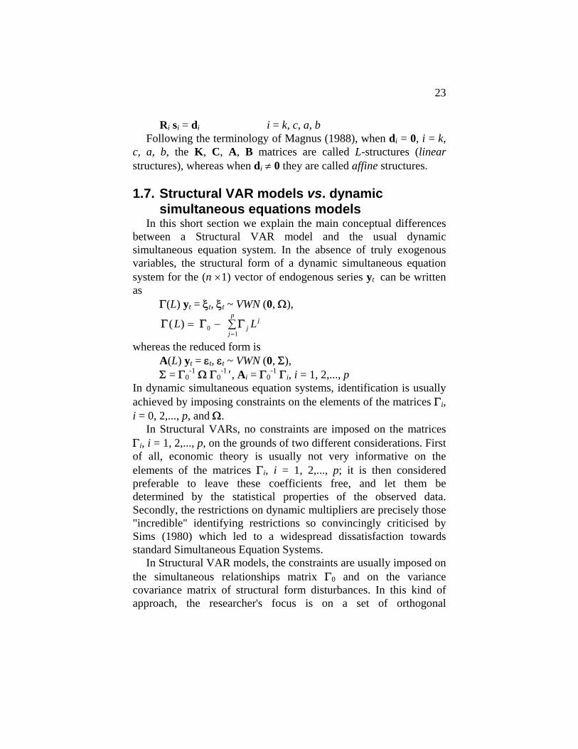
1.7. Structural VAR models vs. dynamic simultaneous equations models
In this short section we explain the main conceptual differences between a Structural VAR model and the usual dynamic simultaneous equation system. In the absence of truly exogenous variables, the structural form of a dynamic simultaneous equation system for the (n ×1) vector of endogenous series yt can be written as
Γ(L) yt = ξt, ξt ~ VWN (0, Ω),
Γ Γ Γ( )L Ljj
pj = − ∑
=0
1
whereas the reduced form is A(L) yt = εt, εt ~ VWN (0, Σ), Σ = Γ0
-1 Ω Γ0-1 ′, Ai = Γ0
-1 Γi, i = 1, 2,..., p In dynamic simultaneous equation systems, identification is usually achieved by imposing constraints on the elements of the matrices Γi, i = 0, 2,..., p, and Ω.
In Structural VARs, no constraints are imposed on the matrices Γi, i = 1, 2,..., p, on the grounds of two different considerations. First of all, economic theory is usually not very informative on the elements of the matrices Γi, i = 1, 2,..., p; it is then considered preferable to leave these coefficients free, and let them be determined by the statistical properties of the observed data. Secondly, the restrictions on dynamic multipliers are precisely those "incredible" identifying restrictions so convincingly criticised by Sims (1980) which led to a widespread dissatisfaction towards standard Simultaneous Equation Systems.
In Structural VAR models, the constraints are usually imposed on the simultaneous relationships matrix Γ0 and on the variance covariance matrix of structural form disturbances. In this kind of approach, the researcher's focus is on a set of orthogonal

24
disturbances, intended as "behaviorally distinct sources of fluctuation" (Sims, 1986, p.9). The structural model is then:
Γ(L) yt = B et, et ~ VWN (0, In), B B′ = Ω and the researcher is willing to impose some constraints on the instantaneous effects of the et on the observable variables yt and on the instantaneous linkages among the endogenous variables.
In synthesis, in Structural VAR models no distinction is drawn between endogenous and exogenous variables, and the constraints are usually imposed on the simultaneous relationships matrix Γ0, which in this book is referred to as A matrix, and on the variance covariance matrix of structural form disturbances Ω, which is parameterised as Ω = B B′. This leads to the structural form
A A(L) yt = B et which represents the typical AB- structural VAR model. The K- and C-models originate as particular cases of the AB-model.
1.8. Some examples of Structural VARs in the applied literature
In this section we present some examples of different SVAR models appeared in the applied literature, in order to help the reader to fully understand the different features of the three classes of Structural Var models. 1.8.1. Triangular representation deriving from the Choleski decomposition of Σ
The triangular representation A*(L) yt = et, et ~ VWN (0,In)
A*(L)= A ii
p*
=∑
0, A0
*=P-1, Ai* = P-1 Ai, P P' = Σ
can easily be interpreted as a K-model, where clearly K = P-1. Since in this case K is by construction lower triangular, we have n(n-1)/2 exclusion restrictions on vecK, corresponding to the elements of K above its main diagonal. This number of restrictions is exactly equal to the number of elements of K which are left free after considering the relationship K Σ K' = In

25
Therefore, in the usual identification jargon, the order conditions for identification would suggest a situation of exact identification (see for details chapter 2).
The recursive VAR corresponding to the Choleski decomposition of Σ can also be interpreted as a C-model A(L) yt = C et, et ~ VWN (0,In) where C = P. Again, since C is lower triangular, n (n -1)/2 exclusion constraints are introduced on C, exactly as many as the elements of C which are left free after considering the relationship Σ = C C' Therefore the usual order condition suggests that this is a case of exact identification of C (see for details chapter 3).
The exact identification of the triangular structure is confirmed by the fact that its estimate can be obtained by applying the Choleski decomposition to $Σ , the estimated variance-covariance matrix of the reduced form disturbances. 1.8.2.Blanchard and Quah (1989) long run constraints
Blanchard and Quah (1989) investigated the dynamic effects of demand and supply disturbances in a bivariate system
yt = Δyu
t
t
⎡
⎣⎢⎤
⎦⎥ = Φ(L) et, et ~ VWN (0,In)
where Δyt is the growth rate of real GDP and ut is the unemployment rate. Both series are stationary and therefore the Wold representation described above exists. The two authors imagine that the first element of et,, e1t, is a demand disturbance which has no long run effect on the level of output. The second disturbance e2t, is considered as a supply shock, which has long run effect on the level of output. These considerations imply the following constraint on the long run structural impulse response function: u1' Φ(1) u1 = 0, where u1' = [1, 0].
The model used by Blanchard and Quah can be interpreted as a C-model where

26
Φ(L) = C(L) C = c L c Lc L c L
c cc c
11 12
21 22
11 12
21 22
( ) ( )( ) ( )
⎡
⎣⎢⎤
⎦⎥⋅⎡
⎣⎢⎤
⎦⎥
and the long-run constraint can be written as c11(1) c11 + c12(1) c21 = 0
In this case, since the relationship Σ = C C' leaves only one free element on the C matrix, the usual order condition suggests that we are in a situation of exact identification9: this intuition is supported by the fact that any C matrix such that10
C C' = Σ can be defined as
C = P Q, Q Q' = Ιn i.e. as an orthonormal transformation of the Choleski factor P.
Defining
C(1) P = D = d dd d
11 12
21 22
⎡
⎣⎢⎤
⎦⎥, Q =
q qq q
11 12
21 22
⎡
⎣⎢⎤
⎦⎥
the C matrix satisfying Blanchard and Quah's long run constraint can be obtained by determining the elements of Q such that
q21 = - d11 q11 /d12 (long run constraint)
q q q qq q
12 21 22 11
112
212 1
= - , =+ =
⎧⎨⎩
(orthonormality of Q)
1.8.3. A traditional interpretation of macroeconomic fluctuations: Blanchard (1989)
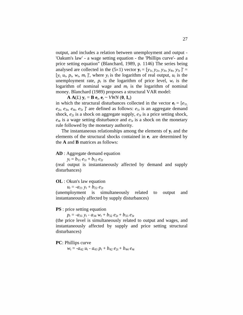
Blanchard (1989) uses the "traditional" Keynesian model to analyse the US macroeconomic fluctuations. by means of a structural AB model, which is intended to capture the main feature of a Keynesian model consisting of aggregate demand, aggregate supply and a monetary rule equation. "Aggregate demand characterizes the behaviour of the aggregate demand for goods given prices. Aggregate supply characterizes the behaviour of prices given
9 The fact that the long run constraint involves the reduced form cumulated impulse response functions coefficients which are not known and must be estimated causes some complications in the Structural VAR analysis. See section 6.1 for further details on this issue. 10 See Blanchard and Quah (1989), p. 657.
27
output, and includes a relation between unemployment and output -'Oakum's law' - a wage setting equation - the 'Phillips curve'- and a price setting equation" (Blanchard, 1989, p. 1146) The series being analysed are collected in the (5×1) vector yt = [y1t, y2t, y3t, y4t, y5t ]' = [yt, ut, pt, wt, mt ]', where yt is the logarithm of real output, ut is the unemployment rate, pt is the logarithm of price level, wt is the logarithm of nominal wage and mt is the logarithm of nominal money. Blanchard (1989) proposes a structural VAR model:
A A(L) yt = B et, et ~ VWN (0, In) in which the structural disturbances collected in the vector et = [e1t, e2t, e3t, e4t, e5t ]' are defined as follows: e1t is an aggregate demand shock, e2t is a shock on aggregate supply, e3t is a price setting shock, e4t is a wage setting disturbance and e5t is a shock on the monetary rule followed by the monetary authority.
The instantaneous relationships among the elements of yt and the elements of the structural shocks contained in et are determined by the A and B matrices as follows: AD : Aggregate demand equation
yt = b11 e1t + b12 e2t (real output is instantaneously affected by demand and supply disturbances) OL : Okun's law equation
ut = -a21 yt + b22 e2t (unemployment is simultaneously related to output and instantaneously affected by supply disturbances) PS : price setting equation
pt = -a31 yt - a34 wt + b32 e2t + b33 e3t (the price level is simultaneously related to output and wages, and instantaneously affected by supply and price setting structural disturbances) PC: Phillips curve
wt = -a42 ut - a43 pt + b42 e2t + b44 e4t

28
(nominal wage is simultaneously related to unemployment and prices, and instantaneously affected by supply and wage setting structural disturbances) MR : monetary rule equation
mt = -a51 yt -a52 ut - a53 pt - a54 wt + b55 e5t (nominal money is simultaneously related to output, unemployment, prices and wages, and instantaneously affected by monetary structural disturbances) For a thorough economic interpretation of these equations, see Blanchard (1989, section II).
The structural VAR model described above has a VAR reduced form
A(L) yt = εt, εt ~ VWN (0, Σ) and the reduced form vector error term εt is related to the structural vector error term et through the set of linear relationships
A εt = Bt et Notice that the structure specified by Blanchard leads to the
following A and B matrices:
A B
1
=
⎡
⎣
⎢⎢⎢⎢⎢
⎤
⎦
⎥⎥⎥⎥⎥
=
⎡
⎣
⎢⎢⎢⎢⎢
⎤
⎦
⎥⎥⎥⎥⎥
0 0 0 01 0 0 00 1 0
0 1 01
0 0 00 0 0 00 0 00 0 00 0 0 0
21
31 34
42 43
51 52 53 54
11 12
22
32 33
42 44
55
aa a
a aa a a a
b bbb bb b
b
,
The two matrices have 17 free elements, while the estimated variance-covariance matrix of the unstructured VAR model disturbances ( $Σ ) contains only 15 different elements. The usual order conditions for identification seems to suggest that the above structure is not identified. For this reason, Blanchard (1989) assigned fixed numerical values to the coefficients a34 and b12. The numerical value given to a34 was derived from previous studies, whereas that assigned to b12 resulted from a sort of calibration reasoning.
Giannini, Lanzarotti and Seghelini (1995) presenting a variant of Blanchard's model applied to Italian data, choose not to set the above mentioned two parameters to fixed constant values, but rather

29
to specify some extra constraints in order to obtain an over-identified structure. For details see section 9.1 of this book.

29
Chapter 2 Identification analysis and F.I.M.L. estimation for the K-Model
In this chapter we present the condition for the identification of the K-model (section 2.1) and we describe how an identified structure can be estimated by means of F.I.M.L. (section 2.2).
2.1. Identification analysis
The K-model1 is completely defined by the following equations and distributional assumptions: K εt = et E(et) = 0, E(et et ') = In εt ~ IMN(0, Σ) det (Σ) ≠ 0 (εt, the vector of the VAR model disturbances A(L)yt = εt is a Gaussian vector white noise, i.e. a vector of independent multivariate normally distributed variables with an associated positive definite variance-covariance matrix).
All the sampling information concerning Σ is contained in the $Σ matrix:
$$ $ '
Σ =VVT
The $Σ matrix can be viewed as the unrestricted estimate of the variance-covariance matrix of the disturbances of the "reduced form": A(L)yt = εt
The corresponding log-likelihood function of the K-model for the parameters of interest (the n2 parameters in the K matrix) is
[ ]L c T T tr( $K K K K) = + 2
log | | -2
( ' ) 2 Σ (2.1)
With respect to this function, the associated density function and the "structural" parameter space, we will assume that the usual
1 Hereafter we will drop the i index (i = k, c, a, b ) to Ri , di , γi , Si , si matrices and vectors unless ambiguity arises.

30
regularity conditions hold, as reported in Rothenberg's (1971) fundamental paper on identification.
The conditions KΣK' = In obviously introduce a set of non-linear restrictions on the parameter space. Therefore, in general, we can obtain only necessary and sufficient conditions for local identification of the parameters in the K matrix as opposed to global identification (see Rothenberg, 1971, p.578).
Moreover, if we are interested only in the joint identification of all K matrix parameters (in the sense of Wegge (1965), we are interested in the identification criteria of a system of equations as a whole) and not in the "isolated" identification of a proper subset of parameters of the K matrix. In Structural VAR Econometrics all the equations of a structuralised VAR are used together, thus "isolated" identification of a proper subset of the parameters in question is of virtually no interest.
In order to achieve identification we will assume that the parameters contained in the K matrix satisfy the set of independent, non-contradictory, non-homogeneous linear restrictions stated in implicit form as follows R vec K = d (2.2) where R is a r×n2 full row rank matrix and d is a possibly non zero r×1 vector, or in explicit form vec K = S γ + s (2.3) where S is a n2×l full column rank matrix with l = n2- r, s is a n2×1 vector and
R S 0
R s d
=
=×
×
[ ]r l
r 1
Following Rothenberg (1971), in order to geometrically analyse the local non-identification situation in the absence of a-priori information contained in (2.2) or (2.3), we will compute the information matrix (the sample information matrix) of the vectorised elements of the K matrix, without taking into account the set of linear restrictions (2.2) or (2.3).
For this purpose we shall compute the vector of partial first derivatives of the log-likelihood function with respect to vec K (the

31
"score " vector) and then the Hessian matrix of the log-likelihood (always with respect to vec K). From this last expression we can then easily compute the sample information matrix.
Taking into account the symbols and notations presented in Appendix A, the score of the likelihood function is (see Appendix B for calculation)2
∂∂
Lvec
f vecK
K= ' ( ) f '(vec K) is a 1× n2 row vector
f vec T T vecr' ( ) ( ) ( )' ( $ ) K K K I= − ⊗−1 Σ or equivalently (see Pollock, 1979), taking into account that (A)r = [vec(A')]' f vec T vec T vec' ( ) [ ( ' ) ]' ( )' ( $ ) K K K I= − ⊗−1 Σ ; obviously the first order conditions for maximisation of the likelihood function are f vec
n n' ( )( )
[ ]( )
K 01 2 1 2×
=×
in row form, or [ ]f vec
nf vec
n n' ( )( )
' ( )( )
[ ]( )
K K 02 1 2 1 2 1×
=×
=×
in column form. Referring again to Appendix A for notation rules and to
Appendix B for calculation, the Hessian matrix of the log-likelihood with respect to vec K is defined as
∂∂ ∂
∂∂
∂∂
2 L L L( )( )'
'
vec vec vec vecK K K K= ⎛
⎝⎜⎞⎠⎟
.
The resulting Hessian can be written as
{H KK K
K K( )( )( )'
( ' )vecvec vec
T
2
= = − ⊗− −∂∂ ∂
L 1 1 OT
+ }$Σ ⊗ I .
2 In order to simplify notation, the In identity (n ×n) matrix will hereafter be substituted simply by I. Identity matrices of different orders will be indicated with their proper corresponding indexes.

32
The sample information matrix of the elements of vec (K) (without taking into account the set of linear restrictions on this vector) has two equivalent definitions for "regular" likelihood functions IT (vec K) = E [-H(vec K)] (*) IT (vec K) = E [f (vec K)⋅ f '(vec K)] (**)
Following (*) and taking into account that E( $ ) ( ' ) ( ' )Σ = =− − −K K K K1 1 1 IT (vec K) = T {[K-1⊗(K')-1] OT +[ K-1 (K')-1] ⊗I} and the properties of the commutation matrix OT (see Pollock 1979 and Magnus 1988) for A, B square matrices of order n (A⊗B) OT = OT ( B⊗A) we can write IT (vec K) = T {(K-1⊗I) OT (K'-1⊗I) + (K-1 ⊗I) (K'-1⊗I) } and finally IT (vec K) = T {(K-1⊗I) ( I
n2 + OT )(K'-1⊗I)}. The corresponding asymptotic information matrix
I (vec K) = plim vecT
T T→∞
1 I K( )
will simply be I (vec K) = {(K-1⊗I) ( I
n2 + OT )(K'-1⊗I)}. The sample information matrix and the asymptotic information
matrix have dimension (n2× n2); it is easily seen however that in our case these matrices are singular, their rank being equal to n(n+1)/2.
Since (K-1⊗I) and (K'-1⊗I) are invertible matrices, the rank of IT (vec K) and I (vec K) is equal to the rank of ( I
n2 + OT ) Using Magnus' (1988) notation and results3, we define: Nn = (1/2)( I
n2 + OT )
obviously4 r(Nn) = r ( In2 + OT ), but Nn is an idempotent matrix5 with
rank n(n+1)/2.
3 See Magnus (1988), p.48. In our notation, the OT matrix replaces Magnus’ Knn commutation matrix.

33
Assuming that the "true" value of the vector of parameters vec(K0) is a regular point of the information matrix IT (vecK) (in the sense of definition 4 of Rothenberg 1971, p.579) and on the basis of Theorem 1 in Rothenberg (1971) which states as the necessary and sufficient condition for the local identification of vec(K0) the non-singularity of IT (vecK0) we can assert, in view of the singularity of IT (vecK) over all the (admissible) parameter space, that vec(K0) is unidentifiable.
In order to get necessary and sufficient conditions for the local identification of the complete vector vecK, we must re-introduce our a-priori information contained in R vecK = d which has thus far been overlooked.
Following Rothenberg (1971) and taking into account that, since these constraint are linear, the Jacobian matrix of the partial derivatives of the system of constraints with respect to vecK is simply R, we can construct the following matrix
VT (vecK)= I KR
T vec( )⎡⎣⎢
⎤⎦⎥
or equivalently
V(vecK)= I KR
( )vec⎡⎣⎢
⎤⎦⎥
The two matrices are of (n2 +r)×n2 order. Following Theorem 2 in Rothenberg (1971) and assuming that
the "true" vector vec(K0) is a regular point (in the sense of Rothenberg) of VT (vecK) and V(vecK), a necessary and sufficient condition for the local identification of vec(K0) is that the rank of VT (vecK) or V(vecK) evaluated at K0 be n2. In other words, the VT (or V) matrices evaluated at vecK0 must be full column rank matrices.
4 As usual, r (A) stands for the rank of matrix A. 5 From the property of the matrix OT : OT ⋅OT = I
n2 .

34
This necessary and sufficient condition is very difficult to verify in our context. Thus, we will try to obtain more tractable conditions which are still absolutely equivalent to those of Rothenberg's Theorem 2 6.
Looking at V(vecK) "augmented" matrix
V(vecK)= ( )(2 )( ' )-1 -1K I N K IR
⊗ ⊗⎡⎣⎢
⎤⎦⎥
n
we can proceed as follows: the rank of V(vecK) is left unchanged if we pre-multiply and post-multiply this matrix by arbitrary non-singular matrices, obviously of the appropriate order.
If V(vecK) is first pre-multiplied by the block diagonal matrix
12 2
( )[ ][ ]
K I 00 I⊗⎡
⎣⎢⎤⎦⎥r
and then post-multiplied by (K'⊗I) the following (n2+r)×n2 matrix is obtained
NR K I
n( ' )⊗
⎡⎣⎢
⎤⎦⎥
Under the condition that (K'⊗I) is invertible (i.e. that K must always be invertible), the matrix above has the same rank as VT and V.
The condition of full column rank (n2) of this matrix is equivalent to the condition that the following homogeneous system of (n2+r) equations in n2 unknowns
NR K I y 0n
( ' ) [ ]⊗⎡⎣⎢
⎤⎦⎥
=
6 In our context IT (vecK), I (vecK) are matrices of constant rank n (n +1)/2 over the admissible parameter space (looking at the information matrix, the admissible space is also constrained by the invertibility of the K matrix). We can heuristically find a necessary condition for identification: taking into account the rank of the matrix IT (vecK), a necessary condition is that it be “augmented” by at least n (n -1)/2 independent rows. In other words, a necessary condition for identification is as follows: r, the number of restrictions on vecK, must be greater than or equal to n (n -1)/2.

35
has only one admissible solution y 0=×
[ ]n2 1
.
The system can be split into two connected systems of equations Nn y = [0] (2.4) R(K'⊗I)y=[0] (2.5) System (2.4) has n2 equations in n2 unknowns. System (2.5) has r equations in n2 unknowns. The two systems are connected because they share the same n2 unknowns.
In order to find closed formulae for the identification analysis we can now proceed in two ways: i) the general solution of system (2.4) is found and inserted in system (2.5) or ii) the general solution of system (2.5) is found and inserted in system (2.4). The former procedure will be followed. The alternative has the advantage of leading to more "parsimonious" conditions for identification, which however are more difficult to interpret.
Considering system (2.4) and looking for the general solution of this system of equations, we will follow Magnus (1988). The vector representing the general solution of system (2.4) can be written as y D x= ~
n where the ~Dn matrix, defined in Magnus (1988), pp. 94-5, is a (n2×n(n-1)/2) full column rank matrix and x is a n(n-1)/2 vector of free elements.
The ~Dn matrix main feature is that for any real valued vector x it generates the vectorised form of a skew-symmetric matrix (say W
( )n n×,
where W = -W') of order n: y = vecW = ~Dn x. We can easily check that this is a solution of system (2.4), remembering the property of the commutation matrix OT : OT vecA = vec(A') for A (n× n) and that for a skew symmetric matrix vec W = -vecW' so for
N In n= +
12 2( OT )
N D x N W In n n nvec~ (= = + 1
2 2 OT )= 12
(vecW+OT vecW)=

36
= 12
(vecW + vecW') = 12
(vecW-vecW) = [0]
This solution is also the general solution by virtue of theorem 9.1 of Magnus (1988), p. 146. Having found the general solution of system (2.4), we can insert it in system (2.5), arriving at R K I D x 0( ' )~ [ ]⊗ =n (2.6) Assuming the invertibility of the K matrix, the necessary and sufficient condition for identification of the "true" vector vec(K0)7 can be wholly derived from system (2.6) and can be stated in two equivalent forms: a) condition for identification
Assuming the invertibility of the K matrix, the true vector vec(K0) is locally identified if and only if the matrix R K I D( ' )~⊗ n evaluated at K0 has full column rank n(n-1)/2. b) condition for identification
Assuming the invertibility of the K matrix, the true vector vec(K0) is locally identified if and only if the system R K I D x 0( ' )~ [ ]⊗ =n with the matrix R K I D( ' )~⊗ n evaluated at K0 has the only admissible solution x=[0].
In practical applications, condition a) can be used and numerically checked remembering to use vecK = S γ +s and assigning "random" numbers to the elements of the γ vector in order to insert an "appropriate" matrix in the (K'⊗ I) nucleus of the formula. The numerical check of the condition does not contribute much to understanding the role and working of different typical constraints.
In Appendix C condition b) is used for the symbolic analysis of a number of interesting cases.
7 Obviously, the “true” vector vec(K0) must satisfy the constraint R vec(K0) = d.
37
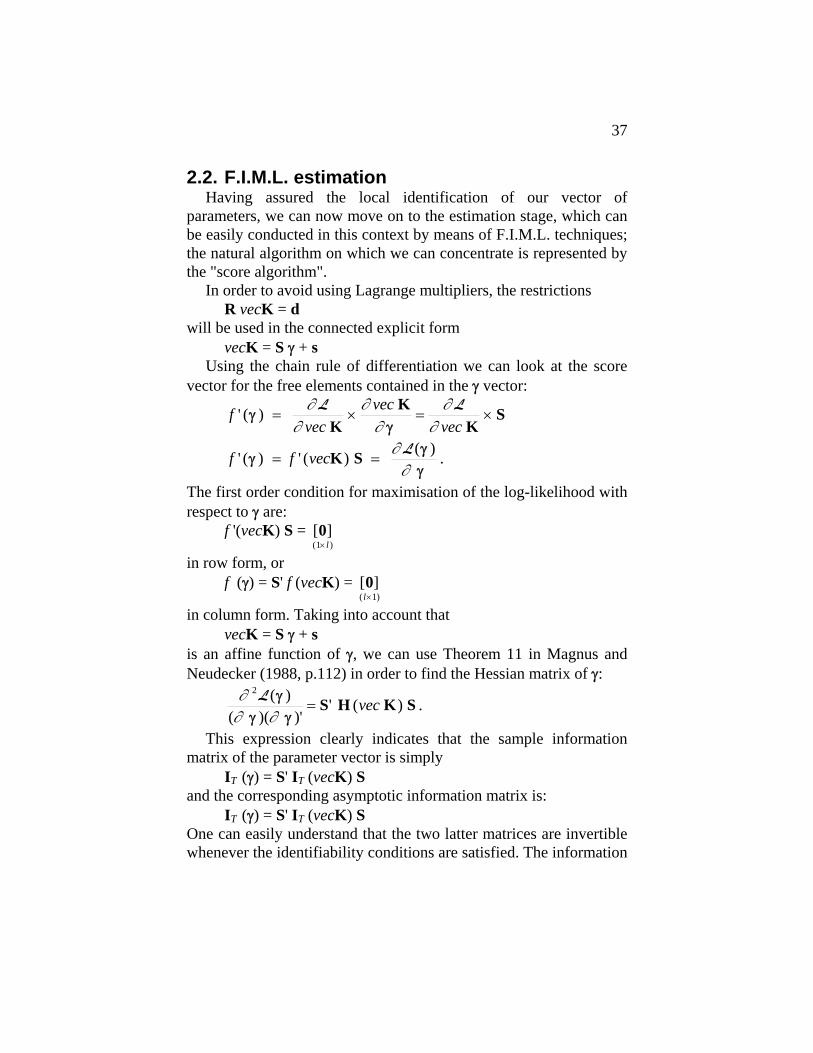
2.2. F.I.M.L. estimation Having assured the local identification of our vector of
parameters, we can now move on to the estimation stage, which can be easily conducted in this context by means of F.I.M.L. techniques; the natural algorithm on which we can concentrate is represented by the "score algorithm".
In order to avoid using Lagrange multipliers, the restrictions R vecK = d will be used in the connected explicit form vecK = S γ + s
Using the chain rule of differentiation we can look at the score vector for the free elements contained in the γ vector:
fvec
vecvec
' ( )γγ
= × = ×∂
∂∂
∂∂
∂L L
KK
KS
f f vec' ( ) ' ( )γγγ
( )
= =K S ∂∂L .
The first order condition for maximisation of the log-likelihood with respect to γ are: f '(vecK) S = [ ]
( )0
1× l
in row form, or f (γ) = S' f (vecK) = [ ]
( )0l×1
in column form. Taking into account that vecK = S γ + s is an affine function of γ, we can use Theorem 11 in Magnus and Neudecker (1988, p.112) in order to find the Hessian matrix of γ:
∂∂ ∂
2L ( )
( )( )'' ( )γ
γ γ= S H K Svec .
This expression clearly indicates that the sample information matrix of the parameter vector is simply IT (γ) = S' IT (vecK) S and the corresponding asymptotic information matrix is: IT (γ) = S' IT (vecK) S One can easily understand that the two latter matrices are invertible whenever the identifiability conditions are satisfied. The information

38
matrix IT (γ) and the score vector f (γ) can be used to implement the "score algorithm" and find a F.I.M.L. estimator of γ (say ~γ ).
Once this vector has been obtained, we can get the F.I.M.L. estimator of vec(K) (say vec ~K ) using vec~ ~K S s= + γ The scoring algorithm for γ is based on the following updating formula (see for example Harvey (1990), p. 134): γn +1 = γn + [ΙT (γn)]-1 f (γn). Choosing the recursion starting values with great care, we can assume a consistent estimate ( ~γ ) of the "true" value (γ0) can be obtained.
Inserting this value in the information matrix we can immediately get the estimated asymptotic variance-covariance matrix of ~γ :
Avar T plimTT
T$ (~ ) (~) (~)γ − γ γ γ= = ⎡⎣⎢
⎤⎦⎥
−
→∞
−
I I111 .
From this matrix, we can get the estimated asymptotic variance-covariance matrix of vec~K via Cramer's linear transformation theorem (see for example Theorem 4 in Sargan (1988), p.5):
[ ]Avar T vec vec$ (~
) (~) 'K K S I S− γ= − 1 ;
under the hypothesis previously introduced, we obviously obtain
~ ( )γ γ, γ ~ AN 1 1
TI −⎡
⎣⎢⎤⎦⎥
and
vec vecT
~( ) 'K K S I S ~ AN , γ
1 1−⎡⎣⎢
⎤⎦⎥
⎧⎨⎩
⎫⎬⎭
Having obtained the F.I.M.L. estimate of vecK, vec~K , we can
re-organise it in matrix form getting the F.I.M.L. estimate of Σ (say ~Σ ). From this matrix and taking into account the expression Σ = (K'K)-1
we can get the F.I.M.L. estimate of the (possibly) restricted variance-covariance matrix of the reduced form disturbances, εt A(L) yt = εt through
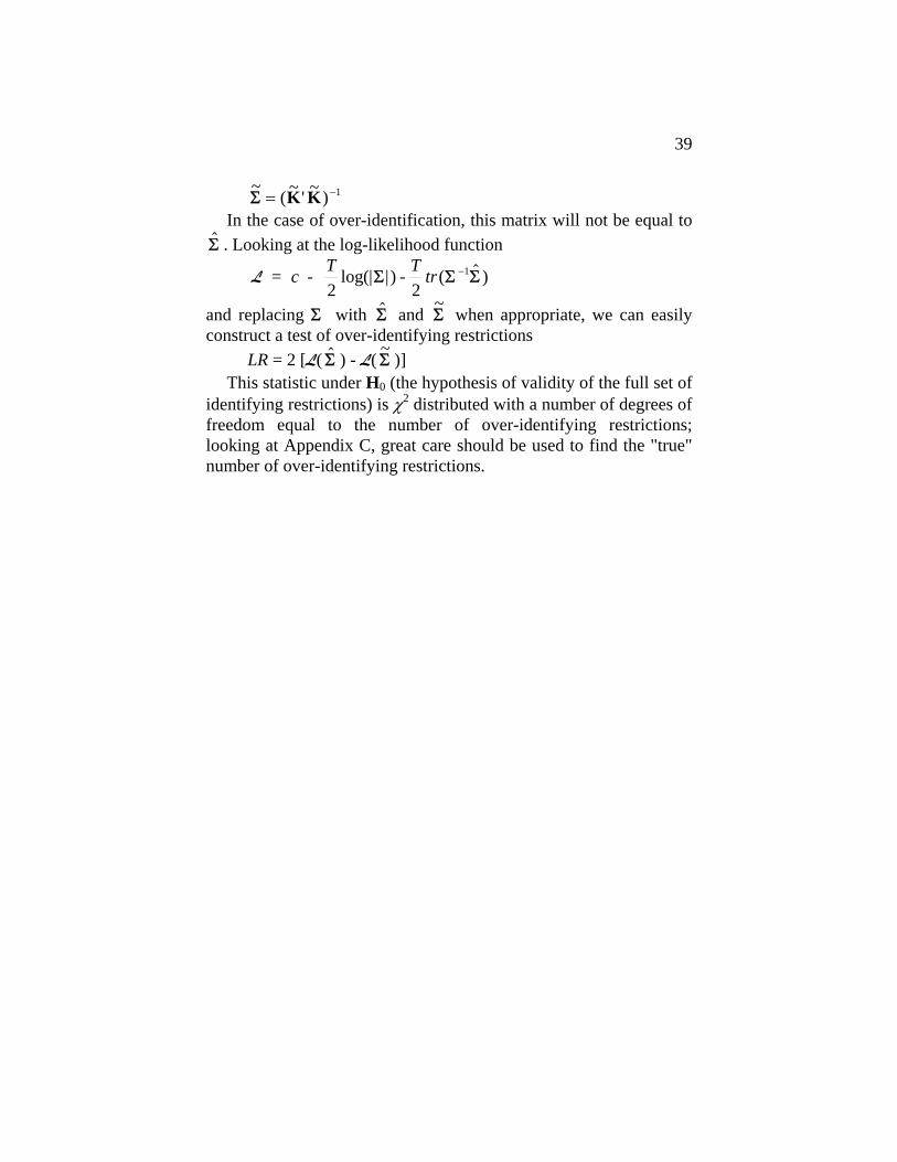
39
~ ( ~ ' ~ )Σ = −K K 1 In the case of over-identification, this matrix will not be equal to
$Σ . Looking at the log-likelihood function
L = - 2
log(| | ) -2
( ) c T T trΣ Σ Σ−1 $
and replacing Σ with $Σ and ~Σ when appropriate, we can easily
construct a test of over-identifying restrictions LR = 2 [L( $Σ ) - L( ~
Σ )] This statistic under H0 (the hypothesis of validity of the full set of
identifying restrictions) is χ2 distributed with a number of degrees of freedom equal to the number of over-identifying restrictions; looking at Appendix C, great care should be used to find the "true" number of over-identifying restrictions.

40
Chapter 3 Identification analysis and F.I.M.L. estimation for the C-Model
In this chapter we present the condition for the identification of the C-model (section 3.1) and we describe how an identified structure can be estimated by means of F.I.M.L. (section 3.2). 3.1. Identification analysis
The C-model1 is completely defined by the following equations and distributional assumptions: εt = C et C square of order n. E(et) = 0, E(et et ') = In εt ~ IMN(0, Σ) det (Σ) ≠ 0 All the sampling information concerning Σ is contained in the $Σ matrix:
$$ $ '
Σ =VVT
where, again, the $Σ matrix can be viewed as the unrestricted estimate of the variance-covariance matrix of the disturbances of the reduced form A(L)yt = εt
The corresponding log-likelihood function of the C-model for the parameters of interest (the n2 parameters in the C matrix) is
L c T T tr( ' $C C C C) = - 2
log(| | ) -2
( ) 2 -1 -1Σ (3.1)
This log-likelihood function can be written as follows
L c T T tr( $C K K K) = + 2
log(| | ) -2
( ' ) 2 Σ (3.1b)
with K = C-1. We assume that all the usual regularity conditions (see Rothenberg, 1971) hold for this function, the associated density function and the "structural" parameter space.
1 Hereafter we will drop the i index (i = k, c, a, b) to Ri , di , γi , Si, si matrices and vectors unless ambiguity arises.

41
The conditions Σ = CC' introduce a set of non-linear restrictions on the parameter space. Therefore, in general, we can obtain only necessary and sufficient conditions for the local identification of the parameters in the C matrix (as opposed to global identification).
In order to achieve identification, we will assume that the parameters contained in the C matrix will satisfy the following set of independent, non-contradictory, non-homogeneous linear restrictions stated in implicit form as R vec C = d (3.2) where R is a r×n2 full row rank matrix and d is a possibly non zero r×1 vector.
In explicit form we have vec C = S γ + s (3.3) where S is a n2×l full column rank matrix with l = n2- r, s is a n2×1 vector and
R S 0
R s d
=
=×
×
[ ]r l
r 1
In order to geometrically analyse the local non-identification situation in the absence of a-priori information contained in (3.2) or (3.3), we will compute the information matrix of the vectorised elements of the C matrix, without taking into account the set of linear restrictions (3.2) or (3.3). Using the chain rule of matrix differentiation and the two equivalent definitions of the information matrix IT (vec C) = E [-H(vec C)]= E [f (vec C)⋅ f '(vec C)] we can by-pass the direct calculation of the Hessian matrix with respect to vecC on the basis of the following considerations.
The score vector of the log-likelihood with respect to vecC can be obtained from the score vector of the log-likelihood with respect to vecK on the basis of the following formula:
∂∂
∂∂
∂∂
L L( ) ( )CC
CK
KCvec vec
vecvec
= ⋅
In fact, remembering that C = K-1, K = C-1 we can write
∂∂
∂∂
L( ) ' ( )CC
K KCvec
f vec vecvec
= ⋅
with
42
( )∂∂ vecvec
KC
C C= − ⊗− −' 1 1
Therefore we have
( )∂∂ L( ) ' ( ) ' .C
CK C C
vecf vec= − ⋅ ⊗− −1 1
But the following relationships also hold IT (vecC) = E [f (vecC)⋅ f '(vecC)] IT (vecC) = (C-1⊗C'-1) E [f (vecK)⋅ f '(vecK)] (C'-1⊗C-1) IT (vecC) = (C-1⊗C'-1) IT (vecK) (C'-1⊗C-1) Remembering the IT (vecK) formula and that C = K-1, it can be shown that IT (vecC) = (C-1⊗C'-1){T (K-1⊗I) ( I
n2 + OT )(K'-1⊗I)} (C'-1⊗C-1) IT (vecC) = T [(I⊗C'-1) ( I
n2 + OT )(I⊗C-1)] I(vecC) = plim vec
TT T
→∞
1 I C( )
I (vecC) = (I⊗C'-1) ( In2 + OT )(I⊗C-1)
The sample information matrix IT(vecC) and the asymptotic information matrix have dimensions (n2×n2), but it is easy to see that up to this point these matrices are singular, their rank being equal to n(n+1)/2.
Since (I ⊗ C'-1) and (I ⊗ C-1) are invertible matrices, the rank of IT (vecC) and I(vecC) is equal to the rank of ( I
n2 + OT ) and equal to the rank of Nn = (1/2)( I
n2 + OT ). We assume that the "true" value of the vector of parameters
(vecC0) is a regular point of the information matrix IT (vecC), in the sense of Definition 4 of Rothenberg (1971). Theorem 1 in the same paper indicates the non-singularity of IT (vecC0) as the necessary and sufficient condition for the local identification of C0. Since IT (vecC0) is singular, then vecC0 is clearly unidentified.
Introducing the constraints R vecC = d

43
and taking into account that, given the linearity of this set of constraints on vecC, the Jacobian matrix of the system of constraints is simply R; following Rothenberg (1971) we can construct the partitioned matrix
VT (vecC)= I CR
T vec( )⎡⎣⎢
⎤⎦⎥
or, equivalently, the matrix
V(vecC)= I CR
( )vec⎡⎣⎢
⎤⎦⎥
These two matrices are of (n2 + r) ×n2 order. Following Theorem 2 in Rothenberg (1971), assuming that the
"true" vector vec(C0) is a regular point (in the sense of Rothenberg's Definition 4) of VT (vecC) and V(vecC), a necessary and sufficient condition for the local identification of vec(C0) is that the rank of VT (vecC) or V(vecC) evaluated at C0 be n2. In other words, the VT or V matrices evaluated at vecC0 must have full column rank.
In order to find more tractable conditions, we shall operate on the "augmented" V(vecC) matrix, exactly as we have done for the K-model. Let us look at V(vecC) "augmented" matrix
V(vecC)=( )(2 )( )-1 -1I C N I C
R⊗ ⊗⎡
⎣⎢
⎤
⎦⎥
' n
It can be first pre-multiplied by the block-diagonal matrix
12 2
( ) [ ][ ]
I C 00 I
⊗⎡
⎣⎢
⎤
⎦⎥
'
r
and then post-multiplied by (I⊗C) arriving at the following (n2+r)×n2 matrix
NR I C
n( )⊗
⎡⎣⎢
⎤⎦⎥
Following the same argument used for the K-model we can look at the system
NR I C y 0n
( ) [ ]⊗⎡⎣⎢
⎤⎦⎥
=

44
trying to discover under which conditions its only admissible solution is y = [0]. The system can be split into two connected systems of equations Nn y = [0] (3.4) R(I⊗C)y=[0] (3.5)
Still by virtue of Theorem 9.1 in Magnus (1988), the general solution of system (3.4) is y D x= ~
n This (general) solution inserted in system (3.5) leads to R I C D x 0( )~ [ ]⊗ =n . (3.6)
Assuming the invertibility of the C matrix, the necessary and sufficient condition for identification of the "true" value2 vec(C0) can be derived looking only at system (3.6) and can be stated in these two equivalent forms: a) condition for identification: assuming the invertibility of the C matrix, the "true" vector vec(C0) is locally identified if and only if the matrix R I C D( )~⊗ n evaluated at C0 has full column rank n(n-1)/2. b) condition for identification: assuming the invertibility of the C matrix, the "true" vector vec(C0) is locally identified if and only if the system R I C D x 0( )~ [ ]⊗ =n with the matrix R I C D( )~⊗ n evaluated at C0, has the only admissible solution x=[0].
In practical applications, condition a) can be used and numerically checked remembering to use vecC = S γ +s and assigning "random" numbers to the elements of the γ vector in order to insert an "appropriate" matrix in the (I⊗ C) nucleus of the formula.
2 Obviously, the “true” vector vec(C0) must satisfy the constraint R vec(C) = d in implicit form, or vec(C) = S γ + s in explicit form.
45
The numerical check of the condition does not contribute much to understanding the role and working of different typical constraints. In Appendix C, using condition b), we will propose a symbolic analysis of some interesting cases. 3.2. F.I.M.L. estimation
Having assured the local identification of our vector of parameters, we can now move on to the stage of its F.I.M.L. estimation. Still trying to avoid using Lagrange multipliers techniques, we will use the following restrictions expressed in explicit form vecC = S γ + s
Using the chain rule of differentiation we can find the score vector for the vector of the "free" elements γ:
fvec
vecvec
vec' ( )γγ
= ⋅ ⋅ =∂
∂∂∂
∂∂
LK
KC
C
= ( )− ⊗ =− − f vec f vec' ( ) ' ' ( )K C C S C S1 1 . The first order condition for the maximisation of the log-
likelihood with respect to γ are: f '(γ) = f '(vecC) S = [ ]
( )0
1× l
in row form, or f (γ) = S' f (vecC) = [ ]
( )0l×1
in column form. Taking into account that
IT(γ) = E [f (γ) ⋅ f '(γ)] = S' [f (vecC) ⋅ f '(vecC)] S we obtain IT (γ) = S' [IT (vecC)] S and obviously
I (γ) = plimTT→∞
1 IT (γ) = S' [I(vecC)] S
Using the information matrix IT (γ) and the score vector f (γ) we can implement the score algorithm in order to find a F.I.M.L. estimator of γ (say ~γ ) using the following updating formula: γn +1 = γn + [ΙT (γn)]-1 f (γn).

46
At the end of the recursion, once ~γ has been obtained, we can immediately obtain the F.I.M.L. estimate of vecC, say vec ~C , using vec ~C = S ~γ + s By inserting the ~γ value in the information matrix we can immediately get the estimated asymptotic variance-covariance matrix of ~γ :
Avar T plimTT
T$ (~ ) (~) (~)γ − γ γ γ= = ⎡⎣⎢
⎤⎦⎥
−
→∞
−
I I111 .
and from this matrix, through Cramer's linear transformation theorem, we can conclude [ ]Avar T vec vec$ ( ~ ) (~) 'C C S I S− γ= − 1 .
Again, vec ~C is asymptotically normally distributed as
vec vecT
~ ( ) 'C C S I S ~ AN , γ1 1−⎡
⎣⎢⎤⎦⎥
⎧⎨⎩
⎫⎬⎭
Once we have vec ~C , we can re-organise this vector in matrix form arriving at ~C (the F.I.M.L. estimator of matrix C). From this matrix, taking into account the expression Σ = CC' we can arrive at the F.I.M.L. estimate of the (possibly) restricted variance-covariance matrix of the reduced form disturbances, εt A(L) yt = εt through
~ ~ ~'Σ = C C
In the case of over-identification this matrix will not be equal to the unrestricted estimate of Σ, $Σ . Again, looking at the log-likelihood function
L = - 2
log(| | ) -2
( ) c T T trΣ Σ Σ−1 $
and replacing Σ with ~Σ and $Σ when appropriate, we can easily
construct a test of the over-identifying restrictions LR = 2 [L( $Σ ) - L( ~
Σ )]

47
The statistic under H0 (the hypothesis of validity of the full set of identifying restrictions) is χ2 distributed with a number of degrees of freedom equal to the number of over-identifying restrictions, where great care must be used in order to find the correct number of over-identifying restrictions.

48
Chapter 4 Identification analysis and F.I.M.L. estimation for the AB-Model
In this chapter we present the condition for the identification of the C-model (section 4.1) and we describe how an identified structure can be estimated by means of F.I.M.L. (section 4.2). 4.1. Identification analysis
The AB-model is completely defined by the following equations and distributional assumptions: A εt = B et A and B invertible matrices of order n. E(et) = 0, E(et et ') = In εt ~ IMN([0], Σ) det (Σ) ≠ 0 All the sampling information concerning Σ is contained in the $Σ matrix:
$$ $ '
Σ =VVT
The corresponding log-likelihood function for the parameters of interest (the 2n2 parameters in the A and B matrices) is
L c T T
T tr
( ,
' ' $
A B A B
A B B A
) = + 2
log(| | ) -2
log(| | ) +
-2
( )
2 2
− −1 1 Σ (4.1a)
We can write this log-likelihood also in the following form
L c T T tr( , $A B K K K) = + 2
log(| | ) -2
( ' ) 2 Σ (4.1b)
with K= B-1 A. We assume that all the usual regularity conditions hold for this function, the associated density function and the "structural" parameter space.
Again, the conditions A Σ A' = BB' naturally induce a set of non-linear restrictions on the parameter space (that is now a subset of R n2 2
). Therefore, in general,

49
necessary and sufficient conditions can be obtained only for local identification.
In order to achieve identification, let us assume the parameters contained in the matrices A and B are subject to two sets of separate constraints (we will not examine the case of cross-restrictions on A and B parameters taken together). These constraints are Ra vec A = da (4.2a) Rb vec B = db (4.2b) or in more compact form
R 00 R
AB
dd
a
b
a
b
vecvec
[ ][ ]⎡
⎣⎢⎤
⎦⎥⎡
⎣⎢⎤
⎦⎥=⎡
⎣⎢⎤
⎦⎥ (4.2)
where Ra is a ra×n2 full row rank matrix and Rb is a rb×n2 full row rank matrix, while da is a possibly non zero r a×1 vector and db is a possibly non zero r b×1 vector.
In explicit form we have vec A = Sa γa + sa (4.3a) vec B = Sb γb + sb (4.3b) or in more compact form
vecvec
a
b
a
b
a
b
AB
S 00 S
ss
⎡
⎣⎢⎤
⎦⎥⎡
⎣⎢⎤
⎦⎥⎡
⎣⎢⎤
⎦⎥⎡
⎣⎢⎤
⎦⎥ = +
[ ][ ]
γγ
where Sa is a n2×la full column rank matrix with la = n2- ra and sa is a n2×1 vector, Sb is a n2×lb full column rank matrix with lb = n2- rb and sb is a n2×1 vector, and
R S 0 R s d
R S 0 R s d
a ar l
a a ar
b br l
b b br
a a a
b b b
= =
= =× ×
× ×
[ ] ,
[ ] ,1
1
In order to geometrically analyse the local non-identification situation in the absence of a-priori information contained in system (4.2), we will compute the information matrix of the vectorised elements of the A and B matrices, following this pattern of vectorisation:
[ ]vec vecvecA B A
B | = ⎡⎣⎢
⎤⎦⎥
Taking into consideration that K = B-1A

50
and calculating the differential dK = (dB-1) A + B-1 dA taking into account that (see Magnus and Neudecker 1988) the differential of dB-1 is equal to dB-1 = - (B-1 dB B-1) we have dK = - (B-1 dB B-1) A + B-1 dA which can be written in the following form dK = B-1 dA +[-(B-1 dB B-1 A)]
Using the vec operator we get dvecK = (I⊗B-1) dvecA - [ (A' B'-1) ⊗B-1 ] dvecB or, in partitioned matrix form
dvecK = [(I⊗B-1) | -(A' B'-1) ⊗B-1 ] d vecd vec
AB
⎡⎣⎢
⎤⎦⎥
This expression can be used to write the correctly defined matrix of partial derivatives (following the usual notation rules contained in appendix A)
∂
∂
vecvecvec
KAB
⎡⎣⎢
⎤⎦⎥
= [(I⊗B-1) | -(A' B'-1) ⊗B-1 ] (4.4)
where (see Magnus and Neudecker 1988, p.176),
∂
∂
∂∂
∂∂
vecvecvec
vecvec
vecvec
KAB
KA
KB⎡
⎣⎢⎤⎦⎥
= ⎡⎣⎢
⎤⎦⎥
we can state that
∂∂ vecvec
KA= (I⊗B-1) (4.5)
∂∂
vecvec
KB
= -(A' B'-1) ⊗B-1 (4.6)
Remembering the chain rule of matrix differentiation we can write
∂
∂
∂∂
∂
∂
( ,
L LA B
AB
KKAB
AB
) 'vecvec
vecvecvecvec
f vecvec⎡
⎣⎢⎤⎦⎥
= ×⎡⎣⎢
⎤⎦⎥
= ⎡⎣⎢
⎤⎦⎥
So the "score" vector of the log-likelihood function can be obtained in the following way

51
f vecvec f vec' ' ( )A
B K⎡⎣⎢
⎤⎦⎥= ⋅ [(I⊗B-1) | -(A' B'-1) ⊗B-1 ]
in row form, or
f vecvec f vecA
BI B
B A B K' 1
1 ' 1⎡⎣⎢
⎤⎦⎥= ⊗
− ⊗⎡⎣⎢
⎤⎦⎥
−
− −( ) ( )
in column form. The information matrix calculated with respect to the (2n2 ×1)
vector vec
vec
A
B
⎡
⎣⎢⎢
⎤
⎦⎥⎥
IA
B
A
B
A
BT
vec
vecE f
vec
vecf
vec
vec
⎡
⎣⎢⎢
⎤
⎦⎥⎥=
⎡
⎣⎢⎢
⎤
⎦⎥⎥⋅
⎡
⎣⎢⎢
⎤
⎦⎥⎥
⎧⎨⎪
⎩⎪
⎫⎬⎪
⎭⎪'
can be calculated on the basis of IT (vecK) using the following expression:
( )
[ ]
IA
B
I B
B A BI K
I B A B B
1T T
vec
vecvec
⎡
⎣⎢⎢
⎤
⎦⎥⎥=
⊗
− ⊗
⎡
⎣⎢⎢
⎤
⎦⎥⎥
⋅ ⋅
⋅ ⊗ − ⊗
−
− −
− − −
'
( ) '
( ' ' )
1
1
1 1 1
From K = B-1 A we can write K' = A' B'-1
K-1 = A-1 B K'-1 = B' A'-1 and remembering that IT (vecK) = -T ⋅ [(K-1 ⊗ I) ( I
n2 +OT )( K'-1 ⊗ I)] after some substitution we can arrive at
IA
B
K B
I BT
vec
vecT
⎡
⎣⎢⎢
⎤
⎦⎥⎥=
⊗
− ⊗
⎡
⎣⎢⎢
⎤
⎦⎥⎥
− −
−
1 1
1
'
( ' ) ( I
n2 +OT )⋅
⋅[ ]( ' ) ( )K B I B1 1− − −⊗ − ⊗1 The asymptotic information matrix, as usual, is
I AB I A
Bvecvec plim
TvecvecT
T⎡⎣⎢
⎤⎦⎥= ⎡
⎣⎢⎤⎦⎥→∞
1

52
and the matrix 12
I AB
vecvec⎡⎣⎢
⎤⎦⎥
can be written in the following
equivalent form
12
IA
B
K B 0
0 I B
N N
N N
K B 0
0 I B
1
1
T
n n
n n
vec
vec
⎡
⎣⎢⎢
⎤
⎦⎥⎥=
⊗
− ⊗
⎡
⎣⎢⎢
⎤
⎦⎥⎥⋅⎡
⎣⎢⎢
⎤
⎦⎥⎥⋅
⋅⊗
− ⊗
⎡
⎣⎢⎢
⎤
⎦⎥⎥
− −
−
− −
−
1 1
1
1
' [ ]
[ ] ( ' )
' [ ]
[ ] ( )
This matrix has the same rank as the matrix
N NN N
n n
n n
⎡
⎣⎢⎤
⎦⎥
obviously equal to the rank of Nn and so equal to n(n+1)/2. Taking into account the system of linear restrictions (4.2):
R 00 R
AB
dd
a
b
a
b
vecvec
[ ][ ]⎡⎣⎢
⎤⎦⎥⎡⎣⎢
⎤⎦⎥= ⎡⎣⎢
⎤⎦⎥
its derivative is simply
R 00 R
a
b
[ ][ ]⎡
⎣⎢⎤
⎦⎥
On this basis we can construct the "augmented" information matrix (following Rothenberg 1971)
V AB
I AB
R 00 R
vecvec
vecveca
b
⎡⎣⎢
⎤⎦⎥=
⎡⎣⎢
⎤⎦⎥
⎡
⎣
⎢⎢⎢
⎤
⎦
⎥⎥⎥
[ ][ ]
where
IA
B
K B 0
0 I B
N N
N N
K B 0
0 I B
1
1
vec
vec
n n
n n
⎡
⎣⎢⎢
⎤
⎦⎥⎥=
⊗
− ⊗
⎡
⎣⎢⎢
⎤
⎦⎥⎥⋅⎡
⎣⎢⎢
⎤
⎦⎥⎥⋅
⋅⊗
− ⊗
⎡
⎣⎢⎢
⎤
⎦⎥⎥
− −
−
− −
−
21 1
1
1
' [ ]
[ ] ( ' )
' [ ]
[ ] ( )
By means of the usual trick we can pre-multiply by the block diagonal invertible matrix

53
12 2
2
1 1
1
K B
0
0
0
0
I B
0
0
0
0
I
0
0
0
0
I
− −
−
⊗
− ⊗
⎡
⎣
⎢⎢⎢⎢⎢⎢
⎤
⎦
⎥⎥⎥⎥⎥⎥
'
[ ]
[ ]
[ ]
[ ]
( ' )
[ ]
[ ]
[ ]
[ ]
[ ]
[ ]
[ ]
[ ]ra
rb
and post-multiply by the block diagonal invertible matrix
K B 0
0 I B
' [ ]
[ ] ( )
⊗
− ⊗
⎡
⎣⎢⎢
⎤
⎦⎥⎥
arriving at the equivalent (i.e. same rank) matrix
VA
B
N
N
N
NR K B
0
0
R I B
* = vec
vec
n
n
n
n
a
b
⎡
⎣⎢⎢
⎤
⎦⎥⎥ ⊗
⊗
⎡
⎣
⎢⎢⎢⎢⎢
⎤
⎦
⎥⎥⎥⎥⎥
( ' )
[ ]
[ ]
( )
From the properties of the Nn matrix (see Magnus, 1988, p.48, property IV) Nn (A ⊗ A) = Nn (A ⊗ A) Nn = (A ⊗ A) Nn
if we post-multiply V AB
* vecvec⎡⎣⎢
⎤⎦⎥
by the following matrix
( ' ' ) [ ]
[ ] ( ' ' )
B B 0
0 B B
⊗
⊗
⎡
⎣⎢⎢
⎤
⎦⎥⎥
by virtue of the fact that
N N
N N
B B 0
0 B B
B B 0
0 B B
N N
N N
n n
n n
n n
n n
⎡
⎣⎢⎢
⎤
⎦⎥⎥
⊗
⊗
⎡
⎣⎢⎢
⎤
⎦⎥⎥=
⊗
⊗
⎡
⎣⎢⎢
⎤
⎦⎥⎥
⎡
⎣⎢⎢
⎤
⎦⎥⎥
=
( ' ' ) [ ]
[ ] ( ' ' )
( ' ' ) [ ]
[ ] ( ' ' )
pre-multiplying by the block-diagonal invertible matrix

54
B B
0
0
0
0
B B
0
0
0
0
I
0
0
0
0
I
1 1
1 1
' '
[ ]
[ ]
[ ]
[ ]
' '
[ ]
[ ]
[ ]
[ ]
[ ]
[ ]
[ ]
[ ]
− −
− −
⊗
⊗
⎡
⎣
⎢⎢⎢⎢⎢⎢
⎤
⎦
⎥⎥⎥⎥⎥⎥
ra
rb
we arrive at the following equivalent matrix:
VA
B
N
N
N
NR A BB
0
0
R B BB
** = vec
vec
n
n
n
n
a
b
⎡
⎣⎢⎢
⎤
⎦⎥⎥ ⊗
⊗
⎡
⎣
⎢⎢⎢⎢⎢
⎤
⎦
⎥⎥⎥⎥⎥
[ ' ( ' )]
[ ]
[ ]
[ ' ( ' )]
The V, V* and V** matrices are obviously of the same order (2n2+ra+ rb)×2n2 and have the same rank.
In order to obtain a necessary and sufficient condition for identification we must look for the rank of this matrix (the necessary and sufficient condition for identification is, as usual, that this
matrix evaluated at the "true" value vecvec
AB
0
0
⎡
⎣⎢⎤
⎦⎥has full column rank
2n2). Following arguments similar to those used for model K and C,
we will look at the system
**
N
N
N
NR A BB
0
0
R B BB
y 0
VA
By 0
n
n
n
n
a
b
vec
vec
[ ' ( ' )]
[ ]
[ ]
[ ' ( ' )]
[ ]
[ ]
⊗
⊗
⎡
⎣
⎢⎢⎢⎢⎢
⎤
⎦
⎥⎥⎥⎥⎥
=
⎡
⎣⎢⎢
⎤
⎦⎥⎥
=
where y is a 2n2 ×1 column vector.
55
In order to find the necessary and sufficient conditions for having y = [0] as the unique solution of the system, we can split the system into two connected systems
N N
N Ny 0
n n
n n
⎡
⎣⎢⎢
⎤
⎦⎥⎥
= [ ] (4.7)
R A' BB 0
0 R B' BBy 0
a
b
[ ( ' )] [ ]
[ ] [ ( ' )][ ]
⊗
⊗
⎡
⎣⎢⎢
⎤
⎦⎥⎥
= (4.8)
Now, let us suppose that the y vector can be written as
yzv2 12n ×
=⎡
⎣⎢⎤
⎦⎥
where z and v are n2 ×1 column vectors. The two connected systems of equations (4.7) and (4.8) can be equivalently written as
N z N v 0N z N v 0
n n
n n
+ =+ =
⎧⎨⎩
[ ][ ]
(4.7)
R A BB z 0
R B BB v 0
a
b
[ ' ( ' )] [ ]
[ ' ( ' )] [ ]
⊗ =
⊗ =
⎧⎨⎪
⎩⎪
(4.8)
looking at (4.7) we can see that Nn (z + v) = [0] is the only non-repeated matrix equation.
The general solution of this equation is
z v D x
z v W D x
+ =
+ = =
× −
~
~( )/
nn n n
nvec
2 1 2
where W = -W' is an arbitrary skew-symmetric matrix. By substituting in (4.8) we arrive at the two connected systems of
equations
R A BB z 0
R B BB D x z 0
a
b n
( - )
[ ' ( ' )] [ ]
[ ' ( ' )]~
[ ]
⊗ =
⊗ =
⎧⎨⎪
⎩⎪ (4.9)
System (4.9) is homogeneous with ra + rb equations in n2+n(n-1)/2 unknowns (n2 unknowns for z and n(n-1)/2 for x respectively). A necessary and sufficient condition for local identification is

56
obviously that ra+rb≥n2+n(n-1)/2. A necessary and sufficient condition can be stated in the following way: Condition for identification in the AB-model:
Assuming the invertibility of the A and B matrices, the "true" vector
vecvec
AB
0
0
⎡
⎣⎢⎤
⎦⎥
is locally identified if and only if the system
R A BB z 0
R B BB D x z 0
a
b n
( - )
[ ' ( ' )] [ ]
[ ' ( ' )]~
[ ]
⊗ =
⊗ =
⎧⎨⎪
⎩⎪
evaluated at A0 and B0 has for x and z the unique solution: x = [0] z = [0]
Looking for conditions that can be easily checked numerically, we can take the first matrix equation in the preceding condition R A BB z 0a [ ' ( ' )] [ ]⊗ = and look for its general solution which is simply ( ) z A BB S t= ⊗ ⋅− −1 1( ' ) a for every t.
We can now insert it in the second equation
[ ]{ }R B BB D x A BB S t 0b n a - [ ' ( ' )]~
( ' ) [ ]⊗ ⊗ ⋅ =− −1 1
and for B and A satisfying vecA = Sa γa + sa vecB = Sb γb + sb we can check whether the system
[ ]{ }R B BB D A BB Sx
t0b n a - [ ' ( ' )]
~( ' ) [ ]⊗ ⊗
⎡
⎣⎢⎢
⎤
⎦⎥⎥=− −1 1
i.e. Qxt
0 ⎡⎣⎢⎤
⎦⎥= [ ]
with [ ]{ }Q R B BB D A BB S - = ⊗ ⊗− −b n a[ ' ( ' )]
~( ' )1 1

57
has the unique solution xt
0⎡
⎣⎢⎤
⎦⎥= [ ] or equivalently whether the Q
matrix properly constructed with "casual" values for γa and γb is of full column rank.
In Appendix C, using the condition stated above, we will propose a symbolic analysis of some interesting cases. 4.2. F.I.M.L. estimation
Now, having found the condition for local identification, we can move on to the problem of F.I.M.L. estimation of the parameters through the score algorithm, remembering the restrictions on A and B in explicit form vecA = Sa γa + sa vecB = Sb γb + sb
vecvec
a
b
a
b
a
b
AB
S 00 S
ss
⎡
⎣⎢⎤
⎦⎥⎡
⎣⎢⎤
⎦⎥⎡
⎣⎢⎤
⎦⎥⎡
⎣⎢⎤
⎦⎥ = +
[ ][ ]
γγ
using the chain rule of differentiation
f f
vec
vec
vec
vec
a
b a
b
' 'γ
γ γ
γ
⎡
⎣⎢⎢
⎤
⎦⎥⎥=
⎡
⎣⎢⎢
⎤
⎦⎥⎥ ⎛
⎝⎜⎜
⎞
⎠⎟⎟
⎡
⎣⎢⎢
⎤
⎦⎥⎥
⎧
⎨
⎪⎪
⎩
⎪⎪
⎫
⎬
⎪⎪
⎭
⎪⎪
=
A
B
A
B
∂
∂
f fvecvec
a
b
a
b' '
[ ][ ]
γγ⎡
⎣⎢⎤
⎦⎥=
⎡
⎣⎢⎤
⎦⎥⎡
⎣⎢⎤
⎦⎥
AB
S 00 S
or in column form
f fvec
vec
a
b
a
b
γ
γ
⎡
⎣⎢⎢
⎤
⎦⎥⎥=
⎡
⎣⎢⎢
⎤
⎦⎥⎥
⎡
⎣⎢⎢
⎤
⎦⎥⎥
S 0
0 S
A
B
' [ ]
[ ] '
taking into account that the information matrix ITa
b
γγ⎡
⎣⎢⎤
⎦⎥ is
IT
a
b
a
b
a
b
E f fγ
γ
γ
γ
γ
γ
⎡
⎣⎢⎢
⎤
⎦⎥⎥=
⎡
⎣⎢⎢
⎤
⎦⎥⎥⋅
⎡
⎣⎢⎢
⎤
⎦⎥⎥
⎧⎨⎪
⎩⎪
⎫⎬⎪
⎭⎪'

58
IS 0
0 SI
A
B
S 0
0 S
γ
γ
a
b
a
b
a
b
vec
vec
⎡
⎣⎢⎢
⎤
⎦⎥⎥=
⎡
⎣⎢⎢
⎤
⎦⎥⎥
⎡
⎣⎢⎢
⎤
⎦⎥⎥
⎡
⎣⎢⎢
⎤
⎦⎥⎥
' [ ]
[ ] '
[ ]
[ ]
using the information matrix ITa
b
γγ⎡
⎣⎢⎤
⎦⎥ and the score vector f a
b
γγ⎡
⎣⎢⎤
⎦⎥
we can implement the score algorithm in order to find F.I.M.L.
estimates of γγ
a
b
⎡
⎣⎢⎤
⎦⎥, say
~~γγ
a
b
⎡
⎣⎢
⎤
⎦⎥ , using the following updating formula:
γ
γ
γ
γ
γ
γ
γ
γ
a
b n
a
b n
T
a
b n
a
b n
f⎡
⎣⎢⎢
⎤
⎦⎥⎥
=⎡
⎣⎢⎢
⎤
⎦⎥⎥
+⎡
⎣⎢⎢
⎤
⎦⎥⎥
⎛
⎝⎜⎜
⎞
⎠⎟⎟ ⋅
⎡
⎣⎢⎢
⎤
⎦⎥⎥
+
−
1
1
I .
At the end of the recursion we can immediately obtain the
F.I.M.L. estimate of vecvec
AB
⎡
⎣⎢⎤
⎦⎥, say vec
vec
~~AB
⎡
⎣⎢
⎤
⎦⎥ , using
vecvec
a
b
a
b
a
b
~~
[ ][ ]
~~
AB
S 00 S
ss
⎡
⎣⎢
⎤
⎦⎥
⎡
⎣⎢⎤
⎦⎥⎡
⎣⎢
⎤
⎦⎥
⎡
⎣⎢⎤
⎦⎥ = +
γγ
Inserting the ~γ a and ~γ b values in the information matrix
ITa
b
γγ⎡
⎣⎢⎤
⎦⎥, we can immediately arrive at the estimated asymptotic
variance-covariance matrix of the vector ~~γγ
a
b
⎡
⎣⎢
⎤
⎦⎥
Avar T a
b
a
b
a
b
$~~
~~
γγ
γγ
γγ
⎡
⎣⎢
⎤
⎦⎥ −
⎡
⎣⎢⎤
⎦⎥⎛
⎝⎜
⎞
⎠⎟
⎧⎨⎪
⎩⎪
⎫⎬⎪
⎭⎪=
⎡
⎣⎢
⎤
⎦⎥
⎧⎨⎩
⎫⎬⎭
−
I1
and from this matrix, through Cramer's linear transformation theorem, obtain

59
Avar Tvec
vec
vec
vec
a
b
a
b
a
b
$
~
~
[ ]
[ ]
~
~' [ ]
[ ] '
A
B
A
B
S 0
0 SI
S 0
0 S
⎡
⎣
⎢⎢
⎤
⎦
⎥⎥−⎡
⎣⎢⎢
⎤
⎦⎥⎥
⎛
⎝
⎜⎜
⎞
⎠
⎟⎟
⎧⎨⎪
⎩⎪
⎫⎬⎪
⎭⎪
⎡
⎣⎢⎢
⎤
⎦⎥⎥
⎡
⎣⎢⎢
⎤
⎦⎥⎥
⎧⎨⎪
⎩⎪
⎫⎬⎪
⎭⎪
⎡
⎣⎢⎢
⎤
⎦⎥⎥
−
= γ
γ
1
and vecvec
~~AB
⎡
⎣⎢
⎤
⎦⎥ is asymptotically normally distributed as follows
vec
vec
vec
vec Ta
b
a
b
a
b
~
~[ ]
[ ]
~
~' [ ]
[ ] '
A
B
A
B
S 0
0 SI
S 0
0 S
⎡
⎣
⎢⎢
⎤
⎦
⎥⎥
⎡
⎣⎢⎢
⎤
⎦⎥⎥
⎡
⎣⎢⎢
⎤
⎦⎥⎥
⎡
⎣⎢⎢
⎤
⎦⎥⎥
⎧⎨⎪
⎩⎪
⎫⎬⎪
⎭⎪
⎡
⎣⎢⎢
⎤
⎦⎥⎥
⎧
⎨⎪
⎩⎪
⎫
⎬⎪
⎭⎪
−
~ AN ,γ
γ
11
Having obtained the F.I.M.L. estimates of A and B, ~ ~A Band , we
can calculate the F.I.M.L. estimate of Σ:
~ ~ ~~'~
'Σ = − −A BB A1 1 and in the usual way calculate a test for the over-identifying restrictions LR = 2 [L( $Σ ) - L( ~
Σ )] distributed under H0 as a χ2 with a number of degrees of freedom equal to the number of over-identifying restrictions.

60
Chapter 5. Impulse response analysis and forecast error variance decomposition in SVAR modelling
In this chapter we explain how to use estimated Structural VAR models to perform dynamic simulations, via impulse response analysis (section 5.1) and forecast error variance decomposition (section 5.2). After presenting the asymptotic results which are used to obtain confidence bounds around the estimated coefficient, in section 5.3 we present some discussion about the reliability of these asymptotic results in small samples. 5.1. Impulse response analysis
The technique of impulse response analysis, firstly introduced in VAR modelling by Sims (1980), is a descriptive device representing the reaction of each variable to shocks in the different equations of the system. " In order to be able to see the distinct pattern of movement the system may display" (Sims, 1980, p.21), the shocks must obviously be orthogonal. This condition is never fulfilled in concrete situations; the researcher must therefore operate so as to orthogonalise VAR residuals.
In the 'usual' impulse response analysis "there is no unique best way to do this" (Sims, 1980, p.21); as we have seen in Chapter 1, if one chooses a solution not explicitly based on economic theory, such as the one based on the Choleski decomposition, an incredible number1 of impulse response functions have to be analysed.
In SVAR modelling, once a "structure" is identified and estimated, we are left with only one natural structure for our variables, so we need to examine only n2 impulse response functions (n impulse response functions for each independent shock).
1If one has a VAR model for n variables, n2 ×n! impulse response functions should be analysed, i.e. n2 × all the possible fully recursive structures; n! is in fact the number of all possible Choleski decompositions of the variance covariance matrix of VAR residuals for all possible orderings of the variables.

61
Another problem with the "usual" impulse response analysis is that impulse response functions can rarely be provided with properly constructed confidence intervals. On the basis of the works by Lütkepohl (1989, 1990) for the "usual" impulse response analysis, we can obtain the asymptotic distributions of such functions for SVAR models. On the other hand, different methods are available to obtain confidence intervals based on finite sample evidence. For a brief discussion of these methods, see section 5.3.
Before moving to our proposal, we must stress that SVAR modelling has an original drawback which derives from the VAR parameterisation, and which cannot be overcome with structuralisation. As mentioned before, VAR is not a parsimonious modelling, by which it is meant that VAR models are usually over-parameterised. When confidence intervals are calculated (with Monte Carlo integration, bootstrapping or asymptotic methods) taking into proper account VAR parameters uncertainty, very large confidence intervals around the calculated impulse responses should hardly be a surprise (see Runkle, 1987 and Sims' comment, as usual very interesting, on the same issue of the journal). There are several possible ways to correct the intrinsic over-parameterisation of VAR models (see for example Lütkepohl, 1991, chapter 5). In Section 1. 3 we have described the way in which the BVAR methodology can be used in order to improve the efficiency of VAR estimates.
Once we have obtained consistent estimates of the parameters in the K, C, A and B matrices for the corresponding models, usual asymptotic properties assure convergence in distribution of the following vectors:
[ ]T vec vec Nd
k(~
) ,K K 0− → Σ (K-model) a consistent estimate of Σk is given by [ ]~
(~ ) 'Σ k k k k=−
S I S γ1
[ ]T vec vec Nd
c(~
) ,C C 0− → Σ (C-model) a consistent estimate of Σc is given by [ ]~
(~ ) 'Σ c c c c=−
S I S γ1
62
[ ]T vecvec
vecvec
Nd
ab
~~ ,AB
AB
0⎛
⎝⎜⎜
⎞
⎠⎟⎟ −
⎛⎝⎜
⎞⎠⎟
⎡
⎣⎢⎢
⎤
⎦⎥⎥
→ Σ (AB-model)
a consistent estimate of Σab is given by
~ [ ]
[ ]
~
~' [ ]
[ ] 'Σ ab
a
b
a
b
a
b
=⎡
⎣⎢⎢
⎤
⎦⎥⎥
⎛
⎝⎜⎜
⎞
⎠⎟⎟
⎡
⎣
⎢⎢
⎤
⎦
⎥⎥
⎧⎨⎪
⎩⎪
⎫⎬⎪
⎭⎪
⎡
⎣⎢⎢
⎤
⎦⎥⎥
−S 0
0 SI
S 0
0 S
γ
γ
1
In section 1.2 we have already sketched how to obtain the asymptotic distribution of the VMA parameters, given the asymptotic distribution of VAR parameters. In what follows we obtain the asymptotic distribution of structural impulse response functions by means of a theorem (see Serfling, 1980, p.122)2 which is entirely founded on the intuition described in section 1.2.
Theorem: Suppose β is a (n ×1) vector of parameters and $β is an estimator such that
( )T $ ,β − β⎛⎝⎜
⎞⎠⎟ →
dN 0 Σ .
Let g(β) = [g1(β), g2(β),..., gm(β),]' be a continuously differentiable function taking values in the m-dimensional Euclidean space and ∂∂
∂∂ β
∂∂ β
g g gi i i
nβ=
⎡
⎣⎢
⎤
⎦⎥
1
, ... , be non zero at β for i =1, 2,..., m. Then
( ) ( )[ ]T g g Nd
$ ,'
β − ββ β
→⎛⎝⎜
⎞⎠⎟
⎡
⎣⎢⎢
⎤
⎦⎥⎥
0g g
∂∂
∂∂
Σ
where ∂∂
gβ
is a (m ×n) matrix and ∂∂
gβ
⎛⎝⎜
⎞⎠⎟
'is a (n ×m) matrix.
2 Our formulation is substantially identical to Lütkepohl's (1990); minor changes are due to our modified differential notation. For a more rigorous treatment of the problem faced here and in the following pages, see Serfling (1980), pp. 118-125 and in particular Theorem A (p. 122) and its corollary (p. 124).

63
On the basis of this theorem, we can calculate the distribution of vec
~ *K where ~ ~ ~*K B A= −1 and K = B-1A. Starting from the
distribution of vecvec
~~AB
⎡
⎣⎢⎢
⎤
⎦⎥⎥
and remembering that
( )[ ]∂
∂
vec
vec vecvec
K
AB
I B A B B~~
' '⎡
⎣⎢⎢
⎤
⎦⎥⎥
= ⊗ − ⊗− − −1 1 1
we can immediately arrive at
[ ]T vec vec Nd
k(~
) ,* * *K K 0− → Σ
where vecK* = vec(B-1A)
( )[ ] ( )Σ Σk ab* ' '
''
= ⊗ − ⊗⊗
− ⊗⎡
⎣⎢
⎤
⎦⎥
− − −−
− −I B A B BI B
B A B1 1 1
1
1 1
and
( ) ( )~ ~ ~
'~
'~ ~
~'~ ~ ~
'*Σ Σk ab= ⊗ − ⊗⎡
⎣⎢⎤⎦⎥
⊗− ⊗
⎡
⎣⎢⎢
⎤
⎦⎥⎥
− − −−
− −I B A B BI B
B A B1 1 1
1
1 1
In order to arrive at the distribution of the calculated impulse response functions, we need the distribution of
vec(~K −1 ) for the K-model
vec(~C ) for the C-model
vec(~ *K −1 ) for the AB-model
While for the C-model the appropriate distribution was directly obtained, for the K and AB model we need again the theorem previously introduced and, since the inverse transformation is a continuous function of the elements of a matrix at any point where the matrix is non-singular, starting from
( )∂∂ vecvec
KK
K K−
− −= − ⊗1
1 1'
( )∂∂ vecvec
KK
K K−
− −⎛⎝⎜
⎞⎠⎟ = − ⊗
11 1
''
for the K-model we obtain

64
[ ]T vec vec Nd
k(~
) ,K K 0− − −− →1 1 1Σ
where ( ) ( )Σ Σk k
− − − − −= ⊗ ⊗1 1 1 1 1K K K K' '
( ) ( )~ ~'
~ ~ ~ ~'Σ Σk k
− − − − −= ⊗ ⊗1 1 1 1 1K K K K .
For the AB-model we can write
[ ]T vec vec Nd
k(~
) ,* * *K K 0− − −− →1 1 1Σ
where ( ) ( )Σ Σk k
* * * * * *' '− − − − −= ⊗ ⊗
1 1 1 1 1K K K K
( ) ( )~ ~'
~ ~ ~ ~'* * * * * *Σ Σk k
− − − − −= ⊗ ⊗1 1 1 1 1K K K K .
(where K* = B-1A, and ~ ~ ~K B A* -1= ).
With these formulae, we can partially use the results by Lütkepohl (1989, 1990) with respect to following inverted structuralised models:
yt = [A(L)-1K-1] et for the K-model yt = [A(L)-1C] et for the C-model yt = [A(L)-1K*-1] et for the AB-model, where K* = B-1A. In order to simplify notation, let us refer to
y P e P et t i t ii
L= = ∑ −=
∞( )
0,
where P(L) = [A(L)-1K-1] for the K-model P(L) = [A(L)-1C] for the C-model P(L) = [A(L)-1K*-1] for the AB-model, where K* = B-1A
and P0 = K-1 for the K-model P0 = C for the C-model P0 = K*-1 for the AB-model
let us recall the matrices defined in section 1.2 to introduce the companion form of a VAR model

65
[ ]M
A A A A
I 0 0 0
0 I 0 0
0 0 I 0
J I [0] 0=
⎡
⎣
⎢⎢⎢⎢⎢⎢⎢⎢
⎤
⎦
⎥⎥⎥⎥⎥⎥⎥⎥
−1 2 1...
...
...
... ... ... ... ...
...
... [ ]
p p
n
n
n
, = n
where M has dimension (np ×np) and J is the n × np "extraction matrix".
In view of this notation, starting from the Ai values, the coefficient matrices of the "structured" moving average representation (Pi) can be calculated with the following two equivalent formulae
P JM J Pii= ' 0
P C P
C C A C Ii i
i i j jj
ini
= ⋅
= ∑
⎫⎬⎪
⎭⎪= =
−=
0
001 2 and , , ... , .
In order to arrive at the asymptotic distribution of the estimated Pi we use the following additional notation:
[ ]π = A ... , n p pvec vec
2 1 1 1×
=Π A A, ,
pi = vecPi pi is n2×1 $p
h = vec[P1, P1,..., Ph ] $p
h is (h +1)n2×1
and
[ ]T Nd
( $ ) , ( )p p 00 0 0− → Σ where Σ(0) denotes Σ(0) = Σk
-1 for the K-model Σ(0) = Σc for the C-model Σ(0) = Σk
*-1 for the AB-model. Remembering that $π and $p0 under the conditions of the two-step
logic typical of SVAR estimation are asymptotically normally independently distributed, following proposition 2 in Lütkepohl (1989), we have

66
[ ]T N hh h
d( $ ) , ( )p p 0− → Σ
The quantities appearing in the expression above are defined as follows: Σ(h) is a (h+1)n2×(h+1)n2 matrix with the ij-th n2× n2 block
Σ(h)ij = Gi Σπ Gj' + [In ⊗ (J Mi J')] Σ(0) [In ⊗ (J Mi J')]' where the Gi matrices have dimensions n2× n2p, and G0 = [0],
[ ] ( ){ }G P J M J M Jii k k
k
i
= ⋅ ⊗− −
=
−
∑ 01
0
1
' ( ' ) ' for i > 0.
The Σ(h)ii (n2× n2) block is the variance covariance matrix of $ $p Pi ivec= , the (n2× 1) vector of structuralised impulse responses. See Lütkepohl (1989), Baillie (1987).
Obviously, the estimated ~( )Σ h matrices can be found by inserting appropriate estimated values for the K, C, and AB models; for all the models the estimated $A i matrices are the same and the ~Σ matrix appearing in the expression for ~Σπ is
( )~ ~ ' ~Σ =−
K K1 for the K-model
~ ~ ~
'Σ = C C for the C-model ~ ~ ~ ~' ~ 'Σ = − −A B B A1 1 for the AB-model The estimated impulse responses are obviously obtained inserting
the appropriate estimated matrices in one of the two equivalent formulae
$ $ ' $P J M J Pii= 0 , i = 0, 1,...
or
$ $ $
$ $ $ , , ... , $P C P
C C A C Ii i
i i j jj
ini
= ⋅
= ∑
⎫⎬⎪
⎭⎪= =
−=
0
0
01 2 and
Knowledge of vector $ph of the estimated impulse responses
[ ]$ $ , $ , $p P P Ph hvec= 0 1 ... ,
and of its associated joint (estimated) variance covariance matrix allows us to calculate proper asymptotic confidence intervals and to perform a number of tests (see Lütkepohl, 1989, 1990) connected to linear combinations of the elements of the $p
h vector.

67
5.2. Variance decomposition by Antonio Lanzarotti
The Forecast Error Variance Decomposition (FEVD) technique was introduced by Sims (1980) and is a basic tool providing complementary information for a better understanding of the dynamic relationships among the variables jointly analysed in a VAR model. It consists in determining to what extent the behaviour of each variable in the system is affected by the different structural innovations at different horizons.
Whenever analyses of impulse response functions are performed in order to explain how each variable reacts over time to innovations in other ones, FEVD allows us to compare the role played by different variables in causing such reactions; FEVD techniques have been used in a number of SVAR applications. See for example, Bernanke (1986), Blanchard (1989), Blanchard and Quah (1989) and Shapiro and Watson (1988).
An important paper by Lütkepohl (1990) contains some results on the estimation of FEVD coefficients and their asymptotic distribution. It gives some rather complicated formulae referring to the generic element of the FEVD functions, say wkj,s which represents the portion of s-step forecast error variance of the k-th
element of yt accounted for by innovations occurring in equation j. This paragraph presents the same information contained in Lütkepohl (1990), but in a more compact and tractable form using results presented in the previous chapters of this book concerning the asymptotic distribution of impulse response function coefficients
With this purpose in mind, we introduce now the Hadamard operator as defined in Magnus and Neudecker (1988), p.45. If A = {aij } and B = {bij } are matrices of the same orders, say (m ×n), then C = {ci j} = A B is a matrix of dimension (m ×n) where
cij = aij ⋅bij. The following properties can be easily derived from this
definition: a) A B = B A b) A Im = dgA, if A has dimension m ×m c) vec(A B) = vecA vecB d) vecA vecB = [(vecA u') Imn ] vecB = D(A)⋅vecB

68
= [(vecB u') Imn ] vecA = D(B)⋅vecA where dgA is a matrix with diagonal equal to that of A and zero elsewhere, u is a column vector with n⋅m elements all equal to one, and D(A) is a matrix with diagonal elements equal to those of vecA and zero elsewhere. Property d) is not contained in Magnus and Neudecker (1988). However it can be easily proved by noting that [(vecA u') Imn ] is a matrix whose diagonal elements are equal to those of vecA, whereas all other elements are equal to zero. Notice that the D(A) matrix is radically different from dgA.
The first step of our procedure calculates a matrix of dimension (n×n), denoted by Ws, whose elements are wkj,s, with k =1, ..., n.
Here follows the definition of wkj,s proposed by Lütkepohl (1990):
w
pkj iMSEk si
skj s,
,( )
==
−∑
2
0
1
MSE sk k i i k( ) = ' '
i=0
s-1e C C eΣ∑
where pkj,s is the kj-th element of Pi and ek is the k-th column of I.
The matrix whose kj-th element is pkj ii
s
,2
0
1
=
−∑ is as follows:
M Ps ii
s= ∑
=
−
0
1Pi
By multiplying each row of Ms by the corresponding [MSEk(s)]-1 we obtain the FEVD coefficients. In other words, we must pre-multiply Ms by Fs
-1, where Fs-1 is a diagonal matrix whose non-zero
elements are MSEk(s). Remembering that
Σ=P0 P0'
we can write3:
3 P0 is K-1 for the K-model, C for the C-model, A-1 B for the AB-model.

69
MSE sk k i i k k i i k( ) = ' ' ' = ' ' 0 0i=0
s-1
i=0
s-1e C P P C e e P P e∑ ∑
Obviously, the matrix P Pi ii
s'
=
−∑
0
1 has the corresponding MSEk(s) on its
diagonal, hence:
F P Ps i ii
sdg= ∑⎛
⎝⎜ ⎞
⎠⎟
=
−
'0
1
In view of property b) of the Hadamard product, we can write:
F P Ps i ii
s= ∑⎛
⎝⎜ ⎞
⎠⎟
=
−
'0
1In
Now, it follows that:
Ws = Fs-1Ms for s = 1, ..., h+1
where h is the order of the "calculated" VMA representation. (Notice that the sum of the elements of each row of Ws is equal to one).
Ws is a matrix which depends only on the structured impulse response functions, whose asymptotic distribution is already known. We can therefore provide the distribution of vecWs using the theorem contained in Serfling (1980) (see also section 5.1). On the basis of this result, all we need to know is
ZW
pss
h
vec=
∂∂
where ph= vec[P0| P1| ... | Ph ]
Thus, if
( )T N hh h
d$ ( , ( ))p p 0− → Σ
where the form of matrix Σ(h) is defined block by block in the present section. Then it follows that
( )T vec vec N hs s
d
s s$ ( , ( ) ' )W W 0 Z Z− → Σ
In order to compute Zs it must be noticed that
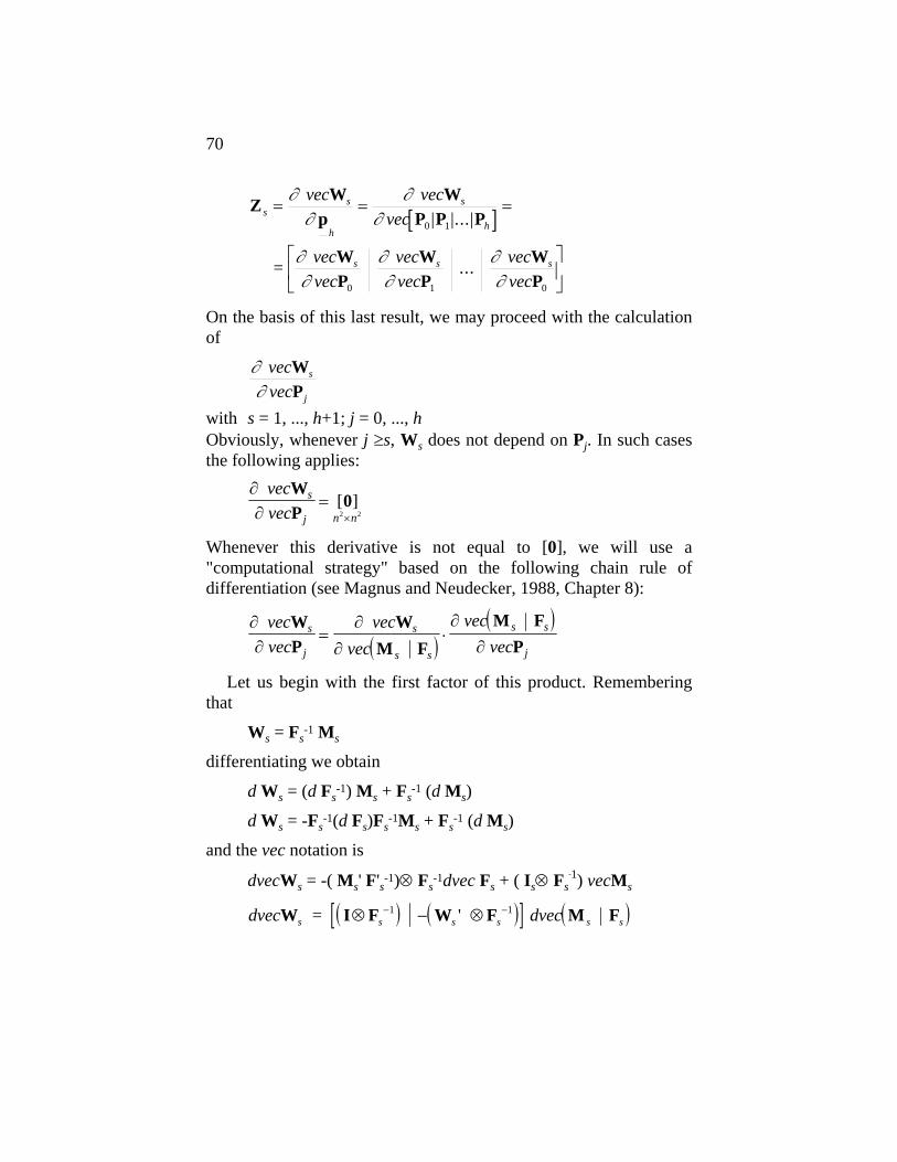
70
[ ]
Z Wp
WP P P
WP
WP
WP
ss
h
s
h
s s s
vec vecvec
vecvec
vecvec
vecvec
= = =
⎡
⎣⎢
⎤
⎦⎥
∂∂
∂∂
∂∂
∂∂
∂∂
|
=
0 1 0
0 1|...|
...
On the basis of this last result, we may proceed with the calculation of
∂∂ vecvec
s
j
WP
with s = 1, ..., h+1; j = 0, ..., h Obviously, whenever j ≥s, Ws does not depend on Pj. In such cases the following applies:
∂∂ vecvec
s
j n n
WP
0=×
[ ]2 2
Whenever this derivative is not equal to [0], we will use a "computational strategy" based on the following chain rule of differentiation (see Magnus and Neudecker, 1988, Chapter 8):
( )( )∂
∂∂
∂
∂∂
vecvec
vecvec
vecvec
s
j
s
s s
s s
j
WP
WM F
M FP
= ⋅
Let us begin with the first factor of this product. Remembering that
Ws = Fs-1 Ms
differentiating we obtain
d Ws = (d Fs-1) Ms + Fs
-1 (d Ms)
d Ws = -Fs-1(d Fs)Fs
-1Ms + Fs-1 (d Ms)
and the vec notation is
dvecWs = -( Ms' F's-1)⊗ Fs-1dvec Fs + ( Is⊗ Fs
-1) vecMs
( ) ( )[ ] ( )dvec dvecs s s s s sW I F W F M F = ⊗ − ⊗− −1 1'

71
( ) ( ) ( )[ ]∂∂
= vec
vecs
s ss s s
WM F
I F W F⊗ − ⊗− −1 1'
Now ∂∂ vecvec
s
i
WP
must be calculated. This matrix can be
represented as being composed of two n2× n2 blocks and organised as follows
∂∂∂∂
vecvecvecvec
s
j
s
j
MPFP
⎡
⎣
⎢⎢⎢⎢
⎤
⎦
⎥⎥⎥⎥
It is easy to note that
∂∂
∂∂
vecvec vec
vecs
j ji
i
sMP P
P= ∑=
−(
0
1 Pi) = ∂
∂ vec jP vec(Pj Pj)
Let us calculate this last derivative starting from the differential d(Pj Pj) = (dPj) Pj + Pj (dPj) on the basis of property a) of the Hadamard product we can write d(Pj Pj) = 2Pj (dPj) or, in vec form: d vec(Pj Pj) = 2 vecPj (d vecPj)
On the basis of property d) we can write d vec(Pj Pj) = 2 D(Pj) (d vecPj) = 2 [(vecPj ⋅ u') I
n2 ] (d vecPj) Therefore we can conclude that
∂∂ vecvec
s
j
MP
= 2 D(Pj)
where D(Pj) is the matrix previously obtained with diagonal elements equal to those of vecPj and zero elsewhere.
The same applies to the second block
∂∂
∂∂
vecvec vec
vecs
j ji i
i
sFP P
P P= ∑=
−( '
0
1 I) = ∂
∂ vec jP vec(Pj Pj' I)
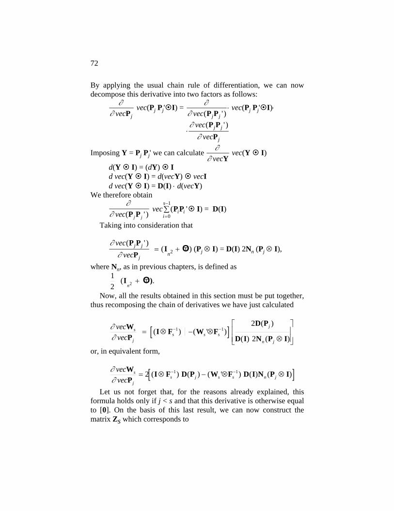
72
By applying the usual chain rule of differentiation, we can now decompose this derivative into two factors as follows:
∂∂
vec jP
vec(Pj Pj' I) = ∂∂ vec j j( ' )P P
⋅ vec(Pj Pj' I)⋅
⋅∂
∂ vec
vecj j
j
( ' )P PP
Imposing Y = Pj Pj' we can calculate ∂∂ vecY
vec(Y I)
d(Y I) = (dY) I d vec(Y I) = d(vecY) vecI
d vec(Y I) = D(I) ⋅ d(vecY) We therefore obtain
∂
∂
vec j j( ' )P P vec i i
i
s( 'P P
=
−∑
0
1 I) = D(I)
Taking into consideration that
∂
∂
vecvec
j j
jn
( ' )(
P PP
I= +2 OT ) (Pj ⊗ I) = D(I) 2Nn (Pj ⊗ I),
where Nn, as in previous chapters, is defined as
12 2 (I
n+ OT ).
Now, all the results obtained in this section must be put together, thus recomposing the chain of derivatives we have just calculated
[ ]∂∂
vecvec
s
js s s
j
n j
WP
I F W FD P
D I N P I= ⊗ − ⊗
⊗
⎡
⎣⎢⎢
⎤
⎦⎥⎥
− −( ) ( ' )( )
( ) ( )1 1
2
2
or, in equivalent form,
[ ]∂∂
2 vecvec
s
js j s s n j
WP
I F D P W F D I N P I= ⊗ − ⊗ ⊗− −( ) ( ) ( ' ) ( ) ( )1 1
Let us not forget that, for the reasons already explained, this formula holds only if j < s and that this derivative is otherwise equal to [0]. On the basis of this last result, we can now construct the matrix Zs which corresponds to

73
∂
∂∂∂
∂∂
∂∂
vec vecvec
vecvec
vecvec
s
h
s s s
h
Wp
WP
WP
WP
=⎡
⎣⎢⎤
⎦⎥0 1...
The asymptotic variance-covariance matrix of vecWs can be obtained by the formula
Σ(Ws) = Zs Σ(h) Zs' Obviously, the estimate of this matrix can be obtained by substituting the Pj matrices with their estimated counterparts $P j in all the formulae.
5.3. Finite sample and asymptotic distributions for dynamic simulations
In the first two sections of this chapter, we have seen how to construct confidence intervals around point estimates of the structural impulse response functions and the FEVD parameters, i.e. the output of the dynamic simulation of a structural VAR. We have seen that it is possible to evaluate the asymptotic distributions of the maximum likelihood estimates of those parameters, and in this way to obtain asymptotically valid confidence intervals.
The big concern in applying these techniques is then: how reliable are these measures of uncertainty when they are applied to the typical sample size of the usual macro-economic applications? In other words, are the asymptotic distributional results to be trusted when working with finite samples?
In the theoretical and applied literature, different methods have been proposed to obtain finite sample distributions of the estimated impulse response functions and FEVD parameters. The first possibility is to use bootstrapping methods (see Hall, 1994). In order to briefly explain how the bootstrap can be applied in this respect, let us write the VAR model with the same notation as used in section 1.2:
yt = Π Xt + εt , εt ~ VWN(0,Σ) where Π = [A1, A1, ..., Ap ], Xt = [yt-1', yt-2', ..., yt-p']'
or in vec form yt = (I⊗Xt) π + εt , π = vecΠ

74
and let us call $π and $Σ the estimates of π and Σ, and $ε t (t = 1, 2, ..., T) the associated residuals. A bootstrap algorithm to evaluate confidence intervals for structural impulse responses and FEVD parameters works as follows: the residuals are reshuffled N times to generate as many artificial sets of data, say Y(i), i =1, 2, ..., N, using $π as parameters of the data generation process. Then, for each
bootstrapped data set Y(i), bootstrapped estimates of the VAR
parameters are obtained, say $π( )i and $ ( )Σ i . These estimates are then used to obtain estimates of the structural impulse response functions and FEVD parameters. Storing these results for N iterations of the bootstrap algorithm yields the empirical distributions which can be used to construct the required confidence intervals 4.
Another possibility is to consider the problem under a Bayesian point of view, and to work with Monte Carlo integration (see Kloek and van Dijk, 1978). In order to give the intuition of how Monte Carlo integration can be used to obtain confidence intervals based on finite sample posterior distributions, let us consider the just-identified structural VAR case5. We indicate the prior distribution for Σ and π as p(π, Σ), and by Bayes theorem we obtain the posterior probability density function:
p(π, Σ| data) ∝ p(π, Σ) p(data |π, Σ) where the second factor is the likelihood of the model. Monte Carlo integration works as follows: generate N draws from
the posterior distribution, π(i) and Σ(i), i = 1, 2, ..., N, then map each of these draws into draws on structural impulse response functions and FEVD parameters. Storing these draws, it is possible to estimate
4 On the problems encountered when applying bootstrap methods in time series contexts, it is possible to see Li and Maddala (1996). Killian (1995) proposes a modification to the conceptually simple procedure just described, claiming to improve its properties. Anyway, Sims and Zha (1995) present results which strongly favour the use of Monte Carlo integration techniques with respect to the bootstrap. 5 Dealing with an over-identified models is less computationally straightforward than dealing with a just-identified one. Sims and Zha (1995) focuses on this problem.
75
the quantiles of the posterior distribution of the parameters of interest, which can be used to construct the required quantiles.
In the computer package RATS (Doan, 1992), a Monte Carlo integration procedure is available to construct confidence intervals for impulse responses, based on the specification of a uninformative prior of the kind:
p(π, Σ) ∝ |Σ|-(n+1)/2 Assuming Gaussian VWN errors, the resulting joint posterior
distribution for π and Σ is Normal-Inverse Whishart posterior distribution, (see Zellner, 1971) which can be easily simulated, in this way obtaining the required posterior distributions.
In order to compare asymptotic and finite sample confidence bounds for dynamic simulation parameters, we present some results contained in Amisano (1996). In that study, by using a weakly informative prior specified as to take into consideration the long-run properties of the data being analysed6, the posterior distribution of the structural impulse response functions of a just-identified model are obtained and compared to the asymptotically valid ones.
The model being studied is a tri-variate VAR system for the vector series yt = [LY, LI, LC]'t , where LY is the log of real output, LI is the log of real investment, and LC is the log of real consumption, for the US. The quarterly data7 run from 1951:1 to 1988:4. The structuralisation being used is given by the Cholesky factorisation of the variance-covariance matrix Σ corresponding to the ordering of variables: LY, LI, LC. This is clearly an exactly identified model.
In figure 5.1, we have plotted the response of the variable LC corresponding to the orthogonalised impulse in the LY equation. We report the median values8 of the posterior distributions of the
6 See Amisano (1995) for details. The prior distribution being implemented reflects the fact that the series under study are cointegrated. See chapter 6 of this book for the concept of cointegration 7 This is the data set studied in King, Plosser, Stock and Watson (1991). 8 We report the (estimated) posterior median and not the estimated mean because the Monte Carlo estimate of the latter does not necessarily comply with the requirement that the rank of C(1) be reduced in the presence of cointegration, whereas the Monte Carlo estimate of the former does. See section 6.3 for the
76
responses at different horizons, with the corresponding quantiles corresponding to the 90% confidence intervals. For the sake of comparison we also plotted the maximum likelihood estimates and the corresponding 90% asymptotic confidence intervals. In order to provide further evidence, in figure 5.2 we present the Monte Carlo estimate of the finite sample posterior distribution of one of the above mentioned impulse responses (the response at lag 5), compared to its asymptotic counterpart.
It is immediately obvious that, while the Bayesian and asymptotic ML point estimates roughly coincide, the uncertainty around the estimates is in the Bayesian case substantially higher, as implied by larger confidence sets. Moreover, the finite sample posterior distributions of the impulse response functions are interestingly skewed, even with a sample size of 152 observations. This feature is in sharp constrast with the asymptotic distributions which are based on asymptotic normality. In synthesis, this application seems to suggest some caution in applying asymptotic results, especially when working with small sample sizes.
concept of cointegration and the properties of the impulse response functions in the case of cointegration.

77
Figure 5.1: response of LC to an orthogonal shock on LY, size=90%.
Solid lines: finite sample posterior bounds and median value. Dashed lines: asymptotic bounds and maximum likelihood estimate.
Figure 5.2: response of LC to an orthogonal shock on LY after 5 periods. Solid line: finite sample posterior distribution. Dashed line:
asymptotic distribution

78
Chapter 6. Long run a priori information. Deterministic components. Cointegration
In the present chapter we discuss some issues connected to Structural VAR analysis leading to substantial deviations from the analytical apparatus described in the first five chapters of this book. We have in fact so far focused on zero mean stationary series and on the availability of exact linear constraints in order to obtain an identified structure. We remove all these hypotheses in this chapter. Section 6.1 deals with the problems induced by constraints on the long-run considerations. Section 6.2 describes the role of non-zero deterministic components in the VAR and VMA representations. Section 6.3 is devoted to the problems encountered in the analysis of the interactions between non-stationary series, in the light of the concept of cointegration, which is discussed from the viewpoint of its contrast with the concept of "spurious regression". The main representations of cointegrated systems are briefly described in section 6.3.1, in order to understand fully the different properties of a cointegrating system. Section 6.3.2 deals with the main estimation techniques available to estimate cointegrating relationships, with particular attention being devoted to the maximum likelihood analysis put forward by S. Johansen, since this is the only approach capable of delivering a testing procedure in order to make inference on the number of long-run relationships. Section 6.3.3 is devoted to the issue of the interpretation of the estimated cointegrating relationships, discussing the relevant identification conditions and the possibility of testing the validity of the over-identifying constraints. Section 6.3.4 reviews the available asymptotic results which are the basis of Structural VAR analysis as applied on cointegrated systems, and section 6.3.5 discusses the corresponding finite sample distributional results obtained via analytical and simulation studies.
6.1. Long run a priori information

79
In practical applications of Structural VAR modelling, the most interesting theoretical constraints on the parameter space of the matrices K, C, A and B, probably come from long-run considerations (see for example Blanchard and Quah (1989) for a very simple model of the C-class).
For the K-model, remembering that A(L) yt = εt K εt = et
a class of typical long-run considerations could be inserted looking at the "structural" matrix of total multipliers of the observable variables (yt ).
Calling A(1) = I - A1 - ... - Ap
the matrix of the "un-structured" total multipliers of the elements of yt and calling
A*(1) = K A(1) the matrix of "structured" total multipliers of the same variables, identification may be achieved by imposing particular constant values on certain elements of the structured A*(1) matrix. For example, for n = 2, we might consider
K A(1) = ** *
0⎡
⎣⎢⎤
⎦⎥ = A*(1)
where * inside matrices denotes a non-constrained value. Thus, in order to achieve identification we have introduced the
theoretical consideration that the total multiplier of the first variable y1t with respect to movements of the second variable y2t must be zero. This a-priori consideration algebraically implies that the inner product of the first row of the K matrix multiplied by the second column of the A(1) matrix is zero.
In the general case for n > 2 this constraint together with other constraints can always be represented with the usual formula:
R vecK = d remembering that a row (or some rows, in the case of more than one long-run constraint) of the R matrix contains elements of the A(1) matrix and some zeroes.
But in our context this type of constraints typically introduces a number of cross (bilinear) restrictions between the parameters of the

80
Π matrix (introduced in section 1.2, and collecting all the autoregressive parameters) and the parameters of the K matrix. Given these cross (bilinear) restrictions, the asymptotic information matrix:
IK
vecvec
Π⎡
⎣⎢⎤
⎦⎥
can no longer be assumed to be conveniently block-diagonal. Therefore the two-stage logic so frequently used so far for identification and estimation purposes looses its correct asymptotic statistical justification.
If we still try to use this two-stage set-up, we must remember that some elements of the R matrix must be considered as random variables (being the outcome of an estimation process), instead of being considered as constant and non stochastic. Thus, instead of using
R vecK = d in a two-stage set-up, we must work with an inexact system of constraints
$R K d = vec which will hold exactly in the limit, provided that the elements of the $R matrix are consistent estimates of the corresponding "true" elements:
plimT→∞
$R R =
Obviously, the same holds if we try to insert long-run constraints for the C-model, denoting1
C(1) = I + C1 + C2 + ... the matrix of total multipliers of "unstructured" shocks εt , and
C*(1) = C(1) C the matrix of "structured" multipliers of the structural shocks et .
Great complications arise in our set-up if we consider unstructured VAR modelling as the natural starting point for Structural VAR analysis, in this way retaining the two-stage logic.
1 If the usual stationarity condition C(1)=A(1)-1 holds.

81
The difficulties connected with the treatment of this problem are clearly depicted in Pagan (1986), a paper devoted to the properties of two-stage estimators.
As Pagan suggests, the theory of quasi-maximum likelihood estimation (White 1982) seems to be a natural tool in order to correctly analyse the problem 2. Looking at White's (1982) A1-A6 list of assumptions, on the basis of his theorem 3.1, one can immediately see that for the K-model, also in the presence of misspecification, the conditions for identification of Theorem 1 in Rothenberg (1971) are the same.
On the basis of Theorem 1 in Pagan (1986), assuming the strong consistency of our estimator of vecΠ:
vec veca s
$. .
Π Π → it can be shown that our estimator of vecK, locally identified for the K-model, retains its consistency under the kind of misspecification presented here.
In our framework, major complications arise in a quasi-maximum likelihood context for the identification and estimation of the C and AB-models. All the results in our set-up heavily draw on the so-called information matrix equivalence (see White, 1982, p. 7):
IT kE E( ) ,θ
θ θ θ θθ= −
⎡
⎣⎢
⎤
⎦⎥ = ⋅⎡
⎣⎢⎤⎦⎥ ×
∂∂ ∂
∂∂
∂∂
'
'
with 2
( )
L L L1
In the presence of misspecification, however, such equivalence breaks down and can be asymptotically restated only in the case of asymptotic negligibility of misspecifications 3.
In the light of these problems, we will proceed with the two stage logic- even if the R matrix naturally contains some (strongly
2 White (1983) shows why our two-stage set-up can be treated as his two-stage quasi-maximum likelihood estimation logic (see pp. 2.16 and 2.17), and why two-stage quasi-maximum likelihood estimation can be subsumed in the study of quasi-maximum likelihood estimation (pp. 3-11 and ff.). 3 Other complications arise when trying to find correct formulae for the calculation of impulse response functions in order to take into account the presence of a non-zero asymptotic covariance matrix between vec $Π and vec ~K .

82
consistent) estimated elements-as if the $R matrix were a "true" matrix instead of a matrix with some estimated parameters 4 .
In doing so, a warning should be introduced. Starting from the assumption that the estimator of vecΠ is strongly consistent, and that the long-run restrictions are "true", one can heuristically show that the previously described estimators of the K, C, A and B matrices are consistent. Nevertheless, the associated asymptotic variance-covariance matrices surely risk to be "poor" substitutes to correctly calculated asymptotic variance-covariance matrices which would take into proper account the inexact nature of the a-priori constraints for the K model,
$R K d vec = or similar constraints for the C and AB models.
6.2. Deterministic components Looking at the hypotheses introduced in Chapter 1,
A(L) yt = εt yt = C(L) εt
we have so far implicitly assumed that the yt vector has zero mean E (yt ) = 0
This assumption was made for exposition convenience: the analysis developed so far would remain valid with only minor modifications if we assumed that the vector of stochastic variables behave in a strictly stationary fashion around a vector of deterministic components
yt = dt + C(L) εt where dt may contain (for example) polynomial trends, seasonal dummies and dummies for outliers.
A common practice is to remove these components series by series on a univariate basis, estimating the associated parameters by OLS methods, and then estimate the VAR representation for the resulting series. In view of the results put forward by Nelson and Kang (1981) and taking into account that using these new tools in
4The natural inefficiency of the estimates vec $Π of the first stage and a consequent incorrect use of the Cramer-Rao lower bound must be taken into consideration.

83
order to find theoretically sound interpretations of cyclical movements of macroeconomic aggregates is one of the main goals of Structural VAR Analysis, it is clear that the we should not run the risk of introducing spurious periodicities.
In order to prevent the occurrence of spurious periodicities, the parameters of the deterministic components should be estimated together with the autoregressive parameters in the VAR set-up.
Assuming that the C(L) matrix of the Wold-like representation can be inverted giving as a result a finite p-order polynomial autoregressive matrix A(L), from
yt = dt + C(L) εt we can arrive at
A(L) yt = dt * + εt
with dt
* =A(L) dt For example, in the case of a vector of deterministic linear trends:
dt = ν0 + ν1 t we would have
dt * =A(L) dt = μ0 + μ1 t .
The vector autoregression with deterministic components can be written in extended explicit form as
yt = A1 yt-1 + ... + Ap yt-p + [ ]μ μ0 1
1
t⎡
⎣⎢⎤
⎦⎥ + εt
In compact form we can write yt = Π xt + εt
where xt = [yt-1', yt-2', ..., yt-p'| 1, t ] ' and the Π matrix can be thought of as composed of two distinct parts
Π = [Π1 | Π2 ], where
Π1 = [A1 | A2 | ... | Ap ], Π2 = [μ0 | μ1]
and then proceed to the estimation in the usual way following the notation introduced in Chapter 1:
$ ( )Π = −Y X' X X' 1
$ $ $ 'Σ =1T
V V

84
where $ $V X Y - = Π
Denoting as DT the matrix
1
1
13
T
T
T
np
np
np
I 0 0
0 I 0
0 0 I
[ ] [ ]
[ ] [ ]
[ ] [ ]
⎡
⎣
⎢⎢⎢⎢⎢⎢
⎤
⎦
⎥⎥⎥⎥⎥⎥
the following relationship holds: plim DT X X' DT = Q*
where Q* is a positive definite matrix. Rescaled by the DT matrix, the asymptotic distribution of the
VAR parameters is given by
( )( ) ( )D I 0 QT
dvec vec N− ⊗ − → ⊗1 $ [ ],Π Π Σ *-1
noting that
[ ]Π Π Π Π1 1 2=⎡
⎣⎢⎤
⎦⎥=
⎡
⎣⎢⎤
⎦⎥
I0
I0
np np
[ ] [ ]
and calling
JI0
=⎡
⎣⎢⎤
⎦⎥ np
[ ]
using the properties of the vec operator ( ) ( )vec vec vecΠ Π Π1 = J J I= ⊗'
from which
( )( )( )
( )( )( )( )J I D I
0 J I Q J I
' $
[ ], '
⊗ ⊗ −
→ ⊗ ⊗ ⊗
−T
d
vec vec
N
11 1Π Π
Σ
*-1
or more compactly
( )( )( ) ( )( )J I D I 0 J Q J' $ [ ], '⊗ ⊗ − → ⊗−T
dvec vec N1
1 1Π Π Σ *-1
Noting that ( )( )J I D I I'⊗ ⊗ =−
T npT1 we can get the following asymptotic distribution

85
( ) ( )( )T vec vec Nd
$ [ ], 'Π Π Σ1 1− → ⊗ *-10 J Q J
whose variance-covariance matrix is consistently estimated as: ( )[ ]T ⋅ ⊗−J X X' J' $1 Σ
Looking at the results of Chapter 5, we must insert our Π1 matrix with its associated asymptotic variance-covariance matrix instead of the Π matrix in those formulae. Obviously, the impulse response functions must be seen as impulse responses around a deterministic trend. For each series the deterministic trend around which the impulse response functions fluctuate (ν0i + ν1i t , i = 1, 2, ..., n ) can obviously be estimated by OLS methods, one series at a time, in a consistent way if the series are truly stationary around a trend.
Similar reasoning and formulae must be used in the presence of other types of deterministic components, such as seasonal dummies, dummies for outliers and intercept regime changes, obviously with a connected reasoning in the interpretation of impulse response functions.
6.3. Cointegration
Until this point, in this book we have assumed that the series being studied are stationary. In fact, it is very common to deal with series whose properties are clearly at odds with the assumption of stationarity. This is especially true for macroeconomic aggregates, so often the object of Structural VAR analysis.
In the early stage of VAR and Structural VAR analysis, it was common practice to difference the series under study as many times as required to render the differencing series stationary. Thus, non-stationarity was regarded as a nuisance, i.e. as something to be eliminated at the outset, prior to the analysis.
The last two decades have witnessed the development of univariate and multivariate inferential techniques in order to deal with non-stationary data, and in particular to deal with integrated and cointegrated series. These techniques are now part of the standard toolkit of the applied econometrician and are exhaustively surveyed in some recent advanced textbooks, such as Banerjee et al. (1993), Hamilton (1994) and Johansen (1995b).
86
The concept of cointegration is particularly important in VAR and Structural VAR analysis, since it is intimately connected to the existence and relevance of long-run equilibrium relationships among the non-stationary variables being studied. Moreover, as it will soon become apparent, cointegrated time series admit a VAR representation which can become the starting point for the specification of a structural VAR model.
The aim of this section is to briefly present the inferential techniques which are necessary to analyse cointegrated vector series, and to see how Structural VARs can be estimated and simulated when the series being analysed are cointegrated.
The issue of the interpretation of results of regressions among non-stationary variables goes back to the discussion of "nonsense regression" by Yule (1926), and the famous contribution by Granger and Newbold (1974), who refer instead to "spurious regression". The notion of spurious regression relates to a regression among non stationary variables, when good measures of fit may be found even in the absence of any direct links among the variables. This was shown with Monte Carlo simulations by Granger and Newbold (1974), and proved analytically by Phillips (1986). A very simple example of spurious regression can be provided by considering two unrelated univariate random walk processes:
Δy1t = ε1t, Δy2t = ε2t , with E (εit εjs) = 0, ### i ###j, s ###t (6.1) Both y1t and y2t are simple example of I(1) series, i.e. of series which need to be differenced once to become stationary.
The regression: y1t = β0 + β1 y2t +et
would yield an R2 index asymptotically different from zero and all the tests on the parameters (the t -tests on β0, β1 and the joint F- tests) would have diverging limiting distributions with asymptotic size equal to one. This circumstance would clearly lead to wrong inferential conclusions being drawn on the basis of any sample, no matter how large. Hence the suggestion of Granger and Newbold was to difference all variables prior to the analysis in order to eliminate the occurrence of the problem just described. Of course, this would preclude the possibility of obtaining any information on the long run relationships among the non stationary variables being analysed.

87
Long run relationships themselves are particularly interesting because they immediately relate to the notion of equilibrium links among sets of economic variables. By equilibrium is meant a state from which there is no endogenous tendency to deviate. The concept of cointegration was formalised by Granger (1981) and Engle and Granger (1987), and refers to a statistical feature of non stationary series which easily lends itself to meaningful interpretations in terms of the existence of such equilibrium relationships.
In its simplest formulation, the definition of cointegration is as follows: given yt, a (n###1) vector of I (d ) variables (i.e. series which need to be differenced d times to become stationary), they are said to be cointegrated with orders (d, b) and with rank r < n if there exist a full rank (n###r) β matrix such that zt = β'yt is I(d-b). This means that there exist r linear combinations of the elements of yt which generate variables with a lower order of integration.
The case most intensely studied in the literature is when d=b=1, i.e. when yt is I(1) and the zt variables are stationary 5. In this circumstance, it is immediate to consider the columns of β as the weights of different equilibrium relationships, and the elements of zt as the disequilibrium errors. Equilibrium relationships are relevant only if disequilibrium errors are stationary, i.e. if they are mean-reverting or, in other words, shocks that make variables deviate from their equilibrium relationships are not persistent.
To give a very simple example of this, consider two I(1) variables, x1t and x2t, and imagine that there exists a linear long run equilibrium relationship between them of the kind:
x1* = β2 x2
*. If the equilibrium relationship is relevant in determining the joint
behaviour of x1t and x2t, the disequilibrium errors should be stationary, i.e. the series
zt = β'xt = [1, -β2][x1t, x2t]' should be stationary. This would imply x1t and x2t being cointegrated with rank equal to one. On the other hand, a regression among I(1) variables in the absence of equilibrium relationships would be associated with non-stationary disturbances. This circumstance is
5 In the literature the case of cointegration among I(2) variables has also been considered. See for instance chapter 9 in Johansen (1995a).

88
then the hallmark of spurious regressions. In fact, taking for example the DGP (6.1), it is immediate to realise that:
et jj
t
jj
t= ∑ − − ∑
= =ε β β ε1
10 1 2
1
which is clearly a non stationary process.
6.3.1. Representation and identification issues In this section we will review the main representation results
concerning cointegrated I(1) variables, directly drawing from the Granger representation theorem, as stated in Engle and Granger (1987). Let us consider a n-dimensional pth order VAR process of the kind:
A(L) yt = μ0+εt, A(L) = In - A1L- A2L2-...-ApLp, εt ~ VWN(0,Σ) (6.2)
In this model the deterministic part has been kept deliberately simple for exposition purposes. Below, we will treat the issue of different, more fully articulated, deterministic components.
Suppose that the following conditions are fulfilled: (i) |A(L)| = 0 has either unit roots or roots greater than one in modulus. This condition ensures that the non stationarity of the data can be removed by differencing. The matrix autoregressive polynomial has nk roots; some of them are unity and the remaining ones are stationary. (ii) The matrix A(1) has rank equal to r <n: This means that it can be written as the product of two full rank (n###r) matrices α and β:
A(1) = -α β' This condition reflects the presence of r cointegration relations. It
ensures that the number of unit roots in the system is equal to s =n-r. (iii) The (s###s) matrix α Ψβ⊥ ⊥' has full rank s, where α###'α = β
###'β = 0 and Ψ = −⎡⎣⎢
⎤⎦⎥ =
∂∂
A( )zz z 1
, the mean-lag matrix of the VAR
representation. This condition rules out the occurrence that some of the elements of yt could be I(2) processes.
Under these conditions, the following results can be proved (see for example Banerjee et al., 1993, and Johansen 1995a): 1) Δyt and zt=β'yt are I(0) processes, meaning that they are stationary prior to any differencing.

89
2) The expected values of these stationary processes are respectively:
E(Δyt) = β###(α###'ψ β###)-1 α###'μ0, and E(β'yt) = -(α'α)-1 α'μ0 + (α'α)-1(α'ψ β###) (α###'ψ β###)-1α
###'μ0 3) The VAR system can be cast in an isomorphic error correction form (ECM):
Γ(L) Δyt = μ+αβ'yt-1+εt (6.3)
Γ(L) = Ip - Γ1L- Γ2L2-...-Γp-1Lp-1, Γ i jj i
p= − ∑
= +A
1
Notice that the relationship between VAR and ECM parameters can be easily cast in matrix form: Π = [A1, A2, ..., Ap] = W Γ + J (6.4) where
[ ] [ ] [ ][ ] [ ]
[ ] [ ] [ ][ ] [ ]
W
I 0 0 0I I 0 0
0 0 I 00 0 I I
=
−−
−−
⎡
⎣
⎢⎢⎢⎢⎢⎢
⎤
⎦
⎥⎥⎥⎥⎥⎥
n
n n
n
n n
...
...... ... ... ... ...
...
...
, J = [In , [0], ..., [0]] ,
Γ = [αβ', Γ1, ..., Γp-1 ] This matrix relationship is very useful to obtain the asymptotic distributions of the estimated VAR parameters, impulse responses and FEVD functions in the case of cointegrated series. See section 6.3.4 for the details. 4) There exists a moving average representation:
Δyt = C(L) (μ0+εt) (6.1) where:
C(1) = β###(α###'ψ β###)-1 α###' 5) It is possible to obtain a multivariate Beveridge-Nelson (Beveridge and Nelson, 1981) decomposition:
yt = y0 + Gξt + τ t + C*(L) εt G = β###(α###' ψ β###)-1, ξ α ε τ μt j
j
t= =∑⊥
=' , (1)C 0
1,
ΔC*(L) = C(L)-C(1) Some brief comments on these results seem necessary in order to
fully understand their implications. First of all, result 1) establishes

90
that the processes Δyt and β'yt are stationary while yt is not, and result 2) gives the analytical expression of the unconditional expected values of these two stationary vector processes. Result 3) allows one to write the VAR representation in an equivalent form which is particularly useful for estimation purposes. This representation is nevertheless affected by lack of identification. In fact, by choosing any invertible (r###r) matrix Q, it is possible to write:
Γ(L) Δyt = μ+α*β*' yt-1+εt where α*= αQ-1 and β*= βQ'. In order to identify α and β, it is necessary to choose a normalisation, i.e. a unique choice of the matrix Q. A widely used normalisation consists in conceptually choosing Q = β1
-1' where β1 is the upper (r###r) block of β. In this way the normalised β* matrix is β*= [Ir | β2
*']', where β2* = β2β1
-1. The result of this normalisation is sometimes referred to as Phillips' triangular representation, after Phillips (1991). On the significance of this identification problem, we will return in section 6.3.3.
Result 4) gives the impulse response function of a cointegrated system. Notice that the long run impulse response coefficients are given by the matrix C(1) which has reduced rank equal to s. Moreover, on the basis of (6.3), it is easy to see that β'C(1) = 0; therefore, the effects of shocks on zt die away as time elapses. Result 5) is particularly important in order to understand the statistical properties of the cointegrated system. Notice that the system is driven by a s-dimensional random walk process ξt. The elements of this process are the "common stochastic trends" (Stock and Watson, 1988) determining the non-stationary behaviour of yt. Choosing A = (β, τ, γ) as a basis of Rn, with γ orthogonal to β and τ, it is easy to see that along the directions of the subspace spanned by the columns of γ the process yt behaves as a s-1-dimensional driftless random walk, whereas along the directions given by the columns of β yt is a stationary process without any deterministic trend.
In the description of the properties of a cointegrated system, we have chosen to start from model (6.2), which is clearly suitable for linearly trending variables. Clearly, different alternative specifications for the deterministic part are possible, accounting for different deterministic properties of the series being modelled.

91
Following Johansen and Juselius (1990), it is possible to start from a cointegrated VAR model with a linear trend:
A(L) yt = μ0+μ1 t + εt, A(L) = Ip - A1L- A2L2-...-ApLp, εt~VWN (0,Σ) In this case, the moving average representation is: Δyt = C(L) (μ0+μ1 t + εt)
and the Beveridge-Nelson representation is: yt = y0 + Gξt + τ0 t +τ1 t2 + C*(L) εt G=β###(α###'ψβ###)-1, ΔC*(L) = C(L)-C(1)
ξ α ε τ μ μ μ
τ μ
t jj
t= =∑ + +
=
⊥=
' *, / ) ,
/
(1)( (1)
(1)
0 01
1 1
1 1
2
2
C C
C
Given that: μi = αβi + α###γi, i=0, 1 βi = (α'α)-1α'μi, γi = (α###'α###)-1α###'μi
five different cases can be distinguished: 1) μ0=μ1= 0. 2) μ0 = αβ0, μ1= 0. In this case, the constant enters the system only via the error correction term. In this case, in fact, expression (6.3) can be re-written as:
Γ(L) Δyt = α β*' yt-1* + εt, β*' = [β',β0], yt-1
* = [yt-1', 1]' 3) μ0 = αβ0+ α###γ0, μ1= 0. In this model, the parameter vector on the constant is not constrained to lie in the column space of α. In this case μ0 generates a linear trend for yt, whereas zt has no linear trend. 4) μ0 = αβ0+ α###γ0, μ1= αγ1. In this case yt has a linear trend, and so does zt. The coefficient vector μ1 lies in the column space of α, and therefore the ECM representation becomes:
Γ(L) Δyt = μ0+α β* 'yt-1* + εt, β*' = [β',β1], yt-1
* = [yt-1', t ]' 5) μ0 = αβ0+ α###γ0, μ1= αβ1+ α###γ1. With this specification, yt has a quadratic trend, whereas zt has a linear trend.
To summarise, with the use of different specifications of the deterministic part of the model, it is possible to model the particular deterministic behaviour of the series under study. It is necessary to keep in mind the presence of unit roots in the autoregressive representation. This circumstance, as in the univariate case, induces μ0 to generate a linear trend term and μ1 to generate a quadratic

92
trend term. Moreover, the reduced rank nature of the matrices A(1) and C(1) causes the leading term of the deterministic trend to have different implications, depending on whether or not the associated coefficient belongs to the space spanned by the columns of α. This fact is shown to have important consequences on the inferential procedures for testing for the cointegrating rank, r.
6.3.2. Estimation issues
When interest lies in the analysis of the long run properties of potentially cointegrated vector processes, it is first necessary to assess the number of cointegrating relationships present in the system; having done this, the weights of these relationships need to be estimated.
For expositional purposes, let us assume that we have a (n###1) vector yt of I(1) series, and that the cointegration rank is known and for simplicity equal to one; inference therefore focusses on the estimation of the coefficients of the (n###1) cointegrating vector β. In this respect, Engle and Granger (1987) suggest the use of a static OLS regression involving all the I(1) variables supposedly cointegrated, i.e. the (n###1) vector yt =[y1t, y2t']':
y zt t t= +β ' y2 The well known result by Stock (1987) ensures that the OLS
estimates are "super-consistent", in that they converge to the true parameter values at a rate T -1, instead of the rate T -1/2 as it happens in regressions involving stationary variables. In order to see this, assume that zt is stationary, and that y2t is generated according to:
Δy2t = ht where ht is a stationary vector process. Define et = [zt, ht']', and:
( )
2 0 1
1 10 1 1
0 0 0 11
21
π
f e e
e e e e
ee ( ) lim ' ' ,
' , lim '
=⎛⎝⎜
⎞⎠⎟⎛⎝⎜
⎞⎠⎟
⎡
⎣⎢
⎤
⎦⎥ = = + +
= =⎡
⎣⎢
⎤
⎦⎥
→∞
−
= =
→∞
−
==
∑ ∑
∑∑
T tt
T
ss
T
T ts
T
st
T
T E
E T E
Λ Ω Ω Ω
Ω Ω
where fee(0) is the spectral density function of et calculated at frequency ω = 0. Notice that the error term in the cointegrating regression and in the DGP for y2t are both autocorrelated and cross correlated. By exploiting the usual invariance principle and the

93
continuous mapping theorem (see Phillips and Durlauf, 1986), it is possible to show that:
T T T z
u u du u dB
t tt
T
t tt
T
d
( $ ) '
( ) ( )' ( )
β β− = ∑⎛⎝⎜
⎞⎠⎟ ∑⎛
⎝⎜⎞⎠⎟
→ ∫⎛⎝⎜
⎞⎠⎟ ∫ +⎛
⎝⎜⎞⎠⎟
−
=
−−
=
−
22 2
1
11
21
20
1
2
1
20
1
1 12
y y y
B B B Λ
where B(u) indicates a n- dimensional vector Brownian motion process6 with covariance matrix equal to Λ22. This result ensures convergence at a rate T of the OLS estimator.
The well-known problem of this estimation procedure is that simulation studies (see Banerjee et al., 1986) have shown that the finite distributions of the OLS estimates have substantial bias, persisting even in sample sizes of 100 or over.
For this reason, Phillips and Hansen (1990) propose to subject the OLS estimates to non-parametric corrections in order to mitigate the extent of the finite sample bias. Their estimator is termed Fully Modified (FM) OLS estimation and is obtained as follows:
[ ]
$ ' $ ,
$ $ , $ $$ $ , '
*
*
β
λλ
FM t tt
T
t tt
T
FM
t t t FM jj
T y T
y y E
= ∑⎛⎝⎜
⎞⎠⎟ ∑ −⎛
⎝⎜⎞⎠⎟
= − =−
⎡
⎣⎢
⎤
⎦⎥ = ∑
=
−−
=
−−
=
∞
y y y
y h e
2 21
11
2 11
1 1 12 221
2221
210
0
1
Γ
Λ Δ Γ ΨΛ
Ψ
where the ^ symbol over a variable denotes a consistent estimator of the corresponding theoretical magnitude. These estimates are obtained non-parametrically via usual kernel methods (see Newey and West, 1987, Andrews, 1991, Andrews and Monahan, 1992) starting from the residuals of the OLS estimate.
The effectiveness of these non parametric corrections is explained from two different viewpoints. First of all, using y1t
* instead of y1t is intended to reduce the effect of the long-run simultaneity, and the use of the correction −T FM $Γ serves to reduce the effect of the "second order" bias, i.e. the bias induced by the
6 For a very clear exposition of the properties of scalar and vector Brownian motion processes, and on the invariance principle and the continuous mapping theorem, it is possible to see Hamilton (1994, chapter 17).

94
autocorrelation properties of the error term et. Under a more heuristic point of view, the non-parametric corrections allow use of the information contained in the DGP for y2t in order to estimate β. This is going to reduce the extent of the bias.
The asymptotic distribution of the FM-OLS estimator is obtained as:
T u u du u dB
B u B u u
d( $ ) ( ) ( )' ( ) ,
( ) ( ) ( )
.
.
β β
λ
− → ∫⎛⎝⎜
⎞⎠⎟ ∫
⎛⎝⎜
⎞⎠⎟
= −
−
−
B B B
B
20
1
2
1
20
1
1 2
1 2 1 12 221
2Λ
The estimation methods being surveyed so far avoid facing the important issue of how to determine the cointegrating rank. The only approach that is capable of giving this problem a sensible solution is the one developed by S. Johansen (see Johansen 1988, 1991, 1995a, 1995b, Johansen and Juselius, 1990). Johansen's approach consists of the maximum likelihood analysis of the cointegrated VAR system, where inference is carried out via maximisation of the log-likelihood function. Henceforth Johansen's procedure will be referred to as MLA (Maximum Likelihood Approach).
In order to be able to write the likelihood function is clearly necessary to specify a joint distribution for the error vector εt. Then, the most natural choice would be to consider εt as multivariate normal white noise:
p([ε1', ε2', ..., εT']') = (2π |Σ|)-T/2 exp[ − ∑ −
=
12
1
1ε Σ εt t
t
T' ]
Using the ECM parameterisation (6.3), it is then possible to obtain the log-likelihood function for a finite sample of observations on yt, t = 1, ... ,T, conditional on the first p observations ( y1-p, ..., y0):
log L (α,β,Σ, Γ1, ..., Γk-1, μ) = c -(T/2)log (|Σ|) − ∑ −
=
12
1
1ε Σ εt t
t
T'
εt = Γ(L)Δyt -μ0-αβ'yt-1 The log-likelihood maximisation strategy suggested by Johansen
is based upon consecutive concentrations of the objective function. At a first step, the log-likelihood is concentrated with respect to the parameters μ, Γ1, Γ2, ..., Γp-1, yielding: logL1(α,β,Σ) = c1 -(T/2)log(|Σ|)+

95
− ∑=
12 0 1
10 1( )( )'R R R Rt t
t
T
t t− αβ − αβ' '
where R0t and R1t are, respectively, the residuals of the OLS regressions of Δyt and yt-1 on a constant and the first p-1 lags of Δyt. From the operative point of view, remember that this first step of the procedure is defined according to the deterministic components being allowed in the model. The case discussed here corresponds to the most widely used model 3), when there is an unrestricted intercept term in the ECM representation. In other cases, one would have to define in different ways these preliminary regressions. For instance, dealing with model 2), where μ0 =αβ0, Δyt and yt-1
*=[yt-1', 1]' are regressed on the first p-1 lags of Δyt.
At the second step, the log-likelihood is concentrated with respect to α:
log L2 (β,Σ) = c2 -(T/2)log (|Σ|) +
− ∑=
12 0 1
10 1( $ )( $ )'R R R Rt t
t
T
t t− α β − α β' '
$ ' , , ,α = β (β β), S S S R R01 111
10 1' ij it jt
t
TT i j= ∑ =−
=
Next, the function is concentrated with respect to Σ: log L3 (β) = c3 -(T/2)log S S S S00 01 11
110− −β β β β( )'
Given the usual partitioned matrices results, maximising the above function with respect to β amounts to minimising the ratio:
( ) / ( )β β β β β β' ' 'S S S S S11 10 001
01 11− − (6.5) This context is very similar to the L.I.M.L. estimation approach (see for instance Davidson and Mc Kinnon, 1994, pp. 644-651). It is therefore possible to work with the normalisation β'S11β = Ir, and show that the (n###r) matrix β which minimises (6.5) is given by taking the r generalised eigenvalues of S S S10 00
101
− with respect to S11, corresponding to the r largest eigenvalues . The maximum of the log-likelihood function is therefore:
( )
( ) ( )
log ( ) / log| $ $ $ ' |
/ log| $ | / log( $ )
*L r c T
c T c T
r r r
r r ii
n
= − − =
− − = − −∑
−
=
2
2 2 1
11 10 001
01
1
β β β
Ι
'
=
S S S S
Λ λ

96
where $Λ r is a(r###r) diagonal matrix with the r largest generalised eigenvalues on its main diagonal.
It is possible to provide a different interpretation to the MLA estimator. In fact, as stressed in Johansen (1988), the estimates of β and α are related to the canonical variates between R0t and R1t (see Anderson, 1984): the ML estimate of β corresponds to the r linear combinations of yt-1 having the largest squared partial correlations with Δyt, after having corrected for the effects of the variables appearing as regressors in the preliminary regressions. This interpretation of the estimates is based on the nature of reduced rank regression of the ECM representation.
On the basis of these results, it is possible to construct a likelihood ratio test in order to test H0: cointegration rank = r against the alternative H1:cointegration rank = n:
LR(r/n) = − −∑= +
T ii r
nlog( $ )11
λ
and this test is known as the trace test. In the same way, it is possible to obtain the likelihood ratio test in order to test H0: cointegration rank = r against the alternative hypothesis H1: cointegration rank = r+1:
LR(r/r+1) = − − +T rlog( $ )1 1λ known as λ-max test.
The finite sample distributions of these statistics are completely unknown, but the asymptotic properties have been deeply analysed (see for instance chapter 11 in Johansen 1995a). For ease of exposition, let us concentrate only on the trace test. It is possible to show that the following result holds:
− −∑ → ∫ ∫⎡⎣⎢
⎤⎦⎥
∫⎧⎨⎩
⎫⎬⎭= +
−
T trace d d dii r
n dlog( $ ) ( ) ' ' ( )'11 0
1
0
1 1
0
1λ W F FF W F W (6.2)
where W denotes a standard Brownian motion process in p-r dimensions, and F is a function of W defined in different ways depending on the particular deterministic part of the model. Recalling the five different models described above: 1) When μ0 = μ1 = 0, F(u) coincides with W(u). 2) When μ0 = αβ0, and μ1 = 0, F(u) has p-r+1 dimensions and we have:

97
Fi(u) = Wi(u), i = 1, 2,..., p-r; Fi(u) = u, i = p-r+1.
3) When μ0 = αβ0+α###γ0, and μ1 = 0, we have: Fi(u) = Wi(u)-###Wi(u)du, i=1, 2,..., p-r-1, Fi(u) = u-1/2, i=p-r.
4) When μ0 = αβ0+α###γ0 and μ1 = αβ1, the F(u) process is p-r+1-dimensional, and is defined as:
Fi(u) = Wi(u)-###Wi(u)du, i=1, 2,..., p-r, Fi(u) = u-1/2, i=p-r+1.
5) Finally, when both μ0 and μ1 are unconstrained, the F(u) process has p-r dimensions and it is defined as:
Fi(u) = Wi(u)-ai-biu , i=1, 2,..., p-r-1 Fi(u) = u2-a-b u, i=p-r
where the coefficients ai, bi, a and b are obtained by regressing respectively Wi(u) and u2 on an intercept and a linear trend.
If the deterministic part of the model were different from any of the five cases described above, the asymptotic distribution results could be radically different. Everything depends on which term asymptotically dominates the deterministic behaviour of the process. For instance, the presence of an intercept-shifting dummy variable would modify the asymptotic distributions of the cointegrating rank statistics in case 3, i.e. when the leading deterministic term is the constant term, but it would not change anything in case 5, where the leading deterministic term is a linear trend.
In synthesis, dependence of the asymptotic distribution (6.5) on the deterministic part of the model renders inference somehow problematic. Exactly as happens in univariate unit root testing 7, we need to determine correctly the deterministic features of the model, in order to conduct correct inference on the stochastic features of the series under study. Hence the inferential results are somehow conditional on the choice of the deterministic component being valid.
Ironically, the restrictions associated with each of the different deterministic components described above could be tested by means of a standard asymptotically χ2distributed LR test, given the cointegrating rank, as we will see when dealing with the
7 See Hamilton (1994), chapter 17.
98
distributional properties of the estimates. The implicit circularity of the procedure is evident.
In order to cope with the problem, Johansen (1992) follows Berger and Sinclair (1984) and Pantula (1989) and specifies an approach based on testing a nested sequence of hypotheses. The main idea behind this approach is to reject an hypothesis only if the hypotheses contained in it are rejected. For instance, let us suppose that it is not clear whether to adopt model 2) or model 3) as the best description of the deterministic feature of the data. Defining Hi(r) as the rank r hypothesis in model i (=2 or 3), and ci(r) the α% quantile of the asymptotic distribution of the corresponding trace test statistic Qi(r), Johansen proposes to reject Hi(r) if the collection of test results for all the contained hypotheses belong to the set:
{Qh(k) >ch(k), ### h, k such that Hh(k) ### Hi(r)} and to accept Hi(r) if the collection of test results for all the contained hypotheses belong to the set:
{Qh(k) >ch(k), ### h, k such that Hh(k) ### Hi(r), and Qi(r) <ci(r)}
This testing procedure consists in testing a sequence of hypotheses where the hypotheses further on in the sequence contain all the preceding ones. Johansen (1992) shows that this procedure is consistent and it has asymptotic size equal to α. Of course very little is known about the finite sample properties of this testing procedure: "The inference conducted here is asymptotic and simulations show that one can easily find situations in practice where the number of observations is not sufficient to apply asymptotic results" (Johansen, 1995a, chapter 11).
6.3.3. Interpretation of the cointegrating coefficients
As stressed in the previous section, the cointegrated ECM model is affected by a lack-of-identification problem. In Johansen's maximum likelihood approach this lack-of-identification problem is solved by adopting the normalisation β'S00β=Ir. Of course, this normalisation does not necessarily have any economically meaningful interpretation.
Johansen and Juselius (1994) and Johansen (1995b) give a solution to the problem of the interpretation of the cointegration relationships by casting it into a classical identification problem.

99
The cointegration relationships β' yt = zt can be interpreted as a system of r linear equations. In order to achieve identification, it is possible to impose a set of constraints on each equation. A set of r normalisation constraints is needed in order to impose a unit coefficient on one of the variables in each equation. Leaving these trivial constraints aside, Johansen considers linear homogeneous constraints of the kind : Ri βi = 0, i=1, 2, ..., r (6.6) where βi indicates the i-th column of β and Ri is a (r###qi) full column rank matrix. The same constraints can be expressed in explicit form as follows:
βi = Hi φi, i=1, 2, ..., r, Ri Hi = 0 (6.7) Following Sargan (1988), identification of the i-th equation is
achieved when the following rank condition is fulfilled: ρ (Ri β)=r-1
meaning that the "structural" ith equation, i.e. the one obeying the constraints (6.6) cannot be generated as a linear combination of the other columns of β. The rank condition is satisfied only when the order condition qi ### r-1 is fulfilled.
Nevertheless, it is problematic to check the rank condition because it impinges upon the values of unknown parameters. For this reason, Johansen (1995b) puts forward another formulation of the rank condition which is entirely based upon the structure of all the constraints being imposed upon β. The constraints imposed on the system are such to identify the i-th equation if and only if:
[ ]{ }ρ R H H Hi j j jkk
1 2| |...| ≥
for every set jk, 1<j1<j2<...<jk ... ### r with k=1, 2, ..., r-1. If the i-th equation is identified and the rank condition is satisfied as qi=r-1, then the equation is exactly identified, and no constraint is actually being imposed on it. If, instead, the i-th equation is identified and qi>r, the equation is overidentified and qi-r+1 constraints are actually being imposed on it. In order to fully understand this concept, let us consider Phillips's triangular representation as a particular example of exact identification. The particular structure being imposed on the cointegrating relationships complies with Johansen's identification conditions, and it does not entail any constraint being imposed on the parameter space; in fact, leaving

100
aside the normalisation constraint forcing the ith variable to appear with a unit coefficient in the ith equation (i=1, 2, ..r), on each equation we have r-1 exclusion restrictions: all the equations are exactly identified and no restriction is being imposed on the parameter space. From a different viewpoint, this finding is corroborated by the fact that the triangular representation can be obtained by simple algebraic transformation of the unrestricted estimation which is obtained subject to the normalisation β' S11 β = Ir .
When over-identifying constraints are being imposed, their legitimacy can be tested by means of Wald or likelihood ratio test statistics. Using the LR testing principle requires estimation of the model subject to the restrictions. This can be achieved by means of a switching algorithm which works as follows: starting from an arbitrary initialisation, one cyclically solves the reduced rank regression algorithm for each one of the columns of β, imposing all the constraints and considering all the other columns of β as given. This is shown to converge to the maximum likelihood estimation under the hypothesis that the over-identifying constraints hold. A LR test can be easily constructed, and Johansen (1995b) shows that the resulting statistic is asymptotically χ2 distributed with as many degrees of freedom as the number of over-identifying restrictions being imposed on the parameter space.
6.3.4. Asymptotic distributions of the parameter estimates: Structural VAR analysis with cointegrated series
After having adopted a normalisation to identify the cointegration relationships parameters (for instance the triangular representation normalisation), the asymptotic distribution of the estimates can be obtained by Taylor expansion of the log-likelihood function. For the sake of brevity, we only deal with the case in which the deterministic part is equal to μ0. The asymptotic distributions applying in all the other cases can be easily obtained by appropriately modifying the Brownian motion processes involved.

101
Working with the normalisation [ ]C C C 0' $ ' , ' | ,β = β = Ι Ιr r= which corresponds to the triangular representation, theorem 12.3 of Johansen (1995a) proves the following result :
T du d
du du
u u du u
u
d
n( $ ) ( ' ) ' ( )'
' '
' ( ) ( ) ( ) , /
( ' ) ( ), '
. . .
.
β − β β γ
γ
α Σ α Σ γ = γ(γ γ)
0
1
0
1
α
0
1
0
1
0
1
α−1 −1 −
→ − ∫⎡⎣⎢
⎤⎦⎥
∫
= − ∫ ∫⎡⎣⎢
⎤⎦⎥
= − ∫⎡⎣⎢
⎤⎦⎥
= −
=
−
−
−
I C G G G V
G G G G G G G
G C W W G
V W
1 2 1 2
1
1 2
1 2 1 1 2 2 2
1
2
1 2
1 1
1 1 2
W(u) in this context indicates a vector Brownian motion with covariance matrix equal to Σ, and γ is a (n###(s-1)) matrix orthogonal to β and to the coefficient vector of the leading deterministic term in the Beveridge-Nelson representation.
This result tells us two things: 1) As in the static regression, the normalised coefficients in β are super-consistent , since they converge at a rate T-1 to their true values; 2) the asymptotic distribution of Tvec( $ )β β− is mixed-Normal, with mixing covariance matrix given by:
[ ]( ' ) ( ') ' ( ' ). .α Σ α β γ γ β−1
0
1−
−
⊗ −⎡
⎣⎢
⎤
⎦⎥ −
⎧⎨⎪
⎩⎪
⎫⎬⎪
⎭⎪∫1
1 2 1 2
1
I C G G I Cn ndu '
which can be consistently estimated as: [ ] { }T n n( $ ' $ ) ( $ ' ) ( $ ' )α Σ α β β−1 − −⊗ − −1
111I C S I C
given that we will see that $α is a consistent estimator for α. The circumstance that $β is asymptotically mixed-Normal means
that, conditionally on the estimate of the mixing covariance matrix, it is possible to use the standard distribution theory which will be asymptotically valid. Nevertheless, one has to take into account that the marginal asymptotic distribution of $β will have fatter tails than a Normal distribution.

102
When over-identifying constraints such as the ones described in expression (6.7) are imposed on the cointegrating vectors, and a unit normalisation has been imposed such that the constraints become:
βi = Hiφi+hi, sp(hi, Hi) = sp(Hi), i = 1, 2, ..., r, Ri'Hi = 0 the asymptotic distribution of T⋅vec( $β ) is still mixed-Normal, but the mixing covariance matrix is different from the one described above, and it can be consistently estimated as:
{ }{ } { }T ii j
i j iH H S H H(α Σ α−1$ $ $ ) ' ''11
1−
In the above expression the notation {Ai} i=1, 2, ..., r, indicates a block diagonal matrix with ith block equal to Ai, and {Aij}, i, j=1, 2, ..., r, means a partitioned matrix with blocks Aij.
The super-consistency property of the cointegrating vector coefficients allows one to obtain the asymptotic distributions of the estimates of the loading factors and of the parameters connected to the short run dynamics. In fact, given super-consistency of $β , β can
be asymptotically considered as known: in fact, $β has a non-degenerate limit distribution only when scaled by T , whereas asymptotic distribuitons are evaluated for the estimates of the loading factors and of the short-run dynamics parameters, which are scaled by T1/2. Writing the ECM representation (6.3) as:
[ ]
[ ]Δ Ξ Ξ~ ~ , |...| ,
' ' |...| ' '
y z
z y y y
t t t p
t t t t p
= + =
=
−
− − − +
ε α | Γ Γ
β | Δ Δ
1 1
1 1 1
(6.8)
where the ~ symbol over a variable means the residuals of a regression of that variable on the unrestricted deterministic part of the ECM model, it is clear that, were β known, all the variables appearing in (6.8) would be stationary. For this reason, standard asymptotic results apply for the parameters in Ξ:
[ ]T vec Nd
t1 2 1/ $ ( , ), var( )Ξ Ξ− → ⊗ =−0 zΩ Σ Ω
This allows the use of standard asymptotic results also on the parameters of the VAR representation, since these are linear functions of the elements of Ξ, considering β as given, given that its estimate is super-consistent.
In fact, it is easy to see that

103
Γ = Ξ B, Γ = [αβ', Γ1, ..., Γp-1 ],
[ ]
[ ]B0
0 I=
⎡
⎣⎢
⎤
⎦⎥
−
β'
(n p 1)
Therefore, since the parameters in Γ are given by a linear transformation of the matrix Ξ, given β, we have:
[ ] ( )[ ]T vec N
d
k
1 2 1
1 1
/ $ , ' ,
$ $ $ ' , $ , ... , $
Γ Γ
Γ = α β
− → ⊗
⎡⎣⎢
⎤⎦⎥
−
−
0 B B
Ω Σ
Γ Γ
and, recalling the expression (6.4):
[ ] ( )[ ]T vec Nd
1 2 1/ $ , ' 'Π Π− → ⊗−0 W B BW Ω Σ
This result is particularly important, since it can be used as a starting point for the specification, the estimation and the dynamic simulation of a Structural VAR model. In fact, when the variables being considered in the analysis are cointegrated, the ECM parameterisation is estimated via maximum likelihood, subject to the constraints given by the cointegrating rank. Also, some over-identifying constraints could be imposed on the cointegrating relationships, when they are necessary to provide them with a meaningful interpretation. At this stage, the resulting ECM estimates
are then mapped into an estimate of the VAR parameters $Π , given the linear relationship (6.4). This estimate, together with its asymptotic variance-covariance matrix and the maximum likelihood
resulting estimate of the vector error term $Σ , can be used as a starting point for Structural VAR analysis, using the analytical apparatus described in the first five chapters of this book.
As a final remark, notice that , in the case of a cointegrated VAR model, it is possible to use constraints on the matrix of structuralised loadings in order to achieve an identified Structural VAR. In fact, as an example, let us consider the K-model in the equivalent ECM form Γ*(L) yt = α* β' yt-1 + et , Γ*(L) = K Γ(L), α* = K α The α* matrix of structuralised loadings could have a zero as i-th row, j-th column element if there are reasons to believe that the j-th disequilibrium error (j-th element of zt-1 = β'yt-1 ) is not "loaded" on

104
the i-th structural equation. Keeping in mind the caveat explained in the first section of this chapter, these homogeneous restrictions can be easily accommodated with the usual formula: R vecK = d In section 9.1 we provide an example where a Structural AB model is identified using also constraints on the structuralised loading matrix.
6.3.5. Finite sample properties
In the previous section we have reviewed the asymptotic distributions of the maximum likelihood estimate of the long-run parameters in a cointegrated VAR model. These results are the basis of all the inferential procedures being widely used in the applied literature. Blind reliance on asymptotic results can be dangerous, given that in the typical macroeconomic application it is very common to work with very short sample periods. Therefore, it is extremely useful to investigate small sample properties of the ML estimates and, more generally, the properties of the test statistics being used to guide key decisions concerning the specification of the model.
From the theoretical point of view, a recent paper by P.C.B. Phillips (1994) has investigated the exact finite sample distributions of the normalised reduced rank estimates of the cointegrating parameters. The analytical results obtained by Phillips echo the analogous results concerning the exact finite sample distribution of L.I.M.L. estimates in a simultaneous equation model (Phillips, 1983), and this is not surprising given the already mentioned analogy between the ML estimate of β and the L.I.M.L. estimator.
Analysing a simple ECM model as in (6.3) but without deterministics, and working with the normalised estimates
[ ]$ | $ ' 'β = Ι φr , Phillips discovers that the leading term of the finite
sample distribution of $φ is proportional to |Ir+ $φ ' $φ |-n/2, i.e. to the kernel of a matrix-Cauchy distribution. The exact shape of the distribution is in general very complicated, but its tail behaviour is generated by the matrix-Cauchy term. This feature means that the finite sample distribution does not have finite moments of integer order. From a different viewpoint, the free parameters in the
105
normalised estimates are obtained as the ratio of two blocks of the ML estimates; as stressed in Sargan (1988) and Phillips (1983), this is enough to prevent the finite sample distribution of the resulting coefficients from having finite moments of integer order. As Phillips (1994) emphasises, the Cauchy-like tail behaviour is therefore not a consequence of the circumstance that the asymptotic distribution of $φ is mixing-normal, i.e. that in the limit the sample information is
random: in fact, Phillips' (1991) estimator based on the triangular representation does not have Cauchy-like tails. However, it is necessary to keep in mind that this estimator does not allow to conduct inference on the cointegrating rank. Some Monte Carlo simulation studies shed further light on the finite sample properties of cointegrating coefficient estimators. Cappuccio and Lubian (1995) conduct a very interesting experiment simulating a six-variate cointegrated DGP with rank equal to two and subject to over-identifying restrictions on the cointegrating parameters.
Then they estimate a ECM model subject to the over-identifying restriction for each data set and for different sample sizes. At each step also the tests of the over-identifying constraints are computed. Their results can be summarised as follows. a) The reduced rank regression ML estimates do not show significant finite sample bias, but they have huge numerical standard errors, reflecting the Cauchy-like tails of the finite sample distributions. The occurrence of outliers in the estimates becomes negligible only for sample sizes of 200. This means that the any applied macroeconomic researcher should be extremely careful in relying on the asymptotic distributions of the parameter estimates. b) Even more alarmingly, the finite sample distributions of the LR test used to check the validity of the over-identifying restrictions are very different from their asymptotic χ2 counterparts. For a sample size of 50, and high values of the time dependency of the ut process, the actual size of the testing procedure applied with a nominal size of 5% is almost 80%, clearly leading to extreme over-rejection of the null hypothesis. Only with sample sizes equal to 300, does the actual test size tend to become close to the nominal one.
These simulation results clearly signal that the finite sample properties of the MLA can be substantially different from their asymptotic counterparts. In our view, these results should suggest

106
some caution to the applied researcher who wants to use cointegration techniques. In our experience, it is not uncommon to find very strange and hard to interpret results in the rank and identification analysis, when dealing with small samples. This fact can be easily interpreted as empirical evidence of the Cauchy tail behaviour of the maximum likelihood cointegrating relationships estimates. In that respect, we can put forward the following suggestions.
As for the determination of the cointegrating rank, further (and sometimes conclusive) evidence can be gained by recursive techniques (for details see Hansen and Johansen, 1993): the cointegrated model is estimated and the relevant statistics are computed recursively adding one observation at a time. In this way it is possible to (informally) assess the robustness of full sample results. Anyway, the recursive approach is not capable of solving the problem of the poor sample properties of the MLA approach. Recently some attempts have been made in order to obtain finite sample corrections for asymptotically based unit root tests (see Nielsen, 1995); future research might produce the multivariate version of these corrections necessary to deal with the problem of rank determination. One of the two authors is currently working on a Bayesian inferential procedure, based on finite sample evidence, in order to deal with (possibly) cointegrated systems8.
As for the problem of estimating and interpreting the cointegrating relationships, the application of the FM-OLS approach described in section 6.3.2 has shown appreciable finite sample properties. This remark could suggest the use of a two-stage logic: estimate the long-run relationships by FM-OLS and then plug these estimates into the ECM model to obtain an estimate of the other parameters of the system. At this point one could then start the specification of a Structural VAR model.
8 Amisano (1996).

107
Chapter 7 Model selection in Structural VAR analysis
In this chapter we explain how to use the dominance ordering and the likelihood dominance criteria introduced by Pollack and Wales (1991) as model selection devices in Structural VAR analysis1. In section 7.1 we recall the main aspects of model selection and we connect this issue directly to the Structural VAR framework. The next two sections are devoted to explaining the above mentioned model selection criteria. 7.1. General aspects of the model selection problem
In many Structural VAR applications, the researcher faces the problem of choosing among competing identifications of the A and B matrices. Different economic theories often suggest the imposition of different sets of constraints, all equally plausible from the economic point of view. It is therefore necessary to have a criterion in order to decide which identified structure is best supported by data evidence.
Considering the model selection problem from a more general viewpoint than that of Structural VAR analysis, Harvey (1990) indicates five model features which can be used in order to assess the relative validity of competing models. These features are: 1) Parsimony: models with fewer parameters are preferred for statistical and interpretative reasons. 2) Identifiability: identified models are preferred to unidentified ones. 3) Fitting performances: this feature is usually assessed by means of statistical tests on the residuals. 4) Predictive power: models are often ranked according to their forecasting performances.
1 For detailed accounts on model selection problems, see Pesaran (1974) and McKinnon (1983).

108
5) Economic consistency: models producing results which are difficult to explain theoretically tend to be considered as less reliable.
In Structural VAR analysis, the criteria 2) and 5) are particularly important, and in applied contexts are often used to informally discriminate among competing structures of the A and B matrices. In particular, the identification conditions and the statistical test of the over-identifying constraints described in chapters 2, 3 and 4 of this book are valid instruments in order to guide model selection. In many circumstances though, it is possible that a choice should be made between two (or more) over-identified structures whose over-identifying constraints are supported by the data. In this case, a statistically based criterion would be highly appreciated in order to help the applied researcher make a sensible choice.
In this respect, two model selection criteria have been put forward by Pollack and Wales, based on the concept of "likelihood dominance", which will be explained in the remaining sections of this chapter. These criteria are based on indexes depending on the likelihood functions of the estimated models. For this reason, in Structural VAR analysis they can be applied only to contexts where some of the models being compared are over-identified, because no likelihood based criterion is available in order to discriminate among exactly identified models. Therefore, for exposition convenience, we imagine that the problem is that of deciding between two Structural VAR models, M1 and M2 , generated from the same reduced form VAR model and producing economically sensible results. Pollack and Wales (1991) propose two criteria, namely the dominance ordering (DO) and the likelihood dominance criterion (LDC), which will be exposed in the following two sections. 7.2. The dominance ordering criterion
The DO criterion is based on the comparison of two non-nested models, M1 and M2, with reference to a more general model, say Mc (the composite model) intended to embed both models. Notice that there is no need to actually estimate Mc . It is only necessary to be able to know the number of free parameters of Mc , and to estimate by maximum likelihood M1 and M2. In fact, the DO criterion is

109
based on the comparison of the maximised likelihoods of the two models, exactly as it happens for the usual likelihood ratio (LR) tests.
In order to explain how the criterion works, we imagine to have estimated also Mc, and to have the values of the maximised log-likelihoods for the three models, say L1, L2 and Lc . And We indicate with l1, l2 and lc the number of free parameters in each model. The comparison between M1 to Mc can be done by constructing a LR test. M1 is then preferred to Mc if
2 Lc - 2 L1 < Cα (lc -l1) where Cα (h) is the α % critical value of a χ2 distribution with h degrees of freedom. If we apply this criterion to M1 and M2 , we can have only the following four outcomes: 1) M1 is accepted and M2 rejected if: Cα (lc -l1) > 2 Lc - 2 L1 and Cα (lc -l2) < 2 Lc - 2 L2 2) M1 is rejected and M2 accepted if: Cα (lc -l1) < 2 Lc - 2 L1 and Cα (lc -l2) > 2 Lc - 2 L2 3) M1 and M2 are both rejected if: Cα (lc -l1) < 2 Lc - 2 L1 and Cα (lc -l2) < 2 Lc - 2 L2 4) M1 and M2 are both accepted if: Cα (lc -l1) > 2 Lc - 2 L1 and Cα (lc -l2) > 2 Lc - 2 L2
The DO criterion focuses on the outcomes 1) and 2) and aims at excluding one of the two by considering only L1 and L2 and the number of free parameters in the composite model. To this end, let us define the "adjusted likelihood value" as:
Vi = Li + Cα (lc -li)/2, i = 1, 2 Now, when V1 < V2 the maximised log-likelihood of Mc surely belongs to one of the following three intervals: (-∞, V1), (V1, V2), (V2, +∞)
When Lc < V1 we are in the situation 4) described above, i.e. when both M1 and M2 are accepted. When Lc ∈ (V1, V2) we are in case 2), i.e. M1 is rejected and M2 accepted. When Lc > V1, then both models are rejected in favour of the composite model Mc . It is important to notice that when V1 < V2 , there is no value Lc such that M2 is rejected and M1 accepted; in other words, case 1) never applies when V1 < V2.

110
Analogous considerations should be made when V1 > V2. In that case, depending on the unknown value of Lc , it cannot happen that M1 is rejected and M2 accepted against Mc .
At this point we can formulate the following proposition: DO criterion for model selection:
According to the DO criterion, M1 and M2 can be ordered as follows: 1) M1 is preferred to M2 if V1 > V2 2) M2 is preferred to M1 if V1 < V2 3) M1 is equivalent to M2 if V1 = V2 Since this decision rule is transitive, it allows any class of alternative models to be given a complete ordering, and to choose the "best" one among them (according to the criterion).
This criterion is extremely simple (if not trivial): it is extremely easy to compute L1, L2 , and to choose a test size α . A bit more problematic is the choice of Mc , given that in certain applied contexts it is not clear which is the composite model.
In this respect, let us consider model comparison in Structural VAR analysis. In this case, it would be natural to consider Mc as a just identified model and therefore to conclude that
lc = n (n+1)/2 It is worth pointing out that in certain situations the composite model corresponding to M1 and M2 is not necessarily an exactly identified one. In our view, it would be more correct to consider Mc as the model obtained by taking the logical "intersection" between M1 and M2 . In order to make a simple example, consider the case when
M1 : A1
1 0 0 0
0 1 0 0
0 1 0
0 1
=
⎡
⎣
⎢⎢⎢⎢⎢⎢
⎤
⎦
⎥⎥⎥⎥⎥⎥
*
* *
, B1
0 0 0
0 0 0
0 0 0
0 0 0
=
⎡
⎣
⎢⎢⎢⎢⎢⎢
⎤
⎦
⎥⎥⎥⎥⎥⎥
*
*
*
*

111
M2 : A2
1 0 0 0
0 1 0 0
0 0 1 0
0 0 1
=
⎡
⎣
⎢⎢⎢⎢⎢⎢
⎤
⎦
⎥⎥⎥⎥⎥⎥*
, B2
0 0 0
0 0
0 0 0
0 0
=
⎡
⎣
⎢⎢⎢⎢⎢⎢
⎤
⎦
⎥⎥⎥⎥⎥⎥
*
* *
*
* *
where * denotes a free parameter. In this case we have l1 = 7 , l2 = 7, and the logical "intersection" of the two models is
Mc : A c =
⎡
⎣
⎢⎢⎢⎢
⎤
⎦
⎥⎥⎥⎥
1 0 0 00 1 0 00 1 0
0 1*
* *
, B 2
0 0 00 00 0 00 0
=
⎡
⎣
⎢⎢⎢⎢
⎤
⎦
⎥⎥⎥⎥
** *
** *
It is easy to see that M1 and M2 are nested in Mc as particular cases, even if it is not exactly identified since it has 9 free parameters instead of 10.
On the other hand, the logical "intersection" between M1 and M2 could be an unidentified model. In fact, it is possible that the resulting Mc model has too many free parameters, or that it is anyhow unidentified and in that case the FIML estimation of Mc is not feasible. In any case, this does not prevent the application of the DO criterion, since the actual estimation of the composite model is not required.
In the case when l1 = l2 , i.e. when the two models being compared have the same number of free parameters, it is easy to see that it is not necessary to compute the two adjusted likelihood values, since
Cα (lc -l1) = Cα (lc -l2) and hence the DO comparison between the two models can be done on the basis of the two maximised log-likelihoods, and the choice of the composite model is completely immaterial. 7.3. The likelihood dominance criterion (LDC)
In the previous section we have seen that the DO criterion is influenced by the number of free parameters of Mc .The nature of this dependence is more evident if we re-write the DO rule as follows:
112
M2 is preferred to M1 (or, in other words M2 dominates M1) if and only if L1 -L2 > [Cα (lc -l1)- Cα (lc -l2)]/2 (7.1)
In the absence of any certain information about the parametric dimensionality of Mc , Pollack and Wales (1991) suggest a more general criterion than DO, in order to side-step the need to determine the precise value of lc , the number of free parameters in Mc . Pollack and Wales suggest studying the behaviour of the r.h.s. of (7.1) for different values of lc .
Calling Cα
* (lc , l1 , l2) = [Cα (lc -l1)- Cα (lc -l2)]/2 on the grounds of numerical explorations, Pollack and Wales found that when l1 > l2, Cα
* (⋅) is monotonically decreasing in lc when α is below 40%. When l1 < l2 Cα
* (⋅) is monotonically increasing in lc when α is below 40%.
Now, let us assume that l1 < l2 . Clearly, lc has then a lower bound given by
min(lc) = l2 +1 given that M1 and M2 are non-nested. As for the upper bound of lc , Pollack and Wales point out that lc cannot be larger that l1 + l2 +1. In the Structural VAR context such an upper bound can be considered as sensible, although in certain applications other upper bounds might be legitimately considered.
Anyhow, having determined min(lc) and max(lc), it is clear that Cα
*(lc , l1 , l2) has its maximum in min(lc) and its minimum in max(lc), given that it is monotonically decreasing in lc As a consequence of this, the quantity L1-L2 belongs to one of the following three intervals: (-∞, Cα
*(max(lc), l1 , l2)), (Cα
*(max(lc), l1 , l2), Cα*(min(lc), l1 , l2)),
(Cα*(min(lc), l1 , l2) , +∞)
When L1 -L2 > Cα*(min(lc), l1 , l2), then condition (7.1) holds for any
value of lc . In the same way, if L1 -L2 < Cα*(max(lc), l1 , l2), then
condition (7.1) cannot hold for any value of lc . Obviously it might be the case that for some values of lc condition (7.1) holds, whereas it does not for other values of lc . In this case the LDC is indecisive between M1 and M2 .
113
In synthesis, Pollack and Wales formulate the following proposition: 1) M1 is preferred to M2 if L1 -L2 < Cα
*(max(lc), l1 , l2)
2) M2 is preferred to M1 if L1 -L2 > Cα*(min(lc), l1 , l2)
3) No decision can be taken if Cα
*(max(lc), l1 , l2) < L1 -L2 < Cα*(min(lc), l1 , l2)
The possibility of indecisive outcomes in real applications raises the possibility that the LCD criterion might not yield a coherent and complete ordering in a class of more than two models, unlike what happens when the DO criterion is applied. In this cases, it is straightforward to reduce the indecisive region of the LDC by shrinking the size of the interval between min(lc) and max(lc). When the size of this interval becomes zero, the LDC is fully equivalent to the DO criterion. As a final remark, exactly as happens with the DO criterion, when l1 = l2 the application of the LDC amounts to comparing the maximised log-likelihoods of the two models.

114
Chapter 8 The problem of non fundamental representations
The validity of dynamic simulation results obtained from Structural VAR model has been very strongly criticised in two recent papers (Lippi and Reichlin, 1993 and 1994). The content of this criticism is closely connected to the existence and the relevance of non fundamental MA representations (see Hansen e Sargent, 1991, ch. 4). We start this chapter by describing the content of the Lippi and Reichlin criticism. Section 8.1 is devoted to explain the notion of non fundamental representation in time series models. Section 8.2 presents some examples of economic models generating non fundamental representations and section 8.3 connects the issue of the existence of non fundamental representations to Structural VAR analysis, presenting a new way to assess the relevance of these representations in particular applications. An applied example of this procedure is contained in section 8.4. 8.1. Non fundamental representations in time series models
In order to fully understand the problem related to the existence and relevance of non-fundamental representations (henceforth NFRs), let us consider first the univariate case, which is very useful in order to explain the nature of the problem. We consider a univariate MA(1) process of the kind:
xt = (1-bL)εt, εt ~ WN (0,σ2), |b | < 1 (8.1) It is easy to see that the above process has exactly the same correlation structure as:
xt = (1-b-1L) vt, vt ~ WN (0,b2σ2) (8.2) and for this reason the researcher does not have the possibility of deciding which of the two models is the most appropriate for a given sample of the process x. The researcher's only option is to assume away one of the two as not plausible.
Representation (8.1) can be manipulated in order to generate (8.2) as follows:
xt = (1-bL) r (b, L) [r (b, L)]-1εt = (1-b-1L)vt

115
r (b, L) = L bb L
−−1
, vt = b [r (b, L)]-1εt
The factor r(b, L) is one of the simplest possible examples of Blaschke factor, which is usually defined as a rational function, f(z), with the following two properties:
(i) f(z) has no poles inside or on the unit circle. (ii) f(z) ⋅ f *(z-1) = 1 for any z, where f *(⋅) is the complex
conjugate of f (⋅). Note that property (ii) ensures that the process vt is still white noise, given that its power spectrum sv (ω) is constant for any frequency:
sv (ω) = b2 f (eiω) ⋅ f *( e -iω) sε (ω). Comparing the two representations (8.1) and (8.2), the following
two considerations can be drawn: i) The representation (8.1) is invertible, given that |b-1| >1 implies the existence of an expansion of (1-bL) in terms of positive powers of L:
εt = (1-bL)-1 xt = b xit i
i−
=
∞
∑0
This means that the space spanned by current and past values of εt is contained in the space spanned by current and past values of xt. Clearly, by observing a sufficiently large sample of xτ, with τ ≤ t, it is possible to make inference on the shocks εt, and on their dynamic effects on the observable variable xt.
Although representation (8.2) is clearly not invertible, one can nevertheless find an expansion of the (inverse) MA polynomial involving negative powers of L :
vt-1 = -b (1-bL-1)-1 xt = - b xit i
i
++
=
∞
∑ 1
0
Thus, it is clear that the space spanned by current and lagged values of the error term vt is not contained in the space spanned by current and lagged values of x: conducting inference on vt and on its dynamic effects on the observable variable requires considering also the future values of x. (ii) The dynamic responses of xt with respect to vt and εt are clearly different: Figure 8.1 plots the dynamic responses of xt with respect to one standard deviation shocks in models (8.1) and (8.2), for the case b =0.5, σ =1.

116
Figure 8.1:
Impulse responses to one standard deviation shocks in model (8.1) (fundamental representation, FR) and model (8.2) (non-
fundamental representation, NFR), b=0.5, σ =1.
-1
-0.8-0.6-0.4-0.2
00.20.40.60.8
1
lag 0 lag 1 lag 2 lag 3 lag 4 lag 5
FRNFR
Obviously, Blaschke factors can be applied to higher order MA
processes. In fact, given the fundamental MA(q) process: xt = ( ) , | | ,1 1
1− ≤∏
=b L bi t i
i
qε εt ~ WN (0,σ2),
it is always possible to eliminate any root bi -1 outside the unit circle and substitute it with its (conjugate) reciprocal. This can be achieved by inserting r b L r b Li i( , )[ ( , )]−1 in the moving average representation.
Another important aspect is related to the fact that non-fundamental representations can be obtained also by working with Blaschke factors not corresponding to any root of the fundamental representation. For instance, starting from model (8.1), one can obtain:
xt = (1-bL) r(γ,L) ξt, ξt ~ WN(0,σ2) It is important to note that the representation above is non
fundamental (since in the MA polynomial there is now a root γ such that |γ | < 1), but the model does not express a MA(1) representation anymore. In fact, what we have now is an ARMA(1,2) representation, with autoregressive root equal to γ −1 and MA roots equal to γ and b-1. Such a non fundamental representation is called non basic, given that it does not correspond to the inversion of any

117
MA roots. Clearly the space of the non-basic non-fundamental representations (henceforth NBNFRs) is infinitely dimensional, whereas the space of the basic ones is limited by the number of the MA roots in the fundamental representation. Note that NBNFRs have the property that some AR and MA roots have reciprocal moduli.
All the concepts we have seen so far can be naturally extended to multivariate contexts, where it is necessary to work with Blaschke matrices (henceforth BMs), the matrix equivalents of Blaschke factors. In fact, a (n ×n) BM F(z) is defined as a matrix of polynomial functions in z with the following two properties:
(i) F(z) has no poles inside or on the unit circle. (ii) F(z) ⋅ F *(z-1) = In for any z, with F *(z) the transposed
complex conjugate of F(z). A simple example of BM is given by:
F(L)= R(γ, L) K,
K K' = K' K = In, R(γ, L) = r L
n
( , ) 'γ 00 I −
⎡
⎣⎢
⎤
⎦⎥
1
Lippi and Reichlin (1994, theorem 1) show that any BM can be generated as follows:
F(L)= R K( , )γ ii
r
iL=∏
1, Ki Ki' = Ki' Ki = In
Starting from any multivariate fundamental MA(q) representation, with roots bi
-1, |bi | ≤ 1, i = 1, 2,..., nq, it is possible to eliminate any root with modulus greater than one, and to substitute it with its reciprocal complex conjugate. This can be done simply by aptly defining a suitable BM. For instance, given the finite order MA representation:
xt = B(L) et , et ~ VWN(0, In) it is possible to define an orthogonal K matrix such that the first column elements of B(L) K contain the factor bi
-1 -L. To this end, define K=[k1,K2], where k1 is a non-trivial solution of B(bi
-1) k1 = 0. The factor bi
-1 -L is then eliminated and substituted with 1− bi when B(L) K is multiplied by R(bi, L). The resulting MA representation is:
xt = C(L) ξt , ξt ~ VWN(0, In), C(L)=B(L) K R(bi, L), with the root bi inside the unit circle.

118
Also in the multivariate case, NFRs are such that the vector error term ξt does not belong to the space spanned by current and past values of xt, the observed variables. In fact, excluding the presence of unit moduli roots, the NFR can be inverted and given an expansion as a polynomial matrix in the negative powers of L. On the other hand, under the same circumstances a fundamental representation can be legitimately inverted and expanded as a polynomial matrix involving non-negative powers of L. In such case, the associated vector error term et belongs to the space generated by current and past values of the observable variables.
Also in the multivariate case NBNFRs can be generated by means of BMs not corresponding to any (inverse) root of the MA fundamental representation. Just like in the univariate case, NBNFRs are VARMA representations, with some autoregressive roots being inverse complex conjugate with respect to the MA roots with modulus less than one.
Notice that all that we have described so far can be extended to the case of mixed VARMA processes: it is always possible to obtain basic NFRs by applying to the fundamental MA part BMs corresponding to the inverse roots of the MA polynomial. NBNFRs can be obtained via application of BMs not corresponding to any inverse roots of the MA part.
As for "pure" VAR processes, since they do not have any genuine MA part, they can generate only NBNFRs
In synthesis, starting from a given linear time series model, it is possible to generate NBRs which might have radically different dynamic properties with respect to their fundamental counterparts. This is because the disturbances are qualitatively very different: in the fundamental representation, error terms belong to the space spanned by the current and lagged values of the observable variables, whereas in NFRs the error terms belong to the space spanned by the future values of the observable variables.
8.2. Economic significance of non fundamental representations and examples
The existence of NFRs is very important when using time series models in the light of the economic interpretation of the results. As Hansen and Sargent (1991) point out, most of the macroeconomic

119
models based on inter-temporal optimisation under rational expectations imply for the observed variables a VARMA representation of the kind:
M(L) yt = N(L) et, et ~ VWN (0, In). Most of the time, there exist economic reasons to rule out
explosive behaviour of yt, in this way confining the AR roots either on or outside the unit circle. The same thing cannot be said for the MA component roots. In fact, theoretically these shocks belong to the agents' information set. When the agents' information set is larger than the space spanned by current and past values of the observable variables (the econometrician's information set), then the MA representation is non-fundamental. When the agents' information set and the econometrician's information set do coincide, then the ARMA representation is fundamental. In this way it is possible to see that there exist theoretical models implying NFRs for the observable variables, and this happens when the theoretical framework postulates that agents observe variables that the econometrician cannot observe.
There are many examples in the theoretical literature of such circumstances. The easiest one1 is given by the usual permanent-income framework, where the random walk consumption hypothesis originate the following bivariate system for Δyt and Δct (the first differences of income and consumption):
Δ
Δ
y
c
L e
e
t
t
t
t
⎡
⎣⎢⎢
⎤
⎦⎥⎥
=−
−
⎡
⎣⎢⎢
⎤
⎦⎥⎥
⎡
⎣⎢⎢
⎤
⎦⎥⎥
1 1
1 1
1
2
( )
( )β , (8.3)
where income is given by the sum of the permanent and temporary components:
y y y y e y e
ee
VWN
t tP
tT
tP
t tT
t
tt
tn
= + = =
⎡
⎣⎢
⎤
⎦⎥
, , ,
( , )
e = ~
Δ 1 2
1
20 I
and β <1 is the time discount factor in the inter-temporal utility function.
1 See Quah (1990) and Blanchard and Quah (1993).

120
Note that (8.3) is a vector ARIMA(0,1,1) which is clearly non fundamental since the MA part has only one root, and this is equal to β. In this case the econometrician's information set is strictly contained in the agents' information set, since agents distinguish between permanent and temporary components of income, whereas the econometrician does not. In fact, if the two components were separately observable by the econometrician, it could be possible to obtain a fundamental (although non invertible) MA representation for ΔyT
t and Δct:
Δ
Δ
y
c
L e
e
tT
t
t
t
⎡
⎣⎢⎢
⎤
⎦⎥⎥
=−
−
⎡
⎣⎢⎢
⎤
⎦⎥⎥
⎡
⎣⎢⎢
⎤
⎦⎥⎥
0 1
1 1
1
2
( )
( ).
β
In synthesis, on the theoretical ground, the presence of NFRs is implied by the theoretical relevance of unobservable variables.
As for NBNFRs, it is important to stress that they can be considered as theoretically irrelevant2, since they imply a very peculiar autoregressive part, in which some autoregressive roots are the reciprocal of some roots of the MA part inside the unit circle. To the best of our knowledge, no theoretical model originates a NBNFR. For these reasons, it seems legitimate to confine our attention only to basic NFRs. 8.3. Non fundamental representations and applied SVAR analysis
The possible relevance of NFRs has to be taken into consideration when the applied researcher wants to use models of the vector ARMA class in order to analyse the dynamic effects of structural shocks on the observable series. The danger is that, when the relevant representation is non-fundamental, the researcher might be induced to consider only the fundamental representation, in this way running the serious risk of drawing misleading conclusions from the empirical analysis. A simple example of this can be provided: taking into consideration the consumption example above,
2 Also Lippi and Reichlin (1994) agree on the irrelevance of NBNFRs. See Lippi and Reichlin (1994), section 4.

121
it is easy to see that the following fundamental representation equivalent to (8.3) can be obtained, by simply applying an aptly defined BM to invert the non-fundamental root:
Δ
Δ
y
ch
L L
h
t
t
t
t
⎡
⎣⎢⎢
⎤
⎦⎥⎥
=− + − −
+ −
⎡
⎣⎢⎢
⎤
⎦⎥⎥
⎡
⎣⎢⎢
⎤
⎦⎥⎥
= − + −
( ) ( )( )
( )
[( ) ] /
1 1 1 1
0 1 1
1 1
2
1
2
2 1 2
β β
β
ξ
ξ
β
(8.4)
The representation above is clearly fundamental since it has only one root and this is equal to β -1. Nevertheless the resulting error terms are different from the disturbances in the theoretical NFR; in fact ξ1t, the error term with permanent effects on income, has also a lagged effect on Δyt, whereas in the fundamental representation (8.3) the "permanent" shock e1t has only a contemporaneous effect on Δyt. Using (8.4) for conducting inference on the permanent income model is then clearly misleading.
What does this example suggest to the user of VAR and SVAR models? After having specified and estimated a VAR model with a structural interpretation, the researcher uses the dual VMA representation in order to evaluate impulse response and FEVD functions at different horizons. In this way, only a fundamental VMA representation can be recovered. This happens because the econometrician's information set is used to estimate the VAR representation; with its inversion only error terms belonging to the econometrician's information set can be recovered. Hence, if the researcher wants to evaluate the effects of disturbances which belong to a space which is larger than the econometrician's information set, some explorations of the NFRs have to be undertaken. This is the thrust of the criticism about the use of Structural VAR analysis contained in Lippi and Reichlin (1993, 1994).
Let us recall that a Structural VAR model is only tenuously related to the underlying economic theory, and its specification is mainly guided by statistical considerations. Typically, economic theory guides the choice of the variables being jointly considered, plays an important role in modelling the long features of the series under study, and often inspires the structural interpretation of instantaneous relationships. On the other hand, the dynamic properties of an estimated Structural VAR model reflect the

122
statistical properties of the series being analysed, and for this reason they do not necessarily coincide with the ones implied by theoretical models.
The considerations expressed in the previous section should be enough to convince us of the irrelevance of NBNFRs: even if Structural VARs are not models explicitly derived from economic theory, there is no reason to explore the infinitely dimensional space of the NFNBRs implying a VARMA representation with senseless constraints on the autoregressive roots.
For this reason, we consider it appropriate to limit ourselves to basic NFRs. Hence, in order to investigate the properties of the relevant NFRs, it is necessary to ascertain whether the VAR model being used is the (truncated) approximation of an underlying model with a genuine moving average part.
To this end, Lippi and Reichlin (1994) propose the use of an informal criterion in order to detect the presence of a MA part. Their criterion is based on the fact that when the VAR model is an approximation of a VARMA model, then the (theoretical) AR roots should come in circles centred around the origin in the complex plane. Their argument is as follows: assuming that the "true" n-dimensional process yt is VMA(1)
y C I C et n tL L= + ( ) ( )1 let us suppose that β h h n− =1 1 2, , , ... , are the roots of |C(L)|=0, and that they are all larger than one in modulus. In this way the process is invertible. In addition, for simplicity we assume that they are all real.
Fitting a finite order VAR(p) model to the data, the estimated VAR parameters should approximately satisfy the following relationship with the VMA parameters:
( ) ( )
( )[ ]A I A A I C C
I C I C
( ) ... ...
( )
L L L L L
L L
n pp
np p
np p
n
= − − − + − + + −
− − ++ + −
1 1 1
11 1
11
= =
=
The n×p estimated VAR roots should then be close to:
β πh j i i j p h n− ⎧
⎨⎩
⎫⎬⎭
= − = =1 2 1 1 2 1 2exp , , , , ... , , , , .. . , k +1
.
Hence, each root of the MA representation (βh-1) originates p
autoregressive roots, which tend to be located on a p+1 polygon

123
with vertexes on the circle centred on the origin and with radius equal to βh
-1. If some of the MA roots were complex conjugated, clearly the AR roots corresponding to each couple of conjugated roots would be on the same circle with radius equal to the modulus of the two conjugated MA roots.
Things get even more complicated when the "true" MA representation has order higher than one. In this case, it is necessary to work with the factorisation of the MA representation, obtaining similar results for the AR roots originated by approximating each factor of the vector MA matrix polynomial.
In operative terms, for their theoretical MA(1) case, Lippi and Reichlin (1994) suggest to estimate a VAR model and check whether the estimated VAR roots are approximately placed in circles around the origin in the complex plane. If that is the case, a genuine MA component is signalled.
If the exact values of the MA roots were known, then it would be possible to work on the estimated infinite order VMA representation and to generate NFRs by applying the BM's corresponding to the true MA roots. Unfortunately this is not possible in the Lippi and Reichlin context, since the position of the estimated VAR roots is not enough to give precise information on the values of the MA roots. All that can be inferred is the approximate values of the MA roots moduli.
Therefore, even if it is possible to say that there is a root (or a couple of complex conjugate roots) with modulus equal to βh
-1, it is evident that the corresponding roots could be any
βh -1 exp(iω), ω ∈[0, π],
and the corresponding complex conjugate roots. The researcher should then analyse the dynamic properties of the NFRs corresponding to a finite number of possible MA roots all with the same modulus. In this way, it is clear that the analysis would clearly cover also the NBNFRs.
In our view, the proposal contained in Lippi and Reichlin (1994) is surely path-breaking, given that it signals the need of exploring the dynamic properties of NFRs and indicates some tentative directions to do that. Nevertheless, it is not immune from criticism, which can be summarised in the following three points.

124
1) No statistical criterion is available to gauge the proximity of estimated VAR roots to circles centred on the origin of the complex plane. In finite samples the estimated roots could be very distant from their theoretical counterparts 2) The Lippi and Reichlin procedure can only yield information on the moduli of the MA roots and not on their values. In this way, the researcher cannot distinguish between basic and non basic NFRs. 3) When the true MA part order is unknown, things get much more complicated: uncertainty on the "true" MA order would greatly complicate the interpretation of the position of the estimated autoregressive roots in the complex plane.
Luckily, in certain cases it is possible to dismiss the presence of a genuine MA part at the outset. This happens usually when the estimated VAR model has very low order (2-3 lags at maximum). In such a case it is very unlikely that such short VAR dynamics could approximate any genuine MA part. On the other hand, when the VAR dynamics is higher, and this turns out to be the case in most macroeconomic applications, the presence of a true MA part in the model cannot be dismissed at the outset.
For all these reasons, we propose to modify the Lippi and Reichlin procedure, in order to avoid the difficulties listed above. The procedure we propose is articulated as follows. 1) If the researcher thinks that NFRs might be relevant in the particular context under study, she can verify whether the estimated VAR can be interpreted as an approximation of an underlying VARMA model. Via maximum likelihood, an aptly chosen VARMA(p, q) model could be estimated. Similarly to what is done in applied Structural VAR analysis in the choice of the lag order, the orders p and q could be chosen by requiring that the resulting model be as parsimonious as possible, subject to the constraint that the associated residuals are serially uncorrelated. Alternatively, one could use other criteria, such as minimising some information criterion (for instance the AIC, BIC, HQ criteria; see Lütkepohl, 1991, section 4.3). 2) At this point, the researcher should compare the resulting VARMA(p,q) with the VAR model, in order to check which model is best supported by the data. We suggest to cautiously compare the two models by using some information criterion. In our view, it is
125
necessary to emphasise that taking this decision according to a statistical criterion is a tricky issue, since, in general, a VARMA model is usually capable of providing a better fit than any finite order VAR. The risk is that a VARMA(p,q) could be preferred to a VAR model, even if the latter is the "true" data generation process. Therefore we regard this step as the most delicate in the procedure. 3) If the preferred model has a MA part, it is necessary to evaluate the associated basic NFRs. The multiplicity of these representations is given by the number of series (n), the MA part order (q), and by how many roots are complex-conjugated. For example, if n = 2 and q =1, we would have two basic NFRs if the roots are real, and only one basic NFR if the MA roots are complex conjugated. In fact, when a complex conjugate root is "inverted" by means of an aptly defined BM, the same treatment should be given to the complex conjugate root, in order to ensure that the resulting basic NFRs is real.
4) Finally, the same structural identification of the VAR is applied on the VARMA model. Of course, if this structure is over-identified, it is necessary to re-estimate A and B starting from the estimated variance covariance matrix of the VARMA error terms. At this stage the NFRs are simulated and the results are plotted, in order to see whether these are substantially different from the ones obtained from the fundamental representation. 8.4. An example
In this section we present the results of an applied example intended to practically explain the nature of the problems encountered when dealing with possibly relevant NFRs.
In order to keep computation difficulties at a minimum, we decided to work with a bivariate example. We have taken the USA quarterly unemployment and output growth series3, for the period 1959:3-1996:1, and we have estimated a VAR model with 4 lags and a constant deterministic term. The model has been found appropriate on the grounds of the usual statistical criteria. At this point, we
3 Unemployment rate and differenced log of the real GDP. The source is Datastream.
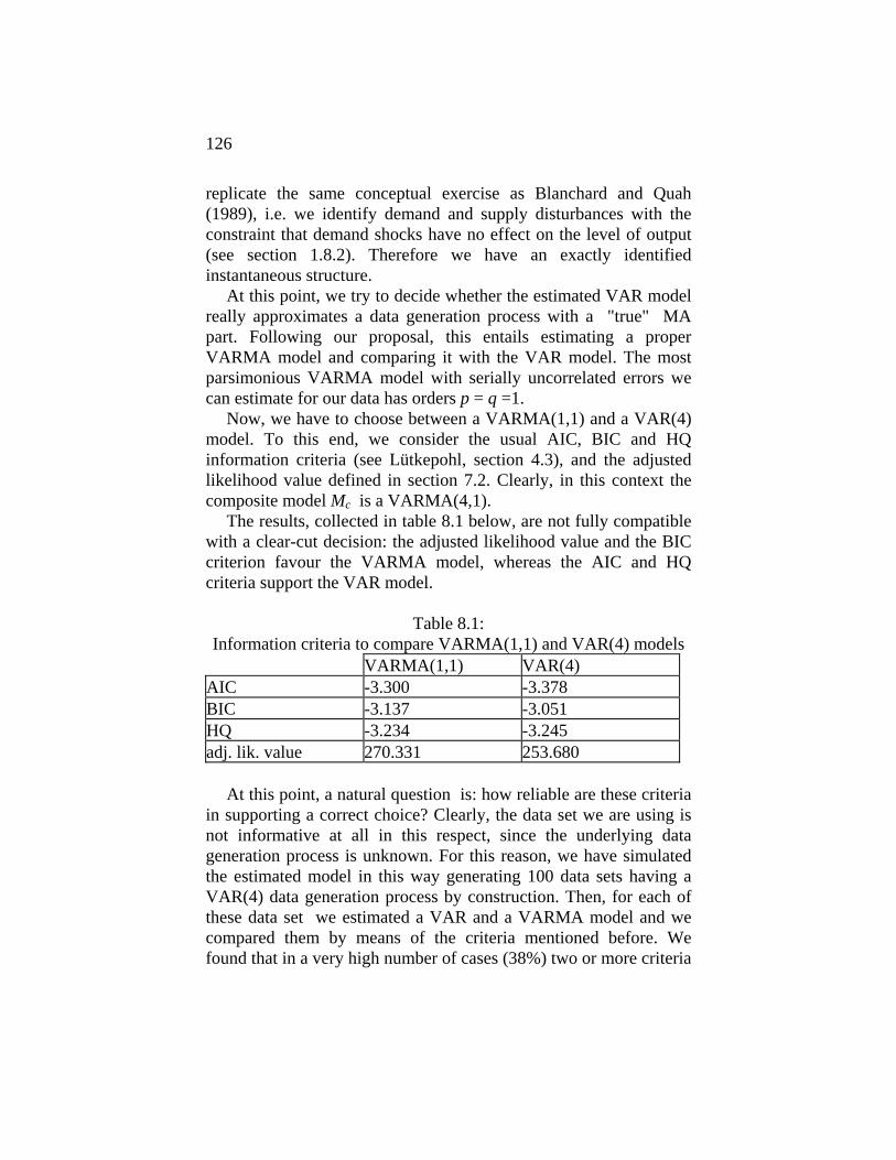
126
replicate the same conceptual exercise as Blanchard and Quah (1989), i.e. we identify demand and supply disturbances with the constraint that demand shocks have no effect on the level of output (see section 1.8.2). Therefore we have an exactly identified instantaneous structure.
At this point, we try to decide whether the estimated VAR model really approximates a data generation process with a "true" MA part. Following our proposal, this entails estimating a proper VARMA model and comparing it with the VAR model. The most parsimonious VARMA model with serially uncorrelated errors we can estimate for our data has orders p = q =1.
Now, we have to choose between a VARMA(1,1) and a VAR(4) model. To this end, we consider the usual AIC, BIC and HQ information criteria (see Lütkepohl, section 4.3), and the adjusted likelihood value defined in section 7.2. Clearly, in this context the composite model Mc is a VARMA(4,1).
The results, collected in table 8.1 below, are not fully compatible with a clear-cut decision: the adjusted likelihood value and the BIC criterion favour the VARMA model, whereas the AIC and HQ criteria support the VAR model.
Table 8.1:
Information criteria to compare VARMA(1,1) and VAR(4) models VARMA(1,1) VAR(4) AIC -3.300 -3.378 BIC -3.137 -3.051 HQ -3.234 -3.245 adj. lik. value 270.331 253.680
At this point, a natural question is: how reliable are these criteria
in supporting a correct choice? Clearly, the data set we are using is not informative at all in this respect, since the underlying data generation process is unknown. For this reason, we have simulated the estimated model in this way generating 100 data sets having a VAR(4) data generation process by construction. Then, for each of these data set we estimated a VAR and a VARMA model and we compared them by means of the criteria mentioned before. We found that in a very high number of cases (38%) two or more criteria

127
favour the VARMA model, although the true generation process is VAR(4). We must therefore conclude that in many applications the researcher has to be extremely cautious about the reliability of the model comparison stage.
In our view, this is a clear example of the risks connected with any model specification decision: when real data are analysed, there is no such thing as the "true" model, since models have to be considered as appropriate approximations of a complex reality.
Going back to our real data example, in figure 8.2 the estimated VAR roots are plotted in the complex plane. If one decided to use the Lippi and Reichlin criterion, it would be difficult to draw conclusive evidence in favour or against the presence of a genuine MA part, and about the modulus of its roots.
Figure 8.2: Estimated VAR roots
VAR(4) roots
-2-1.5
-1-0.5
0
0.51
1.52
-10 -5 0 5
real part
imag
inar
y pa
rt
Anyway, we proceed by estimating the VARMA(1,1) model via
maximum likelihood, and the resulting model is then identified by imposing the Blanchard and Quah (1989) constraint that demand shocks do not have long run effect on the level of output (see section 1.8.2 of this book). Therefore we obtain4:
4 In what follows all the symbols refer to estimated magnitudes. We avoid using the ^ symbol in order not to complicate the notation.

128
A(L) yt = P(L) et, et ~ VWN(0, In) Since in this particular application, the estimated MA roots are complex, we apply the two corresponding BMs to obtain:
A(L) yt = P* (L) vt*, vt
* ~ VWN(0, In) where both P*(L) and vt
* are complex. At this stage, we apply again the Blanchard-Quah identification and we obtain a real basic NFR:
A(L) yt = Q(L) vt, et ~ VWN(0, In) where Q(L) has roots which are reciprocal to those of P(L), and the Blanchard and Quah long run constraint is satisfied.
At this stage, we are ready to plot the impulse response functions of the basic VARMA(1,1) NFR and of its fundamental counterpart (see figures 8.2-8.5 at the end of this section). We report also the impulse response functions of the structural VAR(4) model.
From this example we can draw the following conclusions. Firstly, we can see that, at least in this application, there are not very substantial differences between impulse response functions of the fundamental and the non fundamental VARMA representations. We can notice differences only for the first four or five lags responses, whereas at longer horizons the impulses tend to coincide.
Secondly, the model choice aspect seems crucial: notice the differences between the VAR and the (fundamental or non-fundamental) VARMA impulse responses. These differences are substantial and persist in the long run for the responses to supply shocks.

129
Figure 8.2: response of gdp to a demand shock
Figure 8.3: Response of gdp to a supply shock
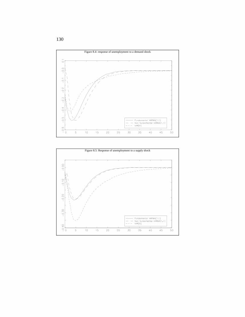
130
Figure 8.4: response of unemployment to a demand shock
Figure 8.5: Response of unemployment to a supply shock
131
Chapter 9 Two applications of Structural VAR analysis
In this chapter we present the results of two different applications of Structural VAR analysis, which are intended to provide the reader with some evidence of the way in which the techniques described in this book can be concretely applied.
The first of these two applications (section 9.1) is a modification of Blanchard's (1989) model which has already appeared on an international journal, and we will only describe its main methodological features. The second example, contained in section 9.2, deals with a set of Italian interest rates, and summarises the results contained in an unpublished paper written jointly by the two authors of this book with two other co-authors. We believe that this second exercise might be particularly useful to the reader, since it clarifies a series of implementation problems usually encountered by applied researchers. Moreover, the preparation of this exercise has given impulse to the creation of a RATS computer package for cointegration and structural analysis in VAR systems1. 9.1. A traditional interpretation of Italian macroeconomic fluctuations
In this section we describe the results of an application conducted by one of the authors of this book and documented in the paper "A traditional interpretation of macroeconomic fluctuations: the case of Italy" (Giannini, Lanzarotti and Seghelini,1995, henceforth GLS, 1995), where Blanchard’s (1989) Structural VAR model has been
1 We are referring to the MALCOLM package written by Rocco Mosconi (Politecnico di Milano),and already mentioned in the Foreword of this book. The package has been used extensively in the application contained in section 9.2, in order to carry out all the steps of the modelling procedure documented there. As for the availability of this package, see the indications contained in the Foreword of this book.
132
applied on Italian data and modified in order to obtain an over-identified structure2.
Let us just recall that Blanchard (1989) uses the “traditional” Keynesian model to analyse the US macroeconomic fluctuations, and that he analyses the vector series:
yt = [y1t , y2t , y3t , y4t , y5t ]' = [yt , ut , pt , wt , mt ]' where yt is the logarithm of real output, ut is the unemployment
rate, pt is the logarithm of price level, wt is the logarithm of nominal wage and mt is the logarithm of nominal money, whereas GLS (1995) study the Italian counterparts of Blanchard's series 3. The data are quarterly, seasonally adjusted and the sample period is 1970:1-1990:4. 9.1.1. The reduced form VAR model
The reduced form VAR model is A(L) yt = μ + εt , εt ~ VWN (0, Σ ) A(L) = I5 - A1L - A2L2 - A3L3 - A4L4
where the deterministic component is a vector of constant term. The lag order of the model (which is equal to 4) has been determined by requiring that the resulting model has serially uncorrelated residuals. Absence of serial correlation in the residuals has been verified by means of a multivariate version of the Godfrey test4.
Another important feature of the data that have been statistically checked is the fact that all the series in yt are difference-stationary, i.e. I(1). This has been verified by using standard unit root tests, such as the Perron and Phillips (1988) and Schmidt and Phillips (1992) tests. All tests details can be found in section 1 of GLS (1995).
This result has two consequences. Firstly, given that the VAR polynomial has unit roots, then the deterministic behaviour of each
2 In section 1.8.3 Blanchard's (1989) model has been briefly described in order to provide an example of an AB model. In Blanchard's context, two parameters, a34 and b12, had to be set equal to fixed values (and not estimated) in order to achieve exact identification. 3 For the sake of precision, in the Italian application -1/U is used in order to measure unemployment, where U is the total unemployment rate. This choice is justified at length in the paper. 4 See Godfrey 1988, p. 178.
133
series will be that of a linear trend, as documented in section 6.3.1 of this book. Secondly, there is the possibility that the I(1) series under study are cointegrated. 9.1.2. Cointegration properties
By using Johansen's testing procedure, GLS (1995) conclude that their vector series are cointegrated5, with cointegrating rank equal to 3. The three cointegrating relationships are given the following interpretation
β = − +
⎡
⎣
⎢⎢⎢⎢⎢⎢
⎤
⎦
⎥⎥⎥⎥⎥⎥
ββ
β β β βββ
11
23
31 42 52 33
42
52
1 00 0
0 11 0
( )
or, equivalently: mt = - β11 yt - β31 pt +z1t (long run monetary equilibrium) yt = - β42 (wt - pt ) - β52 (mt - pt ) +z2t (long run aggregate demand ) wt = - β23 ut - β33 pt +z3t (long run wage determination), zt = [z1t , z2t , z3t ]' ~ I(0) For the economic justification and the numerical estimates of the cointegration relationships, see GLS (1995), section 2.
From a more technical point of view, the above long-run relationships are obtained by specifying the following set of linear homogeneous restrictions on the columns of β = [β1, β2, β3]:
β1 = H1 φ1, β2 = H2 φ2, β3 = H3 φ3
5 See Table 2 in GLS (1995).

134
H1
1 0 00 0 00 1 00 0 00 0 1
=
⎡
⎣
⎢⎢⎢⎢⎢⎢
⎤
⎦
⎥⎥⎥⎥⎥⎥
, H2
1 0 00 0 00 1 10 1 00 0 1
= − −
⎡
⎣
⎢⎢⎢⎢⎢⎢
⎤
⎦
⎥⎥⎥⎥⎥⎥
, H3
0 0 01 0 00 1 00 0 10 0 0
=
⎡
⎣
⎢⎢⎢⎢⎢⎢
⎤
⎦
⎥⎥⎥⎥⎥⎥
plus a normalisation constraint on each column of β.
Following the approach described in section 6.3.3 of this book, Johansen's (1995b) theorem can be used to check that the constraints written above lead to an identified structure for the long run relationships6. Moreover, on the basis of the usual order conditions (we have three constraints for each of the three equations), one immediately concludes that the long run structure is exactly identified. Therefore no constraint is actually imposed on the cointegrating relationships parameter space. 9.1.3. Structural identification of instantaneous relationships
We refer to Blanchard's (1989) identification scheme for the instantaneous relationships, which has been explained in detail in section 1.8.3 of this book. In order to achieve exact identification, GLS (1995) add the following two homogeneous restrictions to the ones used by Blanchard:
a32 = 0 b12 =0
The first added constraint is to exclude instantaneous effects of p on w (in Sims' (1988) parlance, this is a minimal delay restriction), and is justified by the Keynesian hypothesis of wage stickiness. The second constraint does not have a theoretical justification, but emerges from statistical considerations: given the other added constraints described below and leading to a situation of over-identification, if one removed the constraint b12 = 0, an insignificant estimate for b12 would be obtained.
6 Johansen's theorem is implemented in the package MALCOLM.

135
Starting from the estimate of the resulting exactly identified structure, four free parameters were found insignificant and they were set equal to zero: a31= a51= a53 = b32 = 0 In addition to these, two constraints on the structured loading matrix were imposed (see section 6.3.4 of this book), by considering the Structural VAR model in its equivalent ECM form Γ*(L) yt = α* β' yt-1 + B et , Γ*(L) = A Γ(L), α* = A α The constraints on α*, the structured loading matrix, are intended to exclude that monetary disequilibrium errors (z1t ) directly enter the structural equations for wage and unemployment. Formally, these constraints can be written as (u2' A) ⋅ (α u1) (u4' A) ⋅ (α u1) where ui denotes the i-th column of I5. Notice that, given all the other constraints being specified so far, the two constraints on the structured loading matrix amount to set a21 and a42 to fixed values.
We would like to point out that the attempt to impose restrictions on the structured loading matrix and strongly sparse structures on the matrices A and B might give rise to conflicts. Sometimes such restrictions could lead to a system of inconsistent constraints.
At this point, the order condition for identification suggests that we are in the presence of an over-identified structure, with six over-identifying constraints. The rank condition was numerically checked and found to be supported by the structure of the constraints described above.
Therefore the over-identified model was estimated via maximum likelihood , and the validity of the over-identifying restrictions has been found to be supported by the data, by using the likelihood ratio test 7 described in chapter 4. 9.1.4. Dynamic simulation
The estimated structural model can be used for dynamic simulations. We do not report here the results of the structural
7 See Table 4 in GLS (1995).

136
impulse response analysis8, but we can see that they are consistent with the general Keynesian framework inspiring the model: aggregate demand shocks (e1) move output and prices in the same direction; price stickiness induces p to converge to the new equilibrium level with a significant delay. Striking results emerge from FEVD analysis. It is true that the variance of y in the short run is almost entirely explained by demand shocks, (as the standard Keynesian paradigm would predict). Nevertheless, in the long-run the real supply shocks (e2) do not assume a relevant role as the underlying economic theory would predict and it is found that the main driving force for y in the long run are the nominal shocks (e3 and e4). 9.2. The transmission mechanism among Italian interest rates
In this section, we summarise some of the results contained in the paper, "The transmission mechanism among Italian interest rates" (Amisano, Cesura, Giannini and Seghelini, 1995, henceforth ACGS, 1995), where a Structural VAR model is built for a set of Italian interest rates in order to investigate their dynamic interactions. The aim of this study is to analyse how monetary impulses propagate in the Italian monetary market.
The aim is accomplished by determining the long-run relationships, i.e. identifying the cointegration space, and modelling the instantaneous interactions. Then, dynamic simulations give the linkage between short and long run properties. The analysis emphasises the role of the rate on repurchasing operations of the Italian central bank; this seems to be the driving force of the Italian monetary market. 9.2.1. The choice of the variables In a VAR analysis of transmission mechanisms, the key problem is the choice of the set of variables. The choices made in
8 GLS(1995), section 4.

137
this respect are mainly guided by reflecting the institutional features of the Italian monetary market 9. In synthesis, the following five rates are taken into consideration: 1) PCT: the rate on repurchasing agreements between the central bank and credit institutions ("pronti contro termine" or PCT), intended as a policy rate. 2) RINT1M: the interbank rate on one-month operations. 3) RBOT3: the rate on three month Treasury bills ("Buoni Ordinari del Tesoro, or BOT) 4) ATTMIN: the minimum rate on bank loans. 5) PASMAS: the maximum rate on bank deposits All the series are nominal, the data are monthly and refer to the period 1982:01- 1992:08.
In a nutshell, the set of rates included in the analysis captures the way in which monetary shocks propagate: these shocks are immediately reflected by the PCT rate, affect the interbank rate and the Treasury bills rate, and (via the interbank rate) they finally reach the bank rates on loans and deposits.
As for the univariate properties of the series under study, the usual unit root tests clearly indicate that they are all I(1), and this feature is not surprising, given that the interest rates being considered are nominal and the underlying Italian inflation series can be modelled as a I(1) series for the sampling period being considered. The results of the Phillips and Perron (1988) integration tests are collected in Table 9.2.1 presented below.
9 For a detailed discussion of the motivations behind the choice of the rates being analyse, see section 1 of ACGS (1995).

138
9.2.2. The reduced form VAR model
The starting point of the multivariate analysis is the following reduced form VAR
A y D 0A I A A
( )( ) = ...1
L VWNL L L
t t t t
n pp
= + +
− − −
μ ψ ε ε , ~ ( , )Σ
where yt=[PCTt, RINT1Mt, RBOT3t, ATTMINt, PASMASt]’ and Dt is a set of eleven seasonal dummies variables. The presence of monthly seasonal dummies is strongly supported by a joint significance likelihood ratio test (χ2
[55] = 139.59, p-value=0.000). Seasonality was largely unexpected in an interest rates setting.
Nevertheless, seasonality is confirmed by univariate analysis of each series. The results of this analysis provide some elements which make it possible to connect the observed univariate seasonal patterns to some institutional features of the Italian monetary market11. As for the choice of the lag length of the VAR analysis, several different criteria have been used, such as the Hannan and Quinn (1979) information criterion, pointed out by Reimers (1993) as the most reliable in the presence of cointegration, and the classical LR tests (with a small sample correction suggested by Sims, 1980). The
10 5% size critical values are -13.70 and -2.89 for Z(α*) and Z(tα*) respectively. 11 In synthesis, seasonality seems to be connected to the strong intra-annual seasonal patterns of wage compensations (and therefore of households' liquidity) and in the public sector bonds issuing procedures. For a description of the univariate statistical procedures used and the institutional interpretation of interest rates seasonality, see section 2 and Appendix A in ACGS (1995).
Table 9.2.1 Phillips-Perron Integration Tests 10
Non-parametric corrections based on a window size =13, Series Z(α*) Z(tα*) PCT -7.78 -2.44 RINT1M -4.98 -2.24 RBOT3 -4.39 -2.60 PASMAS -1.97 -2.09 ATTMIN -3.23 -2.70

139
results, collected in table 9.2.2, give evidence in favour of a model with two lags.
Table 9.2.2:Lag Order Determination p* = 5, HQ=Hannan and Quinn Criterion
lag (h)
LR: L[p* ] vs. L[h ]
df p-va. LR: L[h ] vs. L[h-1]
df p-va. HQ
1 184.923 25 0.02 - - - -11.181 2 99.667 50 0.64 70.284 25 0.00 -11.236 3 56.564 75 0.85 33.782 25 0.11 -9.142 4 23.381 100 0.90 24.657 25 0.48 -8.434 5 - - - 16.424 25 0.90 -7.646
To provide further evidence, a multivariate version of the
Godfrey portmanteau test (see Godfrey, 1988) is performed, confirming two as an appropriate choice for lag length.
Table 9.2.3 Godfrey Portmanteau Test for the VAR(2)
correlations Godfrey test degrees of freed. p-value 1 34.384 25 0.100 1,2 54.787 50 0.301 9.2.3. Cointegration properties
The following step consists in conducting inference on the cointegration rank, on the basis of the maximum likelihood approach (see section 6.3). In this respect we have seen that the distributions of the rank statistics depend on the deterministic components in the VAR model; therefore one should jointly determine rank and the kind of deterministic polynomial. In the present case, dealing with interest rates, it is reasonable to consider a deterministic component of the kind: μ = αβ0. This choice implies the presence of an intercept term in the cointegration relationships and the absence of a linear trend in the levels of the series 12.
There is a strong a-priori on the cointegration rank: considering a set of nominal interest rates, the non-stationary driving force for all of them is likely to be the inflationary process. The hypothesis of 4 cointegrating vectors would be consistent with this view.
12 This corresponds to case 2) of section 6.3.1.

140
In Table 9.2.4 we present Johansen’s cointegrating rank statistics. The results are quite puzzling in suggesting rank equal to three at the usual 5% size. A deeper analysis of the properties of the model suggests not to take these results at face value.
Table 9.2.4
Johansen's Cointegration Rank Tests λ-maxi test: testing legitimacy of rank reduction from r+1 to r.
rank test 80% quantile
90% quantile
95% quantile
0 44.36 28.76 31.66 34.40 1 33.32 22.95 25.56 28.14 2 26.16 17.40 19.77 22.00 3 12.11 11.54 13.75 15.67 4 5.73 5.91 7.52 9.24
trace test: testing legitimacy of rank reduction from 5 to r. rank test 80%
quantile 90% quantile
95% quantile
0 121.78 66.91 71.86 76.95 1 77.32 45.65 49.65 53.12 2 44.00 28.75 32.00 34.91 3 17.84 15.25 17.85 19.96 4 5.73 5.91 7.52 9.24
Following Hansen and Johansen (1993) iterative procedure, the robustness of the rank results over the sample period is investigated. The outcome, presented in figure 9.2.1, suggests that the sampling evidence is not completely in favour of rank three. We ascribe this to the presence of a fourth cointegration relationship with particularly persistent residuals, which is not signalled by rank statistics unless the size of the test is increased.13 On this basis, in the sequel, we adopt rank four.
Figure 9.2.1 Hansen and Johansen Tests
13 On the interpretation of the fourth cointegrating vector we shall dwell at the end of this section.

141
Stability of the cointegration Rank: R-model (size = 5%)
87 88 89 90 91 920.00
0.25
0.50
0.75
1.00
1.25
1.50
1.75
Stability of the cointegration Rank: Z-model (size = 5%)
87 88 89 90 91 920.00
0.25
0.50
0.75
1.00
1.25
1.50
1.75
In the figure above we have presented the results of the recursive
estimation of models Z and R. In Hansen and Johansen (1993) parlance, models Z and R differ in that the former implies recursive estimation of all the parameters in the model, the latter of only the ones lying in the span of α . The above figures represent the cointegrating rank statistics, scaled by their respective critical values, recursively calculated in the second part of the sample period. Therefore, the number of lines above the value of one gives the outcome of the rank test evaluated for any partial sample period.

142
As for the structural interpretation of the cointegrating relationships, following the approach described in section 6.3.3, we consider the hypothesis that interest rate spreads are stationary. This interpretation of the cointegrating relationships can be achieved by specifying the following set of homogeneous linear constraints on the four columns of
β* = [β1*, β2
*, β3*, β4
* ] = [β', β0']' β1 = H1 φ1 , β2 = H2 φ2 , β3 = H3 φ3 , β4 = H4 φ4
H1
1 01 00 00 00 00 1
=
−⎡
⎣
⎢⎢⎢⎢⎢⎢⎢
⎤
⎦
⎥⎥⎥⎥⎥⎥⎥
, H 2
1 00 01 00 00 00 1
=
−⎡
⎣
⎢⎢⎢⎢⎢⎢⎢
⎤
⎦
⎥⎥⎥⎥⎥⎥⎥
, H 3
0 01 0
0 01 00 00 1
=
−⎡
⎣
⎢⎢⎢⎢⎢⎢⎢
⎤
⎦
⎥⎥⎥⎥⎥⎥⎥
, H 4
0 00 00 01 0
1 00 1
=−
⎡
⎣
⎢⎢⎢⎢⎢⎢⎢
⎤
⎦
⎥⎥⎥⎥⎥⎥⎥
plus a normalisation constraint on each column of β*.
Following the approach described in section 6.3.3 of this book, Johansen's (1995b) theorem can be used to check that the constraints written above lead to an identified structure for the long run relationships. Moreover, on the basis of the usual order conditions (we have five constraints for each of the four cointegrating equations), the long run structure is over identified with four over-identifying constraints imposed on the parameter space of the cointegrating relationships. The validity of these constraints is checked by means of a χ2
[4] distributed likelihood ratio test. The estimated cointegration vectors are presented below, in Table
9.2.5: Table 9.2.5.
Cointegrating Vectors (t-statistics in brackets) RINT M PCT z1 0 752
2 61 1− = +.( . )
RBOT PCT z3 0 5091 49 2− = − +
−.
( . ) ATTMIN RINT M z− = +1 0 533
4 23 3.( . )
PASMAS ATTMIN z− = − +−2 774
24 44 4.( . )

143
(LR test for over-identification: squared[4]=8.655, p-value = 0.07) The reported t-statistics are obtained on the basis of the
asymptotic distribution of the over-identified cointegrating vectors, as described in section 6.3.4.
Clearly, that reported above is only one of the possible ways of writing the cointegrating relationships as to imply spreads stationarity; this one allows clear connections between markets, which are regarded as neighbouring from the point of view of daily activity of financial intermediaries.
Moreover, in this particular interpretation of the cointegration space, the ATTMIN-PASMAS spread is written explicitly; looking at figure 9.2.2, one can notice that this spread has a particularly persistent behaviour and, in our interpretation, it is responsible for the ambiguity in the rank test results.
Figure 9.2.2 Residuals from cointegrating vector: PASMAS ATTMIN z− = − +
−2 774
24 44 4.( . )
82 83 84 85 86 87 88 89 90 91 92-1.5
-1.0
-0.5
0.0
0.5
1.0
1.5
2.0
9.2.4. Structural identification of instantaneous relationships
In this section we describe how to organise the instantaneous correlations between the variables, which have been hidden so far in the covariance matrix of the reduced form disturbances (Σ).
An AB- model is chosen: A A(L) yt = B et , et ~ VWN(0, I5)

144
Obviously, the identification of the structure requires a set of constraints based either on theoretical or “minimum delay” zero restrictions (see Sims, 1988).
In the context of the ACGS (1995) model, the et disturbances are interpreted as idiosyncratic shocks and, not having any a-priori about their interactions, the structural effort is limited to the interactions among the observable shocks, i.e. to the instantaneous correlations of the observable variables. Thus we have a diagonal B matrix14, whose task is only to normalise the variances of the structural innovations et to one.
The final structure of the instantaneous equations (presented in figure 9.2.3 and in table 9.2.6) has been obtained starting from an exactly identified model, i.e. from the lower triangular Choleski decomposition of Σ, which seemed to suit well the scheme of the transmission mechanisms within the month across the interest rates being considered. Then, by deleting the non-significant parameters in the just-identified A matrix, a situation of over-identification is reached. The validity of the constraints has been checked by a likelihood ratio test.
In this way it is possible to investigate the possible presence of significant parameters above the diagonal of A, corresponding to intra-monthly feedbacks running from the lower elements in the ordering to the upper ones.
Figure 9.2.3
Instantaneous linkages
14 This model differs from a K-model since here B is diagonal, not equal to the identity matrix.
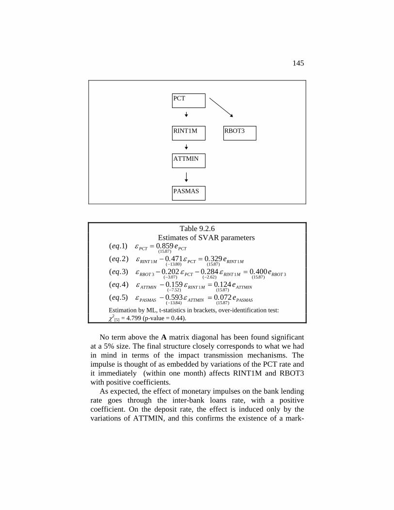
145
PCT
RINT1M
ATTMIN
PASMAS
RBOT3
Table 9.2.6 Estimates of SVAR parameters
( . ) .
( . )eq ePCT PCT1 0 859
15 87ε =
( . ) . .
( . ) ( . )eq eRINT M PCT RINT M2 0 471 0 3291 13 80 15 87 1ε ε− =
−
( . ) . . .
( . ) ( . ) ( . )eq eRBOT PCT RINT M RBOT3 0 202 0 284 0 4003 3 07 2 62 1 15 87 3ε ε ε− − =
− −
( . ) . .
( . ) ( . )eq eATTMIN RINT M ATTMIN4 0 159 0 124
7 52 1 15 87ε ε− =
−
( . ) . .
( . ) ( . )eq ePASMAS ATTMIN PASMAS5 0 593 0 072
13 84 15 87ε ε− =
− Estimation by ML, t-statistics in brackets, over-identification test: χ2
[5] = 4.799 (p-value = 0.44). No term above the A matrix diagonal has been found significant
at a 5% size. The final structure closely corresponds to what we had in mind in terms of the impact transmission mechanisms. The impulse is thought of as embedded by variations of the PCT rate and it immediately (within one month) affects RINT1M and RBOT3 with positive coefficients.
As expected, the effect of monetary impulses on the bank lending rate goes through the inter-bank loans rate, with a positive coefficient. On the deposit rate, the effect is induced only by the variations of ATTMIN, and this confirms the existence of a mark-

146
down cost setting mechanism, which is typical in context with oligopsonistic market power 15. 9.2.5. Dynamic simulation
We present some selected results taken from the whole set of dynamic simulations obtained by means of the model so far described. The simulations are calculated for 36 periods (3 years).
As for the impulse responses, we present only the responses to the structural shocks on PCT, i.e. the "policy" shocks, which are graphed in figure 9.2.4, with the 90% confidence bounds based on the asymptotic distributions of the structured impulse responses, as explained in sections 5.1 and 6.3.4 of this book.
15 See ACGS (1995), section 3.2 for a detailed interpretation of these findings.

147
Figure 9.2.4 Responses of the series to a structural shock in PCT equation
response of PCT
1 4 7 10 13 16 19 22 25 280.0
0.2
0.4
0.6
0.8
1.0
1.2
1.4
response of RINT1M
1 4 7 10 13 16 19 22 25 280.0
0.2
0.4
0.6
0.8
1.0
1.2
1.4
response of RBOT3
1 4 7 10 13 16 19 22 25 280.0
0.2
0.4
0.6
0.8
1.0
1.2
1.4

148
response of ATTMIN
1 4 7 10 13 16 19 22 25 280.0
0.2
0.4
0.6
0.8
1.0
1.2
response of PASMAS
1 4 7 10 13 16 19 22 25 280.00
0.16
0.32
0.48
0.64
0.80
0.96
1.12
Given the structural interpretation, we read a positive shock in
terms of a contraction of resources available through temporary re-purchase operations. The effects are positive, significant and persistent for all the series in the system, and at any horizon.
As for the FEVD analysis, in Table 9.2.7 we present the percentage of the variance of each series explained by structural innovations in PCT (top panel), and the percentage of PCT variance explained by the different structural shocks (bottom panel). These coefficients have been computed for different horizons and are accompanied by t-statistics obtained on the basis of the FEVD asymptotic distributions (see sections 5.2 and 6.3.4 of this book).
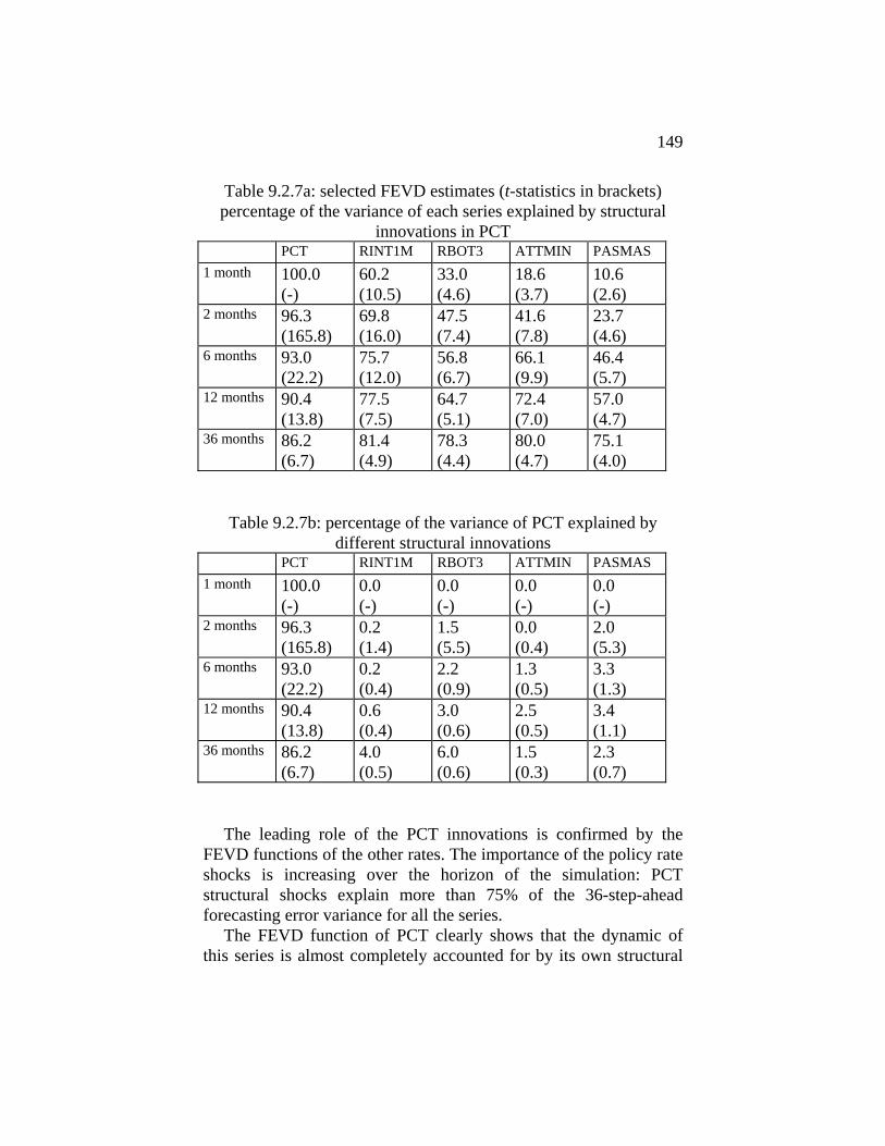
149
Table 9.2.7a: selected FEVD estimates (t-statistics in brackets) percentage of the variance of each series explained by structural
innovations in PCT PCT RINT1M RBOT3 ATTMIN PASMAS 1 month 100.0
(-) 60.2 (10.5)
33.0 (4.6)
18.6 (3.7)
10.6 (2.6)
2 months 96.3 (165.8)
69.8 (16.0)
47.5 (7.4)
41.6 (7.8)
23.7 (4.6)
6 months 93.0 (22.2)
75.7 (12.0)
56.8 (6.7)
66.1 (9.9)
46.4 (5.7)
12 months 90.4 (13.8)
77.5 (7.5)
64.7 (5.1)
72.4 (7.0)
57.0 (4.7)
36 months 86.2 (6.7)
81.4 (4.9)
78.3 (4.4)
80.0 (4.7)
75.1 (4.0)
Table 9.2.7b: percentage of the variance of PCT explained by different structural innovations
PCT RINT1M RBOT3 ATTMIN PASMAS 1 month 100.0
(-) 0.0 (-)
0.0 (-)
0.0 (-)
0.0 (-)
2 months 96.3 (165.8)
0.2 (1.4)
1.5 (5.5)
0.0 (0.4)
2.0 (5.3)
6 months 93.0 (22.2)
0.2 (0.4)
2.2 (0.9)
1.3 (0.5)
3.3 (1.3)
12 months 90.4 (13.8)
0.6 (0.4)
3.0 (0.6)
2.5 (0.5)
3.4 (1.1)
36 months 86.2 (6.7)
4.0 (0.5)
6.0 (0.6)
1.5 (0.3)
2.3 (0.7)
The leading role of the PCT innovations is confirmed by the FEVD functions of the other rates. The importance of the policy rate shocks is increasing over the horizon of the simulation: PCT structural shocks explain more than 75% of the 36-step-ahead forecasting error variance for all the series.
The FEVD function of PCT clearly shows that the dynamic of this series is almost completely accounted for by its own structural

150
innovations. This is interpreted as evidence of strict exogeneity, as indicated in Sims (1980), and Bernanke and Blinder (1992). This result, together with the indications coming from impulse response analysis, is a key point in supporting the interpretation that the PCT rate reflects policy impulses.
Another important point is the absence of significant feedbacks from the other rates to PCT. There is no logical a-priori reason to exclude effects of this sort for the policy rate; it is simply believed that they are overwhelmed by the importance of the PCT structural innovations. In fact, looking at table 9.2.7, there are small but significant FEVD coefficients of PCT associated with RBOT3 and PASMAS shocks in the very short run (2 or 3 steps). 9.2.6. The Lippi-Reichlin criticism
As we have seen in chapter 8 of this book, the validity of the dynamic simulation results of a Structural VAR model is questioned by the Lippi and Reichlin (1993, 1995) criticism, connected to the problem of non fundamental representations.
With regard to this particular application, as mentioned in section 8.3, we believe that there is an easy way to demonstrate that the Lippi and Reichlin argument does not apply in this specific case, since we can cautiously rule out the presence of a genuine moving average part. In fact, following the Lippi and Reichlin (1994) rule-of-thumb approach described in section 8.3, the estimated VAR roots, obtained via state space representation of the system are graphed in the complex diagram in figure 9.2.5.
The position of the VAR roots in the diagram appears very far from that implied by the presence of an MA component. Moreover, since the lag order of the VAR (p =2) is very low, it seems very unlikely that the VAR model can appropriately approximate a genuine MA part. For these reasons it is believed that the Lippi and Reichlin criticism can be considered as irrelevant in this particular applied context.

151
Figure 9.2.5 Complex diagram: estimated VAR roots.
-5
-4
-3
-2
-1
0
1
2
3
4
5
-5 -4 -3 -2 -1 0 1 2 3 4

151
ANNEX 1 The notions of reduced form and structure in Structural VAR modelling
Following Sims (1986) the present Annex attempts to illustrate the particular notions of structure in Structural VAR Analysis. The notions of structure, identification and reduced form are deeply connected in any econometric approach. In Structural VAR Analysis the reduced form of a vector y t of economic variables is simply represented by a vector autoregression of the type: ( )A yL t t = ε ( )A I A AL L Lp
p= − 1 K and ε t is a vector normal white noise with ( )E t tε ε Σ ' = The first stage of Structural VAR Analysis is the estimation of the reduced form. At this stage one can impose no theoretical a-priori constraint (apart from the number and type of economic variables included in the yt vector) . Thus unconstrained VAR Analysis can be seen as nothing more than a convenient way of organising the correlations between the variables of interest.
There is no reason to leave the first stage at this level of generality. For example, think of the problem of non stationarity and cointegration. Cointegration is a property of the data and if the so called "cointegration space" is not subject to structural interpretation, cointegration pertains only to statistics, not to economic theory.
Inserting cointegration constraints in a VAR in levels is only a way to arrive at a reduced form that "better" summarises the correlations between the variables under study ("better" should be understood as "more efficiently").
In the first stage of Structural VAR Analysis one may decide to move further on; the notion of non causality, obviously unlike the problem of imposing direction to instantaneous causality, is still a property concerning a subset of variables in yt , which may be detected on the basis of reduced form estimation. In this sense non-causality (as was the case for cointegration) is a property of the data
152
and not of any economic theoretical model. In the first stage, then, non-causality restrictions can be used to obtain reduced forms that "better" summarise the correlation between variables. Obviously, a number of other considerations should be used to extend the restrictions on the reduced form in the first stage and find more efficient reduced form representations.
Let us assume for simplicity that the first stage of Structural VAR Analysis could end with an estimate of the parameters of an unrestricted reduced form ( )A yL t t= ε , ( )E t tε ε Σ ' = obtaining estimates of A A1K p as $ $A A1K p ( )$ $ε t tL= A y
$ $ $ 'Σ =
ε εt t
t
T
T
=∑
1
In VAR Analysis the only source of variation of y t variables (apart from hypothetical changes in initial conditions or changes in a vector of deterministic part) are random shocks that in the reduced form are represented by a vector white noise ε t . The vector of unobservable ε t variables, often called vector of innovations or vector of surprise variables, can also be seen as the vector of unexplained random variations obtained as a residual from the projection of y t vector over its possibly infinite past (truncated at p by virtue of plausible approximation rules). In the ε t vector of unobservable variables one can expect substantial amount of contemporaneous correlation - not necessarily due to problems connected to temporal aggregation - which gives rise to a "theoretical" variance covariance matrix of ε t , Σ , typically not diagonal.
Structural VAR Analysis focuses its structural effort onto the organisation of instantaneous correlation between innovation variables. In the most general model studied in this book (the AB-model) the ε t vector must satisfy the following set of conditions: A Beε t t= A e B invertible matrices of order n ( )E tε = 0 ( )E t t ne e I′ = so
153
A A BBΣ ′ = ′ The vector of e t variables is a vector of orthonormal random
variables whose components are equal in number and corresponding in content to the list of variables contained in the y t vector and can be thought of as independent unit variance random shocks of the corresponding yit variables. These independent unit variance random shocks can be considered the ultimate independent source of variation of the y t variables.
With information contained in the estimated variance covariance matrix of the unrestricted reduced form, $Σ , and an appropriate number (and form) of a-priori restrictions on matrices A and B (together with some normalisation restrictions) one can presumably arrive at the conditions for unique identification of the A and B matrices. In this case the structural form of the VAR model becomes ( )A y Be∗ =L t t where ( ) ( )A AA∗ =L L
This structural form, on the basis of its parameters (once estimated), can be used to examine the path of estimated effects of (unit) changes (shocks) in the vector e t of independent zero mean variables. In the words of Hurwicz (1962) the equation ( )A y Be∗ =L t t is in structural form with respect to modifications of e t . Obviously this structural form has behavioural content if the A and B matrices contain the supposed "true" agents' behaviour in response to modifications of the e t vector.

154
ANNEX 2 Some considerations on the semantics, choice and management of the K, C and AB-models
This annex is devoted to illustrating our point of view on the significance of each type of model in relation to its corresponding set of identifying restrictions. The discussion may shed new light on the problem of which model to choose for specific applications. The present annex also includes some considerations on the "overall" working of the three models.
One point may need to be clarified beforehand, though. The AB-model, the most general of the three, may be cast in a K-model form by writing K B A1= − or in a C-model form by writing C A B1= −
Moreover, the K-model could be seen as a C-model (and vice-versa) if one noted that K C 1= − and C K 1= −
We will call "genuine" K, C and AB-models, the models which allow us to reach identification through a set of linear constraints of the type: R K dk kvec = R C dc cvec =
R A dR B d
a a
b b
vecvec
==
⎧⎨⎩
respectively. The transformation of "genuine" K, C or AB-models into models
of the C and K type in general give rise to a set of very complicated non linear restrictions with respect to the coefficients of the C and K matrices of the transformed models. Such restrictions can not be dealt with within the framework put forward in the present book; therefore only "genuine" models can be discussed in the set-up we propose.
Looking at different models and starting from the autoregressive representation of the so called first stage

155
( )A yL t t= ε ( )A I0 = n ( )E t tε ε Σ′ = the matrices K, C, A, and B operate in the following way within the above mentioned system: ( )K A y e L t t= for the K-model ( )A y CeL t t= for the C-model ( )A A y Be L t t= for the AB-model with ( )E t t ne e I′ =
In the K-model, matrix K directly applies to vector y t of observable quantities. Instantaneous correlations between observable variables are organized through the structure of the K matrix. On the contrary, instantaneous correlations between the unobservable quantities contained in the e t shocks vector can in no way be directly organised in the K-model.
In the C-model, matrix C directly applies to vector e t of unobservable quantities. Instantaneous co-movements of y t observable variables are indirectly organised since they result as linear combinations of a vector of independent shocks. Instantaneous co-movements of observable variables contained in the y t vector can in no way be directly organised in the C-model.
In the AB-model, matrices A and B apply to observable and unobservable quantities respectively. Thus the greatest flexibility is assured.
In order to tackle the problem of which model to choose in concrete applications, the first question that the researcher must face is whether the concrete problem under study admits a plausible formulation in terms of "genuine" K, C or AB models as defined in this annex.
The K-model is central in this book almost exclusively for analytical purposes. It could be better understood when regarded as the result of the transformation of a particular AB-model with ones on the A matrix main diagonal and (positive) elements only on the B matrix diagonal. In this way, also the K matrix K B A1= −

156
would have positive diagonal elements and exclusion restrictions on the coefficients of matrix A (i.e. zero values for the corresponding elements) would not change their positions in the K matrix.
In the K-model, apart from restrictions imposed on the positive diagonal (Kii) elements, the presence of a Kij (i j≠ ) coefficient different from zero results from a combination of theoretical and common sense considerations.
Every economic theory generally assumes the so called "logical time" but in our context we will consider real time. Thus causal relationships derived from economic theory (e.g. a causal relation linking variable j to variable i) can hold "instantaneously" only if they operate in the sampling period we are dealing with.
In other words, taking into account what Sims (1988) calls "minimum delay restrictions", a "logical-time" causal relation is a necessary but not sufficient condition for the corresponding kij coefficient to be different from zero.
In general, using the K-model and looking at an unchanged set of variables, one can expect that the progressive shortening of the sample period produces a corresponding progressive deletion of extradiagonal elements of the K matrix.
The K-model turns out to be particularly useful if economic theory can provide the researcher with some indication on the magnitudes of some total multipliers on observable variables. In this way, the considerations contained in section 6.1 could be used to achieve identification.
At first glance, the C-model looks less appealing as regards theoretical and common sense justifications of the organisation of observable variables' co-movements. In fact, C-models look particularly useful when long run constraints have to be imposed (such as neutrality conditions), often supposed to be valid in some actual economic contexts. For example, suppose that the vector y t is obtained by differentiating a vector (x t ) of I(1) non cointegrated variables and that y t possesses the usual (stable) autoregressive representation ( )A yL t t= ε ( )A xL t t Δ = ε

157
the stable ( )A L polynomial matrix can be inverted so to move to the equivalent Wold representation ( )Δx Ct tL= ε
Taking into account that in the C-model ε t t= C e we can write ( )Δx C C et tL= where the vector e t should contain the shocks which are similar in nature and ordering to the elements of the Δxt vector.
In order to identify C in a "genuine" C-model set-up, apart from a number of zero constraints on the C-matrix off-diagonal elements, we might impose some long run restrictions derived from the analysis of ( ) ( )C C C∗ =1 1 where ( )C∗ 1 is the matrix containing the "structured" multipliers of the elements of the e t shocks vector in relation to the elements of the Δxt vector. Let us suppose we wanted to impose a neutrality constraint such as the following: the level of the ith variable remains unchanged in the long run in response to movements of the jth variable. In this case, we should only constrain to zero the ( )cij
∗ 1 element of the ( )C∗ 1 matrix, which is tantamount to say that an independent shock to the variable j has a zero total effect on the change of the variable i. As a consequence, integrating the difference, we could see that a shock in the variable j does not affect the level of the variable i. This and other long-run restrictions could easily be accommodated in our "genuine" C-model with constraints of the form R C dc cvec = (see, for example, Shapiro and Watson 1988 and Blanchard e Quah 1989 for the use of C-models with constraints of this type). The AB-model's characteristic flexibility makes it the most promising in a number of applications, with a warning. The aforementioned long-run restrictions put on models K and C cannot be incorporated in the "genuine" AB-model because they correspond to complex non-linear constraints in the AB-model.

158
In chapter 9, we provide two examples of how to specify an AB-model in a cointegrated set up. However one should not forget that achieving identification of the K, C and AB-models is only the first step in Structural VAR model analysis. The second step consists in estimating the parameters of the chosen "genuine" model. After the estimation, one should first check that all estimate parameters are statistically significant and, if this is the case, that their signs and magnitudes are economically plausible. Moreover, in the case of overidentification, one should make sure that overidentifying restrictions are accepted by the data.
If estimation produces satisfactory results, the final step is dynamic simulation analysis carried out with instruments such as impulse response analysis and forecast error variance decomposition analysis. Only at this step one can fully appreciate the overall working of a Structural VAR model.
Not surprisingly, this last step can produce strikingly contrasting results, especially for what regards the congruence of the economic theory subsumed in the identification step and, at times, from the point of view of sound economic judgement. This situation can indeed arise looking at the fact that unstructured VAR modelling (representing the first stage of Structural VAR strategy) is independent of prejudices or supposedly "true" economic knowledge used in the identification step of the "genuine" K, C or AB-model chosen. In SVAR dynamic simulation analysis a somehow arbitrary theoretical structure has to be combined with a plausibly "true" model of the data: their mix does not necessarily make a good tasting cake. In this case, a researcher must go back to the first step and look for more plausible "genuine" models. From a statistical point of view, the problem of choice among alternative structuralisations of the same unstructured VAR model, as explained in chapter 7 of this book, can reasonably be posed only for models that yield satisfactory results after the third step has been carried out.
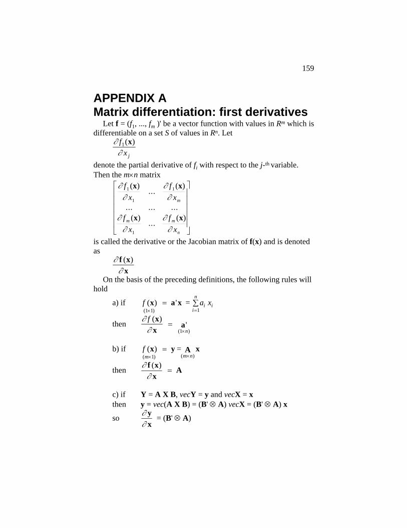
159
APPENDIX A Matrix differentiation: first derivatives
Let f = (f1, ..., fm )' be a vector function with values in Rm which is differentiable on a set S of values in Rn. Let
∂∂
fx j
1( )x
denote the partial derivative of fi with respect to the j-th variable. Then the m×n matrix
∂∂
∂∂
∂∂
∂∂
fx
fx
fx
fx
m
m m
n
1
1
1
1
( )...
( )
... ... ...( )
...( )
x x
x x
⎡
⎣
⎢⎢⎢⎢⎢
⎤
⎦
⎥⎥⎥⎥⎥
is called the derivative or the Jacobian matrix of f(x) and is denoted as
∂∂ f x
x( )
On the basis of the preceding definitions, the following rules will hold
a) if ( )( ) '
1 1 1× == ∑f a xi i
i
nx a x =
then ∂∂
(1 )
fn
( )'
xx
a=×
b) if
( ) ( )( )
m m nf
× ×=
1x y A x =
then ∂∂
f x
xA( )
=
c) if Y = A X B, vecY = y and vecX = x then y = vec(A X B) = (B' ⊗ A) vecX = (B' ⊗ A) x
so ∂∂
yx
= (B' ⊗ A)

160
d) vec
( )n n×X = vecX'
∂∂
vecvec
XX'
= OT
OT 2 = In2 , OT ' = OT = OT -1
(see Pollock, 1979, p.72) e) if Y = X-1
taking differentials (see Magnus and Neudecker, 1988) dY = -X-1(dX) X-1 and vectorising: vec(dY) = -(X'-1⊗X-1) vec(dX)
∂∂
( ) ( )
vecvec
XX'
= -(X'-1⊗X-1)
f) Chain rule (Pollock, 1979)
If u = u(y) is a vector function of y and y = y(x) is a function of a vector x, so that u = u[y(x)], then
∂∂
∂∂
∂∂
=
ux
uy
yx
⋅
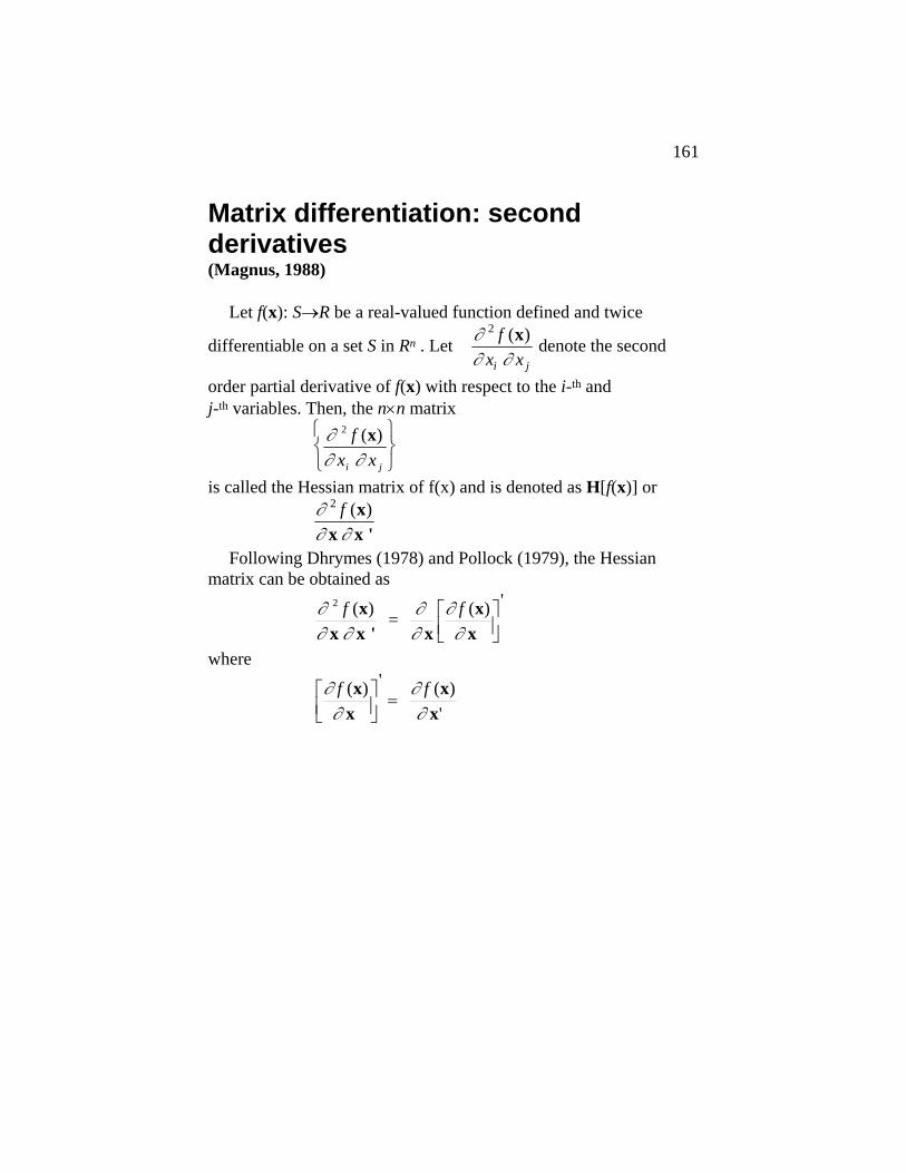
161
Matrix differentiation: second derivatives (Magnus, 1988)
Let f(x): S→R be a real-valued function defined and twice
differentiable on a set S in Rn . Let ∂∂ ∂
2 fx xi j
( )x denote the second
order partial derivative of f(x) with respect to the i-th and j-th variables. Then, the n×n matrix
∂∂ ∂
2 fx xi j
( )x⎧⎨⎩
⎫⎬⎭
is called the Hessian matrix of f(x) and is denoted as H[f(x)] or
∂∂ ∂
2 f ( )xx x '
Following Dhrymes (1978) and Pollock (1979), the Hessian matrix can be obtained as
∂∂ ∂
∂∂
∂∂
=
2 f f( ) ( ) 'xx x ' x
xx
⎡⎣⎢
⎤⎦⎥
where
∂∂
∂∂
f f( ) ' ( )'
xx
xx
⎡⎣⎢
⎤⎦⎥=
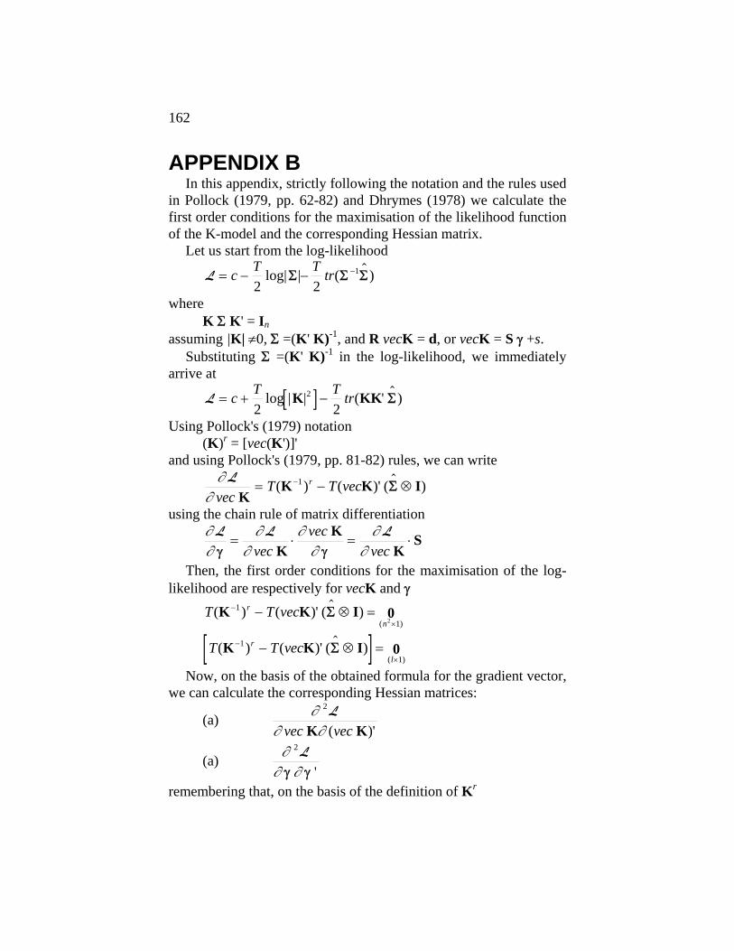
162
APPENDIX B In this appendix, strictly following the notation and the rules used
in Pollock (1979, pp. 62-82) and Dhrymes (1978) we calculate the first order conditions for the maximisation of the likelihood function of the K-model and the corresponding Hessian matrix.
Let us start from the log-likelihood
L = − − −c T T tr2 2
1log| | ( $ )Σ Σ Σ
where K Σ K' = In assuming |K| ≠0, Σ =(K' K)-1, and R vecK = d, or vecK = S γ +s.
Substituting Σ =(K' K)-1 in the log-likelihood, we immediately arrive at
[ ]L = + −c T T tr2 2
2log | | ( ' $ )K KK Σ
Using Pollock's (1979) notation (K)r = [vec(K')]' and using Pollock's (1979, pp. 81-82) rules, we can write
∂∂
Lvec
T T vecr
KK K I= − ⊗−( ) ( )' ( $ )1 Σ
using the chain rule of matrix differentiation
∂∂
∂∂
∂∂
∂∂
L L Lγ γ
= ⋅ = ⋅vec
vecvecK
KK
S
Then, the first order conditions for the maximisation of the log-likelihood are respectively for vecK and γ
T T vecr
n( ) ( )' ( $ )
(K K I 0−
×− ⊗ =1
1)2Σ
[ ]T T vecr
l( ) ( )' ( $ )
(K K I 0−
×− ⊗ =1
1)Σ
Now, on the basis of the obtained formula for the gradient vector, we can calculate the corresponding Hessian matrices:
(a) ∂∂ ∂
(
2Lvec vecK K)'
(a) ∂∂ ∂
2Lγ γ '
remembering that, on the basis of the definition of Kr

163
(K-1)r = {vec[(K-1) ']}' the gradient vector
∂∂
Lvec K
can be re-written in the following way
∂∂
{[ [( )' ]}'-1Lvec
T vec T vecK
K K I= − ⊗( )' ( $ )Σ
Following Dhrymes (1978), we can calculate the Hessian matrix as
H K
K K K K
K K
( )( )( )'
'
)'
vecvec vec vec vec
vec vec
= ⎛⎝⎜
⎞⎠⎟
=⎛⎝⎜
⎞⎠⎟
∂∂ ∂
∂∂
∂∂
∂∂
∂∂
=
(
2L L L
L L
∂∂
(
Lvec
T vec T vecK
K I K)'
( ' ) ( $ )( )= − ⊗−1 Σ
and then
( )H K
K KK
KI
( )( )( )'
( ' ) $
vecvec vec
T vecvec
T
=
− ⊗−
∂∂ ∂
∂∂
=
2L
1
Σ
Let us concentrate on the first member of the last expression. Using the chain rule, we can write
∂∂
∂∂
∂∂
(
vecvec
vecvec
vecvec
( ' ) ( ' )' )
( ' )KK
KK
KK
− −
= ⋅1 1
Using the rules introduced in Appendix A (see Pollock 1979, p. 81), we can write
[ ]∂∂
vecvec
( ' ) ( ' )KK
K K−
− −= − ⊗ ⋅1
1 1 OT
so we can arrive at
H K( )vec = ∂∂ ∂
2L
( ) ( )'vec vecK K
= -T{[ K K− −⊗1 1( ' ) ]⋅OT +( $Σ ⊗ I )}

164
Remembering that vecK = S γ + s is an affine function (see Theorem 11 in Magnus and Neudecker, 1988, p.112), the following Hessian matrix with respect to γ is simply
H( )'
γγ γ
=∂
∂ ∂
=
2L S' H(vecK) S
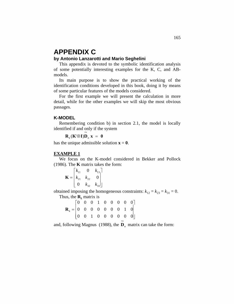
165
APPENDIX C by Antonio Lanzarotti and Mario Seghelini
This appendix is devoted to the symbolic identification analysis of some potentially interesting examples for the K, C, and AB-models.
Its main purpose is to show the practical working of the identification conditions developed in this book, doing it by means of some particular features of the models considered.
For the first example we will present the calculation in more detail, while for the other examples we will skip the most obvious passages. K-MODEL
Remembering condition b) in section 2.1, the model is locally identified if and only if the system
R K I D x 0k n( ' )~
⊗ = has the unique admissible solution x = 0. EXAMPLE 1
We focus on the K-model considered in Bekker and Pollock (1986). The K matrix takes the form:
K =⎡
⎣
⎢⎢⎢
⎤
⎦
⎥⎥⎥
k kk k
k k
11 13
21 22
32 33
00
0
obtained imposing the homogeneous constraints: k12 = k23 = k31 = 0. Thus, the Rk matrix is
Rk =⎡
⎣
⎢⎢⎢
⎤
⎦
⎥⎥⎥
0 0 0 1 0 0 0 0 00 0 0 0 0 0 0 1 00 0 1 0 0 0 0 0 0
and, following Magnus (1988), the ~Dn matrix can take the form:
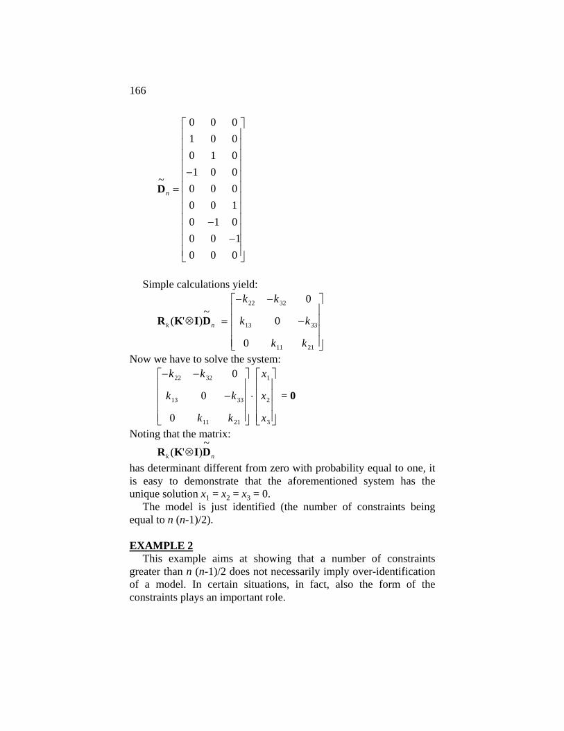
166
~Dn =
−
−−
⎡
⎣
⎢⎢⎢⎢⎢⎢⎢⎢⎢⎢⎢⎢
⎤
⎦
⎥⎥⎥⎥⎥⎥⎥⎥⎥⎥⎥⎥
0 0 01 0 00 1 01 0 0
0 0 00 0 10 1 00 0 10 0 0
Simple calculations yield:
R K I Dk n( ' )~
⊗ =
− −
−
⎡
⎣
⎢⎢⎢⎢
⎤
⎦
⎥⎥⎥⎥
k k
k k
k k
22 32
13 33
11 21
0
0
0
Now we have to solve the system:
− −
−
⎡
⎣
⎢⎢⎢⎢
⎤
⎦
⎥⎥⎥⎥
⋅
⎡
⎣
⎢⎢⎢⎢
⎤
⎦
⎥⎥⎥⎥
k k
k k
k k
x
x
x
22 32
13 33
11 21
1
2
3
0
0
0
= 0
Noting that the matrix: R K I Dk n( ' )
~⊗
has determinant different from zero with probability equal to one, it is easy to demonstrate that the aforementioned system has the unique solution x1 = x2 = x3 = 0.
The model is just identified (the number of constraints being equal to n (n-1)/2). EXAMPLE 2
This example aims at showing that a number of constraints greater than n (n-1)/2 does not necessarily imply over-identification of a model. In certain situations, in fact, also the form of the constraints plays an important role.
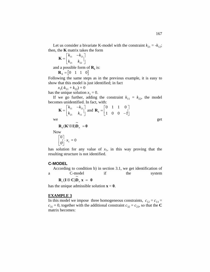
167
Let us consider a bivariate K-model with the constraint k21 = -k12; then, the K matrix takes the form
K =−⎡
⎣⎢
⎤
⎦⎥
k kk k
11 21
21 22
and a possible form of Rk is: R k = 0 1 1 0
Following the same steps as in the previous example, it is easy to show that this model is just identified; in fact x1(-k11 + k22) = 0 has the unique solution x1 = 0.
If we go further, adding the constraint k11 = k22, the model becomes unidentified. In fact, with:
K =−⎡
⎣⎢
⎤
⎦⎥
k kk k
11 21
21 11
and Rk = −⎡
⎣⎢⎤
⎦⎥0 1 1 01 0 0 1
we get R K I Dk n( ' )
~⊗ = 0
Now
00 1⎡
⎣⎢⎤
⎦⎥⋅ x = 0
has solution for any value of x1, in this way proving that the resulting structure is not identified.
C-MODEL
According to condition b) in section 3.1, we get identification of a C-model if the system R I C D x 0c n( )
~⊗ =
has the unique admissible solution x = 0. EXAMPLE 3 In this model we impose three homogeneous constraints, c12 = c13 = c31 = 0, together with the additional constraint c32 = c23, so that the C matrix becomes:

168
C =⎡
⎣
⎢⎢⎢
⎤
⎦
⎥⎥⎥
cc c c
c c
11
21 22 23
23 33
0 0
0
and a possible Rc matrix is
Rk = −
⎡
⎣
⎢⎢⎢⎢
⎤
⎦
⎥⎥⎥⎥
0 0 1 0 0 0 0 0 00 0 0 1 0 0 0 0 00 0 0 0 0 1 0 1 00 0 0 0 0 0 1 0 0
Simple calculations give the following system: Now we have to solve the system:
c c
c
c c c
c
x
x
x
23 33
11
21 33 22
11
1
2
3
0
0 0
0
0 0
−
+
−
⎡
⎣
⎢⎢⎢⎢⎢⎢
⎤
⎦
⎥⎥⎥⎥⎥⎥
⋅
⎡
⎣
⎢⎢⎢⎢
⎤
⎦
⎥⎥⎥⎥
( ) = 0
whose unique solution is given by x1 = x2 = x3 = 0. The model is identified, i.e. generally over-identified, the number
of constraints being greater than n (n-1)/2. EXAMPLE 4
Now, let us consider a model derived from a block diagonal structure. The C matrix takes the form:
C =⎡
⎣
⎢⎢⎢
⎤
⎦
⎥⎥⎥
c cc
c c
11 13
22
31 33
00 0
0
obtained imposing four homogeneous constraints: c12 = c21 = c23 = c32 = 0, so we can construct a Rc matrix with the following form:
R c =
⎡
⎣
⎢⎢⎢⎢⎢⎢
⎤
⎦
⎥⎥⎥⎥⎥⎥
0 1 0 0 0 0 0 0 0
0 0 0 1 0 0 0 0 0
0 0 0 0 0 1 0 0 0
0 0 0 0 0 0 0 1 0

169
Proceeding as usual we arrive at the system:
cc cc c
c
xxx
22
11 13
31 33
22
1
2
3
0 000
0 0
−−
−
⎡
⎣
⎢⎢⎢⎢
⎤
⎦
⎥⎥⎥⎥
⋅⎡
⎣
⎢⎢⎢
⎤
⎦
⎥⎥⎥
= 0
The second column of the coefficient matrix is equal to 0, so the system accepts any value for x2 as a solution. The model is unidentified and the non-identification rank is equal to 1 (i.e. the difference between the number of column and the actual rank of the 'identification matrix').
This example is connected to the BERNANKE.SRC procedure created by T. Doan for the RATS econometric package. In the introduction, the author mentions the concept of weak identification with respect to an AB-model where constraints of the same form as the ones we have just imposed hold, except for one parameter which, instead of being constrained to zero, has a free estimate close to zero.
The difficulties associated with the model, outlined by Doan, are due to the fact that in these cases we face a near block-diagonal structure, and the parameter close to zero is the one connecting two different blocks. In that case, the iterative estimation algorithm can easily fail to achieve convergence.
Following the approach described in this book, there seems to be no room for ambiguous concepts like weak identification of some parameters: the whole set of parameters are either identified or non-identified. In our view, the problem encountered by Doan is brought about by numerical difficulties in the estimation of a set of identified parameters. AB-MODEL
For the AB-model we follow the identification condition outlined in chapter 4, so our model is identified if the system:
R A BB z 0
R B BB D x z 0a
b
( n
( ' )
( ' ' )~
)
⊗ =
⊗ − =
⎧⎨⎪
⎩⎪
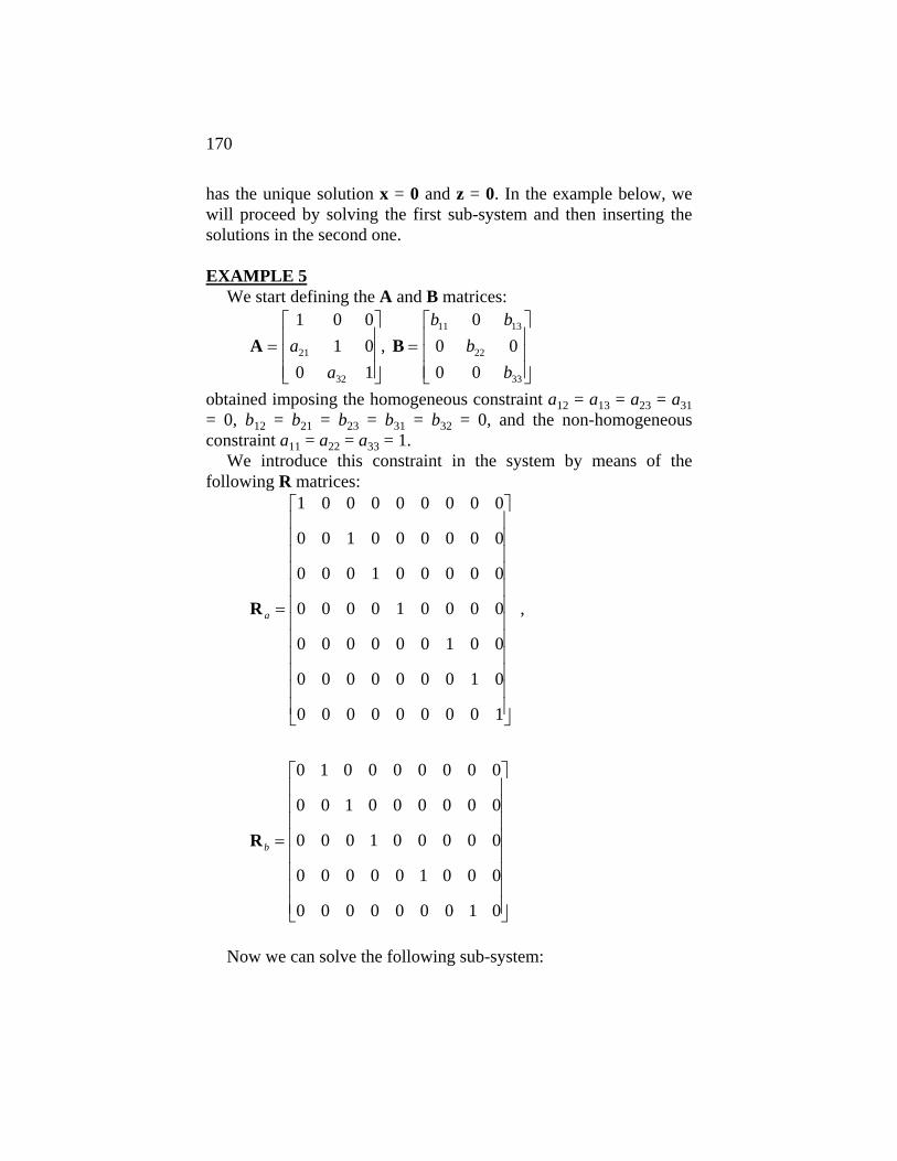
170
has the unique solution x = 0 and z = 0. In the example below, we will proceed by solving the first sub-system and then inserting the solutions in the second one. EXAMPLE 5
We start defining the A and B matrices:
A B=⎡
⎣
⎢⎢⎢
⎤
⎦
⎥⎥⎥
=⎡
⎣
⎢⎢⎢
⎤
⎦
⎥⎥⎥
1 0 01 0
0 1
00 00 0
21
32
11 13
22
33
aa
b bb
b,
obtained imposing the homogeneous constraint a12 = a13 = a23 = a31 = 0, b12 = b21 = b23 = b31 = b32 = 0, and the non-homogeneous constraint a11 = a22 = a33 = 1.
We introduce this constraint in the system by means of the following R matrices:
R
R
a
b
=
⎡
⎣
⎢⎢⎢⎢⎢⎢⎢⎢⎢⎢⎢⎢
⎤
⎦
⎥⎥⎥⎥⎥⎥⎥⎥⎥⎥⎥⎥
=
⎡
⎣
⎢⎢⎢⎢⎢⎢⎢⎢
⎤
⎦
⎥⎥⎥⎥⎥⎥⎥⎥
1 0 0 0 0 0 0 0 0
0 0 1 0 0 0 0 0 0
0 0 0 1 0 0 0 0 0
0 0 0 0 1 0 0 0 0
0 0 0 0 0 0 1 0 0
0 0 0 0 0 0 0 1 0
0 0 0 0 0 0 0 0 1
0 1 0 0 0 0 0 0 0
0 0 1 0 0 0 0 0 0
0 0 0 1 0 0 0 0 0
0 0 0 0 0 1 0 0 0
0 0 0 0 0 0 0 1 0
,
Now we can solve the following sub-system:

171
( )[ ]R A BB z 0a ⊗ =' where
( )[ ]R A B Ba ⊗ =' ( ) ( )( )( )[ ] ( ) ( ) ( )
( )( )[ ] ( ) ( ) ( )
( )( ) ( ) ( )
b b b b
b b b
a b b a b b b b b b
a b b
a b b a b b b b b b
a b b
a b b a b b b b
112
132
33 13
33 13 332
21 112
132
21 33 13 112
132
33 13
21 222
222
32 112
132
32 33 13 112
132
33 13
32 222
222
32 13 33 32 332
33 13 332
0 0 0 0 0 0 0
0 0 0 0 0 0 0
0 0 0 0 0
0 0 0 0 0 0 0
0 0 0 0 0
0 0 0 0 0 0 0
0 0 0 0 0
+
+ +
+ +
⎡
⎣
⎢⎢⎢⎢⎢⎢⎢⎢⎢⎢⎢⎢⎢
⎤
⎦
⎥⎥⎥⎥⎥⎥⎥⎥⎥⎥⎥⎥⎥
Substituting b11
2 +b132 = c and b33 b13 = d, we have to solve
[ ] ( )( )
[ ] ( )( )
( ) ( )
c d
d b
a c a d c d
a b b
a c a d c d
a b b
a b b a b d b
0 0 0 0 0 0 0
0 0 0 0 0 0 0
0 0 0 0 0
0 0 0 0 0 0 0
0 0 0 0 0
0 0 0 0 0 0 0
0 0 0 0 0
332
21 21
21 222
222
32 32
32 222
222
32 13 33 32 332
332
⎡
⎣
⎢⎢⎢⎢⎢⎢⎢⎢⎢⎢⎢⎢
⎤
⎦
⎥⎥⎥⎥⎥⎥⎥⎥⎥⎥⎥⎥
= z 0
which has the ∞2 solutions (z8 and z9 are parameters): z1 = 0
za a
z232 21
81
=
z3 = 0
z dc a
z432
9=
za
z532
81
= −

172
za
z632
91
= −
z dc
z7 8= −
z8 = z8 z9 = z9 Now we can insert the z vector in the second sub-system:
( )[ ]R B BB D x z 0b n⊗ −⎛⎝⎜
⎞⎠⎟ ='
~
where ( )[ ]R B BBb ⊗ ='
0 0 0 0 0 0 0 0
0 0 0 0 0 0 0
0 0 0 0 0 0 0
0 0 0 0 0 0 0
0 0 0 0 0 0 0
11 222
11 11 332
22 22
22 22 332
13 222
33 222
b b
b d b b
b c b d
b d b b
b b b b
⎡
⎣
⎢⎢⎢⎢⎢⎢⎢⎢
⎤
⎦
⎥⎥⎥⎥⎥⎥⎥⎥
and
~D x zn
zx zx zx z
zx zx zx z
z
− =
−−−
− −−−
− −− −−
⎡
⎣
⎢⎢⎢⎢⎢⎢⎢⎢⎢⎢⎢⎢
⎤
⎦
⎥⎥⎥⎥⎥⎥⎥⎥⎥⎥⎥⎥
1
1 2
2 3
1 4
5
3 6
2 7
3 8
9
so we have to solve the system: b11 b22
2 (x1-z2) = 0 (C.1) -z1 b11 d + b11 b33
2 (x2-z3) = 0 (C.2) b22 c (-x1-z4) +b22
d (x3-z6) = 0 (C.3)

173
b22 d (-x1-z4) +b22 b33
2 (x3-z6) = 0 (C.4) b13 b22
2 (x1-z2) +b33 b22
2 (-x3-z8) = 0 (C.5) Substituting to z1, ..., z7 their values with respect to z8 and z9,
obtained from the first sub-system, we get:
xa a
z132 21
81
= (C.1')
x2 = 0 (C.2') -c x1 + d x3 = 0 (C.3')
-d x1+ ba
dc a
z332
32
2
329−
⎛⎝⎜
⎞⎠⎟
+ b33
2 x3 = 0 (C.4')
x3 = -z8 (C.5') Now, let us focus our attention on equation (C.3') where:
d ca a
z z−⎛⎝⎜
⎞⎠⎟ = ⇒ =
32 218 80 0 (C.3'')
Now, looking at equation (C.4'), after some substitution we get:
ba
ba a
z33
32
13
32 219−
⎛⎝⎜
⎞⎠⎟
= 0 ⇒ z9 = 0 (C.4')
Inserting z8 = z9 = 0 in the first sub-system, we get z1 = z2 = ... = z7 = 0, so the system is identified.
In the same way we can get a generally over-identified model, simply adding -for example- the homogeneous constraint a32 = 0 so that the A matrix becomes:
A =⎡
⎣
⎢⎢⎢
⎤
⎦
⎥⎥⎥
1 0 01 0
0 0 121a
and a possible form for Ra is:

174
Ra =
⎡
⎣
⎢⎢⎢⎢⎢⎢⎢⎢⎢⎢
⎤
⎦
⎥⎥⎥⎥⎥⎥⎥⎥⎥⎥
1 0 0 0 0 0 0 0 00 0 1 0 0 0 0 0 00 0 0 1 0 0 0 0 00 0 0 0 1 0 0 0 00 0 0 0 0 1 0 0 00 0 0 0 0 0 1 0 00 0 0 0 0 0 0 1 00 0 0 0 0 0 0 0 1
Calculations for this example will not be included since they are very similar to those developed earlier.
174
REFERENCES
Amisano, G. (1995): Bayesian Inference on non Stationary Data, Ph.D. Thesis, Department of Economics, University of Warwick.
Amisano, G. (1996): Bayesian Inference in Cointegrated Systems, working paper, University of Brescia, Italy.
Amisano, G., M. Cesura, C. Giannini and M. Seghelini (1995): The Transmission Mechanism among Italian Interest Rates, working paper, University of Brescia, Italy.
Anderson, T. W. (1984): An Introduction to Multivariate Statistical Analysis, Wiley, New York.
Andrews, D.W.K. (1991): Heteroskedasticity and Autocorrelation Consistent Covariance Matrix Estimation, Econometrica, 59, 817-858.
Andrews, D.W.K., and J.C. Monahan (1992): An Improved Heteroskedasticity and Autocorrelation Consistent Covariance Matrix Estimation, Econometrica, 60, 953-966.
Baillie, R.T. (1987): Inference in Dynamic Models Containing 'Surprise' Variables, Journal of Econometrics, 35, 101-117.
Banerjee, A., J. Dolado, J.W. Galbraith and D.F. Hendry (1993): Co-Integration, Error Correction, and the Econometric Analysis of Non-Stationary Data, Oxford University Press, Oxford.
Banerjee, D.F. Hendry, and Smith, G.W. (1986): Exploring Equilibrium Relationships in Econometrics through Static Models: Some Monte Carlo Evidence, Oxford Bulletin of Economics and Statistics, 52, 95-104.
Bekker, P.A., and D.S.G. Pollock (1986): Identification of Linear Stochastic Models with Covariance Restrictions, Journal of Econometrics, 31, 179-208.
Berger, R.L, and D.F. Sinclair (1984): Testing Hypotheses Concerning Unions of Linear Subspaces, Journal of the American Statistical Association , 79, 158-163.
Bernanke, B. (1986): Alternative Explanations of the Money-Income Correlation, Carnegie-Rochester Conference Series on Public Policy, 25, 49-100.

175
Bernanke, B. and A. Blinder (1992): The Federal Funds Rate and the Channels of Money Transmission, American Economic Review, 82, 901-921.
Beveridge, S., and C.R. Nelson (1981): A New Approach to Decomposition of Economic Time Series into Permanent and Transitory Components, with Particular Attention to Measurement of the 'Business Cycle', Journal of Monetary Economics, 7, 151-174.
Blanchard, O.J. (1989): A Traditional Interpretation of Macro-economic Fluctuations, American Economic Review, 79, 1146-1164.
Blanchard, O.J, and D. Quah (1989): The Dynamic Effect of Aggregate Demand and Supply Disturbances, American Economic Review, 79, 655-673.
Blanchard, O.J, and D. Quah (1993): The Dynamic Effect of Aggregate Demand and Supply Disturbances: Reply, American Economic Review, 79, 653-658.
Blanchard, O.J, and M. W. Watson (1986): Are Business Cycles All Alike?, in R. Gordon (ed.): The American Business Cycle: Continuity and Change, NBER and University of Chicago Press.
Canova, F. (1991): The Sources of Financial Crisis: Pre- and Post-FED Evidence, International Economic Review, 32, 689-713.
Cappuccio, N. and D. Lubian (1995): A Comparison of Alternative Approaches to Estimation and Inference in Structural Long Run Economic Equilibria, mimeo, University of Padova, Italy.
Davidson, R. and J.G. Mac Kinnon (1994): Estimation and Inference in Econometrics, Oxford University Press, Oxford.
Dhrymes, P.J. (1978): Mathematics for Econometrics, Springer Verlag, New York.
Doan, T. (1992): RATS : User’s Manual. Version 4, ESTIMA. Doan, T., R.B. Litterman and C.Sims (1984): Forecasting and
Conditional Projections Using Realistic Prior Distributions, Econometric Reviews, 3, 1-100.
Engle, R. and C.W.J. Granger (1987): Co-integration and Error Correction: Estimation, Representation and Testing, Econometrica, 55, 251-276.

176
Geweke, J. (1984): Inference and Causality in Economic Time Series Models, in Z. Griliches and M.D. Intriligator (eds.): Handbook of Econometrics, Vol. II, North Holland, Amsterdam.
Giannini, C., A. Lanzarotti and M. Seghelini (1995): A Traditional Interpretation of Macroeconomic Fluctuations: the Case of Italy, European Journal of Political Economy, 11, 131-155.
Godfrey, L.G. (1988): Misspecification Tests in Econometrics, Cambridge University Press, Cambridge.
Granger, C.W.J (1969): Investigating Causal Relations by Econometric Models and Cross Spectral Methods, Econometrica, 37, 424-438.
Granger C.W.J. (1981): Some Properties of Time Series Data and Their Use in Econometric Model Specification, Journal of Econometrics, 16, 101-30.
Granger C.W.J., and P. Newbold (1974): Spurious Regressions in Econometrics, Journal of Econometrics, 2, 111-20.
Hall, P. (1994): Methodology and Theory for the Bootstrap, in R.F. Engle and D. L. McFadden (eds.): Handbook of Econometrics, Vol. 4, North-Holland, Amsterdam.
Hamilton (1994): Time Series Analysis, Princeton University Press. Hansen, H. and S. Johansen (1993): Recursive Estimation in
Cointegrated VAR Models, University of Copenhagen, Institute of Mathematical Statistics, pre-print 93-1.
Hansen, L.P and T.J. Sargent (1991): Rational Expectation Econometrics, Westview Press, Boulder and London.
Harvey, A.C. (1990): The Econometric Analysis of Time Series, LSE Handbooks of Economics, Philip Allan, London.
Hurwicz, L. (1962): On the Structural Form of Interdependent Systems, in Nagel, E., P Suppes, and A. Tarsky (eds.): Logic, Methodology and Philosophy of Science, Proceedings of the 1960 International Congress, Stanford University Press.
Johansen, S. (1988): Statistical Analysis of Cointegrating Vectors, Journal of Economic Dynamics and Control, 12, 231,-254.
Johansen, S. (1991) Estimation and Hypothesis Testing of Cointegrating Vectors in Gaussian Vector Autoregressive Models, Econometrica, 59, 1551-1580.

177
Johansen, S. (1992): Determination of the Cointegration Rank in the Presence of a Linear Trend, Oxford Bulletin of Economics and Statistics, 54, 383-97.
Johansen, S. (1995a): Likelihood Based Inference on Cointegration in the Vector Autoregressive Model, Oxford University Press, Oxford.
Johansen S. (1995b): Identifying Restrictions of Linear Equations: with Applications to Simultaneous Equations and Cointegration, Journal of Econometrics, 69, 111-132.
Johansen, S. and K. Juselius (1990): Maximum Likelihood Estimation and Inference on Cointegration - with applications to the demand for money, Oxford Bulletin of Economics and Statistics, 52, 2, 169-210.
Johansen, S. and K. Juselius (1994): Identification of the Long-Run and Short-Run Structure. An Application to the ISLM Model, Journal of Econometrics, 63, 7-36.
Keating, J.W. (1990): Identifying VAR Models Under Rational Expectations, Journal of Monetary Economics, 25, 453-476.
Killian, L. (1995): Small-Sample Confidence Intervals for Impulse Response Functions, working paper, Department of Economics, University of Pennsylvania.
King, R.G., C.I. Plosser, J.H. Stock and M. W. Watson (1991): Stochastic Trends and Economic Fluctuations, American Economic Review, 81, 819-840.
Kloek, T. and H.K. van Dijk (1978): Bayesian Estimates of Equation System Parameters: an Application of Integration by Monte Carlo, Econometrica, 46, 881-896.
Li, H. and G.S. Maddala (1996): Bootstrapping Time Series Models, Econometric Theory, 13(2), 115-195.
Lippi , M. and L. Reichlin (1993): The Dynamic Effects of Aggregate Demand and Supply Disturbances: Comment, American Economic Review, 83, 645-652.
Lippi, M. and L. Reichlin (1994): VAR Analysis, Non-Fundamental Representations Blaschke Matrices, Journal of Econometrics, 63, 307-325.
178
Litterman, R.B. (1979): Techniques of Forecasting Using Vector Autoregressions, Working paper # 115, Federal Reserve Bank of Minneapolis.
Litterman, R.B. (1986): Forecasting with Bayesian Vector Autoregression - Five Years of Experience, Journal of Business and Economic Statistics 4, 25-38.
Lütkepohl, H. (1989): A Note on the Asymptotic Distributions of the Impulse Response Functions of Estimated VAR models with Orthogonal Residuals, Journal of Econometrics, 42, 371-376.
Lütkepohl, H. (1990): Asymptotic Distribution of Impulse Response Functions and Forecasting Error Variance Decompositions of Vector Autoregressive Models, The Review of Economics and Statistics, 72, 116-125.
Lütkepohl, H (1991): Introduction to Multiple Time Series Analysis, Springer Verlag, New York
Lütkepohl, H. and H. E. Reimers (1992): Impulse Response Analysis of Cointegrated Systems with an Application to German Money Demand, Journal of Economic Dynamics and Control, 16, 53-78.
MacKinnon, J.G. (1983): Model Specification Tests against Non-Nested Alternatives, Econometric Reviews, 2, 85-157.
Magnus, J.R. (1988): Linear Structures, Griffin, London. Magnus, J.R., and H. Neudecker (1988): Matrix Differential
Calculus with Applications in Statistics and Econometrics, Wiley, New York.
Mosconi, R. (1996): MALCOLM (MAximum Likelihood Cointegration Analysis of Linear Models): The Theory and Practice of Cointegrating Analysis in RATS, forthcoming, Cafoscarina, Venice.
Nelson, C. and H. Kang (1981): Spurious Periodicity in Inappropriately Detrended Time Series, Econometrica, 49, 741-751.
Newey, W.K., and K.D. West (1987): A Simple, Positive Semi-Definite, Heteroskedasticity and Autocorrelation Consistent Covariance Matrix Estimator, Econometrica, 55, 703-708.

179
Nielsen, Bent (1995): Bartlett Correction of the Unit Root Test in Autoregressive Models, Nuffield College working paper.
Pagan, A. (1986): Two Stage and Related Estimators and Their Applications, Review of Economic Studies, LIII, 517-538.
Pantula, S.G. (1989): Testing for Unit Roots in Time Series Data, Econometric Theory, 5, 256-71.
Perron, P. and P.C.B. Phillips (1988): Testing for a Unit Root in Time Series Regression, Biometrika, 75, 335-348.
Pesaran, M. H. (1973): On the General Problem of Model Selection, Review of Economic Studies, 41, 153-171.
Phillips, P.C.B. (1983): Marginal Densities of Instrumental Variable Estimators in the General Single Equation Case, Advances in Econometrics, 2, 1-24.
Phillips, P.C.B. (1986): Understanding Spurious Regressions in Econometrics, Journal of Econometrics, 33, 311-40.
Phillips, P.C.B. (1991): Optimal Inference in Co-Integrated Systems, Econometrica, 62, 73-93
Phillips, P.C.B. (1994): Some exact Distribution Theory for Maximum Likelihood Estimators of Cointegrating Coefficients in Error Correction Models, Econometrica, 62, 73-93.
Phillips, P.C.B. and S.N. Durlauf (1986): Multiple Time Series Regression with Integrated Processes, Review of Economic Studies, 53, 473-95.
Phillips, P.C.B., and B.E. Hansen (1990): Statistical Inference in Instrumental Variables Regression with I(1) Processes, Review of Economic Studies, 57, 99-125.
Pollack, R.A., and T.J. Wales (1991): The Likelihood Dominance Criterion- A New Approach to Model Selection, Journal of Econometrics, 47, 227-242.
Pollock, D.S.G. (1979): The Algebra of Econometrics, Wiley, New York.
Quah, D. (1990): Permanent and Transitory Movements in Labor Income: An Explanation for 'Excess Smoothness' in Consumption, Journal of Political Economy, 98, 449-475.

180
Reimers, H. E. (1993): Lag order determination in cointegrated VAR systems with application to small German macro-models, paper presented to the ESEM congress 1993, Uppsala, Sweden.
Rothenberg T.J. (1971): Identification in Parametric Models, Econometrica, 39, 577-791.
Rothenberg T.J. (1973): Efficient Estimation with A-Priori Information, Yale University Press, New Haven.
Runkle, D.E. (1987): Vector Autoregressions and Reality, Journal of Business and Economic Statistics, 5, 437-442.
Sargan, J.D. (1988): Lectures on Advanced Econometric Theory, Oxford, Basil Blackwell.
Schmidt P. and P.C.B. Phillips (1992): Testing for a Unit Root in the Presence of Deterministic Trends, Oxford Bulletin of Economics and Statistics, 54, 257-287.
Serfling, R.F. (1980): Approximation Theorems of Mathematical Statistics, Wiley, New York.
Shapiro, M. and M.W. Watson (1988): Sources of Business Cycle Fluctuations, NBER Macroeconomic Annual, MIT press, 3, 111-156.
Sims C.A. (1972): Money, Income and Causality, American Economic Review, 62, 540-552.
Sims, C.A. (1980): Macroeconomics and reality, Econometrica, 48, 1-48
Sims ,C.A.(1982): Policy Analysis with Econometric Models, Brookings Papers on Economic Activity, 2, 107-152.
Sims, C.A.(1986): Are Forecasting Models Usable for Policy Analysis?, Quarterly Review of the Federal Reserve Bank of Minneapolis, winter, 2-16.
Sims C.A. (1988), Identifying Policy Effects, in Bryant et al. (eds.): Empirical Macroeconomics for Interdependent Economies, Brooking Institution, 305-321.
Sims C.A. ,and T. Zha (1995), Error Bands for Impulse Responses, working paper, University of Yale.

181
Stock, J.H. (1987): Asymptotic Properties of Least Squares Estimators of Co-Integrating Vectors, Econometrica, 55, 1035-56.
Stock, J.H., and M. W. Watson (1988): Testing for Common Trends, Journal of the American Statistical Association, 83, 1097-1107.
Taylor, J. B. (1986): Aggregate Dynamics and Staggered Contracts, Journal of Political Economy, 88, 1-24.
Theil, H. and A.S. Goldberger (1961): On pure and mixed statistical estimation in economics, International Economic Review, 2, 65-78.
Wegge, L. (1965): Identifiability Criteria for a System of Equations as a Whole, Australian Journal of Statistics, 7, 67-77.
White, H. (1982): Maximum Likelihood Estimation of Misspecified Models, Econometrica, 50, 1-26.
White, H. (1983): Estimation, Inference and Specification Analysis, Discussion paper # 83-26, University of California at San Diego.
White, H. (1984): Asymptotic Theory for Econometricians, Academic Press, Orlando.
Wiener, N. (1956): The Theory of Prediction, in E.F. Beckenback (ed.): Modern Mathematics for Engineers.
Yule, G.U. (1926): Why Do We Sometimes Get Nonsense Correlations Between Time Series? A Study in Sampling and the Nature of Time Series, Journal of the Royal Statistical Society, 89, 1-64.
Zellner, A. (1971): An introduction to Bayesian Inference in Econometrics, Wiley, New York


