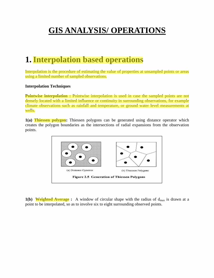
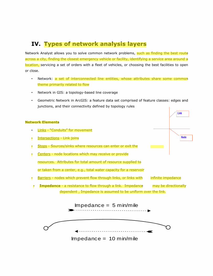
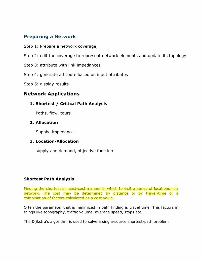
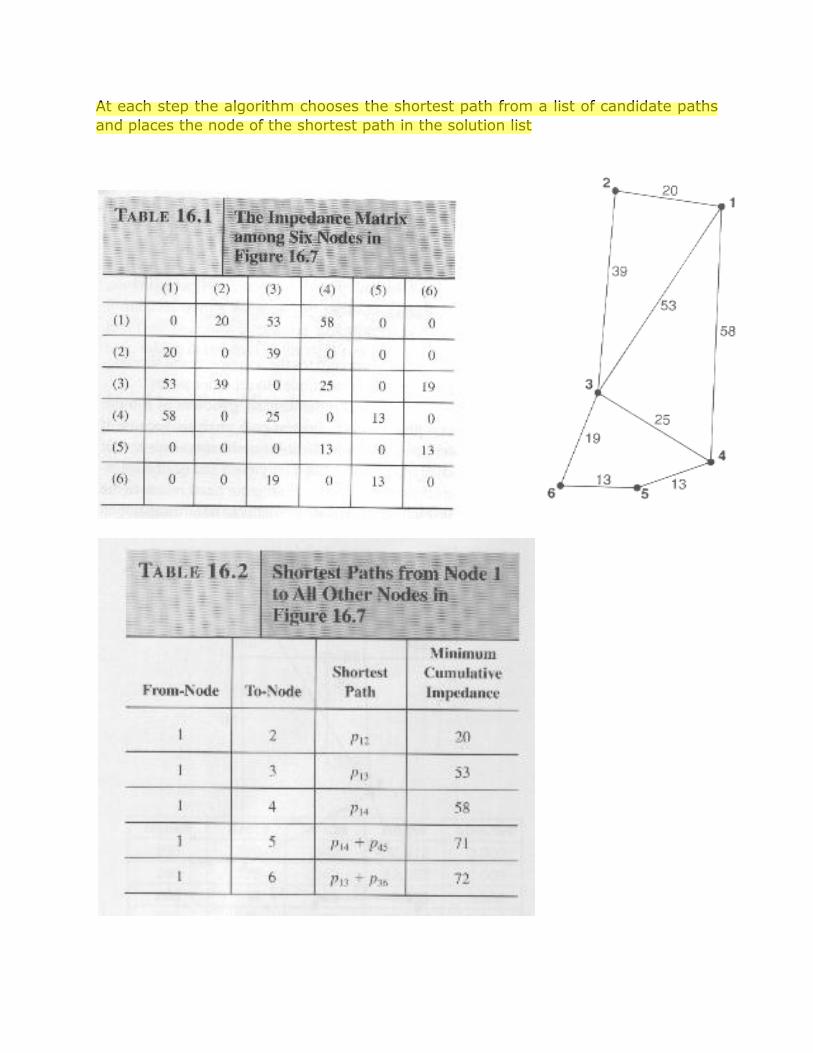
GIS ANALYSIS/ OPERATIONS 1. Interpolation based operations Interpolation is the procedure of estimating the value of properties at unsampled points or areas using a limited number of sampled observations. Interpolation Techniques Pointwise interpolation : Pointwise interpolation is used in case the sampled points are not densely located with a limited influence or continuity in surrounding observations, for example climate observations such as rainfall and temperature, or ground water level measurements at wells. 1(a) Thiessen polygon: Thiessen polygons can be generated using distance operator which creates the polygon boundaries as the intersections of radial expansions from the observation points. 1(b) Weighted Average : A window of circular shape with the radius of d max is drawn at a point to be interpolated, so as to involve six to eight surrounding observed points.
Transcript
GIS ANALYSIS/ OPERATIONS
1. Interpolation based operations
Interpolation is the procedure of estimating the value of properties at unsampled points or areas
using a limited number of sampled observations.
Interpolation Techniques
Pointwise interpolation : Pointwise interpolation is used in case the sampled points are not
densely located with a limited influence or continuity in surrounding observations, for example
climate observations such as rainfall and temperature, or ground water level measurements at
wells.
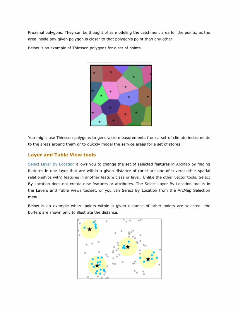
1(a) Thiessen polygon: Thiessen polygons can be generated using distance operator which
creates the polygon boundaries as the intersections of radial expansions from the observation
points.
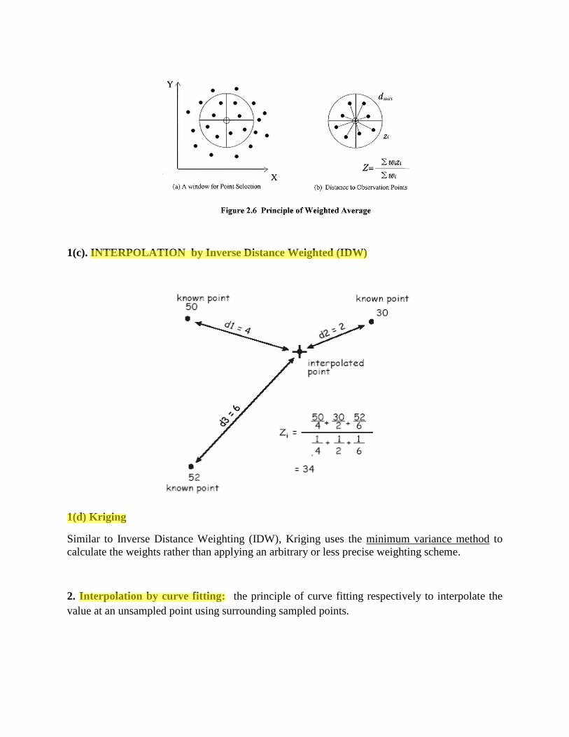
1(b) Weighted Average : A window of circular shape with the radius of dmax is drawn at a
point to be interpolated, so as to involve six to eight surrounding observed points.
hp
Highlight
hp
Highlight
hp
Highlight
hp
Highlight
hp
Highlight
1(c). INTERPOLATION by Inverse Distance Weighted (IDW)
1(d) Kriging
Similar to Inverse Distance Weighting (IDW), Kriging uses the minimum variance method to
calculate the weights rather than applying an arbitrary or less precise weighting scheme.
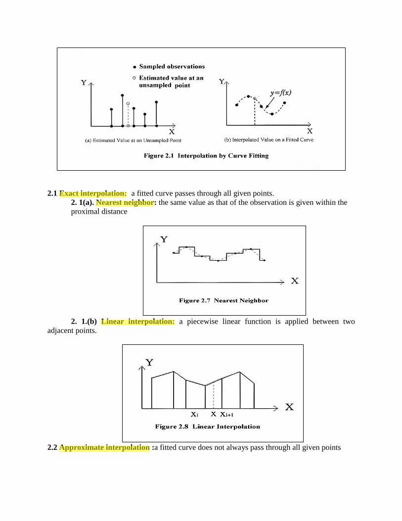
2. Interpolation by curve fitting: the principle of curve fitting respectively to interpolate the
value at an unsampled point using surrounding sampled points.
hp
Highlight
hp
Highlight
hp
Highlight
2.1 Exact interpolation: a fitted curve passes through all given points.
2. 1(a). Nearest neighbor: the same value as that of the observation is given within the
proximal distance
2. 1.(b) Linear interpolation: a piecewise linear function is applied between two
adjacent points.
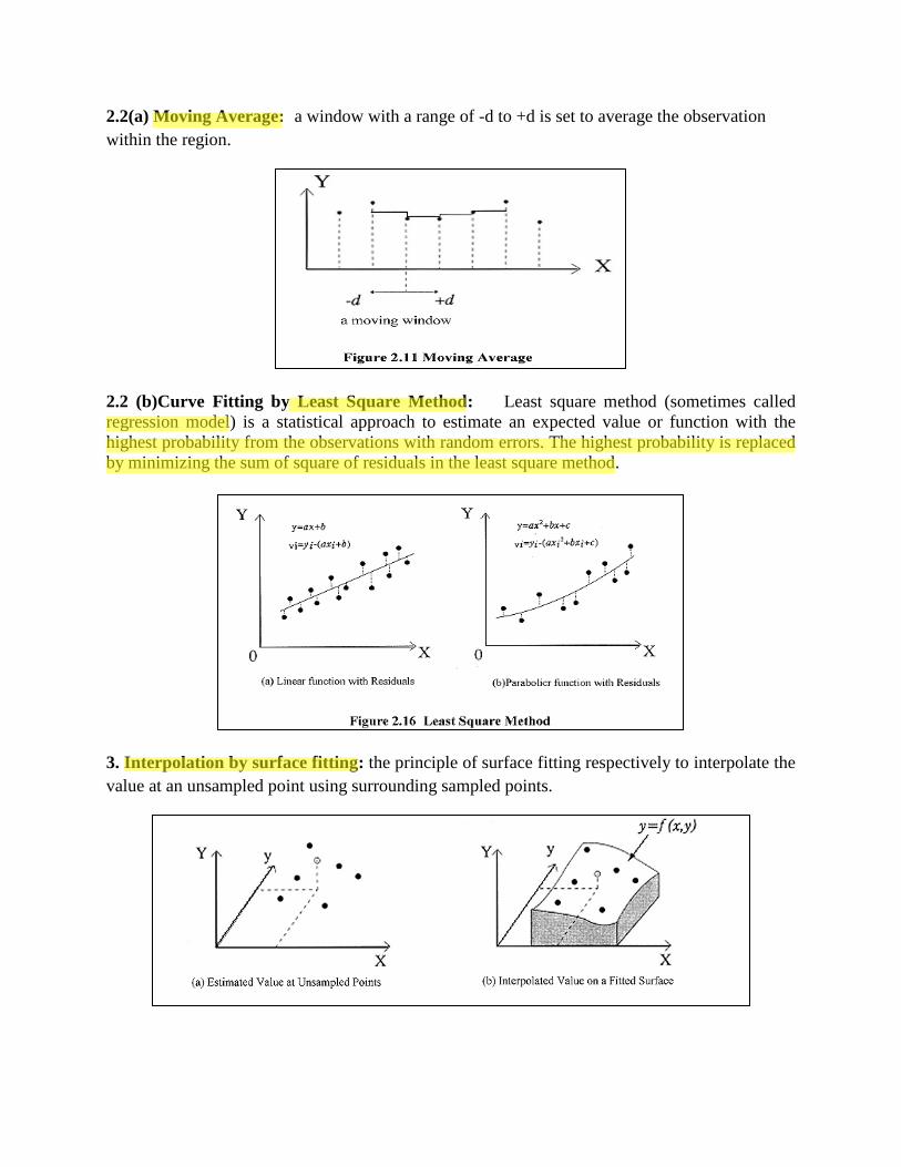
2.2 Approximate interpolation :a fitted curve does not always pass through all given points
hp
Highlight
hp
Highlight
hp
Highlight
hp
Highlight
2.2(a) Moving Average: a window with a range of -d to +d is set to average the observation
within the region.
2.2 (b)Curve Fitting by Least Square Method: Least square method (sometimes called
regression model) is a statistical approach to estimate an expected value or function with the
highest probability from the observations with random errors. The highest probability is replaced
by minimizing the sum of square of residuals in the least square method.
3. Interpolation by surface fitting: the principle of surface fitting respectively to interpolate the
value at an unsampled point using surrounding sampled points.
hp
Highlight
hp
Highlight
hp
Highlight
hp
Highlight
hp
Highlight
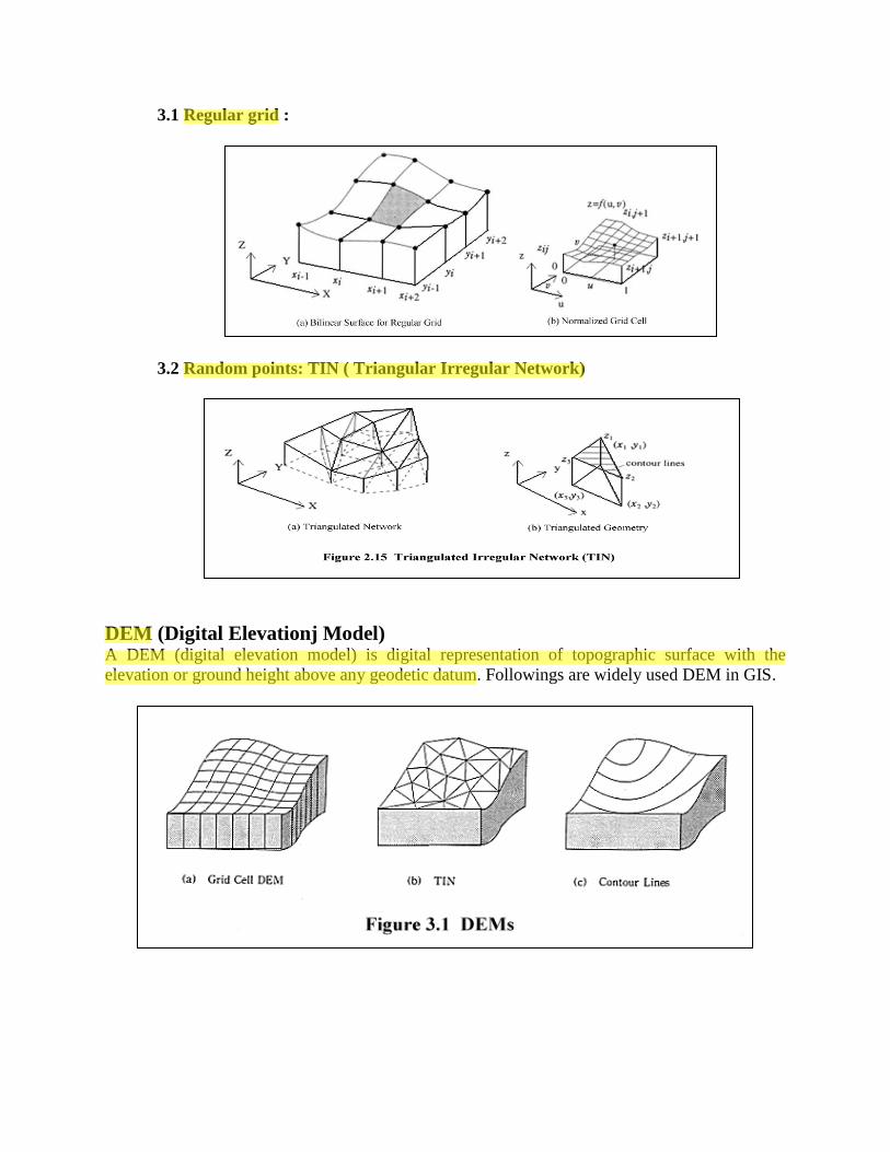
3.1 Regular grid :
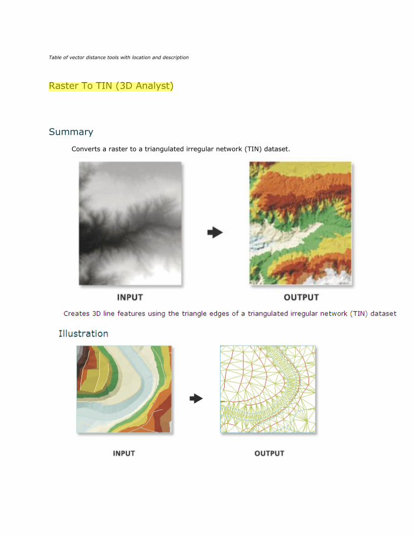
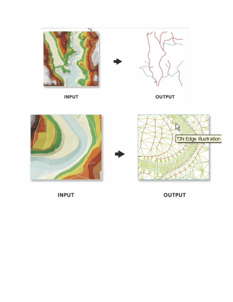
3.2 Random points: TIN ( Triangular Irregular Network)
DEM (Digital Elevationj Model) A DEM (digital elevation model) is digital representation of topographic surface with the
elevation or ground height above any geodetic datum. Followings are widely used DEM in GIS.
hp
Highlight
hp
Highlight
hp
Highlight
1.1 Density Analysis
Density analysis takes known quantities of some phenomenon and spreads them across the
landscape based on the quantity that is measured at each location and the spatial relationship of
the locations of the measured quantities.
Why map density?
Density surfaces show where point or line features are concentrated. For example, you might
have a point value for each town representing the total number of people in the town, but you
want to learn more about the spread of population over the region. Since all the people in each
town do not live at the population point, by calculating density, you can create a surface showing
the predicted distribution of the population throughout the landscape.
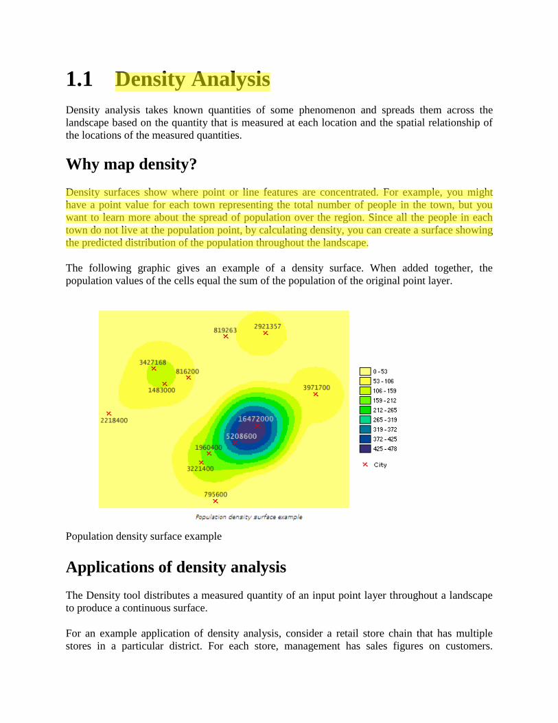
The following graphic gives an example of a density surface. When added together, the
population values of the cells equal the sum of the population of the original point layer.
Population density surface example
Applications of density analysis
The Density tool distributes a measured quantity of an input point layer throughout a landscape
to produce a continuous surface.
For an example application of density analysis, consider a retail store chain that has multiple
stores in a particular district. For each store, management has sales figures on customers.
hp
Highlight
Proximity analysis
hp
Highlight
Management assumes that customers patronize one store over another based on how far they
have to travel. In this example, it is natural to assume that any single customer will always
choose the closest store. The farther away from the closest store, the farther the customer will
need to travel to that store. But shoppers farther away may also shop at other stores. Management
wants to study the distribution of where the customers live. From the sales figures and the spatial
distribution of the stores, management wants to create a surface of customers by intelligently
spreading the customers out across the landscape.
To accomplish this task, the Density tool considers where each store is in relation to other stores,
the quantity of customers shopping at each store, and how many cells need to share a portion of
the measured quantity (the shoppers). The cells nearer the measured points, the stores, receive
higher proportions of the measured quantity than those farther away.
II. Understanding overlay analysis
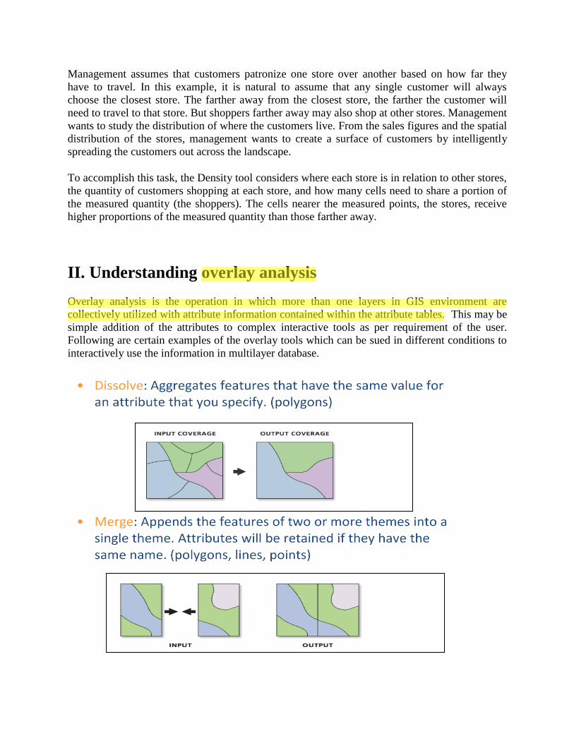
Overlay analysis is the operation in which more than one layers in GIS environment are
collectively utilized with attribute information contained within the attribute tables. This may be
simple addition of the attributes to complex interactive tools as per requirement of the user.
Following are certain examples of the overlay tools which can be sued in different conditions to
interactively use the information in multilayer database.
hp
Highlight
hp
Highlight
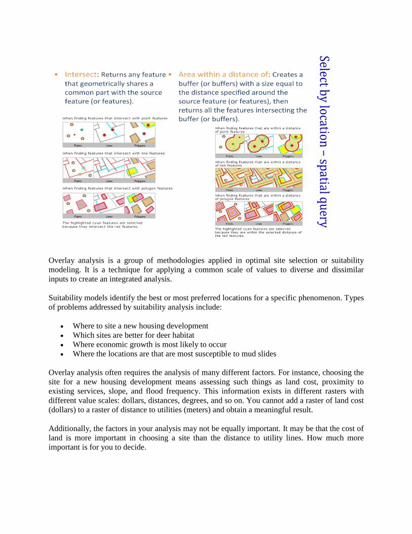
Overlay analysis is a group of methodologies applied in optimal site selection or suitability
modeling. It is a technique for applying a common scale of values to diverse and dissimilar
inputs to create an integrated analysis.
Suitability models identify the best or most preferred locations for a specific phenomenon. Types
of problems addressed by suitability analysis include:
Where to site a new housing development
Which sites are better for deer habitat
Where economic growth is most likely to occur
Where the locations are that are most susceptible to mud slides
Overlay analysis often requires the analysis of many different factors. For instance, choosing the
site for a new housing development means assessing such things as land cost, proximity to
existing services, slope, and flood frequency. This information exists in different rasters with
different value scales: dollars, distances, degrees, and so on. You cannot add a raster of land cost
(dollars) to a raster of distance to utilities (meters) and obtain a meaningful result.
Additionally, the factors in your analysis may not be equally important. It may be that the cost of
land is more important in choosing a site than the distance to utility lines. How much more
important is for you to decide.
Even within a single raster, you must prioritize values. Some values in a particular raster may be
ideal for your purposes (for example, slopes of 0 to 5 degrees), while others may be good, others
bad, and still others unacceptable.
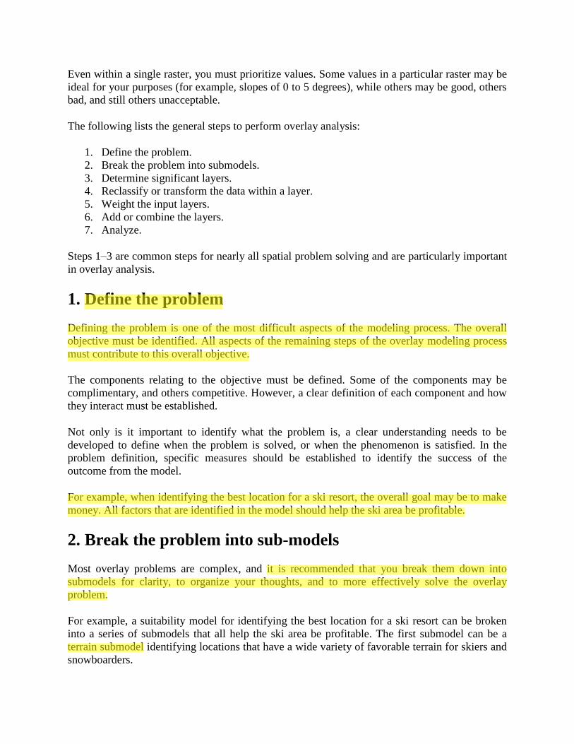
The following lists the general steps to perform overlay analysis:
1. Define the problem.
2. Break the problem into submodels.
3. Determine significant layers.
4. Reclassify or transform the data within a layer.
5. Weight the input layers.
6. Add or combine the layers.
7. Analyze.
Steps 1–3 are common steps for nearly all spatial problem solving and are particularly important
in overlay analysis.
1. Define the problem
Defining the problem is one of the most difficult aspects of the modeling process. The overall
objective must be identified. All aspects of the remaining steps of the overlay modeling process
must contribute to this overall objective.
The components relating to the objective must be defined. Some of the components may be
complimentary, and others competitive. However, a clear definition of each component and how
they interact must be established.
Not only is it important to identify what the problem is, a clear understanding needs to be
developed to define when the problem is solved, or when the phenomenon is satisfied. In the
problem definition, specific measures should be established to identify the success of the
outcome from the model.
For example, when identifying the best location for a ski resort, the overall goal may be to make
money. All factors that are identified in the model should help the ski area be profitable.
2. Break the problem into sub-models
Most overlay problems are complex, and it is recommended that you break them down into
submodels for clarity, to organize your thoughts, and to more effectively solve the overlay
problem.
For example, a suitability model for identifying the best location for a ski resort can be broken
into a series of submodels that all help the ski area be profitable. The first submodel can be a
terrain submodel identifying locations that have a wide variety of favorable terrain for skiers and
snowboarders.
hp
Highlight
hp
Highlight
hp
Highlight
hp
Highlight
hp
Highlight
3. Determine significant layers
The attributes or layers that affect each submodel need to be identified. Each factor captures and
describes a component of the phenomena the submodel is defining. Each factor contributes to the
goals of the submodel, and each submodel contributes to the overall goal of the overlay model.
All and only factors that contribute to defining the phenomenon should be included in the
overlay model.
For certain factors, the layers may need to be created. For example, it may be more desirable to
be closer to a major road. To identify the distance each cell is from a road, Euclidean Distance
may be run to create the distance raster.
Because of the potential different ranges of values and the different types of numbering systems
each input layer may have, before the multiple factors can be combined for analysis, each must
be reclassified or transformed to a common ratio scale.
Common scales can be predetermined, such as a 1 to 9 or a 1 to 10 scale, with the higher value
being more favorable, or the scale can be on a 0 to 1 scale, defining the possibility of belonging
to a specific set.
4. Weight
Certain factors may be more important to the overall goal than others. If this is the case, before
the factors are combined, the factors can be weighted based on their importance. For example, in
the building submodel for siting the ski resort, the slope criteria may be twice as important to the
cost of construction as the distance from a road. Therefore, before combining the two layers, the
slope criteria should be multiplied twice as much as distance to roads.
6. Add/Combine
In overlay analysis, it is desirable to establish the relationship of all the input factors together to
identify the desirable locations that meet the goals of the model. For example, the input layers,
once weighted appropriately, can be added together in an additive weighted overlay model. In
this combination approach, it is assumed that the more favorable the factors, the more desirable
the location will be. Thus, the higher the value on the resulting output raster, the more desirable
the location will be.
Other combining approaches can be applied. For example, in a fuzzy logic overlay analysis, the
combination approaches explore the possibility of membership of a location to multiple sets.
7. Analyze
hp
Highlight
hp
Highlight
hp
Highlight
hp
Highlight
hp
Highlight
hp
Highlight
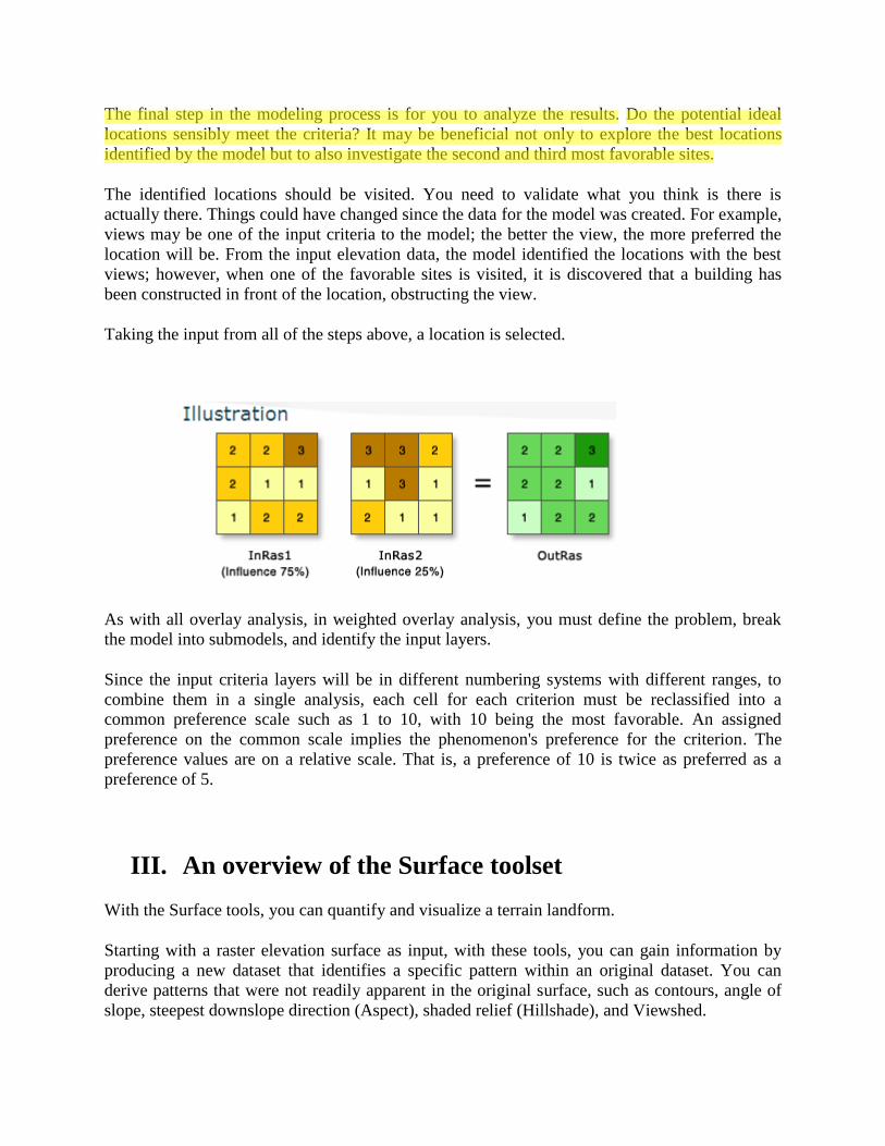
The final step in the modeling process is for you to analyze the results. Do the potential ideal
locations sensibly meet the criteria? It may be beneficial not only to explore the best locations
identified by the model but to also investigate the second and third most favorable sites.
The identified locations should be visited. You need to validate what you think is there is
actually there. Things could have changed since the data for the model was created. For example,
views may be one of the input criteria to the model; the better the view, the more preferred the
location will be. From the input elevation data, the model identified the locations with the best
views; however, when one of the favorable sites is visited, it is discovered that a building has
been constructed in front of the location, obstructing the view.
Taking the input from all of the steps above, a location is selected.
As with all overlay analysis, in weighted overlay analysis, you must define the problem, break
the model into submodels, and identify the input layers.
Since the input criteria layers will be in different numbering systems with different ranges, to
combine them in a single analysis, each cell for each criterion must be reclassified into a
common preference scale such as 1 to 10, with 10 being the most favorable. An assigned
preference on the common scale implies the phenomenon's preference for the criterion. The
preference values are on a relative scale. That is, a preference of 10 is twice as preferred as a
preference of 5.
III. An overview of the Surface toolset
With the Surface tools, you can quantify and visualize a terrain landform.
Starting with a raster elevation surface as input, with these tools, you can gain information by
producing a new dataset that identifies a specific pattern within an original dataset. You can
derive patterns that were not readily apparent in the original surface, such as contours, angle of
slope, steepest downslope direction (Aspect), shaded relief (Hillshade), and Viewshed.
hp
Highlight
hp
Highlight
hp
Highlight
Each surface tool provides insight into a surface that can be used as an end in itself or as input
into additional analysis.
Tool Description
Aspect
Derives aspect from a raster surface. The aspect identifies the downslope
direction of the maximum rate of change in value from each cell to its neighbors.
Contour Creates a line feature class of contours (isolines) from a raster surface.
Contour List Creates a feature class of selected contour values from a raster surface.
Contour with
Barriers
Creates contours from a raster surface. The inclusion of barrier features will
allow one to independently generate contours on either side of a barrier.
Curvature Calculates the curvature of a raster surface, optionally including profile and plan
curvature.
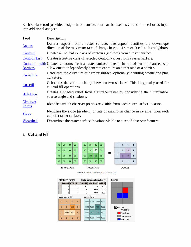
Cut Fill
Calculates the volume change between two surfaces. This is typically used for
cut and fill operations.
Hillshade
Creates a shaded relief from a surface raster by considering the illumination
source angle and shadows.
Observer
Points
Identifies which observer points are visible from each raster surface location.
Slope
Identifies the slope (gradient, or rate of maximum change in z-value) from each
cell of a raster surface.
Viewshed Determines the raster surface locations visible to a set of observer features.