GIS measured environmental correlates of activeschool transport: A systematic review of14 studiesBonny Yee-Man Wong1*, Guy Faulkner1 and Ron Buliung2
Abstract
Background: Emerging frameworks to examine active school transportation (AST) commonly emphasize the builtenvironment (BE) as having an influence on travel mode decisions. Objective measures of BE attributes have beenrecommended for advancing knowledge about the influence of the BE on school travel mode choice. An updatedsystematic review on the relationships between GIS-measured BE attributes and AST is required to inform futureresearch in this area. The objectives of this review are: i) to examine and summarize the relationships betweenobjectively measured BE features and AST in children and adolescents and ii) to critically discuss GISmethodologies used in this context.
Methods: Six electronic databases, and websites were systematically searched, and reference lists were searchedand screened to identify studies examining AST in students aged five to 18 and reporting GIS as an environmentalmeasurement tool. Fourteen cross-sectional studies were identified. The analyses were classified in terms of density,diversity, and design and further differentiated by the measures used or environmental condition examined.
Results: Only distance was consistently found to be negatively associated with AST. Consistent findings of positiveor negative associations were not found for land use mix, residential density, and intersection density. Potentialmodifiers of any relationship between these attributes and AST included age, school travel mode, route direction(e.g., to/from school), and trip-end (home or school). Methodological limitations included inconsistencies ingeocoding, selection of study sites, buffer methods and the shape of zones (Modifiable Areal Unit Problem[MAUP]), the quality of road and pedestrian infrastructure data, and school route estimation.
Conclusions: The inconsistent use of spatial concepts limits the ability to draw conclusions about the relationshipbetween objectively measured environmental attributes and AST. Future research should explore standardizingbuffer size, assess the quality of street network datasets and, if necessary, customize existing datasets, and explorefurther attributes linked to safety.
BackgroundIn the context of increasing prevalence of obesity andoverweight in children and youth [1], the considerationof active school transport (AST) as an important andutilitarian source of physical activity is of interest. Chil-dren who walk to school are more physically active thanchildren who are driven [2]. However, there has been aconsistent decline in the use of active modes (i.e., walk-ing, biking) to and from school observed in Western
nations [3]. For example, in the Greater Toronto Area,Canada’s largest city-region, walking mode share fortrips to school declined between 1986 and 2001 (53%-42% for 11-13 year olds, 39%-31% for 14-15 year olds)[4] while car trips have increased. The immersion ofchildren into the culture of automobility, through paren-tal/caregiver decisions regarding mode choice for dailyactivities, could establish both short and long-term(through adolescence and into adulthood) expectationsregarding mobility that place the automobile at the cen-tre of everyday life. As lifelong patterns of physical activ-ity are established in childhood [5], encouraging andenabling active transportation for daily activities at a
* Correspondence: [email protected] of Physical Education & Health, University of TorontoFull list of author information is available at the end of the article
Wong et al. International Journal of Behavioral Nutrition and Physical Activity 2011, 8:39http://www.ijbnpa.org/content/8/1/39
young age may be beneficial over the long-term in termsof meeting urban planning and public health goalsoriented toward the production of active, healthy, andsustainable lifestyles.A wide range of correlates of active travel to and from
school have been studied including demographic, indivi-dual, family, school, social and physical environmentalfactors [3]. McMillan [6] developed one conceptual fra-mework to examine children’s school transportationbehaviour that incorporates these commonly examinedfactors. In her framework, parents are assumed to makethe ultimate decision about whether their child can walkto school. This decision is indirectly related to ‘urbanform’. That is, aspects of urban form are processed byparents and their perceptions, beliefs and attitudes (e.g.,regarding traffic or neighbourhood safety) mediate theirdecisions about their child’s school travel. Socio-demo-graphic variables, such as socioeconomic status, mayalso interact with these perceptions to influence parents’final decisions about school transport mode.Given the conceptualized importance of the environ-
ment in the context of AST in McMillan’s [6] and otherframeworks (e.g., Panter et al. [7]), objective measure-ment of the separate but related dimensions of urbanform - i.e., the organization and physical form of landuse and transportation (systems and services) is crucialto moving from a conceptual to an empirical under-standing of school travel behaviour. Existing studies onphysical activity, however, have largely relied on self-report measures of the environment [8].This may beappropriate if it is how the elements of the environmentare perceived by parents that is critical to the beha-vioural outcome [3]. However, physically active partici-pants may be more aware of how their neighbourhoodfacilitates physical activity than inactive ones (e.g., walk-ers may know better the location of streets with side-walks than those who do not walk as often). Therefore,active and inactive research participants located withinthe same neighbourhood may indeed have very differentperceptions about the environment they live in. Hence,measuring aspects of the built environment subjectively(e.g., through self-report) may not accurately assess theeffect of the actual BE on AST. Accordingly, objectivemeasurement of the built environment, informed by anunderstanding of how the built environment is con-structed (with regard to policy and planning), derivedfrom Geographic Information Systems (GIS) - enabledanalyses of digital representations/models of the landuse and transportation elements of the built environ-ment, is a necessary complement to self-report and/orqualitative assessment.The built environment may influence travel demand
across three general dimensions–density, diversity, anddesign, the so-called 3Ds [9], and these qualities may be
measured around the home, school, or routes to andfrom school [10]. Regarding density, compact neigh-bourhoods may encourage non-motorised travel andreduce single occupant vehicle (SOV) travel by bringingorigins and destinations closer together. Moreover, com-pact neighbourhoods could increase non-motorised tra-vel in other ways such as having greater land use mix,less parking, and improved transit level of service. Dis-tance can be considered as an operational measure ofthe concept of ‘density.’ For example, a higher density ofschools within a city should produce shorter schooltrips, on average, than a more sparsely populated geo-graphical distribution of schools. Similarly, land usediversity, characterized by having a mix of destinationspotentially makes it more convenient to develop tripchains across a set of activities using active modes suchas walking or biking. Design features, including thestreet pattern (e.g., gridded street patterns have greaterconnectivity), and pedestrian and cyclist infrastructure,may increase the accessibility of different destinations bynon-motorized travel. In addition, design features suchas streets with shaded trees can represent an aestheticthat may be appealing to those considering the use ofnon-motorized modes for short trips.This 3Ds framework was originally applied to the con-
text of adult travel behaviour but it can be usefullyextended as a framework for exploring children’s schooltransport and organizing existing literature on the sub-ject. Several systematic reviews [3,7,8,11] have examinedthe impact of the built environment on children’s ASTor active transport. For example, short distances [8],having walking or cycling paths [7,8], few hills [11], androute directness [11] have been found to be positivelyassociated with AST. These findings are primarily basedon self-report. Pont and colleagues’ recent systematicreview [8] only included 4 studies which measuredurban form objectively. Additionally, existing systematicreviews do not explicitly analyse how the built environ-ment was being measured using GIS. Given increasinginterest in how the built environment may influenceAST, a more detailed systematic review is required toinform research and practice regarding what we cur-rently know about the relationship between objectivelymeasured aspects of the built environment and AST;and to identify methodological implications for research-ers interested in examining this relationship.
MethodsSearching strategies and databases searchedThis review consisted of a search of published literaturein the English language. Databases were searched usingkeywords contained in the title, abstract, MESH head-ings, or descriptor terms. The search strategies involvedthree stages: 1) a combination of keywords on active
Wong et al. International Journal of Behavioral Nutrition and Physical Activity 2011, 8:39http://www.ijbnpa.org/content/8/1/39
Page 2 of 22
school transport (active school transport, active com-muting to (from) school, walking to (from) school, (bi)cycling to (from) school, biking to (from) school, walkto (from) school, cycle to (from) school, mode choice to(from) school, commuting to (from) school, commute to(from) school, child pedestrian, child cyclist, safe routeto school, mode to (from) school, travel to (from)school), keywords on the BE (physical environment,urban planning, neighbourhood, BE, walkability, roadsafety, crime, aesthetic, transportation, traffic, urbandesign, connectivity, distance, sprawl, socio-economic,trail, open space, greenway) and keywords of GIS (Geo-graphic Information Systems, Geographical InformationSystems, GIS); 2) a combination of keywords on activeschool transport and keywords on the BE; and 3) key-words on active school transport. Databases that weresearched included Web of Science (1960 - May 2010),Geobase (1973-May 2010), Scopus (1960-May 2010),Medline (1950 to May week 3 2010), Transport (1960-May 2010) and Sport Discus (1960-May 2010). Previousreviews were also examined. References within identifiedarticles were reviewed for further studies.
Inclusion/exclusion criteriaEach included study had to have: 1) participantsbetween 5 and 18 years of age (elementary or high
school students) as the study sample; 2) GIS as a mea-surement and/or analysis tool; 3) at least one variablerelated to the built environment relevant to activeschool transport as an independent variable; 4) at leastone variable related to school transport as a dependentvariable; 5) and reported empirical data on the builtenvironment and school transport.
Systematic review processFigure 1 shows the search and retrieval process. Thenumbers of references searched from each databasewere 2963 (Web of Science), 389 (Geobase), 1920 (Sco-pus), 373 (Medline), 835 (Transport), and 386 (SportDiscus). After reviewing each strategy and removingduplicates, 5610 references were found of which 63were identified following the screening of titles andabstracts. Four were conference papers and not availableand hence were excluded. Full texts of 59 publicationswere retrieved. Six reviews were excluded; their refer-ence lists were reviewed and potential articles wereidentified. Thirty-six did not measure the built environ-ment with GIS. Another three examined general activetransport among children and/or adolescents and wereexcluded. Two studies were excluded - one was a casestudy that did not provide statistical data regarding rele-vant travel mode and built environment relationships
5610 non-duplicated
2963 Web of science 389 Geobase 1920 Scopus 835 Transport 386 Sport Discus
63 identified
59 retrieved full-text
12 INCLUDED
16 identified and retrieved full-text
2 INCLUDED
4 conference papers excluded
Eligibility criteria screening
Screening reference lists
Eligibility criteria screening
Total 14 INCLUDED
Screening reference lists
6 Systematic reviews identified from full-text retrieval
373 Medline
Figure 1 The flow chart of systematic review process.
Wong et al. International Journal of Behavioral Nutrition and Physical Activity 2011, 8:39http://www.ijbnpa.org/content/8/1/39
Page 3 of 22
[12] and the second study used GIS techniques to esti-mate the number of school age children in Georgia liv-ing within a safe and reasonable walking distance fromschool [13]. Twelve publications were included at thisstage. From reference lists of identified articles and sys-tematic reviews [3,6-8,11,14,15], 16 additional potentialpublications were identified and their full-texts wereretrieved, of which eight did not examine AST, threedid not measure the built environment, another two didnot measure the built environment with GIS, and onestudied general active transport. Ultimately, 14 pub-lished studies were included in this review.
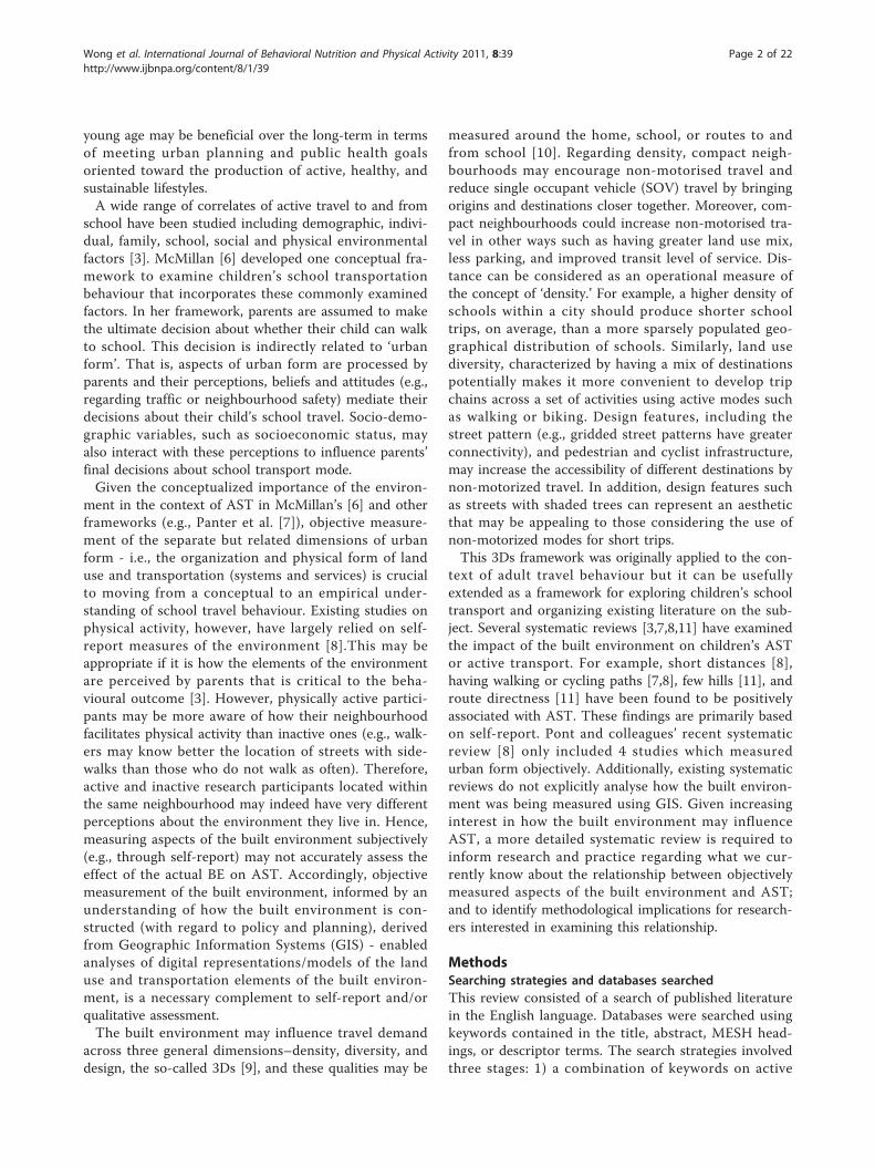
ResultsAll reviewed studies were cross-sectional (Table 1), mostwere American [16-22], three were Canadian [23-25],two European [26,27], one Australian [28], and one Tai-wanese [29]. Five studies [16,18,19,22,26] included bothchildren and adolescents. Seven studies included chil-dren only [20,23-25,27-29] and two included adolescentsonly [17,21]. For the purpose of description, elements ofthe built environment examined in these studies havebeen organized using the 3Ds framework described ear-lier [9].
DensitySix studies measured residential density as either thenumber of residential units or the total number of resi-dents divided by the area of residential land[16,18,20,23,26,29] (Table 2). Besides residential density,McDonald et al. [18] measured density using a residen-tial index (housing units divided by total employmentand housing units [30]) and employment density. Allstudies except McDonald (e.g., Traffic Analysis Zone asthe spatial unit) [18] and Lin (no information provided)[29] used a Census data block group as the spatial unitof data collection. Census data (or Statistics Canada)[18,23] and land use data from local governmentaldepartments [18] were also typically used (Table 3).However, one study did not report the type of data used[16].Three out of nine associations between residential
density and AST were positive and the remainder werenull [16,18,20,26,29] (Table 4). Two studies found apositive association between residential density andAST in the fifth grade [20] and in children ages 4 to18years [16]. However, Bringolf-Isler et al. failed to findsuch an association for youth aged 6-14 years [26].Larsen et al. [23] reported a significant associationbetween residential density in the home neighbour-hood and active commuting back home but not toschool in youth aged 11-13 years. Similarly, McDonald[18] only found an association between residential den-sity and active commuting to school for long trips (1.6
km or more) but not for short trips (less than 1.6 km).However, in the same study, associations between aresidential index and AST were not found [18]. Mac-donald et al. [18] and Lin et al. [29] failed to find anassociation between employment density and AST. Incontrast, Mitra et al. [24] reported an associationbetween employment density and membership in spa-tial clusters of high AST rates in the morning, they didnot find that this relationship held for the afternoonperiod. Moreover, the type of employment seems tomoderate the employment density effect, and theimpact of employment density seems to vary overtime. In their study of 11 to 13 year olds, Mitra et al.found that the density of manufacturing/trade/office/professional employment had a stronger and negativeassociation with AST for morning trips to school fromhome, while retail/service employment density had noassociation with AST [25].
Density: DistanceFive studies [17,23,27,28] estimated the distance betweenschool and home using the network analysis capabilitiesoffered within off-the-shelf GIS software. These studiesall applied a shortest path algorithm to estimate the tra-vel distance between school and home along a digitalstreet network. Three other studies [21,25,26] estimatedschool travel distance by measuring the ‘straight-line’ orEuclidean distance between school and home. One [18]estimated Manhattan distance with the assumption thatchildren walked along a gridded street network. Onestudy did not report how the distance to school wasmeasured [29].Of all studies reviewed [17,18,21,23,25-29], fifteen out
of seventeen reported negative associations between dis-tance to school and i) walking to school[17,18,25,27,29], ii) biking to school [17,27] and iii)walking or biking to school [21,23,26,28]. Two null rela-tionships were reported between distance to school andwalking to school [18,29]. Distance was found to benegatively associated with active commuting in Switzer-land; however, the strength of such an association variedacross different communities [26]. No study identified apositive association. Lin et al. [29] observed an associa-tion between distance to school with walking indepen-dently back home, but not for walking to school.Moreover, McDonald et al. [18] reported that increasingdistance was negatively associated with AST when thetrips were short (e.g., less than 1.6 km) and no associa-tion was found when the trips were longer than 1.6 km.These findings provide convincing if not conclusive evi-dence that increasing distance is negatively associatedwith AST. While it is rather intuitive to conceive of thesort of relationship being tested, it is perhaps more criti-cal, from a policy perspective, to consider broadening
Wong et al. International Journal of Behavioral Nutrition and Physical Activity 2011, 8:39http://www.ijbnpa.org/content/8/1/39
Page 4 of 22
Table 1 Summary of studies included in this systematic review
Usually walkingor biking to andfrom schoolboth in winterand summer
77.8%
Ewing(2004) [19]
709 trips GradeK-12
MF US (Florida) Commercial floor area ratio, street density,average sidewalk width, proportion ofstreet miles with street trees, proportionof street miles with bike lanes or pavedshoulders, proportion of street miles withsidewalks
Not reported Notreported
Travel diary-school trips-walk, bike, bus
b – i)Walking and ii)biking
–
Kerr (2006)[16]
259 5-18 MF US (Seattle) Neighbourhood and individual walkabilityindex (residential density, mixed land use,intersection density); neighbourhoodincome
1-km Euclidean andnetwork bufferaround home
Streetaddress
Walk, bike, ridein a car orschool bus,public transportto and fromschool
a Usualtravel
Walking orbiking to andfrom school atleast once aweek
25.1%
Larsen(2009) [23]
810 11-13 MF Canada(London)
Street trees; intersection density; sidewalklength; land use mix; distance to school;net dwelling density; net residentialdensity; single parenthood; educationalattainment; median household
1-mile radial bufferaround school and500-meter radialbuffer around home
Postalcode
Walk, bike,scooter,skateboard,rollerblade,school bus, citybus, driven in acar
b Usualtravel
Non-motorizedvs. motorized i)to school and ii)from school
62% toschool and72% fromschool
Lin (2010)[29]
330 Grade1-6
MF Taiwan(Taipei)
Residential density; employment density;building density; road density; land use;block size; sidewalk width; sidewalkcoverage; intersection number along theroute to school; vehicle lane width; shadetree density; slope gradient
Not reported Notreported
Walk, bus,vanpool,motorcycle, car
b Unknown Walking i) toschool and ii)from school
About 40%walking i)to and ii)from school
Martin(2007) [22]
7433 9-15 MF US Geographic regions; urbanisation Not reported Notreported
Walk, bike a Usualtravel
Walking orbiking to schoolat least once aweek
47.9%
Wong
etal.InternationalJournalof
BehavioralNutrition
andPhysicalA
ctivity2011,8:39
http://www.ijbnpa.org/content/8/1/39
Page5of
22
Table 1 Summary of studies included in this systematic review (Continued)
McDonald(2007) [18]
614 5-18 MF US(California)
Dwelling units density; employmentdensity; land use mix; residential index;average block size; intersection density; %each way intersections; % on publicassistance; % living below poverty line; %female-headed family; % unemployed; %non-white; % foreign born; % owner-occupied housing; % living in samehouse 1995
800-meter radialbuffer around home
Streetaddress
Walk a,b 2 days Walking toschool
38% for tripless than1.6 km and5% greaterthan 1.6 km
Mitra (2010)[24]
1548school trips
11-13 MF Canada(GreaterTorontoArea)
Density of school, urbanisation,Employment to population ratio, medianhousehold income
Distance to school, work/school-tripdensity, median household income,intersection density, number of streetblocks, distance between central businessdistrict and home, ratio of sales/serviceemployment to the population, ratio ofmanufacturing/trade/office/professionalemployment to the population
400-meter straight-line buffer aroundhome and school
unknown Walk c 1 day Walking i) toand ii) fromschool
–
Panter(2010) [27]
2012 9-10 MF UnitedKingdom(Norfolk)
Road outside child’s home; road density;proportion of primary roads; buildingdensity; streetlight density; trafficaccidents per km; pavement density;effective walkable area; connected noderatio/connectivity; junction density, land-use mix, socioeconomic deprivation;urbanisation(around home)Streetlight density; traffic accidents perkm; main/secondary road en route; routedirectness; percent of route to schoolwithin an urban area; land-use mix (alongroute)
800-meter streetnetwork bufferaround home and100-meter bufferaround the shortestroute to school
Streetaddress
Walk, bike, car,bus, train
b Usualtravel
i) Walking andii)biking toschool
40.0%walking toschool and9.2% bikingto school
Schlossberg(2006) [17]
287 Grade6-8
MF US(Oregon)
Distance to school; route directness;intersection density; dead-end density;crossing major roads and rail roads
200-meter bufferaround the estimatedroute to school
Streetaddress
Walk, bike, car,carpool, schoolbus, programvan and other
a Usualtravel
i) Walking andii) biking asprimary mode(three days ormore a week)
15% toschool and25% fromschool
Timpero(2006) [28]
912 5-6 and10-12
MF Australia(Melbourne)
Distance to school; busy-road barrier;route along busy road; pedestrian routedirectness; steep incline en route toschool; area-level SES
Along the estimatedroute to school
Streetaddress
walk, bike a Usualtravel
Never; walkingor biking one-four times aweek; and fivetimes or more aweek
Five timesor more aweek: 27.2%(5-6 yr);38.5% (10-12 yr)
a parent-report; b self-report; c proxy report from an adult household member;
*Adolescents who were not in school in the past week, but attended school in the past year, were asked about a typical school week.
**The telephone interviews were stratified by Traffic Analysis Zone and these data were aggregated at the level of Traffic Analysis Zone
Wong
etal.InternationalJournalof
BehavioralNutrition
andPhysicalA
ctivity2011,8:39
http://www.ijbnpa.org/content/8/1/39
Page6of
22
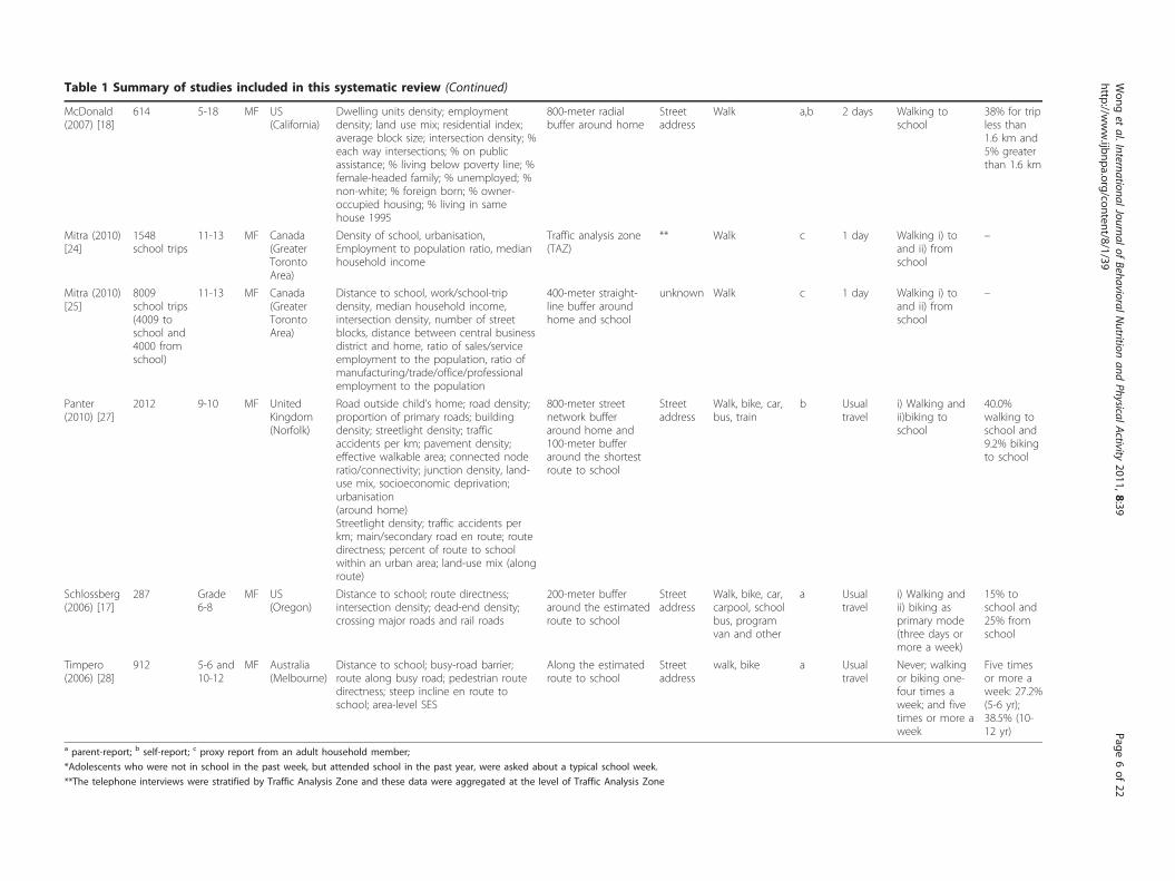
Table 2 Existing built environmental measures
Environmental measures Definition/formula/GIS methods Scale of measuring thevariables
Distance
Distance to school Shortest path to school along the circulationsystem (including roads, trails, and pathways)estimated by GIS/ArcView 3.x extension, NetworkAnalyst V1.0b estimated the distance based onthe shortest route possible along road network
– [17,23,27,28]
Straight-line distance between home and schools – [21,25,26]
Manhattan distance between school and home – [18]
Not reported [29]
Distance to Central Business District Distance between the Toronto Central BusinessDistrict and Traffic Analysis Zone of a respondent’shome
– [25]
Density
Residential/dwelling density The ratio of residential units to the residential area Block group/Traffic AnalysisZone
[16,18,23]
Total number of residents per land area Block group [20,26]
The ratio of total number of residents to theresidential area (and commercial use)
Block group [23,29]***
Residential index Residential units as a percent of dwelling unitsand total employment in the traffic analysis zone
Traffic Analysis Zone [18]
Employment density Number of employees per land area Traffic Analysis Zone [18]
Employment to population ratio Traffic Analysis Zone [24]
Ratio of sales/service employment to thepopulation
Traffic Analysis Zone [25]
Ratio of manufacturing/trade/office/professionalemployment to the population
Traffic Analysis Zone [25]
Number of employees per area of industrial andcommercial land
Unknown [29]
Building density Area of floor space/buildings per land area Study area [27,29]
School density Number of school per land area Traffic analysis zone [24]
Density of school- or work-related trips Walking density-total work and school relatedwalking trips produced by residents in study area
Traffic Analysis Zone [25]
Vehicle density Number of cars and motorcycles per area of roads Study area [29]
Diversity
Mixed land use Land Use Entropy Block group/Traffic AnalysisZone
[16,18,23,29]***
Herfindahl-Hirschman index-proportion of eachland use squared and summed
Not reported [27]
Land use intensity for commercial properties Commercial floor area ratio (FAR) = commercialfloor area/commercial land area
Not reported [19]
Retail floor area ratio Retail building square footage/retail squarefootage
Block group [16]
Design-connectivity-intersections
Intersection density The ratio of number of intersections 3- to 4-wayor 3- to 5-way or not specified) to the land area/street length
Block group/study area [16-18,20,23,27]
Number of major road intersection (3 or 4-way)per land area (primary highway, secondaryhighway and major/arterial roads)
Study area [25]
Number of 4-way local street intersections Study area [25]
Intersection number along the route to school Study area [29]
Percent of 1,3,4, and 5-way intersections Percent of 1,3,4, and 5-way intersections with thebuffer
Study area [18]
Connected node ratio The ratio of number of intersections to number ofintersections and cul-de-sacs
Study area [27]
Wong et al. International Journal of Behavioral Nutrition and Physical Activity 2011, 8:39http://www.ijbnpa.org/content/8/1/39
Page 7 of 22
Table 2 Existing built environmental measures (Continued)
Cul-de-sac density The ratio of number of cul-de-sac to land area Not reported [17]
Design-connectivity-route directness
Pedestrian route directness The ratio of the distance to school along the roadnetwork to the straight-line distance
– [17,27,28]
Design-connectivity-streets
Block/road density Road length (local streets, arterials, and collectors)or number of blocks per land area
Study area [19]***[25,27,29]***
Average block size Not reported Study area [18,29]
Length of each types of road or all streets Total length of motorway, main street, and sidestreet (Switzerland) in each study area
Study area [26]
Proportion of primary road Length of primary roads per length of all roads [27]
Vehicle lane width Average width of vehicle lanes along the route toschool
Study area [29]
Design-sidewalk and bike lanes
Sidewalk/walking tracks length Total length of sidewalk/walking tracks in thestudy area
Study area [23]
Average sidewalk width Not reported Not reported [19]
Average sidewalk width along the route to school Study area [29]
Sidewalk density Proportion of street miles with sidewalk/pavement Study area [19]*** [27]
Percentage length of sidewalks with widths widerthan two metres along the route to school
Study area [29]
Bike lane density Proportion of street miles with bike lanes orpaved shoulders
Not reported [19]
Street spatial design
Across a motorway, main street or a side street/across busy road (freeway, highway, arterial,subarterial, collector, and local road)/across majorroads, or rail roads
Whether the route to school cross these road Along the estimated routeto school/the straight linebetween school and home
[17,26,28]
Route along busy/main or secondary road Whether the route to school along a busy/mainor secondary road
Along the estimated routeto school
[27,28]
Route along
Road outside child’s home A major or minor road adjacent to the child’shome
– [27]
Proportion of primary roads Presence of primary road as part of the route Along the estimated routeto school
[27]
Walkability index
Neighbourhood walkability index Walkability=[(z net residential density) = (z retailfloor area ratio) + (2 × z intersection density) + (zland use mix)]
Cluster of block groups [16]
Individual walkability index Walkability=[(z net residential density) = (z retailfloor area ratio) + (2 × z intersection density) + (zland use mix)]
Study area [16]
Effective walkable area Total neighbourhood area (area that can bereached via the street network within 800 m fromthe home) divided by the potential walkable area(the area generated using a circular buffer with aradius of 800 m from the home)
Study area [27]
Topography and aesthetics
Greenery Proportion of street miles with street trees Not reported [19]
Total number of street trees within 5 m of eachroad edge
Study area [23]
Number of shade trees per the length of route toschool
Study area [29]
Steep incline Altitude between home and school; detail notreported
Along the straight linebetween school and home
[26]
Wong et al. International Journal of Behavioral Nutrition and Physical Activity 2011, 8:39http://www.ijbnpa.org/content/8/1/39
Page 8 of 22
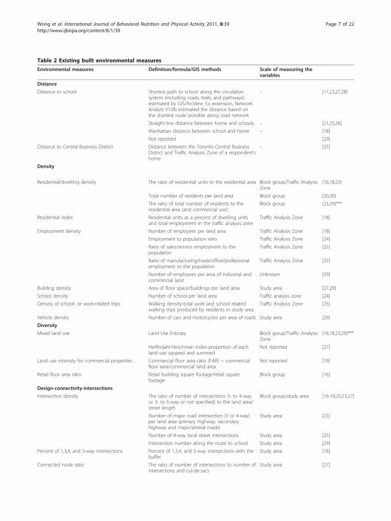
Table 2 Existing built environmental measures (Continued)
A TIN (triangulated irregular network) file wascreated from the digital elevation model (datafrom the State of Victoria). Surface analysis wasundertaken along each route to determine thepresence of a steep incline along any segmentusing Surface Tools, version 1.5.
Along the estimate routeto school
[28]
Average slope gradient within residence area of achild
Not reported [29]
Geographic regions Northeast, South, Mideast, or West in the US – [22]
Urbanisation Population density>4150 persons per square mile(ppsm) = urban; 1000-4150 ppsm = suburban;<1000 ppsm = rural
Not reported [21]
Five levels of urbanisation defined by quintiles ofpopulation density and density of thesurrounding areas: urban, metro suburban, secondcity, town, and rural
Not reported [22]
Urban, inner-suburban, outer-suburban Traffic analysis zone [24]
Urban or rural based on address of child’s home – [27]
Proportion of route to school within an urbanarea
Proportion of route that passes through urbanarea
Along the estimated routeto school
[27]
Safety
Traffic accidents Number of fatal or serious road traffic accidentsdivided by total road length
Study area [27]
Streetlight density Number of streetlights divided by total roadlength
Study area [27]
Demographic-socio-economic status
Area-level socioeconomic status score Based on the Australian Bureau of Statistics’ Indexof Relative Socio-Economic Advantage/Disadvantage
Not reported [28]
Neighbourhood income Median household income Block group/Disseminationarea
[16,23]* [24,25]
Socioeconomic deprivation Population weighted scores for index of multipledeprivation
Not reported [27]
Percent of residents on public assistance Census tract [18]**
Percent of household with income below povertylevel
Block group/Census tract [18]**
Percent of residents unemployed Census tract [18]**
Demographic-education
Educational attainment at neighbourhood level Proportion of population over age 25 years withhigh school diploma
Block group [23]*
Demographic-housing
Percent of residents living in owner-occupiedhousing
Block group/Census tract [18]**
Percent of residents living in the same house as1995
Census tract [18]**
Percent of residents living in female headedhouseholds
Block group/Census tract [18]**
Demographic-ethnicity
Percent of persons born abroad Block group/Census tract [18]**
Percent of non-white residents Block group/Census tract [18]**
Demographic-single parenthood
Single parenthood Proportion of families headed by single parents Block group [23]*
*Canadian equivalent: dissemination area
**Census Tract is a geographic unit comparable to Traffic Analysis Zone which was used to measure other variables.
***Scale of measuring variables is not reported.
Wong et al. International Journal of Behavioral Nutrition and Physical Activity 2011, 8:39http://www.ijbnpa.org/content/8/1/39
Page 9 of 22
our understanding of those processes/forces that areactually responsible for the production of distance.
Diversity: Land use mixFour of the reviewed studies included measures of landuse mix (diversity). In four studies [16,18,23,29], land-use mix was measured using an entropy index, whichquantifies the degree of mixing across land-use cate-gories within a neighbourhood [9]. Some scholars havealso used the Herfindahl-Hirschman index[27]. As ameasure of land use intensity, Ewing et al., estimated,for each parcel, a commercial floor area ratio (FAR)expressed as the ratio of a parcel’s commercial floorarea to the parcel’s land area dedicated to commercialuses [19]. The majority of these studies specified thesource of land-use data: Metropolitan TransportationCommission and Association of Bay Area Government[18], county’s (e.g., Alachua County, Florida) [19] andlocal governmental departments (e.g., City of LondonPlanning Department [23]), and commercial data [27].Three out of fifteen associations between land use mix
and AST were positive [23,29] and the remainder were
null [16,18,19,23,27,29]. Larsen et al. [23] reported sig-nificant positive associations between land-use mix inthe school neighbourhood with AST both to and fromschool, but no association between land-use mix in thehome neighbourhood and AST in youth aged 11-13years. No association between land-use mix and ASTwas observed in children aged 4-18 years [16] or 5-18years [18]. Moreover, Lin et al. report that children liv-ing in an area with mixed land use were more likely toactively commute to school dependently (with an adult)but such an association was not found for trips homefrom school [29].
Density and Diversity: Walkability IndexOne study [16] combined land use, residential density,and connectivity measures to develop a composite walk-ability index. This index, constructed using the followingformula: (z score of net residential density) + (z scoreretail floor area ratio) + (2 × z score intersection den-sity) + (z score land use mix), normalizes the four com-ponents of the walkability index for each block groupusing a z-score. Students who lived in neighbourhoods
Table 3 Summary of GIS data sources used
GIS data sources
Network data
Topographically Integrated Geographic Encoding and Referencing (TIGER)/line street centerline data (US) [17-20]
City of London Planning Department (Ontario, Canada) [23]
The State Government of Victoria (Australia) [28]
Department of Urban Development of Taipei City (Taiwan) [29]
Bicycle and pedestrian level of service database-County’s Geographic Information System (Alachua County,Florida, US)
[19]
DMTI CanMap Route Logistics [25]
Commercial data: Ordnance Survey Integrated Transport Network [27]
Census data (e.g., U.S. Census Bureau/Statistics Canada/Australian Bureau of Statistics, Household RegistrationOffice of Wenshan District (Taiwan), etc)
[20,22-26,28,29]
The Metropolitan Transportation Commission and Association of Bay Area Governments (Alameda, California,US) (land use)
[18]
Property appraiser’s database (parcel layer in county’s GIS) (Alachua County, Florida, US) (land use) [19]
Neighbourhood income [23]d,f [16][23]c,e,f [23]d,e
[25]c,d,e,f
[24]c,d
Socioeconomic deprivation [27]a,b,e
Percent of residents on public assistance [18]j,k
Percent of residents living below poverty line [18]j,k
Percent of residents unemployed [18]j,k
Demographic-education
Educational attainment at neighbourhood level [23]c,d,e,f
Demographic-housing
Percent of residents living in owner-occupiedhousing
[18]j,k
Percent of residents living in the same housesince 1995
[18]j,k
Wong
etal.InternationalJournalof
BehavioralNutrition
andPhysicalA
ctivity2011,8:39
http://www.ijbnpa.org/content/8/1/39
Page12
of22
Table 4 Summary of relationships between GIS-measured environmental factors and AST (Continued)
Percent of residents living in female headedhouseholds
[18]j,k
Demographic-ethnicity
Percent of residents born aboard [18]j,k
Percent of residents being Black [18]j,k
Demographic-parenthood
Single parenthood at neighbourhood level [23]c,d,e,f
Interactions
Neighbourhood walkability × income [16]
Neighbourhood walkability × parental concern [16]
Distance to school × community [26]#
Distance to central business district × blockdensity
[25]c,d,e,##
a walk; b bike; c to school; d from school; e home neighbourhood; f school neighbourhood; g en route; h 5-6 years old; i 10-12 years old; j trip less than 1.6 km; k trip greater than 1.6 km; l dependent travel; m
independent traveln the ratio of manufacturing/trade/office/professional employment to the population; o the ratio of sales/service employment to the population
*In U.S., adolescents living in South region were less likely to actively commute to school than those in Northeast region.#The strongest relationship between distance between home and school on AST was found in Biel (German-speaking) followed by Biel (French-speaking) and Bern.##Children living in a neighbourhood with smaller blocks and located far from the central business district were less likely to walk than those living in a place with larger blocks and located closer to the centralbusiness district.
Wong
etal.InternationalJournalof
BehavioralNutrition
andPhysicalA
ctivity2011,8:39
http://www.ijbnpa.org/content/8/1/39
Page13
of22
with a higher walkability index were more likely toactively commute to school [16]. In high walkabilityneighbourhoods, children with high socioeconomic sta-tus were more likely to actively commute to school thanthose with low socioeconomic status [16]. Similarly,children from households with low parental concernabout safety and barriers in a high walkability neigh-bourhood were more likely to actively commute toschool than their counterparts [16].
Street Design: Intersection and dead-end densitiesEight studies measured intersection density [9] by divid-ing number of intersections by the area of spatial unitsused in the analysis (e.g., 200-meter buffer along theroute to school [17], 400-meter [25], 500-meter [23],800-meter [27] or 1-km buffer around home[16], 1.6-kmbuffer around school [23] or traffic analysis zones[18])[16-18,23,25,27] or by dividing the number of intersec-tions by the length of a road segment [20]. Lin et al.examined the number of intersections along the routeto school [29]. Intersections were defined in differentways: 3-way or more [16,25], 3- and 4-way [17,23], andundefined [18,20,27,29]. Most studies reported the dataused for measuring intersection density (e.g., street cen-terline/road network data [17,18,20,23,25,29]). Besidesintersection density, Schlossberg et al. measured theratio of number of dead-ends to the area of the 200-mbuffer along the shortest route to school [17]. In studieswhere the relationship between intersection density andAST has been described, null relationships werereported in eighteen of twenty cases[16-18,20,23,25,27,29]; the remaining two cases reporteda negative association [17,29]. No association betweenintersection density and AST was observed for youthaged 9-10 years [27] or 11-13 years [23,25] or for chil-dren aged 4-18 years [16] or 5-18 years [18]. However,Schlossberg et al. [17] found a negative associationbetween intersection density and walking, but not bik-ing, to school in grade 6-8 students. Lin et al. [29]found a similar association but only with independent(unescorted) active school transport in the morning.
Street Design: Use and Route DirectnessPedestrian route directness [31], a connectivity measuredefined as ratio of the shortest estimated distance toschool along the road network to the straight-line dis-tance, was measured in two studies. Street centerlinedata [17-20], governmental data [23,28,29] and in onestudy commercial data (Ordnance Survey MastermapTransport Network, UK) [27], was input to a GIS forthe purpose of estimating numerator data using a short-est path network analysis algorithm.In these studies [17,27,28], three of the six associations
between route directness and AST were negative and
the remainder null, meaning that some studies havedemonstrated that the requirement for a child to take arelatively indirect route to school typically associateswith the use of some form of motorized transportation(typically the private car). Timperio et al. [28] found asignificant negative association between route directnessand AST in youth aged 10-12 years. The direction ofassociation was the same for children aged 5-6 years butnot significant [28]. Panter et al. also reported suchnegative associations in youth aged 9-10 years. Schloss-berg et al. [17] did not report any association for middleschool students.
Street Design: Blocks, Street Length and Availability ofActive InfrastructuresAverage block size [18,29], length and density of streetsegments (e.g., main and side streets) in the studiedsites (buffer areas of 200 m around the route to school)in the buffer of estimated route to school (straight linebetween school and home) [26], and street density[19,25,27] in the study area were measured. Only five offourteen associations between street-related variablesand AST were positive and the remainder were null.One study reported associations of street density withwalking independently (unescorted) to school anddependently (escorted or with other children) backhome [29]. Similarly, Mitra et al [25] reported that chil-dren living in an area with higher block density weremore likely to walk to school, the relationship did nothold for the trip home from school. Studies thatreported associations between street-related variablesand AST tend to include younger children and narrowerage groups (9-13 years) [25,27,29] whereas studies thatfailed to report such associations tended to include stu-dents from kindergarten to grade 12 [18,19].Ewing et al. [19] used the Alachua county’s bicycle
and pedestrian level-of-service database to assess theproportions of street length with bike lanes and side-walks, average sidewalk width and sidewalk coverage.Similarly, sidewalk completeness (the total length ofsidewalk/walking tracks in the study area) was examinedin another study [23]. Larsen et al. [23] created a ‘circu-lation system’ database by combining the digital maps ofroad network, trail network, and informal pathways/footpaths, a composite approach that assesses the total-ity of pedestrian infrastructure (planned and unplanned).No associations were found between densities of bikelanes and sidewalks, average sidewalk width and AST[19,23]. Moreover, Larsen et al. [23] did not find anyassociation between sidewalk completeness and AST inyouth aged 11-13 years. In a separate study however,sidewalk coverage was positively associated with schooltrips by walking but not by biking [19], and with walk-ing independently to school but not back home [29].
Wong et al. International Journal of Behavioral Nutrition and Physical Activity 2011, 8:39http://www.ijbnpa.org/content/8/1/39
Page 14 of 22
Street Design: Competing Uses and LocationFour studies [17,26-28] examined whether busy roads (e.g., collectors, highways, freeways, rail road, major roads,and arterial) were along or cut across the shortest pathestimate of a students’ route to school. The findingswere mixed. Children aged 5-6 years and youth aged 10-12 years with busy road barriers (freeways, highways, orarterial roads crossing) along their route to school wereless likely to walk or cycle to school [28]. Similarly,Bringolf-Isler et al. [26] observed a positive associationbetween main street crossings along a school route andnon-active commuting in children in aged 6-14 years. Inother studies no associations were found betweenmotorway location, side streets, and railroad trackscrossing the school route and AST [17,26]. Panter et al.[27] reported a negative association between the pre-sence of a main road along the school route and walkingor biking to school, while Timperio et al. [28] did notfind an association between the presence of a busy road(freeways, highways, or arterial roads) along the schoolroute and AST.
Street Design: AestheticsThree studies measured aesthetics in terms of treesplanted along roads [19,23,29]. In one study, trees alongroads were counted within 5 meters from road edges inthe study area using data from London’s Street TreeInventory [23]. Another study measured the proportionof street miles with street trees using the AlachuaCounty, Florida bicycle and pedestrian level-of-servicedatabase [19]. A third approach involved counting thenumber of trees with shade along the estimated route toschool [29].One out of five associations with AST was positive
and the remainder were null [19,23,29]. Larsen et al.[23] found an association between number of streettrees within 5 m of the road edge and active commutingto school but not back home for youth aged 11-13years. Ewing et al. [19] reported no association betweenproportion of street length with street trees and walkingand biking for children and youth ranging from kinder-garten to grade 12.
Street Design: TopographyThree studies examined topography, more specifically,the slope of streets [26,28,29]. Timperio et al.[28] esti-mated slope associated with school routes by conductinga GIS-based terrain analysis of the study area. A Trian-gulated Irregular Network (TIN) can be created by fit-ting a set of non-overlapping triangular facets to a set ofirregularly spaced elevation points. This approach cre-ates a vector-GIS representation of terrain from whichtopographic data can be estimated including slope (rateof change in elevation) and aspect (the direction of
maximum gradient). Timperio et al. used the TINapproach to assess the slope of school routes, with aview to determining the presence of a steep inclinealong any road segment that is part of the set of seg-ments that comprises a student’s school travel route[28]. Timperio et al.[28] found a negative associationbetween the steep slope along the route to school andAST in children aged 5-6 years but not in youth aged10-12 years. Elsewhere, no association between steepslope along the route and AST among youth aged 6-14years was found [26] while Lin et al.[29] also reported anegative association between steep slope and walkingback home independently (unescorted) but not to schoolin elementary school students. Specific informationabout how slope was modeled in these two studies wasnot provided.
DiscussionThere is currently no consistent evidence supporting theassociation between GIS-measured aspects of the builtenvironment with AST except distance to school. It isimportant to consider that distance between home andschool is produced by interactions between complexsocial and economic processes that influence home andschool locations. For example, and with sufficient capi-tal, people may select themselves into neighbourhoodsas an expression of preference for a certain bundle ofamenities and services. This process of self-selectioncould produce residential choices at either end of thesustainability spectrum. Conversely, others may experi-ence a household mobility process where the choice ofalternatives is limited to the availability of social-housingat fixed locations across a city, and/or vacancies at thelower end of the rental or owner segments of the hous-ing market. In short, the residential choice process, andhousing policy more broadly, has an important role inproducing school travel distance.There was less consistent evidence that land use mix
and density and connectivity (intersections) were relatedto AST, although some studies did find a positive rela-tionship. Other variables such as having a busy roadcrossing or a busy road located along the route toschool; greenery; or composite metrics of neighbour-hood walkability have been less frequently assessed, yetin some instances there were either positive, negative ornull relationships reported across studies. Does thismean that objective measurement of the built environ-ment is not important to understanding AST? It is pre-mature for such a conclusion at this stage given some ofthe methodological challenges inherent in this type ofresearch; the possibility that some important features ofbuilt environment have not been assessed; the likelihoodthat the relationship between the built environment andschool travel may indeed be different in different cities,
Wong et al. International Journal of Behavioral Nutrition and Physical Activity 2011, 8:39http://www.ijbnpa.org/content/8/1/39
Page 15 of 22
regions, and or neighbourhoods; and that the relation-ships between the built environment and AST may bemoderated significantly by a range of other factors suchas the age of children and youth, time of day, trip typeor chains (e.g., the presence of activities before or afterthe school trip) or school travel mode.
Theoretical and Methodological IssuesSubjective environmental measures reflect subjects’ per-ception. Without understanding the process throughwhich subjects experience and interpret their actualenvironment, the use of objective environmental mea-surement (e.g., GIS) to assess the effect of BE on ASTremains a necessary and complementary methodologicalapproach for understanding this relationship. Despitethe importance of GIS measures, there were a numberof theoretical and methodological limitations within thecurrent literature including inconsistencies in geocoding,selection of study sites, buffer methods and sizes andthe shape of zones (the Modifiable Areal Unit Problem[MAUP]), the quality of road and pedestrian infrastruc-ture data, estimation of the route to school, and incon-sistency in applying measures of the built environment.These limitations reflect challenges both in terms ofthinking about the spatial science/theory underlyingAST research, and the pragmatic/technical understand-ing of how to apply GIS software.First, the geocoding issue refers to the accuracy with
which a researcher can pinpoint the location of a sub-ject’s home location on a digital map of the built envir-onment. This geocoding accuracy issue is moderated byboth ethical (i.e., a research ethics board ruling aboutthe use of personal information), and methodological (i.e., data availability) considerations. Moreover, researchparticipants might be reluctant to offer street addresslocations to researchers. Measures of the built environ-ment attached to a subject’s home location could subse-quently suffer from measurement error when thesubject’s home location has not been accurately geo-coded. Despite this concern, only one study reportedthe geocoding method (e.g., postal code geocoding) [23]whereas more commonly, geocoding methods were notreported [16-19,21,22,25-29]. Larsen et al. [23] geocodedstudents’ home based on postal code. However, 25% and20% of postal code locations were beyond 200 m of theactual street address location; postal code geocodingplaces subjects within a postal code zone, not at theactual location along the street system [32]. Larsen andcolleague’s use of a 500 m buffer may have led to sub-stantial error. The issue of compounding error and spa-tial uncertainty in the location data used in ASTresearch has not been adequately discussed in the litera-ture. Studies that address the sensitivity of experimentalresults to the geocoding issues are warranted.
Second, a common practice across studies is to gener-ate buffers around home, school, and occasionally routelocations, and then to measure the built environmentwithin the buffered objects, using one or more of theapproaches described earlier. The expectation is that thepresence of enabling infrastructures within buffers, thatare often used as a metric for the concept of neighbour-hood, will produce active travel outcomes. The primarytheoretical concern with regard to buffer analysisinvolves the specification of buffer methods and size, aprocess that is subject to the Modifiable Areal Unit Pro-blem (MAUP) [33]. MAUP occurs when the results ofdata analysis exhibit sensitivity to the geometry (e.g.,size, shape) of spatial units (e.g., census zones) used forthe reporting of data input to the analysis process. Thereference to modifiable areal units reflects the fact thatit is quite often the case (particularly with secondarydata) that the spatial units under analysis may be arbi-trary constructs of a data collection and aggregationprocess, conducted usually by a third party, with a viewto developing spatial units for statistical reporting [33].The use of buffers in the measurement of built environ-ment characteristics is an example of an analytical pro-cess where relatively arbitrary decisions are takenregarding the shape (i.e., AST research usually appliescircular buffers, this need not be the case) and size ofbuffers. The buffer approach is an area-based approachto ascribing built environment qualities to individualcases, because built environment characteristics are esti-mated within the areal unit of a buffer, these types ofmeasures are likely subject to the MAUP. There hasbeen some discussion of the intersection betweenMAUP and area-based measures included as indepen-dent variables in the multivariate analyses of discrete orcontinuous outcomes [34,35]. An example to illustratethis issue is presented by Lee’s study [36].MAUP includes two effects: scale and zoning or
aggregation effects [33]. The scale effect is the varia-tion in results due to the size of areal units used in theanalysis of a given area, which consequently associateswith the number of areal units required to exhaustivelycover a study area [33]. For example, associationsbetween the built environment and school travel modemay differ between a 400 m or 800 m buffer surround-ing the place of residence for the same set of cases.The definition of these units, in this case, the buffers,is arbitrary and modifiable, and hence measures of thebuilt environment derived from buffer analysis, such ascounting the number of intersections within a bufferand dividing by the buffer area to generate a measureof intersection density, could change with adjustmentsto the buffering procedure selected by the researchers.The inconsistency of buffer sizes also makes cross-study comparison difficult. In the reviewed studies,
Wong et al. International Journal of Behavioral Nutrition and Physical Activity 2011, 8:39http://www.ijbnpa.org/content/8/1/39
Page 16 of 22
buffer sizes varied from 400 m [25], 800 m [20] or 1.6km [23] buffers around schools, no buffers [28] or 100m [27] or 200 m [17,26] buffers around the route toschool, 400 m [25], 500 m [23] or 800 m buffers sur-rounding home [18,27]. Kerr et al. [16] measured theneighbourhood at two-levels: block group and a moreproximal one (1 km buffer). One study did not reportthe spatial units used to measure the built environ-ment characteristics [29]. Moreover, different methodswere adopted: Euclidean [17,18,20,23,25,26] and net-work buffer [16,27]. Based on the original work of Leeand Moudon [10] reflected in the framework describedby Panter [7], environments around home, school anden route all impact decision-making on children’s AST,and hence it is important to investigate the combinedeffect of these places and routes on AST. There is,however, an additional statistical issue that requiresconsideration. In cases where buffers around objectsoverlap, either because a generous radial distance wasselected for buffer creation, or because the bufferedobjects are simply located very close to one another (e.g., a short school trip), objectively measured builtenvironment data may be highly correlated, an issuethat has not been widely discussed [25].The zoning or aggregation effect refers to how analyti-
cal results may vary when scale is maintained (e.g., thenumber of units is consistent) but the partitioning (geo-metry) of the units is adjusted. For example, estimatedAST rates for a set of ten traffic zones may be very dif-ferent when the boundaries for each zone are adjustedto include and/or exclude individual cases. The zoningeffect is a geographical problem that has remained hid-den from view in AST studies that have made use ofexogenously and arbitrarily constructed systems of cen-sus or traffic zones for the reporting of either builtenvironment data or school travel mode share. Cur-rently, there is no universal solution for MAUP; andarguably, it is quite useful to conduct policy-based ana-lysis using systems of zones embedded within the dis-course surrounding the particular policy issue (i.e., if aschool board is evaluating transport policy within aschool district, then reporting empirical results at thatscale is likely to be the most policy relevant course ofaction). However, using the most spatially disaggregateddata, and demonstrating the sensitivity of the results toboth scale and zoning effects increases confidence thatthe results at the most disaggregated level have somemeaning and are not simply the artefact of the ways inwhich data are being arranged [37]. Surprisingly therehas been no theoretical or empirical engagement withthis issue in the AST literature.Third, missing pedestrian data [38] and inaccuracy
and incompleteness of street network data [39] couldlead to inaccurate measurement of connectivity and the
estimation of routes actually used by pedestrians. In thisreview, using street network data to measure connectiv-ity (e.g., route directness) and pedestrian infrastructureswas common [17,28]. However, street network data didnot typically include pedestrian options other thanstreets (e.g., paths or trails). Incomplete pedestrian data(e.g., street centerline network data likely does notinclude paths or trails that pedestrians could walk) cre-ates uncertainty with respect to measuring connectivityand therefore calls into question what we actually knowabout the empirical relationship between connectivityand AST. In addition, one study [39] reported variationsin the quality of road network datasets in terms of com-pleteness, accuracy, and currency, demonstrating theimportance of examining the quality of available roaddatasets. If necessary, they suggest customizing the data(e.g., by updating with aerial photographs and tax par-cels and fieldwork with GPS [39]).Fourth, the actual route to/from school taken by study
subjects has not been assessed in the reviewed studies.Five studies examined the impact of the BE along stu-dents’ route to school on AST [17,26-29]; however, theyused a network shortest path route from a GIS to esti-mate the route to school. The estimated route, based onthe assumption of minimizing the generalized cost ofthe trip measured in terms of total time or network dis-tance, may not be the actual route taken by the subjects.It is common that children (encouraged by caregivers ornot) may look to organize themselves with other chil-dren on the way to/from school, this organizational pro-cess during the trip may indeed require the use oflonger routes than predicted by a shortest path algo-rithm. Duncan et al.[40] found that the route measuredby GPS or GIS were comparable in terms of distance;however, the quality and/or spatial structure of theroute was significantly different [40]. That is, the actualroutes tended to be less busy, and the data suggest dif-ferences in the intersections, turns, and segments tra-versed. The route distance to school estimated by GISmay be a good proxy but the geography of the shortestroute data may not match with the actual route takenby research participants. As a result, measures of builtenvironment characteristics taken within a bufferaround a shortest route may not accurately reflect thebuilt environment characteristics that a subject actuallyexperiences. Of course, the shortest path does controlfor the street architecture, something that is not con-trolled for at all when applying the Euclidean or Man-hattan metrics. Interestingly then, none of the reviewedstudies reported the validity of the application of theshortest path approach (e.g., mapping activities or theuse of GPS could be used to validate such an approach).Fifth, there is inconsistency in how GIS measures of
the built environment are applied. An example is land
Wong et al. International Journal of Behavioral Nutrition and Physical Activity 2011, 8:39http://www.ijbnpa.org/content/8/1/39
Page 17 of 22
use measures. Land use measures used in included stu-dies are entropy [16,18,23,29], Herfindahl-HirschmanIndex [27], and a commercial floor area ratio (FAR)[19]. The typical entropy approach to measuring landuse mix can be expressed using the following formula:
E = −[∑
jpj ln pj]/ ln k
where pj is the proportion of land in use j and krepresents the total number of land uses (single family,multi-family, retail/service, and manufacturing/trade/other). The result is an index ranging between zero (sin-gle use) and one (mixed land use) [9]. The Herfindahl-Hirschman index was calculated by:
HHI(K) =K∑
i=1
(Pi · 100)2
where K is the number of land use types, and Pi is thepercentage of each land use type (e.g., farmland, wood-land, grassland, uncultivated land, other urban, beach,marshland, sea, small settlement, private gardens, parks,residential, commercial, multiple-use buildings, otherbuildings, unclassified buildings, and roads) within thestudy area [27]. As a measure of land use intensity, acommercial floor area ratio (FAR) was expressed as theratio of a parcel’s commercial floor area to the parcel’sland area dedicated to commercial uses [19].In summary, inaccurate geocoding, inconsistent selec-
tion of study sites, buffer methods and sizes, poor qual-ity of road and pedestrian infrastructure data, inaccurateestimation of the route to school, and inconsistent appli-cation of measures of BE attributes were the main meth-odological challenges identified in the current literature.These challenges are not easily addressed. Standardisingthe operational definition of neighbourhood and exam-ining the impact of various buffer size on the relation-ships between BE and AST should be considered infuture studies. Future studies should attempt to custo-mise road and pedestrian infrastructure data, if neces-sary and feasible, to improve quality. Measuringstudents’ route to school may be performed more accu-rately with GPS or by asking the subjects (or guardians)to map their route to school and then digitising to GIS[41] although these approaches are not without limita-tions (e.g., lack of signal or signal dropout [40] of GPSor misreading the map by the subjects, not to mentionthe resource-intensive nature of compiling such data).
Are we measuring the right thing?According to frameworks by McMillan [6] and Panter[7], the built environment may influence parents’ or/andchildren’s environmental perception which in turn mayinfluence school transport behaviours. It is possible that
features of the built environment currently assessed byGIS are not relevant to parents. It is important to com-pare whether the perceived environment is more expla-natory than the actual environment in predicting AST.One study examined the effect of parent’s and children’sperceived environment and objectively-measured builtenvironment with AST [28]. Similarly, another study[16] examined whether parental concern and perceivedenvironment explained the association between the builtenvironment and AST. In a ‘combined’ model, percep-tions regarding the presence of walk and bike facilities,and the perceived availability of stores within a 20 min-ute walk remained positively associated with AST, whilean objective walkability index did not associate withAST. This may suggest that perceptions of environment,which are incidentally partially a response to the “built”environment presented to the subject, are more power-ful predictors than objective measures. However, theself-report and objective measures of built environmentdid not measure the same thing (e.g., self-report of hav-ing no streetlights and objective measure of the routealong a busy road in Timperio’s study [28], and objec-tive walkability index [42] and self-report of the pre-sence of walk and bike facilities in Kerr’s study [16]). Itis difficult to compare the independent effects on AST.More specifically, “people’s perceptions may, in fact,motivate their behaviour more than the true nature ofthe situation” [15]. Despite this, both parental percep-tion of the environment and the actual environmentmay have independent effects on AST decisions. There-fore, in future studies, it is important to ideally combineobjective measurement of the environment with the per-ceptions of parents and children through self-report. Tothis end, there is likely a need to work on advancing ourunderstanding of how to describe the built environmentin non-technical terms to study subjects, using conceptsand language that can be translated again back into theframes of reference applied to the planning and engi-neering of neighbourhoods and cities.It is also important to identify features of the built
environment that have not yet been examined but maybe important. For example, perceived safety-related vari-ables may be critical (e.g., reaction to the presence/absence of pedestrian and cycling infrastructure [7,8],controlled intersection (e.g., crossing or green lights atintersections) [11,28], and parental and adolescent safetyconcerns [7]) may have an effect on AST. While safetyis acknowledged as an important factor in the generalAST literature [3], few studies have looked to examinethis construct using GIS derived variables. Only tworeviewed studies examined busy roads crossing [17,26]/along [27,28] the route to school as indicators of roadsafety. Only one study examined the effect of density oftraffic accidents on walking or biking to school;
Wong et al. International Journal of Behavioral Nutrition and Physical Activity 2011, 8:39http://www.ijbnpa.org/content/8/1/39
Page 18 of 22
however, no associations were found [27]. Different roadsafety indicators should be examined in future research.Some road safety indicators in studies on youth’s generalactive transportation or school neighbourhood walkabil-ity such as roads with speed humps, chicanes and sec-tions of intentionally narrowed road, and traffic lights[43], average annual daily traffic volume, and percent ofhigh-speed streets [44] could be applicable to the con-text of AST.Another safety-related variable, self-reported presence
of a controlled intersection (e.g., intersections withcrossing and green lights), which was found to be asso-ciated with AST [28], has not been examined objectivelyusing GIS. No association was found between GIS-mea-sured intersection density and AST in the reviewed stu-dies. This finding may be attributed to all streets beingincluded (e.g., busy arterials and local streets). However,crossing busy roads (intersections with busy roads) maybe considered as a traffic danger and may reduce thelikelihood of actively commuting to school if childrenhave to use these intersections. Measuring connectivitywithout major roads [45] may be more suitable in ASTresearch. For child pedestrians, routes to school usingminor roads with less traffic volume and lower speedlimits tend to be chosen [40].Consideration should be given to the hierarchical con-
struction of road networks and the relationship betweenthe different levels of the hierarchy (e.g., large arterialswith fast moving traffic, to local streets with sidewalks),and AST outcomes (see for example [46]). Two studiesexamined the effect of intersection density withoutmajor streets [27] or with local streets only [25] onAST; however, no association was found. There is morework to be done on the links between roadway hierar-chy and AST. Measuring connectivity, and potentiallyroute directness, without major roads may reflect moreappropriately the walkable options that parents wouldallow their children to take. Besides road safety, parentalconcerns of safety includes personal safety as well [7]although none of the reviewed articles examined perso-nal safety. The spatial analysis, using GIS, of crime data[44] could be an option in this context.The frameworks by Panter et al. [7] and Lee and
Moudon [10] highlighted the importance of examiningthe effects of the two trip-ends (home and school) andtheir surrounding neighbourhoods and the route toschool on AST. Only one study in this systematic reviewexamined the neighbourhood surrounding home, schoolcharacteristics, and the environment surrounding theroute to school [27]. The high ratio of intersections tointersections and dead-ends, low road density, and highsocioeconomic deprivation in the neighbourhood sur-rounding home were negatively associated with walkingto school whereas long distance to school, high route
directness, and main route along the route were nega-tively associated with walking to school. No associationsbetween school characteristics (e.g., presence of a schooltravel plan, walking bus scheme, cycle path, and pedes-trian crossings which were measured by questionnairecompleted by head teachers and research audit) andwalking to school were observed; however, the neigh-bourhood surrounding schools was not assessed. Mitraet al. [21] reported distinct effects of the neighbourhoodsurrounding school and home on school transport.Findings from these two studies suggest that the builtenvironment surrounding home and school and alongthe route to school may have distinct effects on schooltransport. Future studies on school transport shouldconsider the neighbourhood surrounding the two trip-ends (school and home) and along the route to school.In summary, some of the suggested variables (e.g.,
controlled intersections-with green lights or crossing)have not been studied or have been only studied once(e.g., busy road crossing the route to school). Future stu-dies should consider exploring safety further usingobjective measurement (e.g., intersections with greenlight, streets with crossing, speed humps, overhead streetlights, average annual daily traffic volume, crash rates,crime rates); confirming the spatial design of street net-works (e.g., busy roads crossing the buffers or nearestdistance to a busy road); modifying connectivity mea-sures (e.g., comparing intersection indicators with andwithout removing the busy roads and re-examining theconnectivity with improved pedestrian and cyclist infra-structures including pathways, trails, bike lanes, etc.);examining environmental features along respondents’route to schools, and assessing neighbourhoods sur-rounding both school and home and along the route toschool.
Potential modifiersIn addition to the theoretical and methodological chal-lenges in applying GIS to the examination of the builtenvironment and school transport, our findings alsosuggested that there may be several potential modifiersof any relationship including: age, direction of the route,and travel mode. First, there is the need for researchersto make a distinction between the trip to school, andthe trip from school [4]. Larsen et al. [23] observedassociations of residential density and street trees alongthe road in the home but not school neighbourhoodwith AST. However, different buffer sizes applied toschool (1.6 km) and home (500 m) make it difficult tointerpret the findings as to whether the built environ-ment has different effects on different school trips orwhether the findings are attributed to differences in buf-fer size (i.e., MAUP effects). However, the finding doeshighlight the possibility that the influence of the built
Wong et al. International Journal of Behavioral Nutrition and Physical Activity 2011, 8:39http://www.ijbnpa.org/content/8/1/39
Page 19 of 22
environment varies temporally. For example, Mitra et al.found an association of density of schools with clustersof high AST only in the morning and an association ofemployee density with clusters of high AST only in theafternoon [24]. In another study, Mitra et al. [25] foundthat more built environment variables were associatedwith walking in the morning than in the afternoon. Thetemporal variation in associations between the builtenvironment and active school transport may beexplained by parental/caregiver schedules (e.g., work)and resource availability. For example, parents may beavailable to drop their children off along their way towork; however, these working parents may not be avail-able to pick their children up after school [47]. Thiscould lead to the mode shift from passive in the morn-ing to active in the afternoon. Besides temporal varia-tion, the association between built environment trip andschool transport may vary between trip-ends (e.g.,school and home neighbourhoods). The built environ-ment near the location of residence has been shown tobe more strongly correlated with mode choice than thebuilt environment around the school [25].Second, half of the reviewed studies combined chil-
dren and adolescents in analyses [16,18,19,26]. The asso-ciation between number of street trees within 5 m ofroad edge and active commuting to school was observedin youth aged 11-13 years [23]. In contrast, Ewing et al.[19] failed to find such an association for kindergartento grade 12 students. A significant negative associationbetween the steep slope along the route to school andAST was found in children aged 5-6 years but not aged10-12 years [28]. No association between steep slopealong the route and AST was observed among youthaged 6-14 years [26]. This suggests that the effect ofbuilt environmental features on AST may vary not onlyacross age but within narrow age groups (e.g., early ele-mentary students, late elementary students, middleschool students, and high school students [able todrive]).Third, the effect of environmental features on biking
and walking are likely to be different. These modesrequire different levels of investment by private andpublic stakeholders in equipment and infrastructure,they typically operate using different parts of the roadsystem, require different skill sets, and the developmentof the necessary infrastructure may be operationallyembedded within very different and sometimes highlycontested planning processes. Ewing et al. [19] found apositive association between sidewalk density and walk-ing to school but not biking to school. Similarly,Schlossberg et al. [17] reported a positive associationbetween intersection density and walking to school butnot biking to school. However, it is uncommon toexamine biking and walking separately (only two studies
in this review did so [17,19]). For example, the effect ofsteep slope on biking and walking to school may be dif-ferent. In one of the reviewed studies, steep slope wasfound not to be associated with overall AST [26]. InCanada, few students cycle to school [4] and hence itmay not be possible to examine this interaction in theCanadian context, at the population level. However, inEuropean countries where cycling is more prevalent,researchers should consider the interaction betweenactive travel modes and the built environment. In gen-eral, the evidence that is available, coupled with ourunderstanding of the planning and practice of walkingand biking raises valuable questions about the efficacyof modelling walking and biking together as a singlemode category.In summary, potential modifiers include age (e.g., mid-
dle school students and high school students), schooltravel mode (e.g., walking and biking), direction of route(e.g., to school and from school), and trip-ends (homeand school). Important associations between the builtenvironment and school travel mode may be attenuatedif these modifying variables are not controlled for.Hence, it is important for future studies to examinetheir potential interactions with the built environment.If interactions are found, they should be analysedseparately.
ConclusionsThe application of GIS to the study of AST is relativelynew, but informed by more than a decade of workwhere GIS has been applied in studies of adult travelbehaviour and urban form. Aside from distance, com-monly assessed features of the built environment arenot consistently related to AST although we acknowl-edge that some relevant studies may have been excludedif they were unpublished or not in the English language.Numerous methodological challenges exist includinginconsistencies in geocoding, selection of study sites,buffer methods, and sizes, incomplete road and pedes-trian and cyclist infrastructure data, and inaccurate esti-mation of the route to school. The use of differentdefinitions applied to similar environment features (e.g.,number of intersections per unit of area vs. percentageof particular type of intersection [for example, 3-way] orstreet density vs. total street length) makes it difficult tocompare studies. To facilitate international comparison,including generic measures such as the walkabilityindex, is recommended in future research. Futureresearch should also attempt to a) standardize buffermethods and explore the impact of different buffer sizeson the associations between the built environment andAST, including both school and home neighbourhoods;b) customize the road and pedestrian and cyclist infra-structure data to improve quality; c) measure the actual
Wong et al. International Journal of Behavioral Nutrition and Physical Activity 2011, 8:39http://www.ijbnpa.org/content/8/1/39
Page 20 of 22
route to/from school with more accurate measurement(e.g., GPS or map drawing); d) include both objectiveand subjective measures of the built environment; ande) consider the potential interactions of age, trip direc-tion, and travel mode with the built environment mea-surement. While such rigor may not always be possiblegiven the accompanying resource demands, future stu-dies certainly need to report greater methodologicaldetail to facilitate replication.
AcknowledgementsThis review was funded by the Built Environment, Obesity and HealthStrategic Initiative of the Heart and Stroke Foundation of Canada and theCanadian Institutes of Health Research (CIHR).
Author details1Faculty of Physical Education & Health, University of Toronto. 2Departmentof Geography, University of Toronto Mississauga.
Authors’ contributionsBYW conducted the literature search, data extraction, literature screen, anddata analysis and wrote the initial draft of manuscript. GF and RBparticipated in literature screening, analysis, providing methodological input,and in the writing of the manuscript. All authors read and approved thefinal manuscript.
Authors’ informationBYW is a doctoral candidate in the Faculty of Physical Education and Health,University of Toronto and is a CIHR/HSFC Fellow in Population Intervention forChronic Disease Prevention. GF is an Associate Professor in the Faculty ofPhysical Education and Health, University of Toronto. RB is an AssistantProfessor in the Department of Geography, University of Toronto.
Competing interestsThe authors declare that they have no competing interests.
Received: 28 July 2010 Accepted: 6 May 2011 Published: 6 May 2011
References1. Tremblay MS, Shields M, Laviolette M, Craig CL, Janssen I, Gorber SC:
Fitness of Canadian children and youth: Results from the 2007-2009Canadian Health Measures Survey. Statistics Canada Health Reports 2010,21:1.
2. Faulkner GE, Buliung RN, Flora PK, Fusco C: Active school transport,physical activity levels and body weight of children and youth: asystematic review. Prev Med 2009, 48:3-8.
3. Sirard JR, Slater ME: Walking and bicycling to school: A review. AJLM 2008,1559827608320127.
4. Buliung RN, Mitra R, Faulkner G: Active school transportation in theGreater Toronto Area, Canada: an exploration of trends in space andtime (1986-2006). Prev Med 2009, 48:507-512.
5. Blair S, Clark D, Cureon K: Exercise and fitness in childhood: implicationsfor a lifetime of health. In Perspective in exercise science and sportsmedicine: youth, exercise and sport. Edited by: Gisolfi C, Lamb D. Indianapolis(IN): Benchmark Press; 1988:401-430.
6. McMillan TE: Urban form and a child’s trip to school: The currentliterature and a framework for future research. J Plann Lit 2005,19:440-456.
7. Panter JR, Jones AP, Van Sluijs EM: Environmental determinants of activetravel in youth: A review and framework for future research. Int J BehavNutr Phys Act 2008, 5:34.
8. Pont K, Ziviani J, Bennett S, Wadley D, Abbott R: Environmental correlatesof children’s active transportation: A systematic literature review. HealthPlace 2009, 15:827-840.
9. Cervero R, Kockelman K: Travel demand and the 3Ds: Density, diversity,and design. Transport Res D Tr E 1997, 2:199-219.
10. Lee C, Moudon AV: Physical activity and environment research in thehealth field: Implications for urban and transportation planning practiceand research. J Plann Lit 2004, 19:147-181.
11. Davison KK, Werder JL, Lawson CT: Children’s active commuting to school:current knowledge and future directions. Prev Chronic Dis 2008, 5:A100.
12. Schlossberg M, Phillips PP, Johnson B, Parker B: How do they get there? Aspatial analysis of a “sprawl school” in Oregon. PPR 2005, 20:147-162.
13. Falb MD, Kanny D, Powell KE, Giarrusso AJ: Estimating the proportion ofchildren who can walk to school. Am J Prev Med 2007, 33:269-275.
14. Ferreira I, van der Horst K, Wendel-Vos W, Kremers S, van Lenthe FJ, Brug J:Environmental correlates of physical activity in youth: a review andupdate. Obes Rev 2007, 8:129-154.
15. Davison KK, Lawson CT: Do attributes in the physical environmentinfluence children’s physical activity? A review of the literature. Int JBehav Nutr Phys Act 2006, 3:19.
16. Kerr J, Rosenberg D, Sallis JF, Saelens BE, Frank LD, Conway TL: Activecommuting to school: Associations with environment and parentalconcerns. Med Science Sports Exerc 2006, 38:787-794.
17. Schlossberg M, Greene J, Phillips PP, Johnson B, Parker B: School trips -Effects of urban form and distance on travel mode. J Am Plann Assoc2006, 72:337-346.
18. McDonald NC: Travel and the social environment: Evidence fromAlameda County, California. Transport Res D Tr E 2007, 12:53-63.
19. Ewing R, Schroeer W, Greene W: School location and student travel:Analysis of factors affecting mode choice. Transport Res Rec 2004,1895:55-63.
20. Braza M, Shoemaker W, Seeley A: Neighborhood design and rates ofwalking and biking to elementary school in 34 California communities.Am J Health Promot 2004, 19:128-136.
21. Babey SH, Hastert TA, Huang W, Brown ER: Sociodemographic, family, andenvironmental factors associated with active commuting to schoolamong US adolescents. J Public Health Pol 2009, 30(Suppl 1):S203-220.
22. Martin SL, Lee SM, Lowry R: National prevalence and correlates ofwalking and bicycling to school. Am J Prev Med 2007, 33:98-105.
23. Larsen K, Gilliland J, Hess P, Tucker P, Irwin J, He M: The influence of thephysical environment and sociodemographic characteristics onchildren’s mode of travel to and from school. Am J Public Health 2009,99:520-526.
24. Mitra R, Buliung RN, Faulkner G: Spatial clustering and the temporalmobility of walking school trips in the Greater Toronto Area, Canada.Health Place 2010, 16:646-655.
25. Mitra R, Buliung RN, Roorda MJ: The built environment and school travelmode choice in Toronto, Canada. Transport Res Rec 2010.
26. Bringolf-Isler B, Grize L, Mäder U, Ruch N, Sennhauser FH, Braun-Fahrländer C: Personal and environmental factors associated with activecommuting to school in Switzerland. Prev Med 2008, 46:67-73.
27. Panter JR, Jones AP, Van Sluijs EMF, Griffin SJ: Neighborhood, Route, andSchool Environments and Children’s Active Commuting. Am J Prev Med2010, 38:268-278.
28. Timperio A, Ball K, Salmon J, Roberts R, Giles-Corti B, Simmons D, Baur LA,Crawford D: Personal, family, social, and environmental correlates ofactive commuting to school. Am J Prev Med 2006, 30:45-51.
29. Lin J-J, Chang H-T: Built environment effects on children’s school travelin Taipai: Independence and travel mode. Urban Stud 2010, 47:867-889.
30. Cervero R, Duncan M, Cervero R, Duncan M: Walking, bicycling, and urbanlandscapes: evidence from the San Francisco Bay Area. Am J PublicHealth 2003, 93:1478-1483.
31. Aultman-Hall L, Roorda M, Baetz BW: Using GIS for Evaluation ofNeighborhood Pedestrian Accessibility. J Urban Plan D 1997, 123:19-17.
32. Bow CJD, Waters NM, Faris PD, Seidel JE, Galbraith PD, Knudtson ML,Ghali WA, the APPROACH Investigators: Accuracy of city postal codecoordinates as a proxy for location of residence. Int J Health Geographics2004, 3:5.
33. Openshaw S: The Modifiable Areal Unit Problem Norwich: GeoAbstracts;1984.
34. Fotheringham AS, Wong DWS: The modifiable areal unit problem inmultivariate statistical analysis. Environment and Planning A 1991,23:147-162.
35. Zhang M, Kukadia N: Metrics of urban form and the modifiable areal unitproblem. Transport Res D Tr E 2005, 1902:71-79.
Wong et al. International Journal of Behavioral Nutrition and Physical Activity 2011, 8:39http://www.ijbnpa.org/content/8/1/39
36. Lee C, Moudon AV: The 3Ds+ R: Quantifying land use and urban formcorrelates of walking. Transportation Research Part D 2006, 11:204-215.
37. Fotheringham A, Brunsdon C, Charlton M: Quantitative geography:Perspectives on spatial data analysis London: Sage Publications Ltd; 2000.
38. Chin GKW, Van Niel KP, Giles-Corti B, Knuiman M: Accessibility andconnectivity in physical activity studies: The impact of missingpedestrian data. Prev Med 2008, 46:41-45.
39. Frizzelle BG, Evenson KR, Rodriguez DA, Laraia BA: The importance ofaccurate road data for spatial applications in public health: customizinga road network. Int J Health Geographics 2009, 8:24.
40. Duncan MJ, Mummery WK: GIS or GPS? A comparison of two methodsfor assessing route taken during active transport. Am J Prev Med 2007,33:51-53.
41. Kweon B-S, Shin W-H, Folzenlogen R, Kim J-H: Children andTransportation: Identifying Environments that Foster Walking and Bikingto School. Book Children and Transportation: Identifying Environments thatFoster Walking and Biking to School (Editor ed.^eds.) City: TexasTransportation Institute, Texas A&M University System; 2006.
42. Frank LD, Sallis JF, Conway TL, Chapman JE, Saelens BE, Bachman W: ManyPathways from Land Use to Health. J Am Plann Assoc 2006, 72:75-87.
43. Carver A, Timperio AF, Crawford DA: Neighborhood road environmentsand physical activity among youth: the CLAN study. J Urban Health 2008,85:532-544.
44. Zhu X, Lee C: Walkability and safety around elementary schoolseconomic and ethnic disparities. Am J Prev Med 2008, 34:282-290.
45. Schlossberg MA: From TIGER to Audit Instruments: MeasuringNeighborhood Walkability with Street Data Based on GeographicInformation Systems. Transport Res Rec 2006, Fgs.
46. Schlossberg M, Brown N, Trb: Comparing transit-oriented developmentsites by walkability indicators. Transport Res Rec 2004, 1887:34-42.
47. Lee SM, Tudor-Locke C: Active versus passive commuting to school: Whatchildren say. AJHS 2005, 20:212-218.
doi:10.1186/1479-5868-8-39Cite this article as: Wong et al.: GIS measured environmental correlatesof active school transport: A systematic review of 14 studies.International Journal of Behavioral Nutrition and Physical Activity 2011 8:39.
Submit your next manuscript to BioMed Centraland take full advantage of:
• Convenient online submission
• Thorough peer review
• No space constraints or color figure charges
• Immediate publication on acceptance
• Inclusion in PubMed, CAS, Scopus and Google Scholar
• Research which is freely available for redistribution
Submit your manuscript at www.biomedcentral.com/submit
Wong et al. International Journal of Behavioral Nutrition and Physical Activity 2011, 8:39http://www.ijbnpa.org/content/8/1/39