Signature of Author__________________________________________________ Mary Pierce Harding
Department of Civil and Environmental Engineering May 18, 2008
Certified By________________________________________________________ Peter Shanahan
Senior Lecturer of Civil and Environmental Engineering Thesis Supervisor
Accepted By _______________________________________________________ Daniele Veneziano
Chairman, Departmental Committee for Graduate Students
GIS Representation and Assessment of Water Distribution System for Mae La Temporary Shelter, Thailand
By
Mary Pierce Harding
Submitted to the Department of Civil and Environmental Engineering on May 18, 2008
in Partial Fulfillment of the Requirements of the Degree of
Master of Engineering in Civil and Environmental Engineering
ABSTRACT
ArcGIS is used to analyze water access in Mae La, Thailand, home to 45,000 residents living as refugees in a temporary camp. Drinking water for the shelter is supplied at public tap stands while water for hygienic purposes such as bathing and laundry is available via covered rope-pump wells which reach shallow ground water; stream and river surface water; and hand-dug wells. In all, 7,117 homes were identified using Google Earth and the corresponding proximity to the nearest tap stand and rope-pump well was calculated. ArcGIS was used together with an EPANET water-distribution model created by Rahimi (2008) to evaluate the predicted daily volume of drinking water available per home. Overall this research shows that the vast majority of residents in Mae La have sufficient access to water. Homes located further than 115 meters from a tap stand, located further than 180 meters from a rope-pump well, or having access to less than 50 liters of water per day were considered a cause for concern. Approximately one in four homes met these criteria. Only 5% of homes are located more than 115 meters from a tap stand. Approximately 14% of homes did not meet the rope-pump proximity criterion, and 15% of homes did not meet the available volume criterion. The tap-stand proximity results provide a much higher degree of confidence compared to the other results. Alternative sources for hygienic water besides rope-pump wells exist, suggesting the number of homes with sufficient access to hygienic water is likely underestimated. Flow rates, predicted by the EPANET model, are highly dependent on the elevation of distribution system infrastructure points (e.g. storage tanks and tap stands), which are difficult to determine accurately. Thus, while the final results show one in four homes are a cause for concern, the reliability of the rope-pump well proximity assessment and volume per home assessment is insufficient, and the findings could be overly pessimistic.
Thesis Supervisor: Peter Shanahan Title: Senior Lecturer of Civil and Environmental Engineering
ACKNOWLEDGEMENTS
The culmination of this project would not have been possible without contributions,
encouragement and support from so many people in all corners of my life. My family has
been there every step of the way and I can’t thank them enough.
Pete Shanahan has offered valuable guidance while demonstrating supreme kindness and
patience.
The AMI staff, especially Joel Terville, Fred Pascal, and Annabelle Djeribi, as well as
Daniele Lantagne made the project possible and have an infectious passion for what they
do. Patrick, Klo T’hoo, and James who kept me from getting lost and made field work
possible. Beyond Navid Rahimi’s translation skills, he was a valuable and helpful team
member.
Daniel Sheehan provided direction through the world of GIS which was greatly enhanced
with a local digital elevation model produced by Dr. Bunlur Emaruchi.
The MEng Class of 2008 and all those who support it made this year unique among
many. Thank you for everything.
Kat Vater is a super friend who has endured many crazy times and many more to come.
My teammates and coaches have defined my time at MIT. Thank you for your intensity
and passion and a special thanks to the soccer players who, against all rational judgment,
decided living with me was a good idea… “Clear eyes, full hearts, can’t lose.”
TABLE OF CONTENTS............................................................................................................................. 4
LIST OF FIGURES...................................................................................................................................... 6
LIST OF TABLES........................................................................................................................................ 7
1.2 MAE LA CAMP........................................................................................................................ 12 1.2.1 Location and Demographics................................................................................................. 12 1.2.2 AMI & Soldarités .................................................................................................................. 15
2 WATER SUPPLY AND USE IN MAE LA .................................................................................... 16
3 GEOGRAPHIC AND MODELING TOOLS................................................................................. 21
3.1 COORDINATE SYSTEMS ...................................................................................................... 21 3.2 GEOGRAPHICAL INFORMATION SYSTEMS..................................................................... 22 3.3 ARCVIEW ................................................................................................................................ 23 3.4 GOOGLE EARTH .................................................................................................................... 24 3.5 DIGITAL ELEVATION MODELS .......................................................................................... 24 3.6 EPANET.................................................................................................................................... 25
4 DATA COLLECTION & ANALYSIS............................................................................................ 27
4.1 ON-SITE COLLECTION.......................................................................................................... 27 4.2 HOME LOCATION DATA ...................................................................................................... 28 4.3 ELEVATION DATA ................................................................................................................ 29
5.1 TAP STAND PROXIMITY ...................................................................................................... 33 5.2 ROPE-PUMP WELL PROXIMITY.......................................................................................... 37 5.3 VOLUME OF WATER PER HOUSEHOLD............................................................................ 41
6 CONCLUSION AND RECOMMENDATIONS ............................................................................ 45
6.1 OVERALL WATER ACCESS.................................................................................................. 45 6.2 POTENTIAL IMPROVEMENTS............................................................................................. 46
APPENDIX A: DATA TRANSFER.......................................................................................................... 51
A.1 CREATING FILES WITH GOOGLE EARTH ......................................................................... 51 A.2 KML AND SHAPEFILE CONVERSIONS .............................................................................. 51 A.3 FROM HANDHELD GPS TO COMPUTER ............................................................................ 52 A.4 ADDING DATA TO ARCMAP................................................................................................ 53 A.5 ARCMAP ANALYSIS.............................................................................................................. 55
A.5.1 .............................................................................................................................................. 55 Joining Elevation Data ....................................................................................................................... 55 A.5.2 Nearest Point Data ............................................................................................................... 56
6
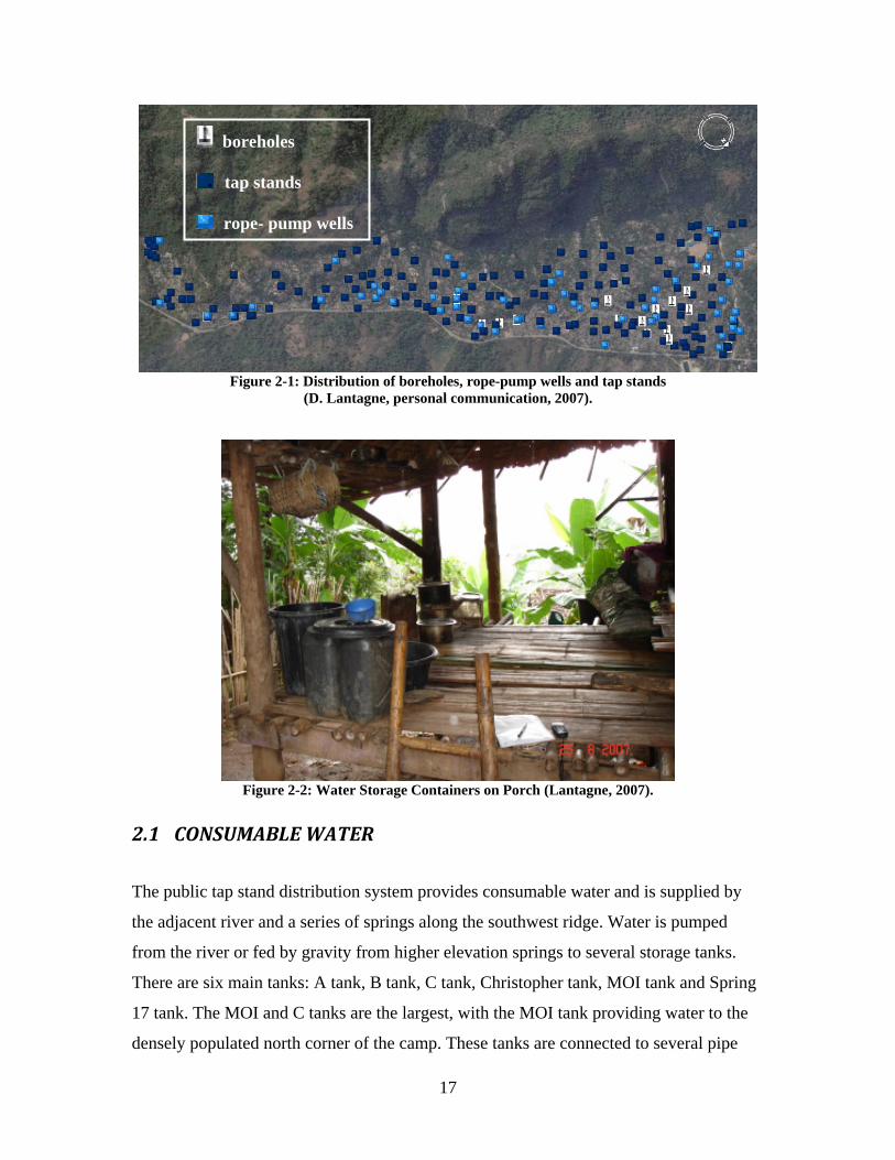
LIST OF FIGURES FIGURE 1-1: AVERAGE MONTHLY RAINFALL FOR MAE SOT, THAILAND (GOSIC, 2007). ............................ 11 FIGURE 1-2: LOCATION OF MAE LA REFUGEE CAMP .................................................................................... 13 FIGURE 1-3: MAE LA LOCATION, LOOKING SOUTHWEST (DATA FROM LANTAGNE, 2007). ........................... 13 FIGURE 1-4: UN REFUGEE CAMP POPULATIONS AND DEMOGRAPHICS (UNHCR, 2006). ............................. 14 FIGURE 2-1: DISTRIBUTION OF BOREHOLES, ROPE-PUMP WELLS AND TAP STANDS ........................................ 17 FIGURE 2-2: WATER STORAGE CONTAINERS ON PORCH (LANTAGNE, 2007). ............................................... 17 FIGURE 2-3: DIVISION OF 2007 FLOW VOLUME FROM STORAGE TANKS BY SOURCE. ................................... 18 FIGURE 2-4: TYPICAL ROPE-PUMP WELL (LANTAGNE, 2007)......................................................................... 20 FIGURE 3-1: SOFTWARE AND APPLICATIONS FOR ARCGIS DESKTOP. .......................................................... 23 FIGURE 3-2: EPANET MODEL OF SECTION OF SPRING 17 IN MAE LA........................................................... 26 FIGURE 4-1: TAP STANDS IN MAE LA CAMP. ................................................................................................ 28 FIGURE 4-2: VISUAL INSPECTION IDENTIFICATION OF HOMES. ..................................................................... 29 FIGURE 4-3: AVERAGE AND STANDARD DEVIATION OF ERROR BETWEEN GEOGRAPHIC POSITIONS
MEASURED BY MIT AND DANIELE LANTAGNE.................................................................................... 31 FIGURE 4-4: ELEVATION ERROR BASED ON DEM INFORMATION AND CORRESPONDING XY ERROR............ 31 FIGURE 4-5: MODIFIED DEM WITH TAP STAND LOCATIONS BY SYSTEM...................................................... 32 FIGURE 5-1: CONSUMPTION AND TRAVEL TIMES (WELL, 1998). ................................................................. 33 FIGURE 5-2: HOME DISTANCE TO NEAREST TAP STAND. .............................................................................. 35 FIGURE 5-3: HOME DISTANCE TO NEAREST TAP STAND - HISTOGRAM......................................................... 36 FIGURE 5-4: HOME DISTANCE TO NEAREST ROPE-PUMP WELL. ................................................................... 38 FIGURE 5-5: HOME DISTANCE TO NEAREST ROPE-PUMP WELL - HISTOGRAM.............................................. 39 FIGURE 5-6: NEAREST ROPE-PUMP WELL AND DEM.................................................................................... 40 FIGURE 5-7: DAILY HOME WATER AVAILABILITY. ....................................................................................... 42 FIGURE 5-8: WATER VOLUME DISTRIBUTION - HISTOGRAM. ........................................................................ 43 FIGURE 7-1: KML2SHP EXPORT SCREEN SHOT. ............................................................................................. 52 FIGURE 7-2: ADDING XY DATA TO ARCMAP AND SETTING COORDINATE SYSTEM...................................... 54 FIGURE 7-3: CONVERTING RASTER TO FEATURES. ........................................................................................ 56
7
LIST OF TABLES TABLE 5-1: TAP STANDS WITH INADEQUATE WATER VOLUME..................................................................... 44 TABLE 6-1: SUMMARY OF HOMES WITH INADEQUATE ACCESS..................................................................... 45 TABLE 6-2: BREAKDOWN AND OVERLAPPING BURDENS FOR HOME WATER ACCESS................................... 46
8
1 INTRODUCTION
A geographic information system (GIS) is a useful tool to understand spatial relationships
and visualize problems in new ways. This work utilizes a GIS in coordination with a
computer model created by Navid Rahimi (2008) to better understand the condition of
water supply within Mae La camp, Thailand. This chapter and the next are collaborative
works from the author, Katherine Vater and Navid Rahimi who worked together as a
project team under the Master of Engineering program in the Department of Civil and
Environmental Engineering at MIT.
Mae La camp is located along the border of Thailand and Myanmar and the features of
this region are reflected within the camp itself. This chapter lays a cultural framework for
the water system within the camp, which is described in detail in Chapter 2.
1.1 THE THAILAND – MYANMAR BORDER
Mae La camp is a refuge for thousands of people seeking protection from persecution in
Myanmar. Ongoing turmoil shapes the lives of the people within the camp.
Understanding the available water resources within the camp requires knowledge of not
only the regional climate and geography, but the reasons people are living in Mae La and
the conditions found there.
1.1.1 Politics
In September 1988 a military junta took control in Burma killing as many as 10,000
people (Lanser, 2006). The military regime has placed restrictions on work and civil
liberties and has become increasingly brutal, especially towards ethnic minorities. As a
result, a large number of people from Myanmar have fled to escape poverty or
persecution. It is estimated that the largest number, about 2 million people, have migrated
into Thailand, although the exact numbers are unknown. Of these, about 140,000 reside
9
in United Nations (UN) sanctioned camps and 500,000 are registered migrant workers.
The rest remain unregistered and attempt to stay unnoticed to avoid being deported back
across the border (Fogarty, 2007).
Wages in Myanmar are not sufficient to meet the basic needs of most families, and so
many workers are forced to look for work outside Myanmar’s borders. Migrants can
apply for legal working papers in Thailand which affords them one (and only one) year of
legal work. With these papers, workers have the best chance of receiving at least the
minimum wage and experiencing decent working conditions. Many Thai business owners
rely on illegal workers for an unending supply of cheap labor. In Mae Sot, the closest city
to the Mae La camp, it is estimated that around 50% of the 80,000 Myanmar people have
papers (McGeown, 2007).
Illegal residents are often forced to pay bribes to Thai authorities to avoid being captured.
When these authorities do take action, the person is forcefully returned to Myanmar. In
most cases of deportation, however, the migrant can often merely pay a small bribe to the
Myanmar border guard and return again to Thailand. In other cases, the Thai authorities
report the migrant to the Myanmar government and heftier governmental fines must be
paid in order to avoid jail time (McGeown, 2007).
Much of the challenge for these migrants stems from the fact that Thailand is not a
signatory of the UN Refugee Convention. Accordingly, the government only grants
asylum to those fleeing combat as opposed to those fleeing human rights violations
(Refugees International, 2007). This makes the situation complicated as the UN-
sanctioned camps along the border are officially called temporary shelters by the Thai
government, while in reality many families have lived in these camps for more than 20
years. It is the intention of the Thai government that the residents either return to
Myanmar or move on and repatriate to another nation. It is illegal, yet common practice,
for camp residents to work in the surrounding Thai towns. They will generally try to find
whatever day labor is available and send money earned back to Myanmar to provide for
remaining family members (D. Lantagne, personal communication, October 19, 2007).
10
Native hill tribes, which historically lived impartially across Northern Thailand and what
is now Myanmar, make up a large majority of the resettling group. The Karen, Karenni,
Shan, and Mon are the main tribes that are being driven from their homes by the
Myanmar military (McGeown, 2007). Within Myanmar there is some resistance from the
Karen National Liberation Army (KNLA) which is fighting for an independent Karen
state. There were additional rebel armies, but over the past 20 years most have agreed to
ceasefires with the military junta. Many of the refugees in the camps in Thailand are
sympathetic to the KNLA, and some have even served in it (McGeown, 2007).
The Karen believe strongly in the value of family. As a result, decisions to leave the
camps and repatriate are difficult and must be made as a family. Generally, the teenagers
and young adults who have lived most of or all of their lives inside the camp want to
repatriate elsewhere while older generations hope to return to Burma if it is restored (D.
Lantagne, personal communication, October 19, 2007).
1.1.2 Economy
As described above, there is a significant amount of poverty in Myanmar as a result of
the military junta’s overbearing controls and inefficient economic policies. Inconsistent
exchange rates and a large national deficit create an overall unstable financial atmosphere
(CBS, 2007). Although difficult to accurately assess, it is estimated that the black market
and border trade could encompass about half of the country’s economy. Importing many
basic commodities is banned by the Myanmar government and exportation requires time
and money (McGeown, 2007). Timber, drugs, gemstones and rice are major imports into
Thailand while fuel and basic consumer goods such as textiles and furniture are exported
(CBS, 2007).
By night, the Moei River, which divides the two countries, is bustling with illicit activity.
Through bribing several officials, those who ford the river are able to earn a modest profit
(for example around 2 USD for a load of furniture) and provide a service to area
merchants and communities. Thailand benefits from a robust gemstone business that
11
draws dealers from all over the world. The Myanmar mine owners would get a fraction of
the profit by dealing directly with the government (McGeown, 2007).
1.1.3 Climate in Northern Thailand
The Tak region of northern Thailand is characterized by a tropical climate with wet and
dry seasons (UN Thailand, 2006; ESS, 2002). The rainy season lasts from June to
October, followed by a cool season until February. The weather turns hot and sunny
between March and May (UN Thailand, 2006). The northern region of Thailand has an
average temperature of 26ºC although there is significant variation over the year due to
the elevation. Typical temperatures range from 4ºC to 42ºC (Thailand Meteorological
Department in ESS, 2002). The average annual rainfall in Mae Sot, Thailand is 2100
millimeters (mm) (GOSIC, 1951-2007), and Figure 1-1 shows the monthly rainfall
averages over the past 56 years. The rainy season is clearly visible, and more than 85% of
the annual 2100 mm falls during this period.
0
20
40
60
80
100
120
140
160
J F M A M J J A S O N D
Month
Mon
thly
Rai
nfal
l [m
m]
Figure 1-1: Average Monthly Rainfall for Mae Sot, Thailand (GOSIC, 2007).
12
1.2 MAE LA CAMP
The Mae La camp is a refuge for people seeking protection from the Myanmar
government and from warfare along the Thailand-Myanmar border (McGeown, 2007).
The camp is run by the United Nations High Commissioner on Refugees and has existed
since 1984 (TBBC, No Date).
1.2.1 Location and Demographics
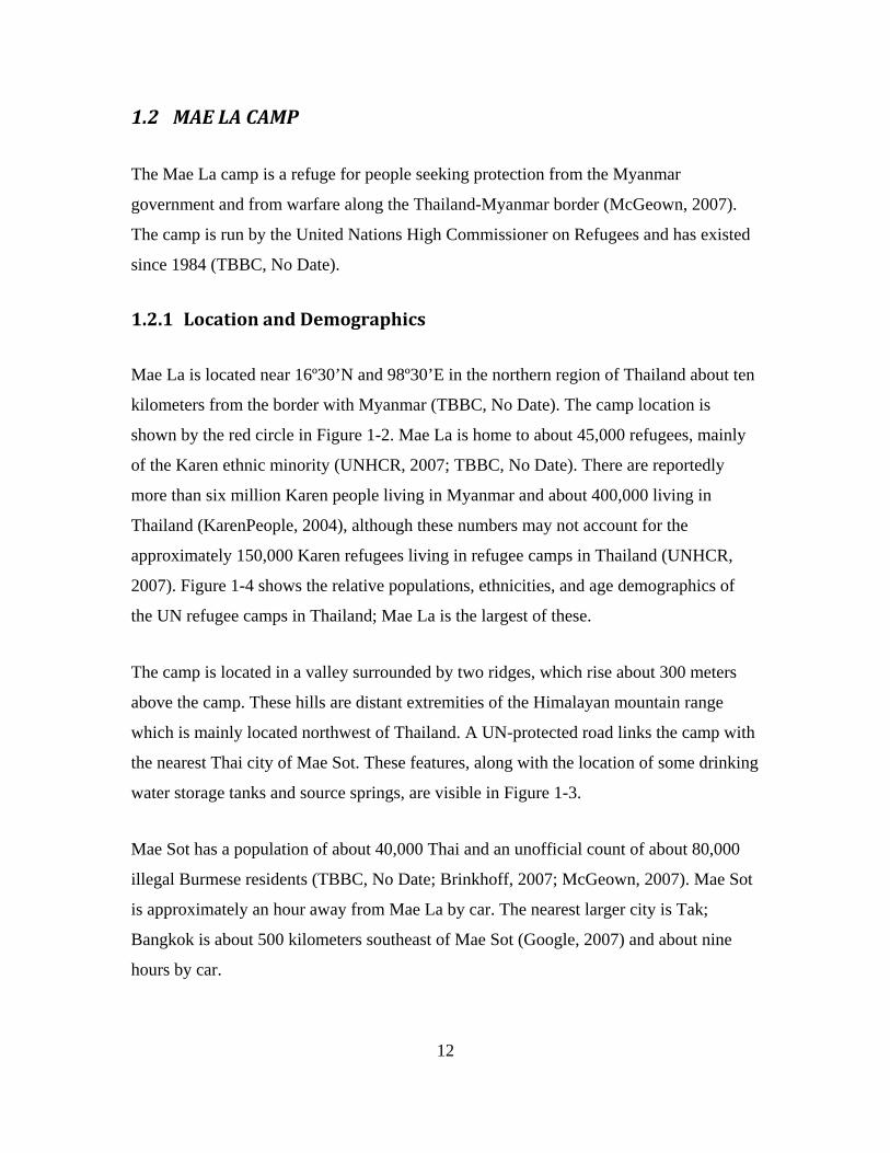
Mae La is located near 16º30’N and 98º30’E in the northern region of Thailand about ten
kilometers from the border with Myanmar (TBBC, No Date). The camp location is
shown by the red circle in Figure 1-2. Mae La is home to about 45,000 refugees, mainly
of the Karen ethnic minority (UNHCR, 2007; TBBC, No Date). There are reportedly
more than six million Karen people living in Myanmar and about 400,000 living in
Thailand (KarenPeople, 2004), although these numbers may not account for the
approximately 150,000 Karen refugees living in refugee camps in Thailand (UNHCR,
2007). Figure 1-4 shows the relative populations, ethnicities, and age demographics of
the UN refugee camps in Thailand; Mae La is the largest of these.
The camp is located in a valley surrounded by two ridges, which rise about 300 meters
above the camp. These hills are distant extremities of the Himalayan mountain range
which is mainly located northwest of Thailand. A UN-protected road links the camp with
the nearest Thai city of Mae Sot. These features, along with the location of some drinking
water storage tanks and source springs, are visible in Figure 1-3.
Mae Sot has a population of about 40,000 Thai and an unofficial count of about 80,000
illegal Burmese residents (TBBC, No Date; Brinkhoff, 2007; McGeown, 2007). Mae Sot
is approximately an hour away from Mae La by car. The nearest larger city is Tak;
Bangkok is about 500 kilometers southeast of Mae Sot (Google, 2007) and about nine
2. ArcEditor – All ArcView properties along with scan digitization, enhanced database editing capabilities, and more
3. ArcInfo – All ArcEditor properties along with advanced cartography and more geoprocessing tools
Useful Applications: (all software levels)
ArcMap ArcToolbox• Main Application
• Map based tasks
• Collection of geoprocessing tools
•Ex: spatial anaylstmakes contours
ArcCatalog• Organize and manage geographic info incl.: data, maps, tools, metadata
Figure 3-1: Software and Applications for ArcGIS Desktop.
24
Unlike Google Earth discussed below, ArGIS software is not free and requires licensing.
Additionally, given the wide range of features and capabilities, this program is not
intuitive and does take some familiarization in order to use effectively. There is an
extensive amount of training and support including forums and script downloads
available on the main ESRI website. In addition, Appendix A contains useful information
on the ways ArcGIS was utilized for this project.
3.4 GOOGLE EARTH
Google Earth has been gaining popularity as a way of displaying and manipulating
geographic information. A major draw of the product is the fact that it is free and
available for download through http://earth.google.com. While additional, more advanced
products are available for purchase (Google Earth Plus and Google Earth Pro), for the
scope of this project the standard program was sufficient.
Google Earth utilizes Keyhole Markup Language (KML) files which are used for
defining a set of geographic information features such as points and images in two or
three dimensions (Google Earth, 2007). The KML file can be grouped (zipped) with icon
and/or overlay images as a cohesive KMZ file.
New point, shape, and image overlay files can be created by selecting options from the
Add menu. The nomenclature changes slightly from ArcView (“Point” becomes
“Placemark”, “Polyline” become “Path”, etc.) but the general functions remain the same.
3.5 DIGITAL ELEVATION MODELS
A digital elevation model (DEM) is a representation of the ground surface elevation.
Most commonly a raster, or grid of squares, is used to section an area and each grid is
assigned an elevation. A distance modifier associated with a DEM refers to the precision
of the data. For example, a thirty-meter DEM would have a grid size of thirty by thirty
meters. The smaller the grid size, the more precise and detailed the data.
25
3.6 EPANET
This section is the result of collaboration between the author and Navid Rahimi.
EPANET is a computer program that simulates hydraulic and water quality behavior
within pressurized pipe networks. It was developed by the United States Environmental
Protection Agency (EPA) and presents the great advantage of being available on the
internet free of charge. It can model networks of pipes, nodes, pumps, valves and storage
tanks or reservoirs and tracks the flow of water in each pipe, the pressure at each node,
the height of water in each tank, and the concentration of a chemical in the network
during a time stepped simulation.
Some of the key hydraulic capabilities of EPANET include no size limitations on the
network, handling multiple head-loss equations, simulating time-varying demand, and
pump operation control (e.g. based on tank water levels). No model can perfectly reflect
the underlying system but these capabilities enhance the realism of the simulation
(Rossman, 2000).
One important scenario that is not built into the EPANET software is the intermittent
flow case which is relevant for Mae La as well as many developing countries or
situations of crisis. It is possible to vary the demand or supply of the system with time,
but EPANET assumes a constantly pressurized system, with full pipes at the start of the
period.
The model results are easily exported from EPANET for further analysis in coordination
with geographic home location. Modeled flow rates and pressures can be viewed in the
GIS interface.
26
Figure 3-2 illustrates a sample EPANET model output from a section of the Spring 17
system. Variations in flow rates are shown through different colored pipes, while pressure
is depicted as a number and color at each node (tank, tap stand, or valve). For this
sample, all of the pressures are less than 25 meters and depicted in dark blue.
Figure 3-2: EPANET model of Section of Spring 17 in Mae La.
27
4 DATA COLLECTION & ANALYSIS
I used several different data sources for this work. Before a site visit to the Mae La camp,
significant Global Positioning System (GPS) data was received from Daniele Lantagne
and some pipe network specifications from Joel Terville, the Logistics Coordinator for
the Mae La camp through AMI. The site visit consisted of going to a large portion of the
tap stands related to the major tanks as well as measuring pipe lengths and recording
diameters. Additionally, Dr. Bunlur Emaruchi from the Faculty of Civil Engineering of
Mahidol University in Bangkok supplied a DEM which was received during the site visit.
Upon return to Cambridge, home location data was collected through inspection of
Google Earth images.
4.1 ONSITE COLLECTION
While on-site, more than 130 of the 152 tap stands were visited and referenced using a
Garmin eTrex Vista handheld GPS device. Figure 4-1 shows the location of all the tap
stands in the camp (D. Lantagne, personal communication, 2007) noting which were
visited in January 2008. The pipe network specification data (e.g. distance between nodes
in the system) was checked using a laser range finder. Diameters were confirmed through
visual inspection. The previously supplied data was found to be largely inaccurate. Most
of the general layout of the pipe system and connections portrayed was the same as found
in the field, but the distances we measured were very different than those supplied. In one
case, a pipe length was recorded as being around 90 meters and our measurements
resulted in twice that value. As a result, the AMI-supplied data is not used in this work
even though it does contain information for parts of the network that we did not visit.
28
Figure 4-1: Tap Stands in Mae La Camp.
4.2 HOME LOCATION DATA
Homes were identified through visual inspection using Google Earth, and in the first
attempt, 6,704 homes were found. Buildings that were obviously not homes like the
hospital and NGO offices were not included in the set. In Figure 4-2, the large,
rectangular building with the blue roof in the upper right section is not selected as a
home.
According to Frédéric Pascal (personal communication, April 21, 2008) it is estimated
that the actual number of homes in the camp is between 8,500 and 9,000. A more careful
examination of the camp was completed while being less discriminating about potential
homes in areas where the picture was not entirely clear. A final number of 7,117 homes
were found and the discrepancy between this number and the likely actual number of
homes can be attributed to vegetation cover and to the precision of the aerial
photographs.
Since the highly populated areas, such as in the northeast section of camp, have sparse
vegetation cover, it is likely that more homes were unidentified in the less populated
areas. This may affect the results since the less populated areas also tend to be further
away from infrastructure points of interest such as tap stands and rope pump wells. It is
thus possible that the results are skewed so that a fewer number of homes, both as a
percentage and a raw number, are identified as being undesirably far from water points.
N
29
Figure 4-2: Visual Inspection Identification of Homes.
4.3 ELEVATION DATA
Elevation was measured with the built-in barometric, or pressure, altimeter in the
handheld GPS. However, atmospheric pressure varies from day to day, introducing error
into the altimeter readings. Differences in elevation measurements at the same point were
found to be upwards of forty meters. We recorded the time of each measurement and took
several measurements at a reference point throughout the day. We adjusted each
measurement assuming that the elevation change was linear between reference point data.
After taking the overall average elevation for the reference point over the three weeks, we
adjusted all other measurements to this benchmark based on the measured reference-point
elevations before and after the measurement.
For example, suppose a benchmark for the reference value was decided to be 175 meters
or the average value throughout the site visit. On one particular day suppose we measured
elevations of 185 meters at noon and 195 meters at 4PM. Between noon and 4PM we
made measurements at other points. Suppose we measured an elevation of 250 meters at
2PM. Based on our prior and subsequent measurements of the reference point, we would
interpolate the reference value to be 190 meters at 2PM. Since this is 15 meters higher
Non-
home
Heavy
Vegetation
30
than the benchmark elevation of 175 m, we would subtract 15 meters from the elevation
measured at 2PM to arrive at a corrected elevation of 250 – 15 = 235 meters. While this
does account for some of the local variation in pressure, we were not very comfortable
with the linear assumption and with the overall degree of change.
As an alternative to the altimeter readings, a two-meter DEM was received for the entire
camp area (B. Emaruchi, personal communication, March 26, 2008). By definition, a
two-meter DEM defines areas of four square meters as having a single elevation but
variations within those grids remain hidden. This DEM reports elevations to the nearest
meter. Error in the latitudinal and longitudinal locations of our points along with variation
within the four square meters determines the accuracy of the elevation data using a DEM.
Product specifications for the eTrex Vista state that the device is accurate to within 15
meters horizontally 95% of the time (Garmin, 2008).
By comparing the latitude and longitude measured in January 2008 with the already
available infrastructure point locations from Daniele Lantagne, we were able to get a
concrete sense of these errors. The differences are grouped by tap stands associated with
the various tanks (A, B, Spring 6/7, etc.) within the distribution system. The average error
is shown as a triangle in Figure 4-3 with the vertical bars representing the standard
deviation. It is important to note that this XY error is not with respect to a known actual
datum but rather two measurements taken, about five months apart, with different
equipment.
Using the DEM we were able to ascertain an average and standard deviation of elevation
error associated with changes in XY position. The average XY measurement differences
found correspond to changes in altitude of around three meters as shown in Figure 4-4.
Examining the DEM in areas near the start of the steep mountain ridge along the
southwest border of the camp, however, differences in 15 meters in XY location can be
associated with changes of elevation as high as 10 to 15 meters.
31
0
2
4
6
8
10
12
14
16
18
20
A B C CH MOI S 6/7 S 8 S 17
S ystem
XY Error (m
eters)
Figure 4-3: Average and Standard Deviation of Error Between Geographic Positions Measured by
MIT and Daniele Lantagne.
‐2
0
2
4
6
8
A B C CH MOI S 6/7 S 8 S 17
S ystem
Eleva
tion Error (m
eters)
Figure 4-4: Elevation Error Based on DEM Information and Corresponding XY Error.
Most of the tap stands are located in the lower lying regions of the camp with less drastic
elevation change, but the tanks and certain systems are closer to the ridge and thus the
same errors in XY location create more drastic errors in the associated elevation. From
Figure 4-5, the large MOI system is not as much a concern for elevation error as the A
system. The cluster of taps in the Spring 17 (S17) system located in the upper left of the
figure represents the secluded tuberculosis quarantine village (TB) which was not
included in the EPANET model.
32
System
Figure 4-5: Modified DEM with Tap Stand Locations by System.
Elevation (meters)
N
33
5 RESULTS
Through the analysis of home, tap stand, and rope-pump well locations along with
outputs from the EPANET model, the effectiveness of water access within Mae La camp
is accessed. This chapter identifies homes and regions with inadequate service concerning
one or more of the following:
1. Location at a distance to tap stand that impacts consumption 2. Location at a distance to rope-pump well that impacts consumption 3. Insufficient daily water volume availability
5.1 TAP STAND PROXIMITY
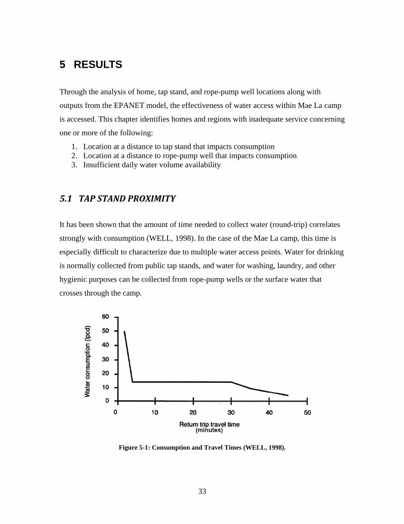
It has been shown that the amount of time needed to collect water (round-trip) correlates
strongly with consumption (WELL, 1998). In the case of the Mae La camp, this time is
especially difficult to characterize due to multiple water access points. Water for drinking
is normally collected from public tap stands, and water for washing, laundry, and other
hygienic purposes can be collected from rope-pump wells or the surface water that
crosses through the camp.
Figure 5-1: Consumption and Travel Times (WELL, 1998).
34
While most families gather drinking water from the public tap stands, others have direct
connection within their homes. When the camp logistic team discovers unauthorized
connections, they confiscate the pipes and communicate with owners about proper use of
the public system. These connections are obviously unknown and therefore not accounted
for in the analysis. Connections that take overflow water from springs by placing a pipe
downstream of the system intake point are permitted although only utilized by a small
percentage of the camp. Tracking homes with these connections is beyond the scope of
this project, and authorized private connections are therefore not considered. This
analysis also assumes that each home gathers drinking water from the nearest public tap
stand.
As shown in Figure 5-1, when the return-trip travel time to source water is less than about
three minutes, water consumption drastically increases. Tap stands should be located at a
distance that will take the water carrier 1.5 minutes to travel. The range of comfortable
walking pace considered was 75-85 meters per minute (Bohannon, 1997). It is customary
in the camp for the strongest population group, young men, to fetch water for the
household. Children carrying water is discouraged in part by AMI’s practice of
intentionally breaking tap handles which makes them more difficult to operate with small
hands. Even though a healthy and presumably fast walking group fetches the water, a
conservative walking speed of 75 meters per minute is used. Additionally, the topography
of the camp adds to walking difficulty and a large quantity of water must be carried for
half the journey making the lower end of this range more suitable. Assuming this speed
and that each home should be within a 1.5 minute walk, the maximum allowable tap
stand distance is 115 meters.
Figure 5-2 shows an overall view of the camp with homes represented by different colors
based on distance to the nearest viable tap stand. Tap stands are considered viable if
public drinking water is provided for collection. For example, public latrines and private
taps for NGOs are not included.
35
Distance (meters)
Tap Stands
Figure 5-2: Home Distance to Nearest Tap Stand.
N Low Coverage
Region
Spring 2 Region
36
There are 349 of the 7,117 homes identified (less than 5%) located further than 115
meters from the nearest viable tap stand. Many of the homes of concern (in red) are
located in the upper right corner of Figure 5-2 near the Spring 2 system. This region of
the camp happens to be very well supplied by natural springs and the population tends to
acquire water from outside the distribution network (Terville, personal communication,
January 2008). For this reason, the calculated distance to a viable drinking water source is
likely inflated.
Only 210 or less than 3% of homes lie outside a 115 meter distance to a public drinking
water source when these Spring 2 homes are not considered. Fifty percent of homes are
located between 30 and 60 meters from a drinking water source. Figure 5-3, a histogram
of the results, includes the Spring 2 homes. When these homes are not included, the
number of homes with tap stands located more than 200 meters away is reduced by 60%.
Figure 5-3: Home Distance to Nearest Tap Stand - Histogram.
From Figure 5-2, we see a large cluster of homes of concern located between the Spring
17 and A systems (“Low Coverage Region”) in addition to the Spring 2 region. Besides
these two major regions, homes of concern are sparingly distributed mostly along the
mountain ridge that runs along the camp border furthest from the access road. Placing
taps along this ridge is difficult as the slope becomes very steep and many of the homes
37
are located at higher elevations than the system storage tanks. Since the systems are run
by gravity, it is impossible to supply tap stands at these elevations.
Improvement appears possible for the “Low Coverage Region” highlighted in Figure 5-2.
This is a large cluster of homes and the elevations are not prohibitively high in
comparison to the A and Spring 17 tanks.
5.2 ROPEPUMP WELL PROXIMITY
It is also important to have access to hygienic water for laundry, bathing, and hand
washing, which does not need to be disinfected through chlorination. For this, residents
do not use the twice-daily distributed water, but rather one of the 61 working rope-pump
wells or surface water that cuts through the camp. During most of the year these surface
water sources are plentiful, but deep in the dry season will often run low or dry (Terville,
personal communication, January 2008).
It is customary for people to bathe at the rope-pump wells and bring their laundry to the
well to wash near the water. This way, large amounts of water do not need to be carried
back to the home and use mainly occurs at the well. Since use is at the source, the “return
trip” time is not as relevant as with the consumable water. This would make it reasonable
to set the distance for concern limit at twice that for the tap stands. There is a
disadvantage of each member of the home needing to walk to the well as opposed to one
person who can bring consumable water for all back to the home. Also, a moderate to
small amount of water is carried to the homes from the wells for at-home hand washing,
dish washing, in-home latrines, and for those who cannot or will not bathe at the rope-
pump wells (e.g. sick and elderly). Heavy, wet laundry must also be carried back from
the wells. Since much of the water use occurs at the rope-pump well but some at the
home, the critical distance limit is set at 180 meters or approximately one and a half times
the critical tap stand distance. This criterion is used in Figure 5-4 to identify homes that
are problematically distant from a rope-pump.
38
Distance (meters) Rope-Pump Wells
Figure 5-4: Home Distance to Nearest Rope-Pump Well.
N
39
Under this criterion, just over 1000 homes, or 14%, are an unreasonable distance from the
nearest rope-pump well (Figure 5-5). Over one half of the homes have a rope-pump well
somewhere between 30 and 100 meters away. There is a much greater number of homes
located far from rope-pump wells, but this may not be easily remedied and there are
additional sources of washing water. Also, there is a stream that runs west through the
camp to the river in the northwest which can act as an alternative supply. While many of
the homes in red are along the mountain ridge at the top of the Figure 5-4 are far from the
river and stream, these sources do afford some homes a closer water source than the
wells.
Figure 5-5: Home Distance to Nearest Rope-Pump Well - Histogram.
It is likely that drilling wells along the mountain ridge is not economically feasible given
the greater depth to the water table from the increased elevations. Since a rope-pump well
relies on the ability of the user to pull water from the water table to the surface, the wells
are ill suited for locations where this distance is large. The areas of concern correlate with
the high regions of the DEM. Figure 5-6 shows that many of the homes in red are located
in the highest elevation zones within the camp.
40
Distance (meters) Rope-Pump Wells
Elevation (meters)
Figure 5-6: Nearest Rope-Pump Well and DEM.
N
41
5.3 VOLUME OF WATER PER HOUSEHOLD
Through linking the results of Navid Rahimi’s EPANET model (Rahimi, 2008) with
home locations, an estimate of available water volume per home is made. Rahimi’s
model predicts the average flow rate for 102 of the 139 viable tap stands. He shows that
flow rates are very nearly constant throughout the six hours of operation and tanks do not
run dry with normal use. Therefore, flow rates can be multiplied by distribution time to
find daily available volume.
A conservative estimate for a minimum amount of consumable water is 7.5 liters per day
per capita (UNDP, 2006). This includes about two liters per day for drinking and the
remainder for food preparation. Since residents in Mae La camp use tap stand water for
consumption only, this is an appropriate number for an analysis of tap stand water
volume.
We use homes as a proxy for population. While this is not a perfect fit since some homes
or regions of camp may be more densely populated than others, when looking at a broad
view of the entire camp it should be a suitable approximation. Assuming an even
distribution of a population of 45,000 among an estimated 8,500 homes, there would be
between five and six people per home (F. Pascal, personal communication, April 21,
2008). Thus, 50 liters per home per day is a conservative estimate for the minimum
amount of consumable water.
Some of the small spring systems were not included in the EPANET model which
accounts for only 102 available predicted flow rates. Of the over 7,000 homes visually
identified, 5,500 are included in the volume analysis. These are the homes whose closest
viable tap stand is one of the 102 included in the model.
For each home, daily flow volume for the nearest tap stand was divided by the total
number of homes associated with that tap stand. The distribution of daily availability of
drinking water per home and shown in Figure 5-7.
42
Water Available per Home (liters/day)
Viable Tap Stands
Figure 5-7: Daily Home Water Availability.
N
43
The homes of concern, shown in red and orange, are scattered throughout the camp.
There is no single subsystem within the overall network where flow is low and no
geographic similarities between the homes of concern, such as being located along the
steep mountain ridge. Homes for which the closest viable tap stand was not included in
the EPANET model are shown in black.
Figure 5-8: Water Volume Distribution - Histogram.
A total of 809 homes, or 15% of those considered, are categorized as unable to obtain 50
liters of water per day (Figure 5-8). By tracing these underserviced homes back to the
originating taps, we find that there are 15 tap stands of concern.
There is definitely error in the model results because the model predicts flow rates of zero
liters per minute at nine of the tap stands. Flow was observed at these tap stands during
the site visit, however. It is most likely that these errors are related to the elevation
assigned to the tap stands based on the GPS location. As discussed in Section 4.3, the
GPS location error can create significant error in elevation. Since the model is driven in
large part by these elevation differences, the model results are sensitive to these errors
(Rahimi, 2008). Excluding the nine tap stands with zero flow, 365 homes, or 7%, are
unable to collect sufficient water volume.
44
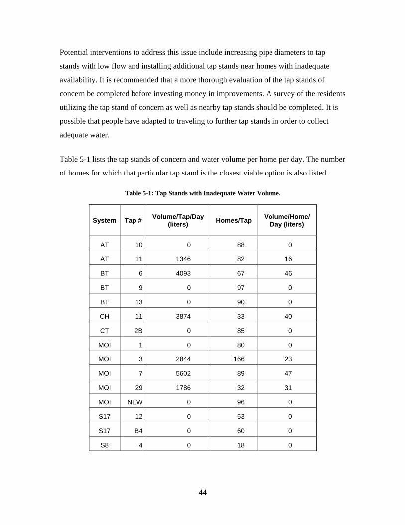
Potential interventions to address this issue include increasing pipe diameters to tap
stands with low flow and installing additional tap stands near homes with inadequate
availability. It is recommended that a more thorough evaluation of the tap stands of
concern be completed before investing money in improvements. A survey of the residents
utilizing the tap stand of concern as well as nearby tap stands should be completed. It is
possible that people have adapted to traveling to further tap stands in order to collect
adequate water.
Table 5-1 lists the tap stands of concern and water volume per home per day. The number
of homes for which that particular tap stand is the closest viable option is also listed.
Table 5-1: Tap Stands with Inadequate Water Volume.
System Tap # Volume/Tap/Day (liters) Homes/Tap Volume/Home/
Day (liters)
AT 10 0 88 0
AT 11 1346 82 16
BT 6 4093 67 46
BT 9 0 97 0
BT 13 0 90 0
CH 11 3874 33 40
CT 2B 0 85 0
MOI 1 0 80 0
MOI 3 2844 166 23
MOI 7 5602 89 47
MOI 29 1786 32 31
MOI NEW 0 96 0
S17 12 0 53 0
S17 B4 0 60 0
S8 4 0 18 0
45
6 CONCLUSION AND RECOMMENDATIONS
Overall this research shows that the vast majority of residents in Mae La have sufficient
access to water. A water use survey is recommended in order to verify the findings of this
research and modify the GIS tool for future work. The assumptions that every home
utilizes the rope-pump well or tap stand that is of closest proximity may or may not be
valid. A major area of concern, especially regarding the EPANET model results, is in
attaining accurate locations and especially elevations of tap stands and water
infrastructure points within the camp.
6.1 OVERALL WATER ACCESS
This research used GIS to assess three major indicators—home distance to tap stands,
home distance to rope-pump wells, and volume of drinking water per home—with results
summarized in Table 6-1. The overall results show that the access issue of least concern
is proximity to public tap stands.
Table 6-1: Summary of Homes with Inadequate Access.
Homes with Far Taps* 349 (5% of 7,117) Homes with Far Rope-Pump Wells 1,017 (14% of 7,117) Homes with Low Volume 809 (15% of 5,500) *Reduces to 210 (3%) when not including Spring 2 region
There are homes that fail more than one test, however. Table 6-2 shows a breakdown of
the results considering that some homes will have multiple problems. Of homes
identified, 73% are adequately serviced. Roughly one fifth of these homes are located
nearest to tap stands not included in the EPANET model and therefore the volume test
was not completed.
46
Table 6-2: Breakdown and Overlapping Burdens for Home Water Access.
Flow Data No Flow Data Total Far Tap, Far Well & Low Volume 18 - 18 Far Tap & Low Volume 18 - 18 Far Well & Low Volume 52 - 52 Far Tap & Far Well 78 93 171 Far Tap Only 37 105 142 Far Well Only 471 305 776 Low Volume Only 721 - 721 Near Tap, Near Well & High Volume 4,105 1,114 5,219 Total 5,500 1,617 7,117
6.2 POTENTIAL IMPROVEMENTS
There are a variety of concerns regarding these results and what service is actually
provided in the camp. As mentioned in Section 5.2, the proximity to the nearest rope-
pump well may not relate directly to water use since there are additional sources for non-
drinking water such as bore holes and surface water. A water use survey that gathers
information from a variety of homes dispersed throughout the camp would help better
understand the extent of these alternative sources. The survey should account for seasonal
change either by clearly asking questions about the different season or by surveying at
multiple points throughout the year.
This survey could strive to understand how different groups, based on geography, wealth,
ethnicity, gender, or age, access and utilize water. While logically homes located in the
very steep sections of camp far from a public tap may adapt to using less water, there
may be other subtle differences about the use of bore holes based on age or gender. The
survey should ask which tap stands are frequented by the home. Do different members of
47
the home prefer different tap stands and what are the perceived benefits? It was observed
during the field visit that some systems (B System, for one) had perceivably higher
pressures which resulted in shorter lines at the tap stands. How much further is a person
willing to walk in order to avoid waiting for water?
A major improvement to the existing GIS information would be to obtain more accurate
elevation and XY-location information for infrastructure points. This would help create a
more accurate EPANET model which in turn produces the flow results that are viewed
through the GIS program. There is a significant portion of the underserviced homes
attributable to tap stands for which the model predicts flows of zero liters per day, when
in fact water was observed at these stands. These and perhaps other erroneous
predictions are the result of errors in measuring the elevation of water system
components.
48
References
Aide Médicale Internationale (AMI). (2007). Mae La Distribution Data. Unpublished distribution data. Thailand: Aide Medicale Internationale.
Aide Médicale Internationale (AMI). (2007). Missions: Thailand. Retrieved December
12, 2007 from http://www.amifrance.org/-Thailand-.html ArcUser. (2008). Datums and the UTM Projection. Environmental Systems Research
Institute. Retrieved April 10, 2008, from http://www.esri.com/news/arcuser/0499/utm.html
Bohannon, R.W. (1997). Comfortable and maximum walking speed of adults aged 20-79
years: reference values and determinants. Oxford University Press. Age Ageing. 26:1:15.
Brizou, J. (2006). Thailand Mission: Maela Camp Nov. 2005- Aug. 2006: Final Report.
Unpublished report. Aide Médicale Internationale. Paris, FRANCE. Brinkhoff, T. (2007). City Population: Thailand. Retrieved October 12, 2007, from
http://www.citypopulation.de/Thailand.html CBS Interactive Inc (CBS). (2007). Country Fast Facts: Burma. Retrieved December 16,
2007 from http://www.cbsnews.com/stories/2007/10/04/country_facts.shtml Environmental Software and Services (ESS). (2002). Macro-scale, Multi-temporal Land
Cover Assessment and Monitoring of Thailand. Retrieved October 12, 2007, from http://www.ess.co.at/GAIA/CASES/TAI/chp1to3.html
ESRI. (2006). ArcGIS 9: What is ArcGIS 9.2? Retrieved March 14, 2008 from
Fogarty, P. (2007, October 10). Poverty driving Burmese workers east. BBC News.
Retrieved December 12, 2007, from http://news.bbc.co.uk/go/pr/fr/-/2/hi/asia-pacific/70336633.stm
Garmin. eTrex Detailed Specifications REV0105. Retrieved March 20, 2008 from
https://buy.garmin.com/shop/store/assets/pdfs/specs/etrex_series_spec.pdf Global Observing Systems Information Center (GOSIC). (2007). Global Historic
Climatology Network Daily – Mae Sot, Thailand. Retrieved November 26, 2007, from http://gosic.org/gcos/GSN/gsndatamatrix.htm
Google. (2007). Google maps – Mae Sot, Tak, Thailand. Retrieved October 12, 2007,
from http://maps.google.com
49
Google Earth. (2007). Google Earth User Guide Version 4.2. Retrieved April 9, 2008
from http://earth.google.com/userguide/v4/ug_toc.html KarenPeople. (2004). Who Are The Karen? Retrieved December 5, 2007, from
http://www.karenpeople.org Lantagne, D. (2007). Water and Sanitation Assessment to Inform Case-Control Study of
Cholera Outbreak in Mae La Refugee Camp, Thailand. Unpublished presentation. Centers for Disease Control and Prevention, Atlanta, USA.
Lasner, T. (2006). A Brief History of Burma. UC Berkley School of Journalism.
Retrieved December 17, 2007, from http://journalism.berkeley.edu/projects/burma/history.html
McGeown, K. (2007). Life on the Burma-Thai border. BBC News. Retrieved December
8, 2007, from http://news.bbc.co.uk/2/hi/asia-pacific/6397243.stm National Geodetic Survey (NGS). (2007). Frequently Asked Questions about he National
Geodetic Survey. Retrieved April 10, 2008 from http://www.ngs.noaa.gov/faq.shtml#WGS84
National Oceanic and Atmospheric Administration (NOAA). (2008). Universal
Transvers Mercator Coordinates. Retrieved April 18, 2008 from http://www.ngs.noaa.gov/TOOLS/utm.html.
Polprasert, C., Bergado, D., Koottatep, T., & Tawatchai, T. (2006, Auguest 15). Report
on Water and Environmental Sanitations Assessment of Mae La Temporary Shelter, Thasogyant District, Tak Province, Thailand. Asian Institute of Technology (AIT).
Rahimi, N. 2008. “Modeling and Mapping of MaeLa Refugee Camp Water Supply.”
Master of Engineering Thesis, Massachusetts Institute of Technology, Cambridge, MA, USA.
Refugees International. (2007). Thailand: Humanitarian Situation. Retrieved December
15, 2007 from http://www.refugeesinternational.org/content/country/detail/2894/ Rossman, L.A. (2000). EPANET2 USERS MANUAL. Cincinnati, OH, USA: National
Risk Management Research Laboratory. Available at: http://www.epa.gov/nrmrl/wswrd/dw/epanet.html
Thailand Burma Border Consortium (TBBC). (No Date). Mae Sot area. Retrieved
December 5, 2007, from http://www.tbbc.org/camps/mst.htm
50
United Nations Development Programme (UNDP). (2006). Human Development Report: Beyond Scarcity: Power, poverty and the global water crisis. New York: Palgrave Macmillan.
United Nations High Commisioner on Refugees (UNHCR). (2006, September 20).
Myanmar Thailand border Age distribution of refugee population. Retrieved December 5, 2007, from http://www.unhcr.org/publ/PUBL/3f7a9a2c4.pdf
UNHCR. (2007, May 27). Resettlement of Myanmar refugees under way from northern
Thai camp. Retrieved December 5, 2007, from http://www.unhcr.org/news/NEWS/465430f04.html
UN Thailand. (2006). Thailand Info. Retrieved October 12, 2007, from
http://www.un.or.th/thailand/geography.html Water and Envrionmental Health at London and Loughborough (WELL). (1998).
Guidance manual on water supply and sanitation programmes, WEDC, Loughborough, UK.
51
APPENDIX A: DATA TRANSFER
There were a variety of data types and software used throughout this research. The
existing data received from Daniele Lantagne and our determination of home locations
are Google Earth compatible files. Geographic locations collected using the handheld
GPS was compiled using Microsoft Excel. Excel was also used as an intermediary
program to move data between Google Earth and ArcView 9.2. This Appendix describes
how information was transferred between programs with various data types and is
included to facilitate any future use and modification of the dataset by AMI and
Soldarités.
A.1 CREATING FILES WITH GOOGLE EARTH
Using Google Earth, new points can be added to a map by selecting "New Placemark"
from the "Insert" menu or simply typing Control+Shift+P. The placemark was moved
onto the center of a home's roof and all home points were saved in one folder. Zooming
in and out using the scroll button on the mouse was helpful for getting a better sense of
home boundaries. Also, it was helpful to change the tilt which gave the camp a three-
dimensional look and made some houses more visible. This can be done either by moving
the tilt bar which is located above the compass rose in the upper right of the screen or by
holding Control and using the scroll button. Additionally, by clicking on the compass
rose the orientation of the view can be changed.
A.2 KML AND SHAPEFILE CONVERSIONS
Using shape and KML files interchangeably was important for this project in order to use
the analysis capabilities of ArcGIS and the high quality aerial photos available on Google
Earth.
To work with the Google Earth-created homes file in ArcView, a necessary step was to
convert the Google Earth KML file into a shapefile. The most efficient means of
conversion found was to use a freeware program called “Kml2shape” available at
52
http://www.zonums.com/kml2shp_down.html. Once downloaded the program is simple
to use. After selecting the “Open KML” button and choosing the file, select “Export
SHP”. The datum is then specified as WGS84 and UTM coordinates selected along with
the proper zone for Mae La camp (47 North). Finally, select an output file name and click
“Accept”.
This new shape file can then be opened with ArcMap.
Figure A-1: Kml2shp Export Screen Shot.
A.3 FROM HANDHELD GPS TO COMPUTER
For location data taken on site with the Garmin eTrex Vista, a free program by the
Minnesota Department of Natural Resources, DNR Garmin, was used to transfer all
latitude, longitude and point name data onto the computer. After setting and opening the
appropriate port (e.g. USB) from the GPS menu, “Waypoints” or point data can be
uploaded to the program’s data sheet. At this stage data can be easily manipulated either
in DNR Garmin or can be opened through Excel after saving as a tab delimited text file.
Empty columns and extraneous information is removed, while information such as the
53
number of taps per stand and the type of tap (e.g. latrine, private office source, public tap
stand) is added.
The elevation data from the built-in altimeter and time and date information could not be
automatically taken using the eTrex Vista GPS with DNR Garmin software. A DEM of
the area, created by Dr. Bunlur Emaruchi became the source of our elevation data, and it
was unnecessary to add the altimeter information.
Once the data was cleaned and columns added for tap stand information and type, the file
was saved as a text file that could be opened with ArcMap. One particularly tedious
feature of ArcMap is that the title fields of all data columns cannot contain spaces and
can only begin with a letter. For example, “X_Coord” was a typical name designation.
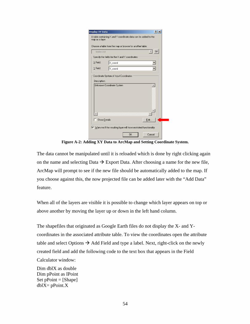
A.4 ADDING DATA TO ARCMAP
Once a shapefile or text file is created, it could be included in the ArcMap view of the
camp. After selecting “Add Data” the file appears as a layer in the bar on the left hand
side of the screen. By right clicking on the layer and selecting “Display XY data” the
proper column headings for the latitudinal and longitudinal coordinates can be selected.
The matching coordinate system can be linked to the data within ArcMap by selecting
“Edit” near the bottom of the prompt screen and navigating through Select Projected
Coordinates UTM WGS84 and finally selecting the file with 47 North zone.
54
Figure A-2: Adding XY Data to ArcMap and Setting Coordinate System.
The data cannot be manipulated until it is reloaded which is done by right clicking again
on the name and selecting Data Export Data. After choosing a name for the new file,
ArcMap will prompt to see if the new file should be automatically added to the map. If
you choose against this, the now projected file can be added later with the “Add Data”
feature.
When all of the layers are visible it is possible to change which layer appears on top or
above another by moving the layer up or down in the left hand column.
The shapefiles that originated as Google Earth files do not display the X- and Y-
coordinates in the associated attribute table. To view the coordinates open the attribute
table and select Options Add Field and type a label. Next, right-click on the newly
created field and add the following code to the text box that appears in the Field
Calculator window:
Dim dblX as double Dim pPoint as IPoint Set pPoint = [Shape] dblX= pPoint.X
55
The last input box in the field calculator window appears underneath a display of the new
field label and an equal sign. Type dblX here. Replace all the “X”s in the above steps to
show the Y-coordinate values.
A.5 ARCMAP ANALYSIS
Once information was added to ArcMap, further analysis could be completed. The
following is a summary of important information:
1. DEM (Dr. Bunlur), 2. Major water system infrastructure location (D. Lantagne) 3. Additional tap stand position (collected during site visit in January 2008) 4. Home locations (Google Earth, visual identification) 5. EPANET model flow rates
A.5.1 Joining Elevation Data
The elevation of infrastructure points withing the system could be assigned using the XY
location and DEM. These elevation were necessary inputs to the EPANET model by
Rahimi (2008) so pressures and flows could be calculated. To link the location and
elevation infromation, the DEM must first be exported as a raster (right click on the layer
and select Export Data). An “Export Raster Data” prompt box appears displaying the
name of the selected layer. Next, the imbedded elevation information, which is displayed
through varying colors, must be converted to an explicit number.
Within the Spatial Analyst extension, which is selected and made visible through the
“Tools” menu, select Convert Convert Raster to Feature. In the value field for this
conversion, output polygon is selected since each square (polygon) within the raster grid
is assigned an elevation number. Once successfully converted, the elevation data should
appear as a number in the data set’s attribute table (right click on the layer and select
Open Attribute Table to confirm).
Next, the data set containing the XY coordinates for system points must be joined to the
layer now containing explicit elevation data. Right click on the system point data layer
and select Joins and Relates Joins. In the prompt, select the proper DEM layer keeping
56
the default options to join based on spatial location and to assign each point the attributes
of the polygon that it falls inside. Choose a name for the output shapefile which can be
added to the map and will have additional columns in its attribute table compared to the
base system point data layer. There will be a column identifying the polygon ID from the
DEM layer and the corresponding elevation.
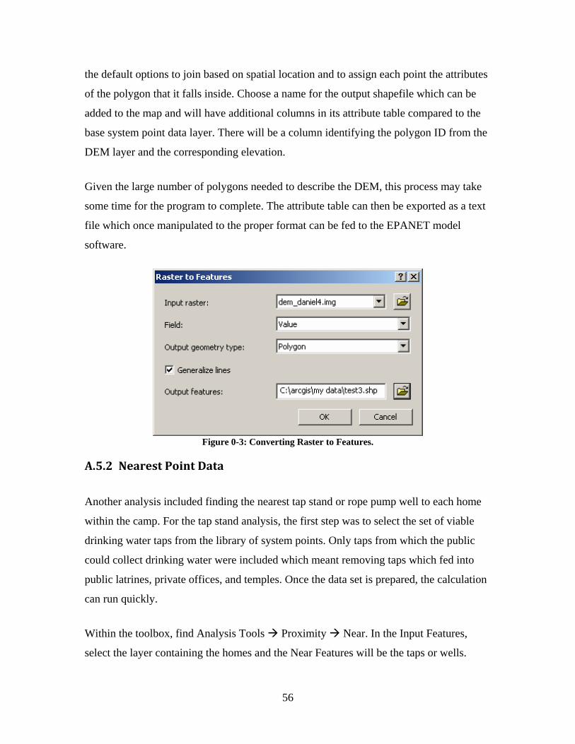
Given the large number of polygons needed to describe the DEM, this process may take
some time for the program to complete. The attribute table can then be exported as a text
file which once manipulated to the proper format can be fed to the EPANET model
software.
Figure 0-3: Converting Raster to Features.
A.5.2 Nearest Point Data
Another analysis included finding the nearest tap stand or rope pump well to each home
within the camp. For the tap stand analysis, the first step was to select the set of viable
drinking water taps from the library of system points. Only taps from which the public
could collect drinking water were included which meant removing taps which fed into
public latrines, private offices, and temples. Once the data set is prepared, the calculation
can run quickly.
Within the toolbox, find Analysis Tools Proximity Near. In the Input Features,
select the layer containing the homes and the Near Features will be the taps or wells.
57
Search radius can be omitted and make sure the desired units for distance are selected.
After some calculation time, the attribute table for the homes data set will have two more
important columns. “NEAR_FID” contains a number associated with the ID number of
tap or well which is closest to that particular home and “NEAR_DIST” is the distance to