Giulio Tiozzo Harvard University June 21, 2013

An entropic tour of the Mandelbrot set

Giulio TiozzoHarvard University

June 21, 2013

Summary

1. Topological entropy

2. External rays3. Main theorem, real version4. Complex version5. Sketch of proof (maybe)6. Remarks and conjectures

Summary

1. Topological entropy2. External rays

3. Main theorem, real version4. Complex version5. Sketch of proof (maybe)6. Remarks and conjectures

Summary

1. Topological entropy2. External rays3. Main theorem, real version

4. Complex version5. Sketch of proof (maybe)6. Remarks and conjectures

Summary

1. Topological entropy2. External rays3. Main theorem, real version4. Complex version

5. Sketch of proof (maybe)6. Remarks and conjectures

Summary

1. Topological entropy2. External rays3. Main theorem, real version4. Complex version5. Sketch of proof (maybe)

6. Remarks and conjectures

Summary

1. Topological entropy2. External rays3. Main theorem, real version4. Complex version5. Sketch of proof (maybe)6. Remarks and conjectures

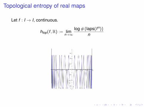
Topological entropy of real maps

Let f : I → I, continuous.

htop(f ,R) := limn→∞

log #{laps(f n)}n




log #{laps(f n)}n




log #{laps(f n)}n




log #{laps(f n)}n




log #{laps(f n)}n




log #{laps(f n)}n




log #{laps(f n)}n




log #{laps(f n)}n




log #{laps(f n)}n




log #{laps(f n)}n

Entropy measures the randomness of the dynamics.

Example: the airplane map

A 7→ A ∪ BB 7→ A

⇒(

1 11 0

)⇒ λ =

√5+12 = ehtop(fc ,R)


A 7→ A ∪ BB 7→ A

⇒(

1 11 0

)⇒ λ =



A 7→ A ∪ BB 7→ A

⇒(

1 11 0

)

⇒ λ =√

5+12 = ehtop(fc ,R)


A 7→ A ∪ BB 7→ A

⇒(

1 11 0

)⇒ λ =

√5+12

= ehtop(fc ,R)


A 7→ A ∪ BB 7→ A

⇒(

1 11 0

)⇒ λ =




log #{laps(f n)}n

Consider the real quadratic family

fc(z) := z2 + c c ∈ [−2,1/4]

How does entropy change with the parameter c?



log #{laps(f n)}n

Consider the real quadratic family

fc(z) := z2 + c c ∈ [−2,1/4]

How does entropy change with the parameter c?

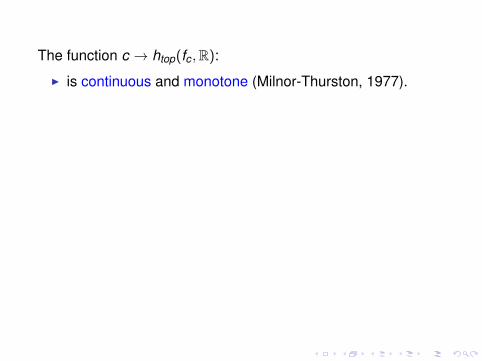
The function c → htop(fc ,R):

I is continuous and monotone (Milnor-Thurston, 1977).I 0 ≤ htop(fc ,R) ≤ log 2.


I is continuous

and monotone (Milnor-Thurston, 1977).I 0 ≤ htop(fc ,R) ≤ log 2.


I is continuous and monotone (Milnor-Thurston, 1977).

I 0 ≤ htop(fc ,R) ≤ log 2.





Remark. If we consider fc : C→ C entropy is constanthtop(fc , C) = log 2.

Mandelbrot set

The Mandelbrot setM is the connectedness locus of thequadratic family

M = {c ∈ C : f nc (0) 9∞}

External rays

Since C \M is simply-connected, it can be uniformized by theexterior of the unit disk

ΦM : C \ D→ C \M

External rays

Since C \M is simply-connected, it can be uniformized by theexterior of the unit disk

ΦM : C \ D→ C \M

External raysSince C \M is simply-connected, it can be uniformized by theexterior of the unit disk

ΦM : C \ D→ C \MThe images of radial arcs in the disk are called external rays.Every angle θ ∈ S1 determines an external ray

R(θ) := ΦM({ρe2πiθ : ρ > 1})

An external ray R(θ) is said to land at x if

limρ→1

ΦM(ρe2πiθ) = x



R(θ) := ΦM({ρe2πiθ : ρ > 1})An external ray R(θ) is said to land at x if

limρ→1

ΦM(ρe2πiθ) = x



R(θ) := ΦM({ρe2πiθ : ρ > 1})An external ray R(θ) is said to land at x if

limρ→1

ΦM(ρe2πiθ) = x

Rays landing on the real slice of the Mandelbrot set

Harmonic measureGiven a subset A of ∂M, the harmonic measure νM is theprobability that a random ray lands on A:

νM(A) := Leb({θ ∈ S1 : R(θ) lands on A})

For instance, take A =M∩R the real section of the Mandelbrotset. How common is it for a ray to land on the real axis?



For instance, take A =M∩R the real section of the Mandelbrotset.

How common is it for a ray to land on the real axis?



For instance, take A =M∩R the real section of the Mandelbrotset. How common is it for a ray to land on the real axis?

Real section of the Mandelbrot setTheorem (Zakeri, 2000)The harmonic measure of the real axis is 0.

However,the Hausdorff dimension of the set of rays landing on the realaxis is 1.

Real section of the Mandelbrot setTheorem (Zakeri, 2000)The harmonic measure of the real axis is 0. However,

the Hausdorff dimension of the set of rays landing on the realaxis is 1.

Real section of the Mandelbrot setTheorem (Zakeri, 2000)The harmonic measure of the real axis is 0. However,the Hausdorff dimension of the set of rays landing on the realaxis is 1.

Real section of the Mandelbrot setTheorem (Zakeri, 2000)The harmonic measure of the real axis is 0. However,the Hausdorff dimension of the set of rays landing on the realaxis is 1.

SectioningMGiven c ∈ [−2,1/4], we can consider the set of external rayswhich land on the real axis to the right of c:

Pc := {θ ∈ S1 : R(θ) lands on ∂M∩ [c,1/4]}









Pc := {θ ∈ S1 : R(θ) lands on ∂M∩ [c,1/4]}The function

c 7→ H.dim Pc

decreases with c, taking values between 0 and 1.


c 7→ H.dim Pc



c 7→ H.dim Pc



c 7→ H.dim Pc


Main theoremTheoremLet c ∈ [−2,1/4]. Then

htop(fc ,R)

log 2= H.dim Pc


htop(fc ,R)

log 2= H.dim Pc

Main theorem

TheoremLet c ∈ [−2,1/4]. Then

htop(fc ,R)

log 2= H.dim Pc

I It relates dynamical properties of a particular map to thegeometry of parameter space near the chosen parameter.

I Entropy formula: relates dimension, entropy and Lyapunovexponent (Manning, Bowen, Ledrappier, Young, ...).

I The proof is purely combinatorial.I It does not depend on MLC.I It can be generalized to (some) non-real veins.

Main theorem


htop(fc ,R)

log 2= H.dim Pc




Main theorem


htop(fc ,R)

log 2= H.dim Pc




Main theorem


htop(fc ,R)

log 2= H.dim Pc



I The proof is purely combinatorial.

I It does not depend on MLC.I It can be generalized to (some) non-real veins.

Main theorem


htop(fc ,R)

log 2= H.dim Pc



I The proof is purely combinatorial.I It does not depend on MLC.

I It can be generalized to (some) non-real veins.

Main theorem


htop(fc ,R)

log 2= H.dim Pc




In the dynamical planeDouady’s principle : “sow in dynamical plane and reap inparameter space”.

Each fc has a Julia set Jc .

In the dynamical planeDouady’s principle : “sow in dynamical plane and reap inparameter space”.Each fc has a Julia set Jc .

In the dynamical plane

Douady’s principle : “sow in dynamical plane and reap inparameter space”Each fc has a Julia set Jc .Let

Sc := {θ ∈ S1 : R(θ) lands on Jc ∩ R}

the set of rays landing on the real section (spine) of the Juliaset.


htop(fc ,R)

log 2= H.dim Sc = H.dim Pc


htop(fc ,R)

log 2= H.dim Sc = H.dim Pc

It also equals:I The entropy of the induced action on the Hubbard tree Tc

(minimal forward-invariant set containing the critical orbit),divided by log 2.

I The dimension of the set of biaccessible angles (Zakeri,Smirnov, Zdunik, Bruin-Schleicher ...)

CorollaryThe set of biaccessible angles for the Feigenbaum parameter(limit of period doubling cascades) cFeig has Hausdorffdimension 0.









The complex case: Hubbard treesThe Hubbard tree Tc of a quadratic polynomial is a forwardinvariant subset of the filled Julia set which contains the criticalorbit.

The complex case: Hubbard treesThe Hubbard tree Tc of a quadratic polynomial is a forwardinvariant subset of the filled Julia set which contains the criticalorbit.

Complex Hubbard treesThe Hubbard tree Tc of a quadratic polynomial is a forwardinvariant subset of the filled Julia set which contains the criticalorbit.

Complex Hubbard treesThe Hubbard tree Tc of a quadratic polynomial is a forwardinvariant subset of the filled Julia set which contains the criticalorbit. The map fc acts on it.

Topologically finite parameters

DefinitionA parameter c is topologically finite if its Hubbard tree ishomeomorphic to a finite tree.

Postcritically finite⇒ Topologically finite (but many more!)

PropositionIf c is biaccessible in parameter space (there are two distinctrays landing on c), then fc is topologically finite (i.e. on all veinsofM).


DefinitionA parameter c is topologically finite if its Hubbard tree ishomeomorphic to a finite tree.Postcritically finite⇒ Topologically finite

(but many more!)



DefinitionA parameter c is topologically finite if its Hubbard tree ishomeomorphic to a finite tree.Postcritically finite⇒ Topologically finite (but many more!)




PropositionIf c is biaccessible in parameter space (there are two distinctrays landing on c), then fc is topologically finite

(i.e. on all veinsofM).




Entropy of topologically finite parameters

Let c be topologically finite, with Hubbard tree Tc .

Let

Hc := {θ ∈ S1 : Rc(θ) lands on Tc}

TheoremLet fc be topologically finite. Then

h(fc ,Tc)

log 2= H.dim Hc


Let c be topologically finite, with Hubbard tree Tc . Let



h(fc ,Tc)

log 2= H.dim Hc


Let c be topologically finite, with Hubbard tree Tc . Let



h(fc ,Tc)

log 2= H.dim Hc

Entropy of Hubbard trees as a function of externalangle (W. Thurston)

Can you see the Mandelbrot set in this picture?

Entropy of Hubbard trees as a function of externalangle (W. Thurston)

Can you see the Mandelbrot set in this picture?

The complex caseA vein is an embedded arc in the Mandelbrot set.

The complex case

A vein is an embedded arc in the Mandelbrot set.

Given a parameter c along a vein, we can look at the set Pc ofparameter rays which land on the vein “below” c.

VeinsExistence of veins converging to dyadic angles[Branner-Douady, Kahn, Riedl].

For each p/q ∈ Q ∩ (0,1), there exists a unique parameter cp/qfor which:

I the rotation number around the α fixed point is p/q;I the critical point maps to the β fixed point after exactly q

iterates: f q(0) = β.

DefinitionThe principal vein vp/q in the p/q limb is the vein joining cp/q tothe center of the main cardioid.

I v1/2 = real axis;I v1/3 = Branner-Douady vein

The Hubbard tree for all parameters along vp/q is a q-prongedstar.

Pc := {θ ∈ S1 : RM(θ) lands on [0, c]}

VeinsExistence of veins converging to dyadic angles[Branner-Douady, Kahn, Riedl].For each p/q ∈ Q ∩ (0,1), there exists a unique parameter cp/qfor which:








I the rotation number around the α fixed point is p/q;

I the critical point maps to the β fixed point after exactly qiterates: f q(0) = β.























I v1/2 = real axis;

I v1/3 = Branner-Douady vein
























Complex versionTheoremLet vp/q be the principal vein in the p/q-limb of the Mandelbrotset, and let c ∈ vp/q. Then

htop(fc ,Tc)

log 2= H.dim Hc = H.dim Pc

Sketch of proof1. The rays landing on parameter space land also on the real

section of the Julia set:

Pc ⊆ Sc

2. In order to prove the reverse inequality, one would like toembed the rays landing on the Hubbard tree in parameterspace. This cannot be done in the renormalized copies.

3. However:

PropositionIf c is a non-renormalizable, real parameter, and c′ > c anotherreal parameter, there exists a non-constant, piecewise linearmap F : R/Z→ R/Z such that

F (Hc′) ⊆ Pc



Pc ⊆ Sc


3. However:


F (Hc′) ⊆ Pc



Pc ⊆ Sc


3. However:


F (Hc′) ⊆ Pc

Sketch of proof (continues)


F (Hc′) ⊆ Pc

4. By continuity,H.dim Hc = H.dim Pc

for non-renormalizable parameters.5. By renormalization, the same holds for all parameters

which are not infinitely renormalizable.6. By density of such parameters (in the space of angles), the

result holds.



F (Hc′) ⊆ Pc


for non-renormalizable parameters.

5. By renormalization, the same holds for all parameterswhich are not infinitely renormalizable.

6. By density of such parameters (in the space of angles), theresult holds.



F (Hc′) ⊆ Pc



which are not infinitely renormalizable.

6. By density of such parameters (in the space of angles), theresult holds.



F (Hc′) ⊆ Pc



which are not infinitely renormalizable.6. By density of such parameters (in the space of angles), the

result holds.

Pseudocenters

DefinitionThe (dyadic) pseudocenter of a real interval [a,b] with|a− b| < 1 is the unique dyadic rational number with shortestbinary expansion.

E.g., the pseudocenter of the interval [1315 ,

1415 ] is 7

8 = 0.111,since 13

15 = 0.1101 and 1415 = 0.1110.

Pseudocenters

DefinitionThe (dyadic) pseudocenter of a real interval [a,b] with|a− b| < 1 is the unique dyadic rational number with shortestbinary expansion.

E.g., the pseudocenter of the interval [1315 ,

1415 ] is 7

8 = 0.111,since 13

15 = 0.1101 and 1415 = 0.1110.

Bonus level: a bisection algorithm

TheoremLet c1 < c2 be two real parameters on the boundary ofM, withexternal angles 0 ≤ θ2 < θ1 ≤ 1

2 .

Let θ∗ be the dyadicpseudocenter of the interval (θ2, θ1), and let

θ∗ = 0.s1s2 . . . sn−1sn

be its binary expansion, with sn = 1. Then the hyperbolicwindow of least period in the interval (θ2, θ1) is the interval ofexternal angles (α2, α1) with

α2 := 0.s1s2 . . . sn−1

α1 := 0.s1s2 . . . sn−1s1s2 . . . sn−1

(where si := 1− si ). All hyperbolic windows are obtained byiteration of this algorithm, starting with θ2 = 0, θ1 = 1/2.



2 . Let θ∗ be the dyadicpseudocenter of the interval (θ2, θ1), and let

θ∗ = 0.s1s2 . . . sn−1sn

be its binary expansion, with sn = 1.

Then the hyperbolicwindow of least period in the interval (θ2, θ1) is the interval ofexternal angles (α2, α1) with

α2 := 0.s1s2 . . . sn−1

α1 := 0.s1s2 . . . sn−1s1s2 . . . sn−1





θ∗ = 0.s1s2 . . . sn−1sn


α2 := 0.s1s2 . . . sn−1

α1 := 0.s1s2 . . . sn−1s1s2 . . . sn−1





θ∗ = 0.s1s2 . . . sn−1sn


α2 := 0.s1s2 . . . sn−1

α1 := 0.s1s2 . . . sn−1s1s2 . . . sn−1





θ∗ = 0.s1s2 . . . sn−1sn


α2 := 0.s1s2 . . . sn−1

α1 := 0.s1s2 . . . sn−1s1s2 . . . sn−1

(where si := 1− si ).

All hyperbolic windows are obtained byiteration of this algorithm, starting with θ2 = 0, θ1 = 1/2.




θ∗ = 0.s1s2 . . . sn−1sn


α2 := 0.s1s2 . . . sn−1

α1 := 0.s1s2 . . . sn−1s1s2 . . . sn−1



Pseudocenters and maxima of entropy

DefinitionThe pseudocenter of a real interval [a,b] with |a− b| < 1 is theunique dyadic rational number with shortest binary expansion.

ConjectureLet θ1 < θ2 be two external angles whose rays RM(θ1), RM(θ2)land on the same parameter. Then the maximum of entropy onthe interval [θ1, θ2] is attained at its pseudocenter θ∗:

maxθ∈[θ1,θ2]

h(θ) = h(θ∗)



ConjectureLet θ1 < θ2 be two external angles whose rays RM(θ1), RM(θ2)land on the same parameter.

Then the maximum of entropy onthe interval [θ1, θ2] is attained at its pseudocenter θ∗:

maxθ∈[θ1,θ2]

h(θ) = h(θ∗)



ConjectureLet θ1 < θ2 be two external angles whose rays RM(θ1), RM(θ2)land on the same parameter. Then the maximum of entropy onthe interval [θ1, θ2] is attained at its pseudocenter θ∗:

maxθ∈[θ1,θ2]

h(θ) = h(θ∗)

Thurston’s entropy plot

Thurston’s quadratic minor lamination

A transverse measure on QML

Let `1 < `2 two leaves, and τ a transverse arc connecting them.

Then we defineµ(τ) := h(Tc2)− h(Tc1)

“Combinatorial bifurcation measure”?


Let `1 < `2 two leaves, and τ a transverse arc connecting them.Then we define

µ(τ) := h(Tc2)− h(Tc1)



Let `1 < `2 two leaves, and τ a transverse arc connecting them.Then we define

µ(τ) := h(Tc2)− h(Tc1)


The end

Thank you!

Coda: from Farey to the tent map, via ?

Minkowski’s question-mark function conjugates the Farey mapwith the tent map

0.2 0.4 0.6 0.8 1.0

0.2

0.4

0.6

0.8

1.0

0.2 0.4 0.6 0.8 1.0

0.2

0.4

0.6

0.8

1.0

0.2 0.4 0.6 0.8 1.0

0.2

0.4

0.6

0.8

1.0

Continued fractions ⇔ Binary expansions

The dictionary

Continued fractions ⇔ Binary expansions

E ←?→ R

α− continued fractions unimodal maps

numbers of generalized external raysbounded type on Julia sets

cutting sequences for univoque numbersgeodesics on torus(Cassaigne, 1999)

A unified approach

The dictionary yields a unified proof of the following results:

1. The real part of the boundary of the Mandelbrot set hasHausdorff dimension 1

H.dim(∂M∩ R) = 1

(Zakeri, 2000)2. The set of matching intervals for α-continued fractions has

zero measure and full Hausdorff dimension(Nakada-Natsui conjecture, Carminati-T. 2010)

3. The set of univoque numbers has zero measure and fullHausdorff dimension (Erdos-Horvath-Joo, Daroczy-Katai,Komornik-Loreti)

Entropy of α-continued fractions vs real hyperboliccomponents ofM

Date post:	06-Feb-2022
Category:	Documents
Upload:	others
View:	1 times
Download:	0 times

Giulio Tiozzo Harvard University June 21, 2013

Documents