Giving and Receiving Foreign Aid: Does Conflict Count? Eliana Balla (Federal Reserve Bank of Richmond, Banking Supervision and Regulation) • Gina Yannitell Reinhardt (Texas A&M University, Bush School of Government and Public Service) Keywords: foreign aid, political economy, economic development, conflict. JEL Classification: F3, O1. Abstract Do bilateral donors, whether for strategic or altruistic reasons, single out countries in or near a conflict as foreign aid recipients? We revisit the aid allocation debate, studying twenty bilateral donors over four decades. We find that allocation is based on the political and economic cooperation it could encourage, as well as on the economic development it could create. All donors condition aid on the presence of conflict, although in differing ways. The United States allocates large amounts of development aid to countries bordering a conflict, both pre- and post-Cold War, while donors traditionally seen as altruistic display strategic tendencies. • An earlier version of this paper was completed while both authors were at Washington University in St. Louis. We are grateful to Steve Fazzari and Gary Miller for reading, encouraging, and commenting on multiple drafts of this work. Lee Benham, Randy Calvert, Sebastian Galiani, Nate Jensen, Andrew Martin, Douglass North, Morgan Rose, and two anonymous referees provided additional valuable suggestions. We also thank Will Reinhardt, Andy Sobel, and the Center for New Institutional Social Sciences at Washington University for providing technical and financial support. Talgat Irisbekov and Esther Larson provided valuable research assistance. The views expressed in this article do not represent those of the Federal Reserve Bank of Richmond or the Federal Reserve System.
Transcript
Giving and Receiving Foreign Aid: Does Conflict Count?
Eliana Balla (Federal Reserve Bank of Richmond, Banking Supervision and Regulation)•
Gina Yannitell Reinhardt (Texas A&M University, Bush School of Government and
Public Service)
Keywords: foreign aid, political economy, economic development, conflict.
JEL Classification: F3, O1.
Abstract
Do bilateral donors, whether for strategic or altruistic reasons, single out countries in or
near a conflict as foreign aid recipients? We revisit the aid allocation debate, studying
twenty bilateral donors over four decades. We find that allocation is based on the
political and economic cooperation it could encourage, as well as on the economic
development it could create. All donors condition aid on the presence of conflict,
although in differing ways. The United States allocates large amounts of development
aid to countries bordering a conflict, both pre- and post-Cold War, while donors
traditionally seen as altruistic display strategic tendencies.
• An earlier version of this paper was completed while both authors were at Washington University in St. Louis. We are grateful to Steve Fazzari and Gary Miller for reading, encouraging, and commenting on multiple drafts of this work. Lee Benham, Randy Calvert, Sebastian Galiani, Nate Jensen, Andrew Martin, Douglass North, Morgan Rose, and two anonymous referees provided additional valuable suggestions. We also thank Will Reinhardt, Andy Sobel, and the Center for New Institutional Social Sciences at Washington University for providing technical and financial support. Talgat Irisbekov and Esther Larson provided valuable research assistance. The views expressed in this article do not represent those of the Federal Reserve Bank of Richmond or the Federal Reserve System.
2
To what extent do a donor’s strategic interests, those interests pertaining to its
short term and long term political and economic goals, condition bilateral aid allocation?
In extensive previous analysis of foreign aid allocation (see Akhand and Gupta 2002 for
review), scholars often characterize strategic donors as concerned with areas
experiencing or threatened by conflict, and attempt to capture their interests with
measures such as recipients’ proximity to Communist countries (McKinlay and Little
1977) and recipients’ human rights abuses (Poe 1992; Lai 2003). The debate remains,
however, as to whether aid flows toward contentious regions in the hopes of stabilizing
them, flows away from contentious regions until the strife dies down, or has any
relationship with conflict at all. Past works suggest that various types of conflict, be they
internal or between superpowers, have an impact on aid allocation, but none target and
measure conflict systematically.
We add a new dimension to donors’ strategic motivations: the recipient’s
geographic proximity to conflict. Geographic proximity to conflict is an improvement
over previous measures of strategic interest in that it allows comparison across several
donors in one framework, rather than relying on region invariant effects, or a division of
time based on the Cold War.1 Examining 20 bilateral donors and 122 recipients, we
confirm previous findings that there are economic, political, and altruistic elements to
allocation for most donors, although to varying extents in each. We also assess conflict
in the context of a two-stage aid allocation decision, and find that a recipient’s
1 Alesina and Dollar (2000) are the only scholars to date that undertake as inclusive an analysis of bilateral donors, although they do not analyze the presence and/or intensity of conflict, and they cover a subset (1970-1994) of the years and donors in this study.
3
geographic proximity to conflict holds explanatory power for every donor in our study.
The US, Norway, Italy, Germany, Finland, and the USSR condition aid positively on
geographic proximity to conflict, while Canada, France, Switzerland, and Spain indicate
a preference for allocation in more stable environments. Many donors traditionally
viewed as altruistic display strategic features, when conflict is taken into account.
A deeper understanding of allocation patterns sheds light on aid effectiveness.2
Because we find that bilateral aid is given largely as a result of donors’ political and
economic interests, we can surmise why aid is not as effective at spurring development as
proponents originally hoped it would be. Strategic donors do not necessarily allocate aid
based on the development it could create, but rather on the cooperation it could
encourage. Conflict, always known to be potentially devastating to a nation’s economic
and political system, may threaten it in ways previously not pondered – specifically, the
reduction of aid. It is thus important to determine which donors are strategic in their
allocation, and what elements of strategic allocation can be observed systematically.
I. Conflict and Allocation
Typically, studies of the determinants of bilateral foreign aid allocation focus on
the motives of bilateral donors, and target two main dimensions: altruistic and strategic.
Altruistic motivations are based on humanitarian interests in a recipient’s development
levels. Altruistic donors target aid toward countries that can use the money most
effectively to bolster savings levels and increase the general welfare.
2 See Burnside and Dollar (2000) for analysis of when aid is effective for development.
4
Strategic motivations are those associated with the donor’s short term and long
term political and economic interests. Friedman (1958) noted early in the history of aid
that it might be used as a tool by donors to win allies. Although he believed such an
intention to be misguided, further scholarship has characterized various donors,
particularly the US, as being strategic in allocation motives (McKinlay and Little 1977).
If a donor seeks future political or economic cooperation from a given developing
country, it may allocate aid to that recipient to enable it to respond to donor requests, to
insure the recipient will remain a faithful ally (Mosley 1986: 32), or to give it a greater
disposition to cooperate with the donor in international affairs.
In such a case, strategic importance would trump “need” as a determinant of
allocation levels (ibid.). The strategic donor thus hopes to fund only those recipients that
will, or have the potential to, cooperate. Before aid is allocated, it is impossible to be
certain if aid will encourage a given recipient to cooperate. The donor therefore hopes to
find the ideal recipient at the onset, before making its final allocation decision, and seeks
clues that will indicate a potential recipient’s willingness to cooperate in the future.
The principal-agent paradigm is a useful means to characterize this donor-
recipient relationship. The donor is the principal, seeking its ideal recipient amongst a
field of possibilities. The recipient is the agent, which cannot be monitored constantly to
insure that the aid will have the effect the donor desires. Thus, the donor attempts to
avoid adversely selecting aid recipients for which aid will not encourage cooperation or
development. It tries to determine at the onset which recipients are appropriate by
looking for signals that can be associated with future cooperation. After deciding which
5
recipients will receive its aid (the gate-keeping decision), the donor must then determine
how much aid each recipient will get (the level-setting decision).3 We thus follow the
lead of Cingranelli and Pasquarello (1985), in their characterization of the allocation
decision as a two-stage process. Both the gate-keeping decision and level-setting
decisions are influenced by the donor’s assessment of a recipient’s cooperation potential.
This assessment is likely based both on previous cooperation between the donor and
recipient, as well as recipient attributes that make its cooperation with the donor
desirable.
Often scholars try to capture the altruistic dimension of aid by gathering data on
recipient development levels such as Human Development Indicators (HDI), GDP,
literacy rates, and mortality rates (see Polachek, Robst, and Chang 1999). Strategic
motives have been measured by analyzing United Nations General Assembly (UNGA)
voting relationships (Alesina and Dollar 2000), trade and treaty memberships (Meernik,
Krueger, and Poe 1998), colonial history, human rights records (Poe and Tate 1994), and
levels of democracy. Most of these studies focus on one donor at a time, to insure that
case-specific interests are included in the study. Empirical studies indicate that donors
have varying ways of avoiding the adverse selection problem. France is seen as giving
aid largely based on colonial ties. Japan gives aid to trading partners. The US gives a
large portion of aid to the Middle East, and during the Cold War gave substantial aid to
nations bordering Communist countries (McKinlay and Little 1977).
3 Martens et al (2002) has characterized the chain of foreign aid allocation as a series of principal-agent problems. See Laffont and Martimort (2001) for presentation of the basic principal-agent model and the adverse selection problem.
6
Yet even within these depictions of donor preferences, examinations into
allocation patterns exhibit variations in allocation that cannot be explained by the usual
suspects. We thus need to cast a different paradigm, one which enables all donors to be
examined by the same criteria, one which gives us a continuous look at strategic interests
that is not divided by the presence or absence of the Cold War. We create a new variable,
geographic proximity to conflict, to enable us to understand donor strategic interests in
the context of both the Cold War and the years since it ended. A nation’s relationship to
conflict can be described on two dimensions: proximity and intensity. In a given year, a
recipient can have one of four levels of proximity: harboring a conflict, bordering a
conflict, being in the region of a conflict, or being near no conflict at all. The intensity of
any conflict has three possible ratings: minor (more than 25 battle-related deaths per
year), intermediate (more than 25 battle-related deaths per year and a total conflict history
of more than 1000 battle-related deaths), or high (more than 1000 battle-related deaths –
war).4
We posit that conflict is a mitigating contextual variable in the typical principal-
agent story, which can affect allocation patterns through three basic mechanisms.
Altruistic donors might increase aid to nations that are threatened with conflict, in order
to secure basic human rights and services (see Polachek, Robst, and Chang 1999). Some
strategic donors may wish to stabilize recipients from whom they need future cooperation
(see Stein, Ishimatsu, and Stoll 1985), or to gain access to a nation geographically near a
4 These variables were culled from the Armed Conflict Dataset from the International Peace Research Institute, Oslo (PRIO), authors Havard Strand, Lars Wilhelmsen, & Nils Petter Gleditsch (2002). Please see further details accompanying Figure 1.
7
particular conflict. Other strategic donors, concerned that their aid yield the highest
payoff possible, may target stable environments, eschewing those with conflicts.
Previous scholarship discusses the link between conflict and allocation with
specific examples. Aid to Southeast Europe spiked in 1999 after the Kosovo Crisis
threatened to destabilize the region (Mitra et al 2001), illustrating the interdependence
between one recipient’s aid levels and the conflict its neighbors endure. After the war in
Bosnia and Herzegovina that ended in 1994, aid levels approached 75% of GDP
(Demekas et al 2002). Also in 1994, when genocide in Rwanda gained international
notoriety, aid to Rwanda increased by $280 million,5 over 29% of GDP.
An examination of bilateral aid flows from 1960-1997 shows further variations in
both conflict and aid. Take France, often cited as giving aid heavily to past colonies.
Sixteen recipients in Sub-Saharan Africa were colonies of France, yet receive disparate
amounts of gross aid from France during the time examined. Of these sixteen recipients,
nations bordering conflicts received, on average, $19 million more per year than those
not bordering or containing a conflict. Figure 1 illustrates that over time, recipients
bordering conflicts received more than those containing conflicts, as well. Within nations
bordering conflicts, those bordering high intensity conflicts receive $51 million less in
French aid per year than those bordering intermediate conflicts, and $32 million less per
year than those bordering minor conflicts.
(Insert Figure 1 about here.) 5 The average differences presented in this section are the result of a Scheffé multiple-comparison test run on OECD data (see appendix for source information and definitions), which measures the difference in means between two categories and tests whether that difference is significantly different from zero (see Hamilton 2004, 150-151). All tests are performed on data given per country-year in 1995 US dollars and are significant at the p<.05 level.
8
Or, consider the argument that Japan conditions aid in part based on trading
relationships. Focusing on the nations that maintain trading volumes above the median
with Japan, we find that those that harbor conflicts receive an average of $120 million
more per year, and those that border conflicts receive an average of $46 million more per
year, than those that are merely in the region of a conflict, regardless of the intensity of
that conflict. Figure 2 visually depicts these values over time, showing that although
there is a steady trend upward in Japanese aid overall, money is more likely to go to
trading partners containing conflicts than those that do not. Considering only nations
with proximity to high intensity conflicts, those in the region of high intensity conflicts
receive, on average, $50 million less per year than those with internal high intensity
conflicts, and $47 million less per year than those bordering high intensity conflicts.
(Insert Figure 2 about here.)
The Middle East is often considered to be a region of strategic importance to the
US, largely due to its geopolitical significance. Within Middle Eastern recipients of US
aid, nations containing conflicts receive an average of $470 million more than those in
the region of a conflict, per year. Holding intensity constant at the intermediate level,
those harboring intermediate conflicts receive an average of $570 million per year more
than those bordering similar conflicts, and $680 million more per year than those in the
region of similar conflicts. Considering nations with internal conflicts, those harboring
high intensity conflicts receive an average of $760 million less per year than those with
intermediate conflicts (see Figure 3).
(Insert Figure 3 about here.)
9
These variations in aid flows over time indicate that a recipient’s proximity to
conflict, as well as a given conflict’s level of intensity, may have profound effects on
allocation patterns despite controlling for variables such as region, development levels,
population size, and strategic considerations of trade and colonial history. We thus set
out to investigate conflict as a previously omitted component of allocation in multivariate
analysis. While acknowledging that not all donors are strategic in their allocation, we
move on to explore the donor that is strategic, basing allocation in part on short term and
long term economic and political interests. We expect each donor to have a different
preference ordering over altruistic and strategic interests, but we set out to test them all
according to the same model, in order to compare interest profiles.
II. Data, Hypotheses, and Estimation
We conceptualize the allocation process in two stages: gate-keeping and level-
setting. We include conflict in or near the recipient at both the gate-keeping and level-
setting stages to examine the effects of this potential determinant of allocation. For every
donor data set, each observation represents a recipient in a given year, spanning 122
recipients from 1960-1997 (see Table A1 in the appendix for a list of recipients). We
examine all potential bilateral relationships between any countries that were aid
recipients during this period and each of the donors for which bilateral aid data was
available.6 Table A2 in the appendix presents variable definitions, sources, and
6 The donors for which we were able to retrieve data are: Australia, Austria, Belgium, Canada, Denmark, Finland, France, Germany (pre-unification, this data set accounts for West Germany), Ireland, Italy, Japan, Netherlands, New Zealand, Norway, Portugal, Spain, Switzerland, Sweden, UK, US, and USSR. Each donor recipient panel is unbalanced. Due to the nature of developing countries’ data, many observations of the control variables drop out of various regression specifications. There is a concern that data for certain countries may be missing systematically (e.g. from the least developed Sub-Saharan African countries),
10
descriptive statistics. Our dependent variable is gross per capita bilateral aid, in constant
1995 US dollars, flowing from a given donor to a given recipient in a given year.
Gate-Keeping Stage
In the gate-keeping stage, a donor decides whether to allocate aid to a potential
recipient. For this stage of our empirical specification, we turn the aid measure of the
dependent variable into a dummy that takes value 1 if the variable is observed and 0
otherwise. We also lag the dummy variable and use it as a regressor in this stage to
account for the bureaucratic inertia embedded in the aid allocation process and the lock-
in effect associated with aid projects that last multiple years.7
We posit that this stage will be determined in part by a donor’s altruistic interests,
and thus that the chance for observation is affected by a recipient’s degree of economic
development. We capture these altruistic interests with lagged controls of GDP per
capita and life expectancy, which we expect to be negatively correlated with aid.
Additionally, conflict-stricken areas may receive altruistically-motivated aid to help
strengthen economies and social structures.
The gate-keeping stage should also be determined by those strategic interests that
indicate cooperation between the donor and the recipient. We capture a history of
cooperation between the donor and recipient by including bilateral trade patterns, past
colonial ties, the nature of a country’s political regime through its Polity IV score, and
voting history in the UNGA. We expect that trading partners and previous colonies will
potentially biasing our results. Comparisons across donors should still be valid if the bias is similar across donor regressions. 7 Existing literature omits the lagged dependent variable in aid allocation estimations. The fit of the model improves when lagged aid is included in the selection rather than the regression stage.
11
be more likely to receive aid from economically oriented donors than other recipients.
We hypothesize that a country’s Polity IV score, which ranks the political regime of a
recipient from most autocratic to most democratic (-10, 10), as well as a strong voting
relationship over the previous five years with a particular donor, will have positive effects
on the likelihood of receiving aid from politically oriented donors.8
We also include measures of conflict in the gate-keeping stage, to examine the
effects of conflict proximity as it grows closer to each recipient, as well as the effects of
increases in conflict intensity, on whether or not a nation will receive aid from a given
donor. The effect of aid during a conflict can be ambiguous. On the one hand, conflict
increases the aid recipient’s needs; on the other it raises rents to be captured by winners.
For example, the Grossman (1992) model explores the effect of aid on conflict risk and
predicts that it will make conflict more likely. Aid is a financial prize of rebellion in this
model. Because it can be reasonable for donors to either grant or withhold aid based on
conflict, we do not hypothesize a particular direction of association between conflict and
aid at this stage, but we do expect that donors will condition aid on conflict in some way.
Lastly, we control for region9 and population10 in the gate-keeping stage.
8 The exception to this expectation is the USSR’s gate-keeping stage, with which the Polity IV score should have a negative relationship. 9 Regional dummies account for region invariant effects. Alternatively, we test our hypotheses for key donors in different regions. Including regional effects is more reliable as it affords estimation with pooled observations. It also allows us to broaden our attention beyond the Middle East effect that has been largely explored by previous scholarship. To relate to this previous work, we use the Middle East as baseline. 10 A small-country bias, first identified by Isenman (1976), would exist if smaller states received more aid per capita than larger states. One reason for this might be because each state might be useful in terms of future cooperation, and thus smaller states, when receiving an amount of aid that is not “derisory,” would be able to spread that amount over fewer people (632). Controlling for population size will account for this potential bias.
12
Level-Setting Stage
In the level-setting stage, we incorporate the most recent cooperation indicators
available to the donor. Altruistic indicators may play a role at the level-setting stage, so
GDP per capita, life expectancy, and population serve as potential indicators for the need-
based aid amount allotted to different recipients.11 To capture strategic considerations,
we include recent voting correlations and conflict variables. We expect the proximity
and intensity of a conflict to thus influence not only whether a nation will be a recipient,
but also how much aid it receives.12
Estimation
As a donor’s decision to allocate aid to a recipient is unlikely to be random, we
elect not to use ordinary least squares regression to fit an aid allocation model. Our data
set indicates that donors do not allocate funds to all recipients in all years, and that the
proportion of observations where no allocation occurs is significant. Least squares
regressions such as reported in Alesina and Dollar (2000) applied to the aid allocation
problem yield biased results if there is a non-zero correlation between the gate-keeping
stage and the level-setting stage. Instead, we fit the following Heckman selection model,
estimated with maximum likelihood, which potentially produces consistent,
asymptotically efficient estimates for all the parameters in the aid allocation model.13
11 Certain variables, such as past colonial history, are not applicable to all donors. With few exceptions, however, all donor regressions are based on the same criteria. 12 Geographic proximity to conflict is likely correlated with needs of the recipient when the recipient itself is the territory of a conflict. Refugees may also raise the need for aid in bordering countries. Much of this need, however, would be reflected in relief aid, which this study does not include. 13 Because the data is censored due to a binary decision that each donor makes whether to allocate aid to a recipient in a given year, we choose a Heckman selection model over a Tobit analysis. We believe the aid allocation decision to be two-stage (selection stage: fund or not fund, outcome stage: how much to fund),
13
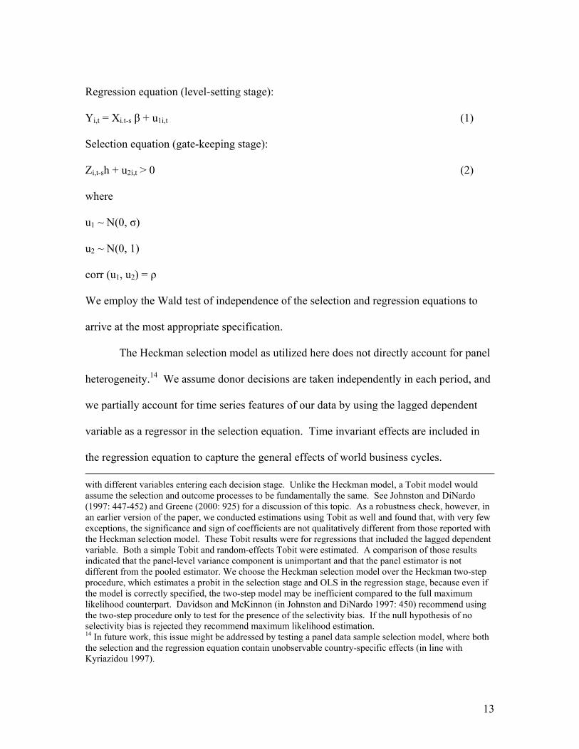
Regression equation (level-setting stage):
Yi,t = Xi.t-s β + u1i,t (1)
Selection equation (gate-keeping stage):
Zi,t-sh + u2i,t > 0 (2)
where
u1 ~ N(0, σ)
u2 ~ N(0, 1)
corr (u1, u2) = ρ
We employ the Wald test of independence of the selection and regression equations to
arrive at the most appropriate specification.
The Heckman selection model as utilized here does not directly account for panel
heterogeneity.14 We assume donor decisions are taken independently in each period, and
we partially account for time series features of our data by using the lagged dependent
variable as a regressor in the selection equation. Time invariant effects are included in
the regression equation to capture the general effects of world business cycles. with different variables entering each decision stage. Unlike the Heckman model, a Tobit model would assume the selection and outcome processes to be fundamentally the same. See Johnston and DiNardo (1997: 447-452) and Greene (2000: 925) for a discussion of this topic. As a robustness check, however, in an earlier version of the paper, we conducted estimations using Tobit as well and found that, with very few exceptions, the significance and sign of coefficients are not qualitatively different from those reported with the Heckman selection model. These Tobit results were for regressions that included the lagged dependent variable. Both a simple Tobit and random-effects Tobit were estimated. A comparison of those results indicated that the panel-level variance component is unimportant and that the panel estimator is not different from the pooled estimator. We choose the Heckman selection model over the Heckman two-step procedure, which estimates a probit in the selection stage and OLS in the regression stage, because even if the model is correctly specified, the two-step model may be inefficient compared to the full maximum likelihood counterpart. Davidson and McKinnon (in Johnston and DiNardo 1997: 450) recommend using the two-step procedure only to test for the presence of the selectivity bias. If the null hypothesis of no selectivity bias is rejected they recommend maximum likelihood estimation. 14 In future work, this issue might be addressed by testing a panel data sample selection model, where both the selection and the regression equation contain unobservable country-specific effects (in line with Kyriazidou 1997).
14
Additionally, year effects may reveal features of a donor’s domestic optimization
problem about how much aid it can afford, subject to domestic constraints.15 We attempt
to uncover the strategic interaction between donors and recipients in addition to the
determinants of trends of bilateral aid allocation.16 To that purpose, we estimate our
model with annual data, which allow for observing short-term behavior alterations on the
part of donors and recipients, rather than averages over a range of years, which are more
suited for studying behavioral trends. To control for the possibility of simultaneity and
allow for information lags, all independent variables are lagged once.
III. Empirical Results
We find that donors vary in their degree and type of strategic interests.
Geographic proximity to conflict, while consistently holding significance, points to
differential and intricate donor and recipient behavior (see Tables 1 and 2 below). Table
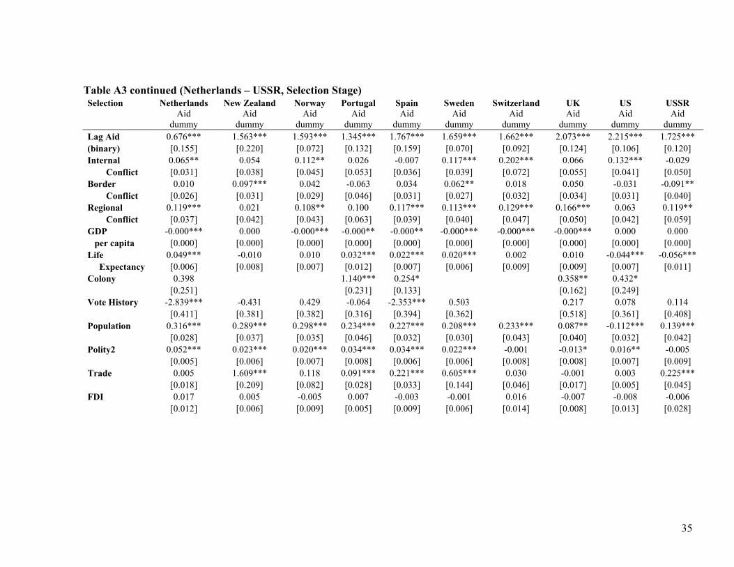
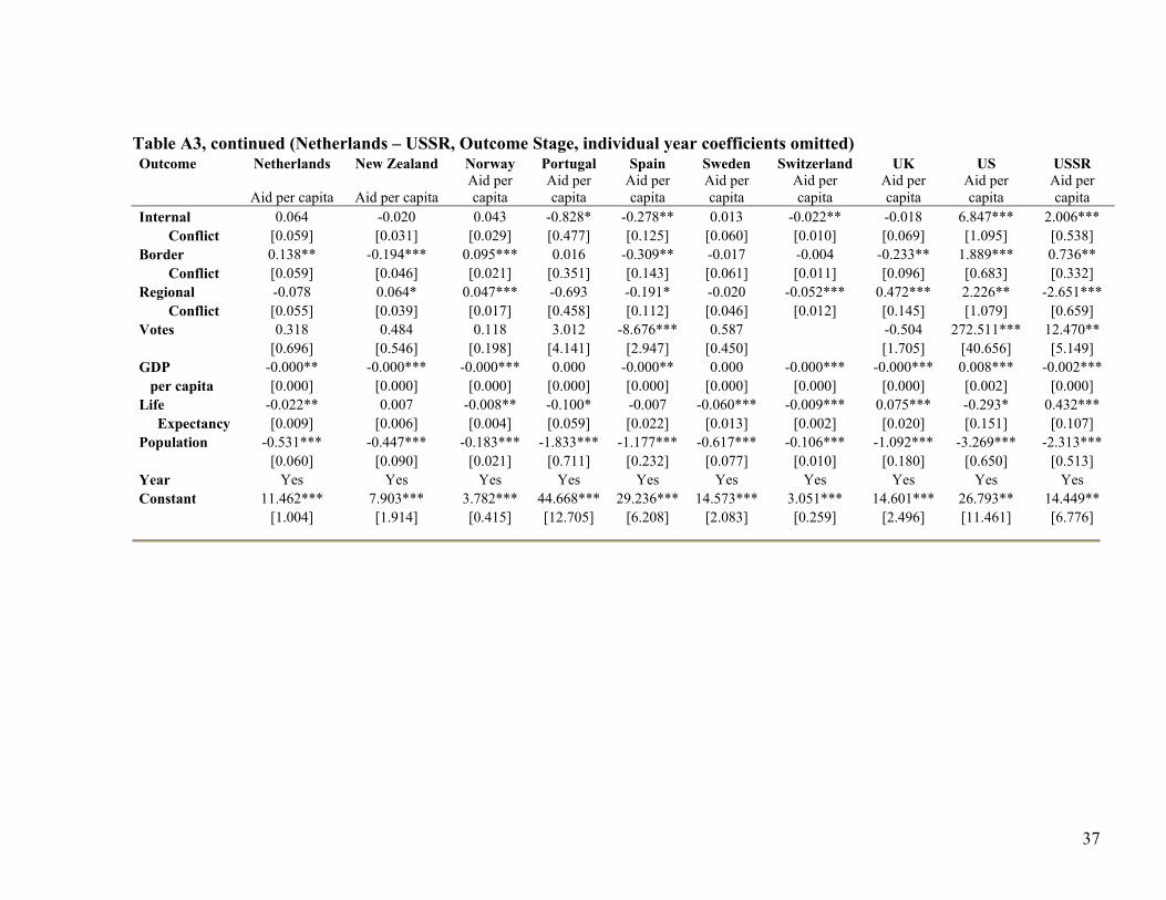
A3 in the appendix presents our raw findings from individual donor estimations. For
eighteen donors, a Wald test17 confirms the validity of the Heckman selection model.18
15 A direct address of the donor’s decision of how much total aid to allocate given a budget constraint or how to partition its aid resources between bilateral and multilateral aid is beyond the scope of this paper. 16 It is possible that aside from the strategic interaction between donors and recipients, donors themselves interact in the allocation process in ways unaccounted for thus far. One donor may decide to follow the lead of another, allocating resources in a bandwagon effect to pool resources or save information costs. The opposite relationship may exist; donors may reduce aid to recipients heavily supported by other countries out of altruistic concerns towards the lesser recipients. Controlling for these effects is difficult. If the total aid of all other donors is used as a control in, for example, the US regression, the two effects may counteract each other, casting doubt on the usefulness of this measure. Also, simultaneity between the total amount of aid available for distribution and that allocated to each country may pose a serious econometric problem, given that total aid depends on the assessment of need or donor interest in recipient countries. As a robustness check, in an earlier version, we included “amount of aid by all other donors” in unreported regressions of individual donors to find that this inclusion does not alter the explanatory power of other variables in either the selection or the regression stage. Further, including aid disbursement of a specific donor (e.g. including US distribution in the France regression) does not change the results on variables of interest. 17 The Wald test rejects the hypothesis that the correlation coefficient between the selection and regression stage equals zero, and is reported at the bottom of Table A3.
15
The estimations of Austria’s and Germany’s aid allocation do not pass this test, whereas
Australia’s results are unreliable as the estimation fails to converge under acceptable
terms. We therefore omit the Australian results, and caution the reader that the Austrian
and German results are to be interpreted with care. Table A3 provides guidance on the
qualitative findings of our study by indicating the significance and direction of the effect
of the independent variables on either the likelihood that a country becomes an aid
recipient, or that a country receives a certain amount of aid.
The magnitude of all the coefficients interpreted below is from Table 1. The
coefficients represent marginal effects of each independent variable on the aid dependent
variable. The marginal effects reported (see the legend to Table 1 for background on
computation) are conditional on the aid observation taking a positive value and for values
of the rest of the explanatory variables kept constant at their means. If a variable enters
both estimation stages, that variable’s combined effect is reported. Marginal effects are
also reported for the regressors whose explanatory power is only included in the selection
stage. In the interest of space, we focus on discussing those donor regressions that raise
more interesting orders of magnitude or that display effects previously unaccounted for in
the literature.
Conflict
Consider first geographic proximity to conflict. The main results are summarized
in Tables 1 and 2 below. We find that the presence of a conflict (whether internal or
18 We have concerns about any inferences based on the USSR regression because OECD data were incomplete for the aid and trade variables. Additionally, for some of the likely receivers of USSR aid (the former Eastern Bloc), we were only able to obtain post-1990 data for the control variables.
16
bordering)19 increases the propensity that fourteen of the donors will select a recipient
(Austria, Belgium, Finland, France, Germany, Ireland, Italy, Japan, Netherlands, New
Zealand, Norway, Sweden, Switzerland, and the US fall into this category; see Table
A3).20 A non-overlapping group of fourteen donors also allocate aid to countries in the
region of a conflict. For nine donors, an increasingly intense internal conflict reduces the
amount of aid to that country, suggesting that while many donors are more likely to give
aid to recipients bordering or experiencing conflicts, once those recipients have passed
the gate, they receive less aid than otherwise.
Spain joins Canada, New Zealand, and the UK in reducing aid to recipients
bordering intense conflicts. Denmark, Finland, Netherlands, and Norway, join the US,
Japan, Germany, and Ireland in increasing aid to countries bordering more intense
conflicts. These findings suggest the possibility that these donors attempt to stabilize a
neighbor of a conflict due to economic and/or political motivations.
The magnitude of the effect of the conflict variables is profound for a number of
donors. For instance, a change of one standard deviation in the variable measuring
internal conflict intensity, from a mean value of .44 to a value of 1.38, is associated with
a US$6.59 increase in US aid per capita (47% of mean), and a US$1.79 increase (11% of
mean) in Soviet aid per capita. At the opposite end, France withholds US$.76 (7.53% of
mean) for the same change in internal conflict intensity.
19 For consistency, we allowed for the regional presence of conflicts in the selection stage, while agreeing that the region-invariant effects already account for features of the region. 20 Being in the region of a conflict, for the most part, does not induce donors to pull away from aid giving, the exception being the US and the USSR, which allocate less aid to these peripheral countries.
17
(Insert Table 1 about here)
The variable measuring border conflict intensity displays similarly mixed results.
The US stands at the far end on funding recipients bordering a conflict, increasing its aid
by US$2.46 per capita per one standard deviation increase in bordering conflict intensity.
This corresponds to 17.4% of mean US aid per capita. The UK, instead, reduces its aid to
countries bordering a conflict by US$3.12 per capita, 76% of the UK mean aid.
Our findings show that some donors prefer stable environments for their aid
investment, while many others are willing to fund countries housing or in close proximity
to a conflict. The intensity of any given conflict magnifies the positive or negative effect
in the amounts exemplified above. The US and USSR on average exhibit higher orders
of magnitude in these effects, in part due to the higher aid amounts they allocate.21
(Insert Table 2 about here)
Recall the mechanisms we posit, above, by which conflict can influence aid
allocation. Those giving more aid based on conflict may be trying to gain access to those
conflicts or to influence the outcome. Those giving less aid based on conflict may be
concentrating their scarce resources on recipients that they deem more stable, and thus
more able to cooperate economically and politically in the future. This would explain
why the US and the USSR, the donors with the most aid to give, are able to allocate aid
21 To examine whether the salience of a vote could increase during times of conflict, we multiplied the voting scores of donor-recipient pairs by the dummies reflecting degrees of proximity to a conflict. These coefficients are generally harder to interpret and demonstrate that no significantly new information is gained through their inclusion. The interactions hold significance only sporadically and for few donors. They are thus excluded from the specification discussed here. The only result of potential interest is the case of internal conflict in the US regression, where we observe a significant statistical and economic effect on the interaction term. This effect does not disappear when dummies for Egypt and Israel are included in the estimation, Egypt and Israel being well known cases of high receipts of US aid and likely candidates of a conflict such as the above.
18
to conflict-stricken areas, and why the smaller donors reduce allocation to areas of
intense conflict.22
UNGA Voting
The importance of the conflict variables should be further assessed in comparison
with our control variables. We turn to the UNGA voting correlations as a summary
measure of donor-recipient alliances. The voting history coefficient is positive for 13 of
the 18 donors. Positive coefficients are statistically different from zero at a 10 percent
level or less for five donors (Austria, Finland, France, Germany, and Japan). The
Netherlands, Spain, and Ireland have negative and significant coefficients, possibly
suggesting that this friendship measure is inappropriate in cases where a single variable
(e.g. ex-colonial ties for Spain) determines the vast majority of a donor’s allocation
decision.
Recent UN votes also show significant effects on aid distribution. A particularly
notable finding is the effect of recent voting in the US regression, where moving from a
voting correlation of 0.15 to 0.35 (from about the 25th to the 75th percentile of all votes)
adds an astounding US$54.50 per capita to a recipient’s aid, a quadrupling of the mean.
For the same percentile move, going from a 0.32 to 0.48 correlation adds roughly
US$0.42 per capita to German aid, a 13 percent increase over the mean. It is striking that
22 The US and USSR were also the key players in the Cold War, suggesting that these findings reflect their desire to foster cooperative regimes. We have no indication that US allocation behavior regarding conflict is limited to the Cold War Era. We performed more in-depth examinations of key donors via sub-sample regressions to check for differential behavior of a single donor across regions and/or time. When sub-sample estimations were attempted, the Heckman procedure had difficulties converging in numerous occasions and/or the results were too close to boundary conditions to be trustworthy. One result that we can interpret is that US correlations with regard to voting patterns and geographic proximity to conflict hold temporally (in regressions by decade).
19
the Scandinavian countries, typically seen as more altruistic in motive, exhibit
correlations between aid and recent voting: Denmark and Finland, for example, seem to
“reward” most recent cooperation in the UNGA, while others do not seem to take the
most recent known votes as a representation of alliance. The coefficients of recent votes
for Belgium, Ireland and Spain suggest that votes are not viewed strategically by these
donors. As it may be the case with historical votes, such countries might look to other
indicators (e.g. trade relations, past colonial ties, and the nature of the recipient’s political
regime) as a sign of alliance.
Relationships among donors themselves may help explain the negative
coefficients as well. If two donors from different UN coalitions share aid recipients,
these recipient countries can use their vote as a signal of alliance with one donor only.
The pattern of the coefficients on voting correlations (both voting history and recent
votes) suggests that many, but not all, donors may view votes strategically. Overall, we
assess that bilateral aid is appreciably channeled into recipients who maintain friendly
relations with donors in the UN.
There is a concern with the endogeneity of UNGA votes and aid allocation.
Lundborg (1998), for example, finds that smaller countries receive proportionately more
aid, and suggests that aid from the US and USSR influenced and was influenced by votes
in the UNGA. Because the UNGA operates under the one-country-one-vote rule, an
efficient vote-buying strategy would target small countries. This potential simultaneity
problem has been raised and addressed by Alesina and Dollar (2000) who, after
instrumenting for UNGA votes, deduce that the more likely direction of causality goes
20
from votes to aid allocation rather than the other way around. We treat the voting
correlation with a donor of interest (as defined by the statistical significance of this
variable) as a possibly endogenous covariate, instrumenting for it with another donor’s
voting correlation. Our limited results are consistent with previous findings in the
literature.23
In order for funding to occur, donors prioritizing strategy over altruism must have
a higher belief, relative to that required by more altruistic donors, that a targeted recipient
is an ally. In reality, the prior belief of whether a donor is an ally or not is based on
evidence of previous economic and political cooperation. Therefore, if we observe that a
donor conditions aid on UN votes and/or conflict, we should also observe that the other
cooperation variables (economic partnerships, previous colonial ties, past aid
relationships) are important to allocation. Below, we discuss the evidence of these
observations.
Control Variables
There is a path dependence effect in allocation that becomes apparent in our
study. Having received aid the year before consistently increases the probability of
selection as an aid recipient in all donors (except Austria and Germany—possibly the
reason why the fit of these particular donors is inadequate). The effect of lagged aid
varies in magnitude. It is smallest for the UK, Switzerland, and Japan at 10-15 percent
23 We choose Japan as the instrumenting donor because it exhibits consistently high voting correlations with the other donors while it targets a relatively distinct group of aid recipients. In the Japan regression, we use Norway as the instrumenting donor. Because the Heckman specification cannot accommodate instrumental variables, we focus on the gate-keeping stage and estimate a probit model that allows for endogenous covariates. A Wald test of exogeneity suggests that we cannot reject the hypothesis that voting correlations are exogenous. Note that we cannot generalize this result across all donors as the underlying assumptions of this technique are not always met.
21
above their respective aid means, and highest for Spain and New Zealand at 366% and
437% over their respective means. Other donors fall in between these two extremes. For
example, being a recipient of Swedish, US, French, and USSR aid the year before
increases current aid levels by US$1.04 (85% over the mean), US$4.50 (32% over the
mean), US$6.92 (74% over the mean), and US$5.42 (32% over the mean) per capita in
their respective regressions.
We now turn to observations about the more traditional political and economic
determinants of aid allocation. The interactions of good institutions, aid, and economic
growth have received much attention from researchers and aid policy-makers since the
late nineties (beginning with Burnside and Dollar 2000). David Dollar and Victoria
Levin (2004) use the International Country Risk Guide (ICRG) indicators and Freedom
House measures to compile an index of good institutions and policies that could affect aid
targeting by bilateral and multilateral donors.24 Freedom House has a correlation of -0.9
with Polity (Sobel 2000: 18). We chose Polity as an indicator of the quality of
institutions given its large coverage of aid recipients and years.25 Based on the
coefficient on the Polity score, we note that this indicator is a relevant allocation factor
for nine of the donors, and that it is not significant for the US, UK, or France.
What about the role of good recipient policies? We do not apply an economic 24 Dollar and Levin (2004) have shown that bilateral and multilateral donors did not target countries with good institutions from 1984-1989. In fact, they can only find support for good institutions targeting occurring after 1995, thus excluding the bulk of our observations. 25 ICRG’s coverage begins in 1983. We did explore the inclusion of ICRG’s various components in the selection stage of our model. In the U.S. regression, for example, a stronger rule of law decreases the likelihood that a country will be selected as a recipient (1983-97). Other country risk indicators that showed statistical significance for the U.S. regression are expropriation risk, repudiation of government contracts, and ethnic tension. These estimations were conducted on half of the main model observations due to limited coverage of ICRG. The model fit deteriorated in each case, possibly due to reduced observations.
22
policy index (as, for example in Burnside and Dollar 2000), but various indicators are
included in the selection stage. In particular, the bilateral trade variable and FDI both
capture the openness of the recipient’s markets, as well as representing a donor’s
economic interests in a recipient. More than half the donors are more likely to allocate
aid to their trading partners (Canada, Denmark, Finland, France, Ireland, New Zealand,
Portugal, Sweden, Spain, and the USSR). Due to data limitations on bilateral FDI flows,
we can make limited inferences regarding FDI (measured here as a recipient country’s
total FDI). Overall, however, the small effect of this variable is striking. In most cases
where significant, the negative sign on the FDI coefficient possibly indicates that donor
aid and donor FDI are channeled into different countries, suggesting that donors do not
view FDI performance as a precursor to aid performance in these countries.
The fact that ex-colonies are preferred recipients by their previous colonial
powers may indicate that extended economic and political ties contribute to increased aid.
For instance, France allocates an additional US$2.54 per capita to an ex-colony, which is
27% of its mean aid. Stronger effects are observed for smaller donors, such as Spain and
Portugal.
The effect of population size is significant across both allocation stages and all
donors. Our results confirm the small-country bias effect, which is widely present in aid
studies. As expected, the lower a recipient’s GDP per capita, the more likely it is that it
will be chosen as an aid recipient by all donors. For many donors it is also the case that
the poorer countries receive more aid in the level-setting stage. The life expectancy
variable provides a somewhat mixed picture in both the selection and the regression
23
estimation stages, with both positive and negative significant coefficients. This could be
the result of the life expectancy and GDP per capita variables summarizing similar
information about a country’s stage of development. When the magnitudes of both
effects are compared for each donor, the total impact is predominantly in the expected
direction; the higher the need, the larger the response in donor aid. Overall, these
findings suggest that donors are motivated altruistically in varying degrees and that the
scale of this effect is comparable, and often smaller, than that of the economic and
political determinants.
IV. Conclusions
Are bilateral donors drawn to, or deterred from, allocating aid to a country
experiencing or bordering a conflict? We found that every donor, without exception,
conditions aid on conflict at some point in their allocation. The inclusion of the new
conflict proximity and intensity measures illustrates the importance of putting all donors
to the same test, as we are able to investigate the widely-held beliefs regarding allocation
patterns of particular donors. Prevailing wisdom tells us that Scandinavian donors are
altruistic, Japan gives to trading partners, and France gives to former colonies. Our
evidence suggests that donor motivations are more complex than the previous literature
indicates, and that in terms of conflict, many donors are more like each other than they
are different.
The gate-keeping stage results point to interesting groupings. The Scandinavian
countries of Finland, Norway, and Sweden, plus Austria, Belgium, France, Germany,
Ireland, Italy, Netherlands, New Zealand, Switzerland, and the US are all more likely to
24
give money to countries either bordering or containing conflict. At the level-setting
stage, donors exhibit further interesting patterns. Note that Denmark, Ireland, and Japan
all increase aid levels to recipients bordering conflict while decreasing aid to recipients
harboring conflict. These donors seem to be attempting to stabilize countries that might
experience unrest due to their neighbors, but not attempting to stabilize those with
conflict (at least not through ODA). Meanwhile, Belgium, Canada, France, New
Zealand, Portugal, Switzerland, Spain, and the UK all decrease aid based on either
harboring or bordering a conflict, or both. Conversely, those that increase aid based on
either internal or bordering conflict (or both) are not merely the US and USSR, but also
Denmark, Finland, Germany, Ireland, Japan, the Netherlands, and Norway. Sweden
diverges from its Scandinavian neighbors by joining Austria in failing to condition aid
levels on conflict proximity at all.
With the investigation reported here, it is difficult to determine if the donors
funneling aid toward conflict are trying to stabilize nations so that they may cooperate in
the future (strategic reasons), or so that they may be able to guarantee basic human rights
and services (altruistic reasons). Those donors that funnel aid away from intense
conflicts (Belgium, Canada, Denmark, France, Ireland, Japan, Switzerland, and Spain),
however, are likely doing so as a result of a strategic calculation of where their aid will
yield the highest payoff. Spain joins Canada, New Zealand, and the UK in reducing aid
to recipients bordering intense conflicts. Denmark, Finland, the Netherlands, and
Norway join the US, Japan, Germany, and Ireland in increasing aid to countries bordering
more intense conflicts. These findings suggest the possibility that these donors attempt to
25
stabilize a neighbor of a conflict due to economic and/or political motivations.
Another facet of this study that is relevant to future work is the applicability of the
results beyond the standard division of time based on the Cold War.26 The current aid
literature views the increase in aid effectiveness in the nineties as partially a by-product
of the end of the Cold War, and the subsequent need to fund recipients on political
grounds. McGillivray (2003) suggests that the econometric methods used in the aid
allocation literature through the nineties may have erroneously led to a dramatic split of
donors into strategic and altruistic groups. This finding lessens the importance of the
assumed pre- and post-Cold War split in aid allocation patterns because it suggests that
countries like the U.S., widely assumed as strategic during the Cold War, have always
allocated aid partially on developmental goals. Our work generalizes McGillivray's
findings for the United States to all bilateral donors and earlier decades of aid allocation.
While we cannot claim to know exactly why donors condition aid on conflict, we
have established that all donors do condition aid on conflict, despite controlling for other
political, economic, and development factors. Scandinavian donors can no longer be
lumped into one group, as aid from these donors flows both toward and away from
conflict. These findings are worthy of further attention in the aid literature, particularly
as it speaks to the effectiveness of aid for poverty reduction and growth for countries in
conflict.
26 In unreported regressions, we also explicitly included a time dummy taking value 1 before 1990 and 0 thereafter. The variable holds statistical significance unsystematically and does not affect the main results for conflict variables. During the Cold War, smaller donors (mainly Scandinavian countries) were less likely to select recipients in or near a conflict, a possible indicator of a crowding out effect across donors (e.g. where the US gave, the smaller donors did not).
26
Appendix
Table A1 - Recipients in each Region analyzed Central America Eastern Europe Middle East Sub-Saharan Africa & Caribbean & Central Asia & North Africa Costa Rica Albania Algeria Angola Niger Dominican Republic Armenia Cyprus Benin Nigeria El Salvador Azerbaijan Djibouti Botswana Rwanda Guatemala Belarus Egypt Burkina Faso Senegal Haiti Bulgaria Iran Burundi Sierra Leone Honduras Croatia Israel Cameroon Somalia Jamaica Czech Republic Jordan Central African Republic South Africa Mexico Estonia Kuwait Chad Sudan Nicaragua Georgia Lebanon Comoros Swaziland Panama Hungary Morocco Congo, Democratic Republic Tanzania Trinidad & Tobago Kazakhstan Oman Congo, Republic of Togo Kyrgyz Republic Syria Cote d’Ivoire Uganda Far East Latvia Tunisia Equatorial Guinea Zambia & Oceania Lithuania Turkey Eritrea Zimbabwe Cambodia Macedonia Yemen Ethiopia China Moldova Gabon South Asia Fiji Poland South America Gambia, The Bangladesh Indonesia Romania Argentina Ghana Bhutan Lao PDR Russian Federation Bolivia Guinea India Malaysia Slovakia Brazil Guinea-Bissau Nepal Mongolia Slovenia Chile Kenya Pakistan Papua New Guinea Tajikistan Colombia Lesotho Sri Lanka Philippines Turkmenistan Ecuador Madagascar Singapore Ukraine Guyana Malawi Thailand Uzbekistan Paraguay Mali Vietnam Yugoslavia Uruguay Mauritania Venezuela, RB Mauritius Mozambique
27
Table A2: Summary Statistics of Variables, with Sources and Definitions Summary statistics for aid, voting correlations, and trade for each donor, plus summary statistics for GDP per capita, life expectancy, FDI, and polity, with sources. Variable Donor Mean Std Dev N aid Definition
Australia 1.68 10.98 1672 Austria 0.26 1.31 2258 Belgium 3.10 25.70 2590 Canada 1.10 2.86 2736 Denmark 0.77 1.70 1899 Finland 0.22 0.62 1525 France 9.30 22.13 2431 Germany 3.97 10.75 3361 Ireland 0.13 0.53 939
Bilateral aid per capita (of the recipient country) distributed by each donor, in constant 1995 US dollars.
Italy 1.46 4.69 2627 Japan 2.81 5.13 2940 Netherlands 1.09 2.05 2532 New Zealand 0.32 1.84 877 Norway 0.70 2.09 1995 Portugal 2.13 8.18 132 Spain 1.12 5.02 752 Sweden 1.23 3.07 1706 Switzerland 0.41 0.85 2674 UK 4.12 14.08 2993 US 14.12 44.01 2978
Source: Bilateral aid flows from OECD’s International Development Statistics Online Database (2003). Population from World Bank World Development Indicators (2002). USSR 16.96 79.85 540
Bilateral Aid flows from each donor to each recipient (Official Development Assistance): The OECD defines Official Development Assistance as monetary flows to developing nations or multilateral institutions for distribution to developing nations, which is distributed to encourage development, at least 25% of which contains a grant component (OECD 2004). The overall N for each dataset is 3675, except the USSR, the N for which is 3095 because it ceased to exist after 1991.
28
Table A2, continued: Summary Statistics of Variables, with Sources and Definitions Variable Donor Mean Std. Dev. N Definition UNGA voting pattern Australia 0.51 0.16 3459
Austria 0.55 0.15 3459 Belgium 0.42 0.14 3459 Canada 0.46 0.14 3459 Denmark 0.50 0.13 3459 Finland 0.56 0.16 3459 France 0.36 0.12 3459 Germany 0.39 0.19 2471 Ireland 0.54 0.13 3459 Italy 0.44 0.14 3459 Japan 0.50 0.14 3459 Netherlands 0.45 0.14 3459 New Zealand 0.53 0.16 3459 Norway 0.52 0.14 3459 Portugal 0.44 0.21 3459 Spain 0.56 0.15 3459 Sweden 0.55 0.14 3459 Switzerland 0 UK 0.35 0.13 3459 US 0.25 0.14 3459
Sources: The raw data on UNGA votes for 1960-1985 came from the UN Roll Call Data made available by the Inter-university Consortium for Political and Social Research. Gartzke and Jo (2002) have made available the UN Roll Call Data for 1985-1996. USSR 0.64 0.21 2856
We constructed three measures of voting patterns: correlation (reported in estimation results), Rice, and Unity. Correlation measures simply the amount of times per year that each dyad of countries voted identically. Rice is an index commonly used in voting data (see Carey and Reinhardt 2004), which measures how many times each dyad voted similarly each year, as a percentage of yes and no votes only (Rice = |(total yes)/(yes + no) – (total no)/(yes + no)|). Unity is a measure created by John M. Carey (ibid.), measuring how many times each dyad voted similarly each year, as a percentage of total votes (Unity = |(total yes)/(yes + no + abstain + no response) – (total no)/(yes + no + abstain + no response)|). The Unity measure accounts for nations being able to abstain as a form of protest, and thus registers a difference in voting even when one nation in a dyad abstains. It is, in this way, a stricter measure of voting relationships than Rice. Correlation was chosen for these analyses because it allows for two abstaining nations to be seen as voting with one another.
29
Table A2, continued: Summary Statistics of Variables, with Sources and Definitions Variable Donor Mean Std. Dev. N Definition Trade relations Australia 0.66 2.91 2982
Austria 0.21 0.68 2986 Belgium 0.00 0.00 106 Canada 0.62 1.54 2980 Denmark 0.20 0.29 2986 Finland 0.16 1.05 2984 France 4.24 6.45 2984 Germany 2.91 2.77 3087 Ireland 0.09 0.22 2979 Italy 1.84 2.56 2984 Japan 3.38 5.77 2984 Netherlands 1.48 1.67 2984 New Zealand 0.18 0.90 2970 Norway 0.15 0.42 2980 Portugal 0.30 1.51 2984 Spain 0.76 2.01 2983 Sweden 0.34 0.67 2984 Switzerland 0.48 1.03 2984 UK 3.42 5.35 2986 US 7.52 9.41 2993
Source: IMF Direction of Trade Statistics (2002) USSR 0.87 2.89 2050
We calculate a variable that measures the sum of current imports and exports between a donor and recipient for a given year as a percentage of the recipient’s current GDP (IMF: 2002).
30
Table A2, continued: Summary Statistics of Variables, with Sources and Definitions Variable Mean Std. Dev. N Definition
GDP per capita 1830.76 3233.28 3308 Life expectancy 56.09 11.03 3749
Source: World Bank World Development Indicators (2002)
FDI Population(log)
1.37 15.74
4.28 1.53
2576 3795
We use the World Bank World Development Indicators of life expectancy and GDP per capita in 1995 US dollars, and impute missing values where the data allows it. FDI was measured as net inflows as a percentage of the recipient’s GDP.
Source: Gurr’s Polity IV Project on Political Regimes Characteristics and Transitions, 1800-2002
Polity -2.02 6.79 3803 A scale of a nation’s level of democracy was retrieved from Gurr’s Polity IV Project on Political Regimes Characteristics and Transitions, 1800-2002 (Marshall and Jaggers 2003). The scale ranges from (-10, 10) (autocracy to democracy).
Australia 1 Belgium 3 France 25 Portugal 4 Spain 17 UK 31
Source: The CIA World Factbook (2003)
Number of Colonies per donor
US 2
Each recipient was given a score of 1 in a dummy variable for the regression of the donor that was the latest colonial power for that recipient; all recipients were given 0 for all other donors. UN-mandated protectorates are also accounted for in this variable. These data were compiled from the CIA World Factbook (2003). All donors not listed here had no colonies in our dataset.
31
Legend for Table A3 • The coefficients and standard errors (in brackets below the coefficients) are listed for each donor regression for the outcome and selection stages. • The dependent variable in the outcome stage is that donor’s gross aid per capita (i.e. scaled by the recipient’s population). • The dependent variable in the selection stage is a binary variable coded 1 if the recipient had an aid relation with that donor that year and 0 otherwise. • Under the number of observations N, the first number refers to the total number of observations considered in the regression, and the second number refers to
the uncensored observations, or the number of observations for which a non-zero amount of aid is recorded in any year. • * indicates significance at 10%. ** indicates significance at 5%. ***indicates significance at 1%. • To save space, we omit coefficients and standard errors for all individual years. Year effects were jointly significant.
32
Table A3 (Austria – Japan, Selection Stage) Selection Austria Belgium Canada Denmark Finland France Germany Ireland Italy Japan
Table A3, continued (Netherlands – USSR, Outcome Stage, individual year coefficients omitted) Outcome Netherlands New Zealand Norway Portugal Spain Sweden Switzerland UK US USSR
References Akhand, H., Gupta, K., 2002. Foreign Aid in the Twenty--First Century. Kluwer Academic Publishers, Boston. Alesina, A., Dollar, D., 2000. Who Gives Foreign Aid to Whom and Why? Journal of Economic Growth, 5, 33--64. Burnside, C., Dollar, D., 2000. Aid, Policies, and Growth. The American Economic Review, 90, 847--868. Carey, J. M., Reinhardt, G. Y., 2004. State--Level Institutional Effects on Legislative Coalition Unity in Brazil. Legislative Studies Quarterly, 29, 23--47. Central Intelligence Agency, 2003. The World Factbook. http://www.cia.gov/cia/publications/factbook. Last accessed 16 September 2003. Cingranelli, D., Pasquarello, T., 1985. Human Rights Practices and the Distribution of U.S. Foreign Aid to Latin American Countries. American Journal of Political Science, 29, 539--563. Correlates of War Project, 1993. Interstate Geographic Contiguity Dataset. http://www.umich.edu/~cowproj/contiguity.html. Last accessed October 2003. Demekas, D. G., Herderschee, J., Jacobs, D., 2002. Kosovo: Institutions and Policies for Reconstruction and Growth. Washington, International Monetary Fund. Dollar, D., Levin, V., 2004. The Increasing Selectivity of Foreign Aid: 1984-2002, Working Paper no. 3299, World Bank, Washington, DC. Friedman, M., 1958. Foreign Economic Aid: Means and Objectives. Yale Review, 47, 500-516. Gartzke, E., Jo, D., 2002. The Affinity of Nations Index, 1946-1996. www.columbia.edu/~eg589/datasets.htm. Last accessed 16 December 2003. Gleditsch, N., Wallensteen, P., Eriksson, M., Sollenberg, M., Strand, H., 2002. Armed Conflict 1946--2001: A New Dataset. Journal of Peace Research, 395, 615--637. Greene, W., 2000. Econometric Analysis, Fourth Edition. Prentice Hall, Upper Saddle River, NJ. Grossman H.I. (1992) “Foreign Aid and Insurrection” Defence Economics 3(4).
39
Hamilton, L. C., 2004. Statistics with Stata. Thomson: Toronto, Ontario, Canada. Heckman, J., 1979. Sample Selection Bias as a Specification Error. Econometrica, 47, 153--162. International Development Statistics Online Database on Aid and Other Resource Flows, 2003. http://www.oecd.org/dataoecd/50/17/5037721.htm Last accessed 20 October 2003. International Monetary Fund, 2002. Direction of Trade Statistics CD--ROM. International Monetary Fund, Washington, D.C. Isenman, P., 1976. Biases in Aid Allocations Against Poorer and Larger Countries. World Development, 4, 631-42. Johnston, J., DiNardo, J., 1997. Econometric Methods, Fourth Edition. The McGraw-Hill Companies, Inc., New York. Kyriazidou, E., 1997. Estimation of a Panel Data Sample Selection Model. Econometrica, 65, 1335--1364. Laffont, J., Martimort, D., 2002. The Theory of Incentives: The Principal-Agent Model. Princeton University Press, Princeton, NJ. Lai, B., 2003. Examining the Goals of US Foreign Assistance in the Post-Cold War Period, 1991-96. Journal of Peace Research, 40, 103—128. Lundborg, P., 1998. Foreign Aid and International Support as Gift Exchange. Economics and Politics, 102, 127--141. Marshall, M., Jaggers, K., 2003. Polity IV Project: Political Regime Characteristics and Transitions, 1800-2002. www.cidcm.umd.edu/inscr/polity/ index.htm. Last accessed 16 December 2003. Martens, B., Mummert, U., Murrell, P., Seabright, P., 2002. The Institutional Economics of Foreign Aid. Cambridge University Press, Cambridge. McGillivray, M., 2003. Modelling Foreign Aid Allocation: Issues, Approaches and Results. Journal of Economic Development, 28. McKinlay, R., Little, R., 1977. A Foreign Policy Model of U.S. Bilateral Aid Allocation. World Politics, 30, 58--86. Meernik, J., Krueger, E., Poe, S., 1998. Testing Models of U.S. Foreign Policy: Foreign Aid during and after the Cold War. The Journal of Politics, 60, 63--85.
40
Mitra, S, Demekas, D. G., Herderschee, J., McHugh, J., 2001. Building Peace in South East Europe: Macroeconomic Policies and Structural Reforms Since the Kosovo Conflict. A joint International Monetary Fund – World Bank paper for the Second Regional Conference for South East Europe, Bucharest. Mosley, P., 1986. Overseas Aid: Its Defence and Reform. Wheatsheaf: Brighton. Organisation for Economic Co-operation and Development, 1997. Geographical distribution of financial flows to developing countries. Organisation for Economic Co-operation and Development, Paris. Poe, S., 1992. Human Rights and Economic Aid under Ronald Reagan and Jimmy Carter. American Journal of Political Science, 36, 147--167. Poe, S., Tate, N., 1994. Repression of Human Rights to Personal Integrity in the 1980s: A Global Analysis. The American Political Science Review, 88, 853--872. Polachek, S., Robst, J., Chang, Y., 1999. Liberalism and Interdependence: Extending the Trade-Conflict Model. Journal of Peace Research, 36, 405--422. Sobel, A. C. 2002. State Institutions, Private Incentives, Global Capital. Ann Arbor: The University of Michigan Press, 18. StataCorp. 2003. Stata Base Reference Manual: Release 8.0, Vol. 2. Stata Corporation, College Station, TX, pp. 59--74. Stein, R., Ishimatsu, M., Stoll, R., 1985. The Fiscal Impact of the U.S. Military Assistance Program, 1967-1976. The Western Political Quarterly, 38, 2--43. Strand, H., Wilhelmsen, L., Gleditsch, N., 2003. Armed Conflict Dataset Codebook, Version 1.2a. International Peace Research Institute, Oslo (PRIO). World Bank, 2002. World Development Indicators CD-ROM. World Bank, Washington, D.C. United Nations Roll Call Data Inter-university Consortium for Political and Social Research. http://webapp.icpsr.umich.edu/cocoon/ICPSR--STUDY/05512.xml Last accessed 6 December 2003.
41
Figure 1
050
010
0015
0020
00M
ean
Fren
ch A
id, i
n M
illio
ns
1960 1970 1980 1990 2000Year
Bordering a ConflictContaining a Conflict
Average French Aid to Former Colonies in Sub-Saharan Africa
All aid values are shown in constant 1995 US dollars. Geographic proximity to conflict: To construct a measure for geographic proximity to conflict, we begin with conflict variables from the Armed Conflict Dataset from the International Peace Research Institute, Oslo (PRIO), authors Havard Strand, Lars Wilhelmsen, & Nils Petter Gleditsch (2002). This dataset assesses conflicts between dyad pairs and categorizes them according to type (interstate, extrastate, internal, or internationalized internal) and gives a ranking of intensity 0-3.27 We combine this information with data from a Correlates of War dataset on geographic contiguity, and create a scale of geographic proximity to conflict.28 If a nation had an internal conflict, it takes a score for that observation of a 1-3 on a geoproxinternal variable, depending upon the intensity of that conflict. If there was another conflict bordering that nation, it takes a score of 1-3 for a geoproxborder variable. If there was a third conflict in the region of that nation, it takes a 1-3 value on a geoproxregion variable. Thus, it is impossible for one conflict to give a nation a score on more than one of these three variables. 27 Type: interstate (conflict between two or more countries and governments), extra-state (conflict over a territory between a government and one or more opposition groups, where the territory is under the jurisdiction of the government), internal (within a country, between a government and one or more opposition groups, with no interference from other countries), or internationalized internal (within a country, between a government and one or more opposition groups, with interference from other country(s) as support for either side). Intensity: 0 = no involvement in a conflict of more than 25 battle-related deaths per year; 1 = more than 25 battle-related deaths per year (minor); 2 = more than 25 battle-related deaths per year, and a total conflict history of more than 1000 battle-related deaths (intermediate); 3 = More than 1000 battle-related deaths (war). 28 3 = in-house conflict; 2 = share a border OR up to 150 miles of water with a country in conflict; 1 = 151-400 miles of water OR same region but not a border of a country in conflict; 0 = no border share, no region, over 400 miles of water.
42
Figure 2
010
020
030
0M
ean
Aid
, in
Mill
ions
1960 1970 1980 1990 2000Year
In the Region of a ConflictBordering a ConflictContaining a Conflict
Average Japanese Aid to Trading Partners
All aid values are shown in constant 1995 US dollars. Figure 3
050
010
0015
0020
0025
00M
ean
Aid
, in
Mill
ions
1960 1970 1980 1990 2000Year
Containing an Intermediate ConflictContaining a High Intensity Conflict
Average US Aid to the Middle East
All aid values are shown in constant 1995 US dollars.
43
Legend for Table 1 • The coefficients represent the combined marginal effect of a variable included in the selection and outcome stages or in either stage on the
dependent variable, aid per capita derived as follows:29 Recall that: Regression equation (level-setting stage): Yit = Xit-s β + u1it (1) Selection equation (gate-keeping stage): Zit-sh + u2it > 0 (2) where u1 ~ N(0, σ) u2 ~ N(0, 1) corr (u1, u2) = ρ The marginal effect of each independent variable X is then computed as: d E(y|z>0)/dx = β-[h* ρ * σ *δ(h)] (5) where δ(h) stands for the sum of the linear prediction of the selection equation and the inverse mills ratio multiplied by the inverse mills ratio. For each observation j: δj = mj (mj+zjĥ) Probit estimates of the selection equation are used to derive the inverse mills ratio. The inverse mills ratio for each observation j is: mj=Ø(zjĥ)/Φ(zjĥ) where Ø is the normal density function and Pr(yj observed|zj) = Φ(zjh) Marginal effects as opposed to elasticities were chosen for reporting because standard errors for these were readily available. Standard errors are reported below each coefficient. Coefficients for dummy variables indicate a discrete change from 0 to 1.
• * indicates significance at 10%. ** indicates significance at 5%. ***indicates significance at 1%.
29 See Statacorp (2003), Heckman (1979), and Greene (2000).