GL 2 -real analytic Eisenstein series twisted by parameter matrices and multiplicative integral quasi-characters Hugo Chapdelaine July, 2016 Abstract Let K be a totally real field of dimension g over Q and let O K be its ring of integers. Consider the hermitian symmetric domain h g consisting of the cartesian product of g copies of the Poincar´ e upper half-plane. The group SL 2 (K) acts naturally on h g by M¨obius transformations. In this work, we make a detailed study of certain families of Eisenstein series {G(z,s)} s∈C where z ∈ h g and s ∈ C. The function G(z,s) is real analytic in the variable z ∈ h g and holomorphic in the variable s ∈ C. Moreover, it is modular in the variable z with respect to a discrete subgroup of SL 2 (K) which is commensurable to SL 2 (O K ). The construction of G(z,s) consists in taking a sum over the direct sum of two lattices m ⊕ n ⊆ K 2 , where the general term of the defining summation is “twisted” simultaneously by a parameter matrix U ∈ M 2 (K) and by an integral quasi-character of (K ⊗ Q C) × . The first main result of this work gives an analytic characterization of G(z,s) in terms of the {[c; s]-part-G} c∈P 1 (K) , where [c; s]-part-G may be viewed as the non-square-integrable part of [z → G(z,s)] in a neighborhood of the cusp c. The second main result provides an explicit description of the Fourier series expansion of [z → G(z,s)] which leads to a proof of the meromorphic continuation of [s → G(z,s)] to all of C. The third main result gives two proofs of a functional equation which relates G(z,s) to G ∗ (z, 1 − s), where G ∗ (z,s) is the “dual Eisenstein series” associated to G(z,s). Finally, the fourth main result of this monograph, gives a new proof of the meromorphic continuation and of the functional equation of a class of partial zeta functions that had been studied previously by the author. Contents 1 Introduction 6 1
Transcript
GL2-real analytic Eisenstein series twisted byparameter matrices and multiplicative integral
quasi-characters
Hugo Chapdelaine
July, 2016
Abstract
LetK be a totally real field of dimension g over Q and letOK be its ring of integers.Consider the hermitian symmetric domain hg consisting of the cartesian product of gcopies of the Poincare upper half-plane. The group SL2(K) acts naturally on hg byMobius transformations. In this work, we make a detailed study of certain familiesof Eisenstein series G(z, s)s∈C where z ∈ hg and s ∈ C. The function G(z, s) is realanalytic in the variable z ∈ hg and holomorphic in the variable s ∈ C. Moreover, itis modular in the variable z with respect to a discrete subgroup of SL2(K) which iscommensurable to SL2(OK). The construction of G(z, s) consists in taking a sumover the direct sum of two lattices m⊕n ⊆ K2, where the general term of the definingsummation is “twisted” simultaneously by a parameter matrix U ∈ M2(K) and byan integral quasi-character of (K ⊗Q C)×. The first main result of this work givesan analytic characterization of G(z, s) in terms of the [c; s]-part-Gc∈P1(K), where[c; s]-part-G may be viewed as the non-square-integrable part of [z 7→ G(z, s)] in aneighborhood of the cusp c. The second main result provides an explicit description ofthe Fourier series expansion of [z 7→ G(z, s)] which leads to a proof of the meromorphiccontinuation of [s 7→ G(z, s)] to all of C. The third main result gives two proofs ofa functional equation which relates G(z, s) to G∗(z, 1 − s), where G∗(z, s) is the“dual Eisenstein series” associated to G(z, s). Finally, the fourth main result of thismonograph, gives a new proof of the meromorphic continuation and of the functionalequation of a class of partial zeta functions that had been studied previously by theauthor.
Contents
1 Introduction 6
1
2 Notation, background and statement of the main results 11
A.2 A certain linear system of ODEs of order 2 in g-variables . . . . . . . . . . 134
A.3 Recurrence formula for the Taylor series coefficients around s = 1 . . . . . 137
A.4 Riemannian metric on hg and the distance to a cusp . . . . . . . . . . . . . 137
5
A.4.1 Sphere of influence and neighborhood of a cusp . . . . . . . . . . . 141
A.5 A proof of Proposition 5.44 using the point-pair invariant kernel method . 141
1 Introduction
Let K = Q be the field of rational numbers. The symmetric space associated to thealgebraic group SL2/Q is SL2(R)/SO(2) ≃ h+, where h+ = h := x + i y ∈ C : y > 0corresponds to the Poincare upper half-plane. Let also h− := x + i y ∈ C : y < 0denote the lower half-plane, and h± := h ∪ h− be the disjoint union of the upper andlower half-planes. The spaces h and h− are isomorphic as real analytic manifolds throughthe complex conjugation. Note that h± ≃ GL2(R)/SO(2)R×, where SO(2)R× = γ ∈GL2(R) : det(γ) > 0, γ i = i. Therefore, one may interpret SO(2)R× as the “positivedeterminant stabilizer” of i with respect to GL2(R). By analogy with the group SL2/Q, wecall h± the±-symmetric space associated to GL2/Q. Note though, that it is not a symmetricspace of GL2/Q in the usual sense, since SO(2)R× is not a finite index subgroup of O(2)(a maximal compact subgroup of GL2(R)). The (disconnected) space h± is equipped with
the Poincare metric ds2 = dx2+dy2
y2, so in particular, it is a Riemannian space. The group
PSL2(R) = SL2(R)/±I2 acts faithfully, properly discontinuously and isometrically on h
and h− by Mobius transformations. For z ∈ h± and s ∈ C with Re(s) > 1, the classical realanalytic Eisenstein series associated to the discrete group PSL2(Z) ≤ PSL2(R) is definedby
E(z, s) :=∑
Γ∞\PSL2(Z)
| Im(γz)|s = 1
2
∑
(m,n)∈Z2
gcd(m,n)=1
|y|s|mz + n|2s ,(1.1)
where Γ∞ := StabPSL2(Z)(∞) =
±(
1 n0 1
): n ∈ Z
corresponds to the isotropy group
of the cusp ∞ = 10with respect to the discrete group PSL2(Z). Note that the function
E(z, s) is real analytic in z ∈ h±, even though its defining series involves the absolute valueof y, since the y coordinate never crosses the real axis when z varies inside h±. If one thinksof an Eisenstein series as a function in z, then it is probably more accurate to say thatE(z, s) is a family of real analytic Eisenstein series of weight 0, where s ∈ Π1 := s ∈ C :Re(s) > 1. Sometimes in order to emphasize this point of view we may use the suggestivenotation E(z, s)s∈Π1.
Consider now the following modified real analytic Eisenstein series
G(z, s) :=∑
(0,0)6=(m,n)∈Z2
|y|s|mz + n|2s ,(1.2)
6
where z ∈ h± and s ∈ Π1. Using the fact that Z is a unique factorization domain, it isstraightforward to see that
G(z, s) = 2ζ(2s) · E(z, s),
where ζ(s) corresponds to the Riemann zeta function. Note that, in comparison to E(z, s),the defining summation of the modified Eisenstein series G(z, s) goes over the full puncturedlattice Z2\(0, 0) rather than just the set of ordered pairs of coprime integers (i.e., the set ofright cosets of Γ∞\PSL2(Z)). The Eisenstein series constructed in this manuscript, whenthe totally real field K is equal to Q, may be viewed as a natural generalization of G(z, s).
Let us explain in what sense they generalize (1.2). Let U :=
(u1 v1u2 v2
)∈ M2(Q) be a
parameter matrix, p, w ∈ Z be integral weights, and m, n ⊆ Q be a pair of two lattices(discrete Z-modules of rank one). To each quadruple Q = ((m, n), U, p, w), the (GL2/Q)-Eisenstein series considered in this work can be defined explicitly as
GQ(z, s) = Gw(m,n)(U, p ; z, s) :=(1.3)
∑
(−v1,−v2)6=(m,n)∈(m,n)
ωp((m+ v1)z + (n+ v2))
((m+ v1)z + (n+ v2))w · e2π i(u1(m+v1)+u2(m+v2))
|(m+ v1)z + (n+ v2)|2s· |y|s,
where z ∈ h± and s ∈ Π1. Note that the parameter w is associated to the integral quasi-character of C× of weight w: Nw : C× → C×, z 7→ zw; while the integer p is associated tothe integral unitary character of C×:
ωp : C× → S1
z 7→(z
|z|
)p.
Also, the map (m,n) 7→ e2π iu1m+u2n, for (m,n) ∈ (m, n), may be viewed as a finite ordercharacter of the abelian group m ⊕ n. Therefore, the general term of the summation(1.3) is twisted simultaneously by a finite order character of m ⊕ n and by the “integralquasi-character” of (Q ⊗Q C)× ≃ C× given by z 7→ ωp(z)N(z)w. Moreover, the quantitymz+n appears in the summation (1.3) after having been shifted, additively, by the quantityv1z + v2.
When m = n = Z, U =
(u1 v1u2 v2
)∈ M2(Q), p = 0 and w = 0, the Eisenstein
series in (1.3) appears in equation (2) on p. 622 of [15] (see also [16] and [35]). Moreprecisely, for z = x+ i y ∈ h± fixed, it corresponds to the Epstein zeta function of degree 2associated to the positive definite quadratic form (m,n) 7→ Qz(m,n) := |y|−1|mz+n|2 withcharacteristics
∣∣∣v1 v2u1 u2
∣∣∣. Let us explain in more details the origin of this equivalence. Recall
that an Epstein zeta function of degree r and characteristics∣∣∣vu
∣∣∣ (u, v ∈ Rr) associated to
7
a symmetric positive definite r by r matrix Q, is defined as
Zr
∣∣∣vu
∣∣∣(Q, s) :=∑
m∈Zr\(0,...,0)
e2π imut
Q[m+ v]s.(1.4)
Here s is a complex number with Re(s) > r2, the element m ∈ Zr is viewed as a row vector
and Q[m] := mQmt, where mt corresponds to the transpose of m. Note that the function
[Q 7→ Zg
∣∣∣vu
∣∣∣(Q, s)] may be viewed as a function on the usual symmetric space associated to
GLr(R) which can be naturally identified with the space
SPDr(R) := Q ∈Mr(R) : Q is symmetric and positive definite.
Recall that for γ ∈ GLr(R) and Q ∈ SPDr(R) (resp. AO(r) ∈ GLr(R)/O(r)) the leftGLr(R)-action is given explicitly by Q 7→ γQγt (resp. AO(r) 7→ γAO(r)). It is straightfor-ward to check that the map φ : SPDr(R) → GLr(R)/O(r), AAt 7→ AO(r) is an isomorphismof left GLr(R)-homogeneous spaces.
In the special case where the characteristics u, v ∈ Qr are rationals, it follows directly
from the definition of the Epstein zeta function that [Q 7→ Zr
∣∣∣vu
∣∣∣(Q, s)] is modular of
weight 0 with respect to a suitable discrete subgroup Γv,u ≤ GLr(Z) which depends onlyon the class of the pair (v, u) inside Qr/Zr ×Qr/Zr. In particular, the restricted function
[Q 7→ Zr
∣∣∣vu
∣∣∣(Q, s)] is an example of a real analytic Eisenstein series (in the sense of [2]) on
the symmetric space GLr(R)/O(r). When r = 2, we have the sequence of maps
hψ→ SL2(R)/SO(2) ≤ GL2(R)/O(2)
φ−1
→ SPD2(R),
where ψ and φ−1 are isomorphisms of left SL2(R)-homogeneous spaces. The map ψ is given
explicitly by z = x + i y 7→(
|y|1/2 x|y|−1/2
0 |y|−1/2
)SO(2). Note that φ−1 ψ(z) is nothing
else than the symmetric matrix associated to the quadratic form Qz. In particular, if we
restrict [Q 7→ Zr
∣∣∣vu
∣∣∣(Q, s)] to h via φ−1 ψ, we readily see that it coincides with (1.3).
The main goal of this manuscript is a detailed study of (1.3) and its generalizationswhen one replaces the Q-algebraic group GL2/Q by the Q-algebraic group ResKQ (GL2),where K is an arbitrary totally real field. The generalization of (1.3), when K is anarbitrary totally real field, is given in Definition 2.9 of Section 2.2. It is formally equivalentto (1.3), except that one is required to “quotient the summation” by a certain finiteindex subgroup of O×
K , in order to insure the convergence of the series. Note that, wheng = [K : Q] > 1, the Eisenstein series in Definition 2.9, is no more equivalent to an Epsteinzeta function. Instead, it should be viewed as a generalization of the real analytic Eisensteinseries studied by Asai in [1]. As the Eisenstein series in (1.3) for GL2/Q, our Eisensteinseries for ResKQ (GL2) will depend on some additional data: a pair lattices m, n ⊆ K,
8
a parameter matrix U ∈ M2(K), an integral unitrary weight p ∈ Zg, and a “parallelweight shift” w ∈ Z. We view these Eisenstein series as functions (z, s) 7→ GQ(z, s) =Gw
(m,n)(U, p ; z, s), where (z, s) ∈ (h±)g×C. We call (z, s) the arguments of GQ(z, s), and the
data Q = ((m, n), U, p, w), the parameters of GQ(z, s). Usually, we think of the parametersas being fixed. When the parameters U, p and w are trivial and m = n, we recover theEisenstein series studied by Asai in [1]. Note though, that Asai did not restrict himselfto totally real fields K, as we do in the present work; mainly in order to simplify thepresentation. There is a technical aspect which we improve on [1]. Contrary to [1], we arenot assuming that K has class number one. Let us also explain a difference of points of viewbetween the present work and [1]. Let (h±)g ≃ (GL2(R)/SO(2)R×)g be the ±-symmetricspace associated to G := ResKQ (GL2). In [1], the author decides to work with the connected
component hg which corresponds to the symmetric space associated to G1 := ResKQ (SL2).However, in this manuscript, we decided to work systematically with (h±)g. We would liketo emphasize that the natural domain of definition of GQ(z, s), when viewed as a functionin z, is really the disconnected space (h±)g rather than the smaller connected space hg.It is true though, that the space (h±)g is a disjoint union of 2g components, where eachcomponent is real analytically isomorphic to hg. Based on this observation, it is possibleto associate a collection of 2g functions on hg to the function [z 7→ GQ(z, s), z ∈ (h±)g].Note that the corresponding collection of functions is entirely determined by the restrictionof GQ(z, s) to anyone of the 2g connected components of (h±)g. The main advantage ofworking with (h±)g, rather than with hg, is that it allows us to interpret the functionz 7→ GQ(z, s) as being modular with respect to an arithmetic subgroup of GL2(K), ratherthan an arithmetic subgroup of the smaller group GL+
2 (K) (invertible matrices with atotally positive determinant). Moreover, when z is allowed to be in (h±)g, the expressionGQ(z, s) satisfies additional symmetries (e.g. symmetries induced from sign changes of theentries of U) which are not visible when z is restricted to be in hg.
This monograph is divided in 9 sections. Each of the section is divided in subsections.For the convenience of the reader, we also added, at the end of the paper, an appendixwhich contains some background material and various calculations that did not fit well inthe main body of the text. Let us finish this introduction by giving a brief description ofeach section.
In Section 2.1, we introduce the notation and the necessary background that will be ineffect for the rest of the work. In Section 2.2, we define the real analytic Eisenstein series.In Section 2.3, we present the four main results (A, B, C and D) of this work.
In Section 3.1, we introduce special hypergeometric functions and prove various formu-las for them which are essential for the explicit computation of the non-zero Fourier seriescoefficients of [x 7→ GQ(x + i y, s)]. In Section 3.2, we discuss in details the analytic con-tinuation of these special hypergeometric functions when their parameters vary in certainregions of the 3-dimensional complex space. In Section 3.3, we prove reflection formulasthat are needed for the second proof of the functional equation of GQ(z, s).
9
In Section 4.1, we record, for the convenience of the reader, some general results aboutlattices in number fields that we could not easily find in the literature. Note that thissection is largely independent of the rest of the work. In Section 4.2, we record classicalresults about the Fourier series of functions on the standard g-dimensional torus which areneeded for the sequel. In Section 4.3, we introduce the monomial in z: P (α, β; z). Thismonomial, is the building block of our Eisenstein series. We also introduce the ProductConvention 4.12 which gives a precise meaning to the expression P (α, β; z) when someof the coordinates of z are negative real numbers. In Section 4.4, we provide an explicitformula for the Fourier series expansion of the periodic function [x 7→ RL(α, β; x + i y)],which can be viewed as the average of the monomial P (α, β; z) over the lattice L.
In Section 5.1, we introduce various subgroups of GL1(K) and GL2(K) that naturallyappear in the definition and in the study of GQ(z, s). We also present and prove theirmain properties. In Section 5.2, we choose to rewrite the Eisenstein series GQ(z, s) =Gw
(m,n)(U, p ; z, s) in terms of a bi-weight [α(s), β(s)] ∈ Cg × Cg which depends on p ∈ Zg
and s ∈ C. The auxiliary notation Gα(s),β(s)(m,n) (U ; z) := Gw
(m,n)(U, p ; z, s) is conducive to somesubsequent calculations. In Section 5.3, we introduce the notion of modular forms of bi-weight [α, β]. In Section 5.4, we prove various symmetries (in the arguments and in theparameters) of the expression Gw
(m,n)(U, p ; z, s). In Section 5.5, we give the definition of
the Fourier series expansion of a modular form of bi-weight [α, β] at a cusp c ∈ P1(K). InSection 5.6, we give some standard upper bound for the function (z, s) 7→ G0
(m,n)(U, p ; z, s)
(w = 0) when Re(s) > 1 and z tends to a cusp.
In Section 6.1, we define Maaß graded operators and partial-graded Laplacians. InSection 6.1.1, we show that [z 7→ G0
(m,n)(U, p ; z, s)] is an eigenvector, with eigenvalue s(1−s),with respect to each of the partial-graded Laplacian. In Section 6.2, we introduce theHilbert space L2(h; Γ; p) endowed with its Petersson inner product.
In Section 7.1, we give a qualitative description of the Fourier series coefficients ofcertain families of real analytic modular forms of integral unitary weight p ∈ Zg. InSection 7.2, we prove that such non-trivial families admit at least one non-zero Fouriercoefficient. In Section 7.3, we show that certain cuspidal real analytic families of modularforms of integral unitary weight p don’t exist. In Section 7.4, we provide an analytic char-acterization of certain real analytic families of modular forms, which include the familyG0
(m,n)(U, p; z, s)s∈C as a special case. In Section 7.5, we introduce the useful notation
[c; s]-part-G and [c; 1− s]-part-G, whenever c ∈ P1(K) is a cusp and G(z, s)s∈C is a realanalytic family of modular forms. Finally, in Section 7.6, we explain, under the assump-tion of a technical condition, how to write explicitly the real analytic Eisenstein seriesG0
(m,n)(U, p ; z, s) as a sum of classical real analytic Poincare-Eisenstein series.
In Section 8.1, we compute the Fourier series expansion of [z 7→ Gw(m,n)(U, p ; z, s)] at
the cusp ∞ and write it as a sum of three main terms: (T1 + T2 + T3) |N(y)|s. In Section8.2, we prove the meromorphic continuation of [s 7→ Gw
(m,n)(U, p ; z, s)]. In Section 8.3,we compute the standard Fourier series expansion of the holomorphic Eisenstein series
10
[z 7→ Gw(m,n)(U, O ; z, s)] when w ≥ 3.
In Section 9.1, we define the completed Eisenstein series. In Section 9.2, we give twoproofs of a functional equation which is satisfied by the completed Eisenstein series. InSection 9.3, we rewrite this functional equation in terms of the uncompleted Eisensteinseries GQ(z, s). In Section 9.4, using an idea of Colmez, we explain how the calculation donein the second proof of Theorem 9.10 leads to a new proof of the meromorphic continuationand the functional equation of the partial zeta functions that were studied in [5]. InSection 9.5, we prove a functional equation for certain weighted sums of the (uncompleted)Eisenstein series Gw
(mi,ni)(Ui, p z, s)’s, where the parameters (p, w) are being fixed, and
the pairs ((mi, ni), Ui)’s are allowed to vary. Moreover, when the parameter matrices Ui’shave a particular shape and the pair of lattices are diagonal pairs, we also explain howthe previous weighted sums lead to sums of ray class invariant of K which also satisfy afunctional equation.
In Appendix A.1, we present the main properties of partial zeta functions which aretwisted simultaneously by a finite additive character of a lattice, and a (multiplicative)signature character of K×. We also rewrite the functional equation proved in [5] in adifferent way which is needed for the Proof of Theorem 9.10. In Appendix A.2, we studya particular one-dimensional space of a linear system of ODEs of order 2 in g-variables.In Appendix A.3, we discuss some recurrence relations satisfied by the coefficients of theTaylor series expansion of [s 7→ G0
(m,n)(U, p ; z, s)] at s = 1. In Appendix A.4, we introducesome background material on the Riemannian symmetric space hg and on the set of cuspsassociated to a subgroup Γ ≤ (SL2(R))g which is commensurable to SL2(OK). We alsointroduce the notion of distance between a point z ∈ hg and a cusp c ∈ P1(K). Finally,in Appendix A.5, we provide a proof of Proposition 5.44 by using the point-pair invariantkernel method due to Selberg.
2 Notation, background and statement of the main
results
2.1 Notation and background
We would like first to introduce some notation that will be in effect for the whole mono-graph. Let K be a totally real field. If A is a Q-algebra, we let KA := K ⊗Q A. Inparticular, KA has a natural structure of a left A-module given by a(x⊗ b) = x⊗ ab wherex ∈ K and a, b ∈ A. We may view C as a Q-algebra and, therefore, consider the C-algebraKC = K ⊗Q C. Let σigi=1 be the set of real embeddings of K into R. If x ∈ K, thenx(i) is taken to mean σi(x). We have a natural C-algebra isomorphism θ : KC → Cg givenon simple tensors by x ⊗ w 7→ (x(i)w)gi=1. Note that the isomorphism class of KC, as aC-algebra, depends only on the degree [K : Q] and not on the field K itself. We endow
11
KC with the topology induced from Cg via θ. We will always view K as a Q-subalgebraof KC via x 7→ x ⊗ 1. Notice that θ|KR
: KR → Rg gives, in a similar way, an R-algebraisomorphism such that K is a dense subset of KR. If w = u + i v ∈ C, then w = u − i vdenotes the complex conjugate. By convention, we use the symbol i :=
√−1, whereas the
symbol i will be used usually as an index. For z = (zi)gi=1 ∈ Cg, we let
(a) N(z) :=∏g
i=1 zi ∈ C (the norm of z),
(b) Tr(z) :=∑g
i=1 zi ∈ C (the trace of z),
(c) Re(z) := (Re(zi))gi=1 ∈ Rg (the real part vector of z),
(d) Im(z) := (Im(zi))gi=1 ∈ Rg (the imaginary part vector of z),
(e) |z| := (|z1|, . . . , |zg|) ∈ Rg (the absolute value vector of z).
From now on, we identify the C-algebras KC with Cg through the isomorphism θ withoutany further mention. Therefore, if z ∈ KC, then Tr(z), N(z), Re(z) and Im(z) are takento mean Tr(θ(z)), N(θ(z)), Re(θ(z)), Im(θ(z)). Moreover, if z ∈ KC, then zi is taken tomean θ(z)i, the i-th coordinate of θ(z). We note that if x ∈ K ⊆ KC, then Tr(x) and N(x)coincide with the usual definitions of the trace and the norm of an algebraic number. Itis also convenient to introduce the following shorthand notation: for α ∈ Cg and z ∈ Cg,such that for all i, zi 6= 0, we define
zα :=
g∏
j=1
zαj
j ,
where zαj
j := eαj log zj . Here, log zj is computed with respect to the principal branch of thelogarithm, i.e., for w ∈ C\0, logw := log |w| + i arg(w) where −π < arg(w) ≤ π. Notethat the principal branch of the logarithm satisfies the rule
logw = logw + χw,(2.1)
where χw = 0, if w /∈ R<0 and χw = −2π i, if w ∈ R<0. It follows that for w1, w2 ∈ C\0and α ∈ C, that one has the rule
If h ∈ K\0 and α ∈ C, then hα is taken to mean θ(h)α. We let 1 := (1, 1, . . . , 1) ∈ Cg
and O := (0, 0, . . . , 0) ∈ Cg. We also let ej = (0, . . . , 1, . . . , 0), where we place 1 in thej-th coordinate and 0 elsewhere. Let us illustrate the notation introduced before with twoexamples. Let z = x+i y ∈ Cg, where x = Re(z), y = Im(z) ∈ Rg, and let s ∈ C. Then thenotation above give us the two identities: |N(Im(z))|s = |y|1 ·s and |N(z)|s = |z|1 ·s. Bothof these identities will be used freely in the rest of the paper.
12
2.1.1 Quasi-characters of K×C
We would like now to give some notation in order to handle quasi-characters of locallycompact abelian groups. Let G be a locally compact abelian group. A quasi-character χof G is defined as a continuous group homomorphism χ : G → C×. A character χ of G isdefined as a quasi-character χ of G such that im(χ) ⊆ S1, where S1 corresponds to the unit
circle. We define G := Homcont(G,C×) to be the group of quasi-characters of G. We endow
G with the compact-open topology. We also let uG := χ ∈ G : im(χ) ⊆ S1 be group ofcharacters of G (i.e., unitary quasi-characters of G) which is often called the Pontryagin
dual of G. It is also convenient to define pG := χ ∈ G : im(χ) ⊆ R>0, the group ofpositive quasi-characters of G. From the topological group isomorphism C× → S1 × R>0
given by z 7→ ( z|z| , |z|), it follows that every quasi-character χ ∈ G can be written uniquely
as χ = ω · η, where ω ∈ uG and η ∈ pG. For example, if G = C×, then uC× ≃ Z × R andpC× ≃ R. In particular, C ≃ Z × R × R. In general, using the Pontryagin-van Kampenstructure theorem for locally compact abelian groups (see Theorem 25 of [24]) it is not
difficult to prove that pG is again a locally compact abelian group. Since the Pontryagindual uG is well-known to be locally compact, it follows that G is locally compact. Forthe whole paper, we should be mainly interested in the set of quasi-characters on K×
C (alocally compact abelian group) which are invariant under the action of a given finite indexsubgroup V+ of O×
K(∞), where O×K(∞) denotes the group of totally positive units of OK . It
is precisely this set of quasi-characters that can be used to construct real analytic Eisensteinseries.
Since K×C is isomorphic to (C×)g, it follows that K×
C is isomorphic, as a topologicalgroup, to Zg × Rg × Rg. Let us choose (arbitrarily) such a topological isomorphism ϕ :
K×C ≃ Zg × Rg × Rg.
Definition 2.1. We define X0 ≤ K×C to be the subgroup of quasi-characters corresponding
to Zg × 0 × 0 under the isomorphism ϕ.
Note that, the topological group X0 is independent of ϕ and that it depends only on thedegree [K : Q] = g and not on K itself. One has the following characterization of characters
in X0: if χ ∈ K×C , one may check that χ ∈ X0 if and only if, for all λ ∈ (R×)g ⊆ K×
C and allz ∈ K×
C , χ(λz) = χ(z). It follows from the previous observation that all the quasi-characters
in X0 are unitary and, therefore, lie in fact in uK×C .
We choose to identify the integral lattice S := Zg with the subgroup of characters X0
by the explicit map p 7→ ωp, given by
ωp : K×C → S1
(zi)gi=1 7→
g∏
i=1
(zi|zi|
)pi.
13
Definition 2.2. We call the set S the integral weight lattice associated to the C-algebraKC, and the elements of S are called integral weights. A character ωp ∈ X0 is called anintegral unitary character of K×
C .
As before, we denote the trivial weight by O := (0, 0, . . . , 0) ∈ S and the unit weight by1 := (1, 1, . . . , 1) ∈ S.
Remark 2.3. Let L/K be a totally imaginary quadratic extension over K, so L is a CMfield. Let Φ be a fixed CM type of L and let L → KC be the embedding obtained fromΦ. One may check that ωp|L×, for p 6= O, corresponds to the infinite part of a non-trivialunitary character of type A in the sense of Weil (see [38]). Moreover, ω2
p = ω2p becomesthe infinite part of a non-trivial unitary character of type A0.
2.1.2 The signature group and the space K±C
Let x ∈ R× and p ∈ Z/2Z, we define
(1) sign(x) = 1 if x > 0, and sign(x) = −1 if x < 0,
(2) sg(x) = 0 ∈ Z/2Z if x > 0, and sg(x) = 1 ∈ Z/2Z if x < 0,
(3) [p] = 0 ∈ Z if p = 0, and [p] = 1 ∈ Z if p = 1.
Definition 2.4. The signature group associated to the R-algebra KR is defined to be theset S := (Z/2Z)g. Elements of S are called signatures, or signature elements.
We let O := (0, 0, . . . , 0) ∈ S be the zero signature and 1 = (1, 1, . . . , 1) ∈ S be the unitsignature. We define the function
sg : (R×)g → S
by sg(x) = p ∈ S where p is such that sign(xi) = (−1)[pi] for all i ∈ 1, . . . , g. Notethat, when g = 1, the function sg defined above agrees with our previous definition of thefunction sg on R×. An element x ∈ (R×)g, which satisfies sg(x) = p, is said to have thesignature p. Since K× ⊆ (R×)g ⊆ K×
C , we may restrict the function sg to K×. As usual,an element x ∈ (R×)g with signature O is said to be totally positive. Sometimes, we mayalso use the more conventional notation x≫ 0 to denote that x is totally positive.
Definition 2.5. A group homomorphism ω : K×R → ±1 is called a sign character of K×
R .
Note that the sign characters of K×R are automatically continuous. For each embedding
σi of K, the map si : K× → ±1, where si(x) := sign(σi(x)), is an example of a sign
character. A sign character ω is completely determined by its restriction to K×. In par-
ticular, we have ω|K× =∏g
i=1 s[pi]i for a unique signature p = (pi)
gi=1 ∈ S which we call the
signature of ω. Moreover, every sign character ω of K× extends uniquely to a character of
K×R and, therefore, gives rise to an element in K×
R . Let us choose arbitrarily a continuous
group isomorphism ψ : uK×R → ±1g × Rg.
14
Definition 2.6. We define X0 as ψ−1(±1g × 0) ≤ K×R .
One may check that X0 is a subgroup of K×R which is independent of the choice of ψ. We
have a natural restriction map res : K×C → K×
R , ωp ∈ X0 7→ res(ωp) := ωp|K×R= ωp ∈ X0.
Here the map p 7→ p corresponds to the natural projection Zg → (Z/2Z)g. We note that ωO
is the trivial sign character of K×R , and that ω
1
= sign N is the unit weight sign characterof K×
R .
Let
K±C := z = (zi)
gi=1 ∈ KC : for all i, Im(zi) 6= 0 ⊆ K×
C .
Note that K±C may be identified with (h±)g. For each z ∈ K±
C , one may associate asignature element of S to the element z in the following way: z 7→ sg(Im(z)) ∈ S. Usingthis observation, one may decompose the space K±
C as follows
K±C =
∐
p∈S
hp, where hp := z ∈ K±C : sg(Im(z)) = p.
In particular, the subset K±C is an open set of K×
C with 2g components sharing the sameboundary. More precisely, for each p ∈ S, the boundary of hp corresponds to KR =Rg + O i ⊆ KC. Finally, note that the group S acts naturally on KC in the following way:
for p ∈ S and z = (zj)gj=1 ∈ KC, we let, for j ∈ 1, . . . , g, (zp)j := c
[pj ]∞ (zj), where c∞
denotes the complex conjugation in C. Note that the subsets KR and K±C are stable under
the action of S.
2.1.3 The sign character ωp as the limit value of ωp
Let p ∈ S be a fixed signature element and let q ∈ S be such that q = p. We would likenow to explain how the sign character ωp of K×
R may be viewed as the limit value of theintegral unitary character ωq of K
×C , as z ∈ K±
C tends to a point in (R×)g ⊆ KC. Note thatthe sets KR and K±
C , when viewed as subsets of KC, are disjoint, and KR corresponds tothe boundary of K±
C . For w ∈ C\R≤0 and n ∈ Z, we have
wn/2 · (w)−n/2 = en i arg(w) =
(w
|w|
)n.(2.3)
Note that the first equality in (2.3) does not necessarily hold true if w ∈ R<0. Assume, nowthat z = u+ i v ∈ C\R ∪ iR. On may check that
limv→0
wn/2(w)−n/2 = (sign(u))[n] .(2.4)
Now let z ∈ K±C be such that Re(z) = u = (ui)
gi=1 ∈ Rg with ui 6= 0 for all i. Let also
p ∈ Zg. It follows from (2.4) that
limRe(z)=u
Im(z)→O
zq/2z−q/2 = ωq(u) = ωp(u).(2.5)
15
The limit formula above was an initial motivation for the present paper. In particular, notethat limit formula (2.5) holds true even if there exists a coordinate ui ∈ R<0. However,note that uq/2u−q/2 may fail to compute ωp(u) if there exists a coordinate ui ∈ R<0. Thislast observation is at the origin of the Product Convention 4.12 introduced in Section 4.3
2.1.4 Automorphic factors of the group G(R)
The Eisenstein series G(z, s) defined in Section 2.2 will be modular functions in the vari-able z with respect to certain discrete subgroups of GL2(K) which are commensurableto GL2(OK). In order to formulate precisely their modularity behavior, we introduce inthis section some standard notations related to arithmetic subgroups and automorphic fac-tors. All of our arithmetic subgroups will be subgroups of the R-points of the Q-algebraicgroup G := (ResKQ GL2). We let Go denote the connected component of the identity of G,G1 := (ResKQ SL2) and U the maximal unipotent subgroup of G of upper triangular matri-ces. We have the topological group isomorphisms G(R) ≃ GL2(R)g, Go(R) ≃ GL+
2 (R)g,
G1(R) ≃ SL2(R)g, U(R) ≃ Rg, and the obvious inclusions U(R) ⊆ G1(R) ⊆ Go(R) ⊆ G(R).The group G(R) (resp. Go(R)) acts on K±
C (resp. on hp for any p ∈ S) via Mobiustransformations in the usual way: for γ = (γj)
gj=1 ∈ G(R) and z = (zj)
gj=1 ∈ K±
C we letγz = (γjzj)
gj=1. We also have a determinant vector map:
det : G(R) → GL1(R)g
(γi)i 7→ (det(γi))i
We fix once and for all an embedding ι : K → R. Therefore, we get an inclusion GL2(K) ⊆G(R). We also define
GL+2 (K) := γ ∈ GL2(K), sg(det(γ)) = O.(2.6)
We note that the Mobius transformation induced by the matrix γ ∈ GL2(K) will permutethe various components of K±
C , according to the signature element sg(det(γ)) ∈ S. Forz ∈ K±
C and
γ = (γi)gi=1 =
(ai bici di
)g
i=1
∈ G(R),
we define the automorphic factor
j(γ, z) := (cizi + di))gi=1 ∈ K±
C ≤ K×C .
Unlike some authors, we decided not to put the factor det(γi)−1/2 in the i-th coordinate
of j(γ, z), mainly, in order to avoid choosing between one of the two square roots. Theapplication γ 7→ [z 7→ j(γ, z)] may be viewed as a 1-cocycle in Z1(G(R),Mapscont(K
±C , K
±C )),
where the set Mapscont(K±C , K
±C ) is the set of K±
C -valued continuous maps on K±C , which is
endowed with the following right action of G(R): for f ∈ Mapscont(K±C , K
±C ) and γ ∈ G(R),
z ∈ K±C , we let f γ(z) := f(γz). In particular, we have the usual 1-cocycle identity
j(γ1γ2, z) = j(γ1, γ2z) · j(γ2, z),(2.7)
for all z ∈ K±C and γ1, γ2 ∈ G(R).
16
2.1.5 Modular forms of unitary weight p; s
Let p ∈ Zg be fixed. We endow the C-vector space Mapscont(K±C ,C) (C-valued continuous
maps of K±C ) with the following right G(R)-action: for f ∈ Mapscont(K
±C ,C), γ ∈ G(R),
z ∈ K±C and s ∈ C we set:
f∣∣p;s,γ(z) := ωp(j(γ, z))
−1 · | det(γ)|−1 ·s · f(γz).(2.8)
We call∣∣p;s the p; s-slash action.
Definition 2.7. Let Γ ≤ G(R) be a subgroup and let f ∈ Mapscont
(K±C ,C). If for all γ ∈ Γ
one has that f∣∣p;s,γ(z) = f(z), we say that f has unitary weight p; s relative to the group
Γ.
The word unitary in the above definition refers to the first coordinate of p; s whichcorresponds to the integral unitary character ωp of K×
C . When the value s is clear fromthe context, we may sometimes say for simplicity that f(z) has unitrary weight p (relativeto Γ) rather than weight p ; s (relative to Γ). If the subgroup Γ is chosen inside G1(R),then the factor | det(γ)|−1 ·s ≡ 1, where here the symbol ≡ means “identically equal to”. Inthis case, the presence of the s coordinate in the notation p; s is irrelevant and, for thisreason, we simply write f
∣∣p,γ(z). In Section 5.3, the more general notion of a modular
function of bi-weight [α, β];µ (relative to Γ) will be introduced.
2.2 Definition of a family of real analytic Eisenstein series
In this section, we introduce the class of GL2-real analytic Eisenstein series that will bestudied in this monograph. We first introduce some auxiliary data on which these willdepend. Let m, n be two lattices of K of maximal rank. In particular, m and n can beviewed as discrete free Z-modules of rank g = [K : Q] inside KR. Let p = (pi)
gi=1 ∈ S = Zg
be an integral unitary weight and let
U :=
(u1 v1u2 v2
)∈M2(K),
be a matrix which we call the parameter matrix. Finally, let w ∈ Z be an integer whichwe call the holomorphic parallel weight shift. Taking into account these auxiliary data, thispaper aims to study in detail the Eisenstein series associated to every standard quadrupleQ = ((m, n), U, p, w). In order to define these Eisenstein series in a compact way, we needto introduce certain subsets that will be indexing the defining summation of G(z, s). LetV+ := V+
U (m, n) be the finite index subgroup of O×K(∞) which appears in Definition 5.12.
According to the definition of V+, for all (m,n) ∈ m⊕n and all ǫ ∈ V+U (m, n), one has that
In particular, V+U (m, n) leaves the set (m + v1, n + v2) stable under the diagonal action of
V+.
17
Definition 2.8. We define R to be an arbitrarily chosen complete set of representatives ofthe set (m + v1, n + v2)\(0, 0) under the diagonal action of V+. For each representative
(m + v1, n + v2) ∈ R we choose, arbitrarily, a matrix γm,n :=
(∗ ∗
m+ v1 n+ v2
)∈
GL2(K), and we let T := γm,n ∈ GL2(K) : (m+ v1, n+ v2) ∈ R.
For a ∈ R, we define the open right half-plane
Πa := s ∈ C : Re(s) > a.(2.9)
We are now ready to define the Eisenstein series.
Definition 2.9. Let Q = ((m, n), U, p, w) be a standard quadruple. For z ∈ K±C and
s ∈ Π1−w2, we define
Gw(m,n)(U, p ; z, s) :=
∑
R
ωp((m+ v1)z + (n + v2)) · e2π i Tr(u1(m+v1)+u2(n+v2))
w · e2π i Tr(u1(m+v1)+u2(n+v2))| det(γm,n)|−1 ·s · | Im(γm,nz)|1 ·s.
To obtain the second equality from the first, we have used the identity
Im(γz) = det(γ) · Im(z)
|j(γ, z)|2 ,
which is valid for all z ∈ K±C and all γ ∈ G(R).
Remark 2.10. The absolute convergence of the summation on the right-hand side of (2.10),when s ∈ Π1−w
2, can be proved by comparing Gw
(m,n)(U, p ; z, s) with a finite sum of classicalreal analytic Poincare-Eisenstein series of weight 0. See Section 5.6 where this is explainedin more details. In Theorem 5.41 of Section 5.6, we also give some precise growth estimatesof Gw
(m,n)(U, p ; z, s) when s ∈ Π1−w2and z tends to a cusp.
We claim that the definition of Gw(m,n)(U, p ; z, s) is independent of the chosen set of
representatives R (or T ). In order to verify this assertion, it is enough to check that thegeneral term of the summation is invariant under the diagonal action of V+ = V+
U (m, n).This is indeed the case. First, note that the image of V+ inside (R×)g ⊆ K×
C gives rise toa lattice of rank g − 1. By definition, the integral unitary character z 7→ ωp(z) is invariantunder (R×)g and, therefore, a fortiori, invariant under V+. Moreover, the quasi-characterz 7→ N(z)w|N(z)|2s (for a fixed value of s) is obviously invariant under V+. Finally, forany ǫ ∈ V+ and (m,n) ∈ (m, n), it follows from the definition of V+ that the absolute traceof the element
actually lies in Z. It, thus, follows that the right-hand side of the second equality of (2.10)is indeed independent of the set of representatives R.
Remark 2.11. On the right hand side of the second equality of (2.10), the map (m,n) 7→e2π i Tr(u1m+u2n) is a finite order character of m⊕n; the map z 7→ ωp(z) is an integral unitarycharacter of K×
C ; the map z 7→ N(z)w is an integral quasi-character of K×C in the sense of
Section 2.2.1.
Remark 2.12. A priori, the series Gw(m,n)(U, p ; z, s) makes sense only when s ∈ Π1−w
2. How-
ever, in Section 9.1 (see Theorem 8.6), it will be shown that it admits a meromorphiccontinuation to all of C.
Remark 2.13. The Eisenstein series Gw(m,n)(U, p ; z, s) satisfies many symmetries with respect
to the standard quadruple Q = ((m, n), U, p, w). In particular, up to a root of unity, it ispossible to view Gw
(m,n)(U, p ; z, s) as a function of the parameter matrix U , when U variesin a certain subset of the torus matrix Tm,n. See Section 5.4 for more details on that.
Remark 2.14. In general, if K is a number field with r1 real embeddings and 2r2 complexembeddings, one may associate the symmetric domain hr1 × hr2q (no more hermitian if
r2 ≥ 1) to the Q-algebraic group ResKQ (SL2). Here hq stands for the quaternion upperhalf-space; see [1] for more details on that. It is possible to construct Eisenstein series(similar to the one constructed in this paper) on such symmetric domains based on ourexplicit approach. However, the author did not work out all the details. In [9], using adifferent approach, the meromorphic continuation of this larger class of Eisenstein series isproved.
2.2.1 V+-integral quasi-characters of K×C
In general, it is possible to twist the basic function
| det(γm,n)|−1 ·s · | Im(γm,nz)|1 ·s(2.13)
(for γm,n ∈ T ) which appears in the defining summation (2.10) of Gw(m,n)(U, p ; z, s), by a
quasi-character χ ∈ K×C of the form χ(z) = ωp(z) ·N(z)w · ηm(z), where p ∈ Zg, w ∈ Z and
m ∈ Zg−1. Here, the character ηm(z) may be thought of as being induced by the infinitepart of the restriction of a Hecke Großencharacter to the set of principal fractional ideals ofK. Following the presentation on p. 209 of [1], the character ηm(z) may be given explicitlyby the formula
Looking at the identity (2.14), we thus see that the the Eisenstein series in (2.10) is equalto | Im(z)|1 ·s times the average over the set j(γm,n, z) ∈ K±
C γm,n∈T of the following con-tinuous family of quasi-characters of K×
C /V+:ωp( ) ·N−w( ) · |N( )|−2s
s∈Π1−w
2
.
In the present work, we have only considered Eisenstein series twisted by the V+-integralquasi-characters of the form ωp ·Nw. The reason behind this restriction is twofold. First,it simplifies some of the formulas which are already a bit involved. Second, our method ofthe proof of the meromorphic continuation of [s 7→ Gw
(m,n)(U, p ; z, s)] requires a priori the
knowledge of the meromorphic continuation of the following zeta function (see AppendixA.1):
ZV (a, b;ωpηmNw; s) := [OK : V ]s∑
a+v∈Ra+v 6=0
ωpηmNw(a+ v) · e2π i TrK/Q(b(a+v))
|NK/Q(a + v)|s ,(2.15)
20
to all of C. Recall that series (2.15) converges absolutely only when s ∈ Π1+w. In [5], partialzeta functions (twisted by characters of XV+) were constructed only for the characters inX0 (i.e., the ωp’s) rather than the more general class of quasi-characters in XV+. It is likelyto assume that the technique used in [5] can also be used to handle such quasi-characters,although, the author did not check all the details. Note here that the presence of thequasi-character Nw creates no additional difficulty, since it simply involves a shift in thearguments of s as the following formula indicates:
ZV (a, b;ωpηmNw; s) = ZV (a, b;ωp+w·1ηm; s− w).
Remark 2.16. In [9], a different method (based on ideas of Colin de Verdiere) is used toshow the meromorphic continuation of Eisenstein series twisted by any quasi-character inXV+ and, in the same paper, it is explained how this meromorphic continuation also leadsto the meromorphic continuation and functional equation of the corresponding partial zetafunctions.
Remark 2.17. Using an idea of Colmez, we explain in Section 9.4 how the explicit determina-tion of the non-constant Fourier series coefficients (aξ(y, s))ξ∈L∗\0 of [z 7→ Gw
(m,n)(U, p ; z, s)]is enough to prove, a posteriori, the meromorphic continuation and the functional equationof [s 7→ ZV (a, b;ωp; s)]. We also expect this approach to generalize to all quasi-charactersin XV+.
2.2.2 Transformation formula of Eisenstein series under Mobius transforma-
tions
We would like now to describe the transformation formula under which the Eisenstein seriesgoes under a Mobius transformation of GL2(K). In order to simplify the presentation wewill assume that w = 0. Under this assumption, not much is lost in virtue of the followingidentity:
Gw(m,n)(U, p; z; s) =
G0(m,n)(U, p− w · 1; z, s+ w
2)
|y|w2 ·1 .(2.16)
In order to treat in a satisfactory way the case when w 6= 0, it is preferable (but notessential) to introduce the more general notion of modular forms of bi-weight [α, β], whereα, β ∈ Cg are weights subjected to the condition α−β ∈ Zg. Here the weight α correspondsto the holomorphic weight (i.e., for the variable z) and β to the anti-holomorphic weight(i.e., for the variable z). This is accomplished in Section 5.3.
It is proved in Proposition 5.23, that the function [z 7→ G0(m,n)(U, p ; z, s)] satisfies the
following transformation formula:
G0(m,n)
∣∣−p,s,γ(U, p ; z, s) = fγ ·G0
(m,n)γ(Uγ , p, z, s),(2.17)
for all γ ∈ GL2(K) and z ∈ K±C . The map (m, n) 7→ (m, n)γ corresponds to the natural
right action of GL2(K) on row vectors. However, the map U 7→ Uγ corresponds to the
21
right action which appears in Definition 5.7 (this right action does not correspond to theright matrix multiplication of U by γ). We call it the upper right action. The quantity fγis a positive rational number which depends only on U , γ and (m, n) (see Definition 5.16and (5.11)).
From the transformation formula (2.17), it is reasonable to expect that the function
[z 7→ G0(m,n)(U, p ; z, s)],
is a modular with respect to a suitable subgroup of GL2(K). This is indeed the case. Onemay show that there exists a discrete subgroup ΓU(m, n) ≤ GL2(K) ≤ G(R) (see Definition5.14), such that for all γ ∈ ΓU(m, n)
G0(m,n)
∣∣−p ;s,γ(U, p ; z, s) = ζγ ·G0
(m,n)(U, p ; z, s),(2.18)
where ζγ is some explicit root of unity. The proof of (2.18) is a consequence of Proposition5.33. In order to get rid of this root of unity ζγ, one needs to restrict the slash action∣∣p ;s,γ to a smaller subgroup of ΓU(m, n). For the rest of the introduction, let us assume
that U ∈ 1N
(m∗ m
n∗ n
)for some N ∈ Z≥1. We let ΓU(m, n;N) ≤ ΓU(m, n) be the discrete
subgroup appearing in Definition 5.14. Again, it follows from Proposition 5.33, that for allγ ∈ ΓU(m, n;N), one has that
G0(m,n)
∣∣−p ;s,γ(U, p ; z, s) = G0
(m,n)(U, p ; z, s).(2.19)
Therefore, the functions [z 7→ G0(m,n)(U, p ; z, s)] may be viewed as a real analytic modular
form of unitary weight −p ; s relative to the discrete group ΓU(m, n;N).
Remark 2.18. Suppose that there exists ǫ ∈ VU(m, n) ≤ O×K (see Definition 5.12; the
units in VU(m, n) are no more required to be totally positive) such that ωp(ǫ)N(ǫ)k = −1.
Considering the matrix
(ǫ 00 1
), one may deduce from (2.19), that G0
(m,n)(U, p ; z, s) is
identically equal to 0 (cf. Remark A.1). It is therefore important to assume that no suchunit exists in order to avoid working with the zero function. The author does not know ifthe non-existence of such units automatically implies that [(z, s) 7→ G0
(m,n)(U, p ; z, s)] 6≡ 0.
2.2.3 Eisenstein series as (I ′, I ′′)-fold differential forms
In this section, we would like to give a “differential form interpretation” of the Eisensteinseries [z 7→ G0
(m,n)(U, p ; z, s)] when the weight p is even. First, note that the natural image
of Γ := ΓU(m, n;N) inside PGL2(K) ≤ PGL2(R)g, which we denote by Γ, is a discretesubgroup which acts faithfully and properly discontinuously on K±
C ( see Appendix A.4 forsome background notions related to discrete subgroups of PGL2(R)g). In particular, thequotient space K±
C /Γ is an orbifold. Note that the orbifold K±C /Γ will be connected if and
22
only if sg(det(Γ)) = S. Now, let Γ1 := Γ ∩ G1(R) and denote by Γ1 the image of Γ1 insidePSL2(R)g. The group Γ1 acts faithfully and properly discontinuously on the connected
component hO = hg of K±C . For p = (pj)
gj=1 ∈ Zg, we let V (p; Γ1) be the C-vector space
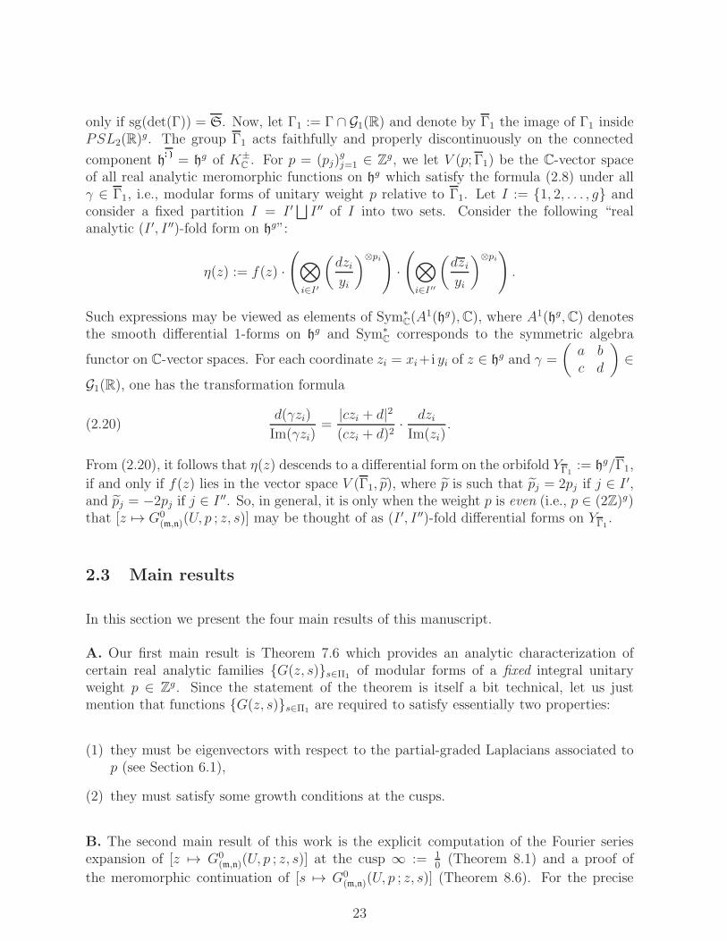
of all real analytic meromorphic functions on hg which satisfy the formula (2.8) under allγ ∈ Γ1, i.e., modular forms of unitary weight p relative to Γ1. Let I := 1, 2, . . . , g andconsider a fixed partition I = I ′
⊔I ′′ of I into two sets. Consider the following “real
analytic (I ′, I ′′)-fold form on hg”:
η(z) := f(z) ·(⊗
i∈I′
(dziyi
)⊗pi)
·(⊗
i∈I′′
(dziyi
)⊗pi).
Such expressions may be viewed as elements of Sym∗C(A
1(hg),C), where A1(hg,C) denotesthe smooth differential 1-forms on hg and Sym∗
C corresponds to the symmetric algebra
functor on C-vector spaces. For each coordinate zi = xi+i yi of z ∈ hg and γ =
(a bc d
)∈
G1(R), one has the transformation formula
d(γzi)
Im(γzi)=
|czi + d|2(czi + d)2
· dziIm(zi)
.(2.20)
From (2.20), it follows that η(z) descends to a differential form on the orbifold YΓ1:= hg/Γ1,
if and only if f(z) lies in the vector space V (Γ1, p), where p is such that pj = 2pj if j ∈ I ′,and pj = −2pj if j ∈ I ′′. So, in general, it is only when the weight p is even (i.e., p ∈ (2Z)g)that [z 7→ G0
(m,n)(U, p ; z, s)] may be thought of as (I ′, I ′′)-fold differential forms on YΓ1.
2.3 Main results
In this section we present the four main results of this manuscript.
A. Our first main result is Theorem 7.6 which provides an analytic characterization ofcertain real analytic families G(z, s)s∈Π1 of modular forms of a fixed integral unitaryweight p ∈ Zg. Since the statement of the theorem is itself a bit technical, let us justmention that functions G(z, s)s∈Π1 are required to satisfy essentially two properties:
(1) they must be eigenvectors with respect to the partial-graded Laplacians associated top (see Section 6.1),
(2) they must satisfy some growth conditions at the cusps.
B. The second main result of this work is the explicit computation of the Fourier seriesexpansion of [z 7→ G0
(m,n)(U, p ; z, s)] at the cusp ∞ := 10(Theorem 8.1) and a proof of
the meromorphic continuation of [s 7→ G0(m,n)(U, p ; z, s)] (Theorem 8.6). For the precise
23
meaning of the Fourier series expansion at a cusp c ∈ P1(K) we refer the reader to Section5.5. The non-constant Fourier coefficients of G0
(m,n)(U, p ; z, s) can be written in terms of the
Tricomi’s confluent hypergeometric function (see equations (3.5) and (3.8) for the precisedefinitions) that was considered in [34]. On the other hand, the constant term of theFourier series expansion of G0
(m,n)(U, p ; z, s), at the cusp ∞, can be written in terms of a
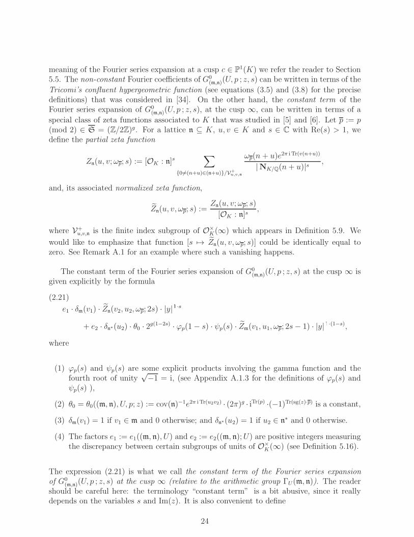
special class of zeta functions associated to K that was studied in [5] and [6]. Let p := p(mod 2) ∈ S = (Z/2Z)g. For a lattice n ⊆ K, u, v ∈ K and s ∈ C with Re(s) > 1, wedefine the partial zeta function
Zn(u, v;ωp; s) := [OK : n]s∑
06=(n+u)∈(n+u)/V+u,v,n
ωp(n + u)e2π i Tr(v(n+u))
|NK/Q(n+ u)|s ,
and, its associated normalized zeta function,
Zn(u, v, ωp; s) :=Zn(u, v;ωp; s)
[OK : n]s,
where V+u,v,n is the finite index subgroup of O×
K(∞) which appears in Definition 5.9. We
would like to emphasize that function [s 7→ Zn(u, v, ωp; s)] could be identically equal tozero. See Remark A.1 for an example where such a vanishing happens.
The constant term of the Fourier series expansion of G0(m,n)(U, p ; z, s) at the cusp ∞ is
(1) ϕp(s) and ψp(s) are some explicit products involving the gamma function and thefourth root of unity
√−1 = i, (see Appendix A.1.3 for the definitions of ϕp(s) and
ψp(s) ),
(2) θ0 = θ0((m, n), U, p; z) := cov(n)−1e2π i Tr(u2v2) · (2π)g · iTr(p) ·(−1)Tr(sg(z)·p) is a constant,
(3) δm(v1) = 1 if v1 ∈ m and 0 otherwise; and δn∗(u2) = 1 if u2 ∈ n∗ and 0 otherwise.
(4) The factors e1 := e1((m, n), U) and e2 := e2((m, n);U) are positive integers measuringthe discrepancy between certain subgroups of units of O×
K(∞) (see Definition 5.16).
The expression (2.21) is what we call the constant term of the Fourier series expansionof G0
(m,n)(U, p ; z, s) at the cusp ∞ (relative to the arithmetic group ΓU(m, n)). The readershould be careful here: the terminology “constant term” is a bit abusive, since it reallydepends on the variables s and Im(z). It is also convenient to define
Remark 2.19. When s ∈ Π1 is fixed, one may think of the expression [∞; s]-part-G0(m,n)(U, p ; z, s)
as being the obstruction for the function [z 7→ G0(m,n)(U, p ; z, s)] to be square-integrable at
the cusp ∞, in the sense of Definition 5.38.
We would like to emphasize here that the function ψp(s) and ϕp(s) only depend on theweight parameter p ∈ Zg and not on the data U,m, n. Moreover, the expression ψp(s) de-pends only on p ∈ S rather than p itself. Therefore, it is legitimate to write ψp(s). However,the function ϕp(s) really depends on p itself and not just on p. It follows from these obser-vations, that the constant term of the Fourier series expansion of [z 7→ G0
(m,n)(U, p ; z, s)],
up to the function ϕp(s), “only sees” the weight p modulo 2.
Remark 2.20. From (2.21), it follows from the definitions of δm(v1) and δn∗(u2) that theconstant term of the Fourier series of G0
(m,n)(U, p ; z, s) at the cusp ∞ vanishes identically
in the variables s and Im(z), if v1 /∈ m and u2 /∈ n∗.
Remark 2.21. Let q ∈ S. If we replace z by zq in (2.21), then the second term of (2.21)gets multiplied by (−1)Tr(q·p). It follows from this observation that, up to the sign, thedependence of θ0((m, n), U, p; z) on z is only a dependence on sg(z) = sg(y).
Let u, v ∈ K×. In Appendices A.1 and A.1.1, it is explained how a previous result ofthe author, proved in [5], implies that
Zn(u, v, ωp; s) = cov(n∗) · e2π i TrK/Q(uv) · λp(1− s) · Zn∗(−v, u, ωp; 1− s),(2.22)
for some explicit function λp(s), where p ∈ S. Note that since
the functional equation (2.22) implies the symmetry
λp(1− s) = (−1)Tr(p)λp(s)−1.(2.24)
For an integral weight p ∈ Zg, it is convenient to define λp(s) := λp(s). It is explained inAppendix A.1.3, that the following relations hold true
(1.a) ϕp(1− s) = (−1)Tr(p) · ϕp(s)−1,
(2.a) ϕ−p(s) = ϕp(s),
(3.a) ψp(s) · (2π)2g(1−s) = λp(2s− 1).
(4.a) ϕp(1− s) · ψp(s) =∏g
j=1Γ(2s−1)
Γ(s−pj/2)Γ(s+pj/2) .
25
C. The third main result of this work (see Theorem 9.10 below) is a proof of a functional
equation for the completed Eisenstein series G0m,n(U, p ; z, s) (see Section 9.1 for the precise
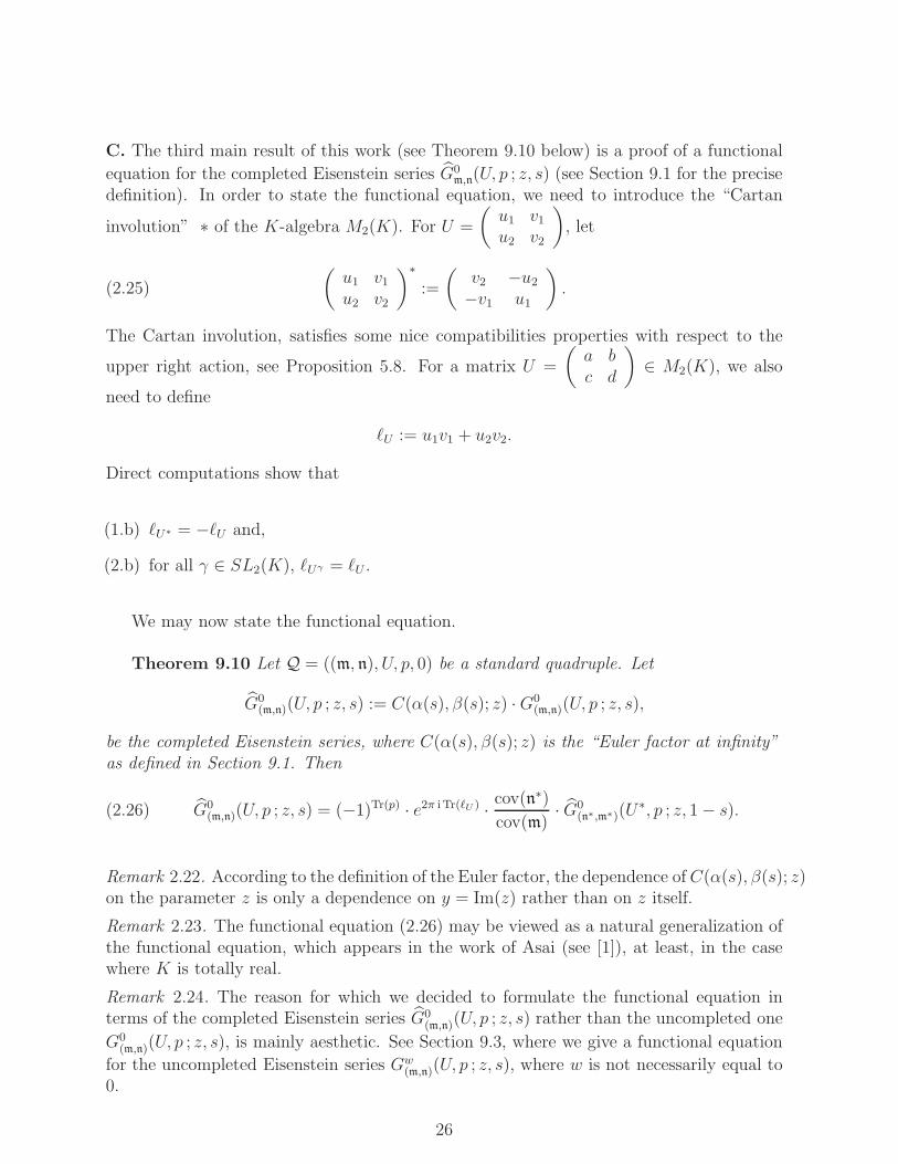
definition). In order to state the functional equation, we need to introduce the “Cartan
involution” ∗ of the K-algebra M2(K). For U =
(u1 v1u2 v2
), let
(u1 v1u2 v2
)∗:=
(v2 −u2−v1 u1
).(2.25)
The Cartan involution, satisfies some nice compatibilities properties with respect to the
upper right action, see Proposition 5.8. For a matrix U =
(a bc d
)∈ M2(K), we also
need to define
ℓU := u1v1 + u2v2.
Direct computations show that
(1.b) ℓU∗ = −ℓU and,
(2.b) for all γ ∈ SL2(K), ℓUγ = ℓU .
We may now state the functional equation.
Theorem 9.10 Let Q = ((m, n), U, p, 0) be a standard quadruple. Let
G0(m,n)(U, p ; z, s) := C(α(s), β(s); z) ·G0
(m,n)(U, p ; z, s),
be the completed Eisenstein series, where C(α(s), β(s); z) is the “Euler factor at infinity”as defined in Section 9.1. Then
G0(m,n)(U, p ; z, s) = (−1)Tr(p) · e2π i Tr(ℓU ) · cov(n
∗)
cov(m)· G0
(n∗,m∗)(U∗, p ; z, 1− s).(2.26)
Remark 2.22. According to the definition of the Euler factor, the dependence of C(α(s), β(s); z)on the parameter z is only a dependence on y = Im(z) rather than on z itself.
Remark 2.23. The functional equation (2.26) may be viewed as a natural generalization ofthe functional equation, which appears in the work of Asai (see [1]), at least, in the casewhere K is totally real.
Remark 2.24. The reason for which we decided to formulate the functional equation interms of the completed Eisenstein series G0
(m,n)(U, p ; z, s) rather than the uncompleted one
G0(m,n)(U, p ; z, s), is mainly aesthetic. See Section 9.3, where we give a functional equation
for the uncompleted Eisenstein series Gw(m,n)(U, p ; z, s), where w is not necessarily equal to
0.
26
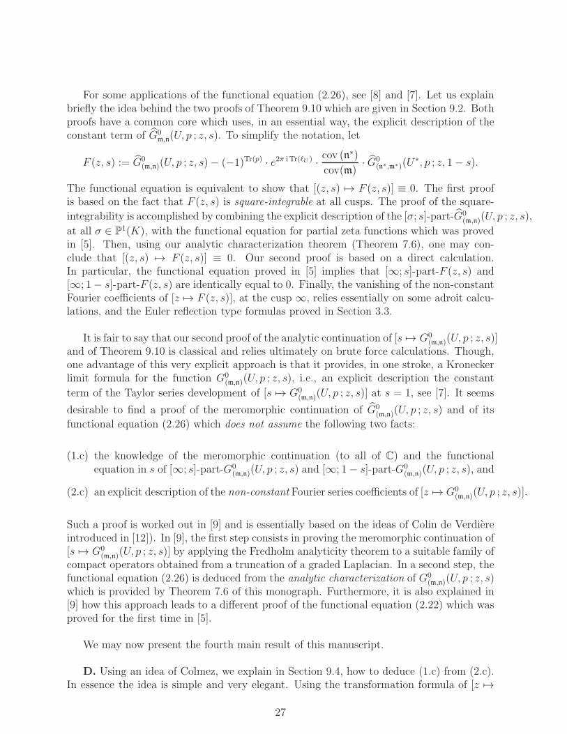
For some applications of the functional equation (2.26), see [8] and [7]. Let us explainbriefly the idea behind the two proofs of Theorem 9.10 which are given in Section 9.2. Bothproofs have a common core which uses, in an essential way, the explicit description of theconstant term of G0
m,n(U, p ; z, s). To simplify the notation, let
F (z, s) := G0(m,n)(U, p ; z, s)− (−1)Tr(p) · e2π i Tr(ℓU ) · cov (n
∗)
cov(m)· G0
(n∗,m∗)(U∗, p ; z, 1− s).
The functional equation is equivalent to show that [(z, s) 7→ F (z, s)] ≡ 0. The first proofis based on the fact that F (z, s) is square-integrable at all cusps. The proof of the square-
integrability is accomplished by combining the explicit description of the [σ; s]-part-G0(m,n)(U, p ; z, s),
at all σ ∈ P1(K), with the functional equation for partial zeta functions which was provedin [5]. Then, using our analytic characterization theorem (Theorem 7.6), one may con-clude that [(z, s) 7→ F (z, s)] ≡ 0. Our second proof is based on a direct calculation.In particular, the functional equation proved in [5] implies that [∞; s]-part-F (z, s) and[∞; 1− s]-part-F (z, s) are identically equal to 0. Finally, the vanishing of the non-constantFourier coefficients of [z 7→ F (z, s)], at the cusp ∞, relies essentially on some adroit calcu-lations, and the Euler reflection type formulas proved in Section 3.3.
It is fair to say that our second proof of the analytic continuation of [s 7→ G0(m,n)(U, p ; z, s)]
and of Theorem 9.10 is classical and relies ultimately on brute force calculations. Though,one advantage of this very explicit approach is that it provides, in one stroke, a Kroneckerlimit formula for the function G0
(m,n)(U, p ; z, s), i.e., an explicit description the constant
term of the Taylor series development of [s 7→ G0(m,n)(U, p ; z, s)] at s = 1, see [7]. It seems
desirable to find a proof of the meromorphic continuation of G0(m,n)(U, p ; z, s) and of its
functional equation (2.26) which does not assume the following two facts:
(1.c) the knowledge of the meromorphic continuation (to all of C) and the functionalequation in s of [∞; s]-part-G0
(m,n)(U, p ; z, s) and [∞; 1− s]-part-G0(m,n)(U, p ; z, s), and
(2.c) an explicit description of the non-constant Fourier series coefficients of [z 7→ G0(m,n)(U, p ; z, s)].
Such a proof is worked out in [9] and is essentially based on the ideas of Colin de Verdiereintroduced in [12]). In [9], the first step consists in proving the meromorphic continuation of[s 7→ G0
(m,n)(U, p ; z, s)] by applying the Fredholm analyticity theorem to a suitable family ofcompact operators obtained from a truncation of a graded Laplacian. In a second step, thefunctional equation (2.26) is deduced from the analytic characterization of G0
(m,n)(U, p ; z, s)which is provided by Theorem 7.6 of this monograph. Furthermore, it is also explained in[9] how this approach leads to a different proof of the functional equation (2.22) which wasproved for the first time in [5].
We may now present the fourth main result of this manuscript.
D. Using an idea of Colmez, we explain in Section 9.4, how to deduce (1.c) from (2.c).In essence the idea is simple and very elegant. Using the transformation formula of [z 7→
27
G0(m,n)(U, p ; z, s)] (see Proposition 5.23) under the matrix γ =
(0 1−1 0
), one shows that
a certain three-term linear combination of partial zeta functions equals to an infinite linearcombination of the non-constant Fourier series coefficients aξ(y, s)ξ 6=0 of the function[x 7→ G0
(m,n)(U, p ; x + i y, s)]. Moreover, from the explicit description of aξ(y, s)ξ 6=0, we
know that the functions [s 7→ aξ(y, s)] must satisfy a certain functional equation in thevariable s. Finally, using some linear algebra, one may transfer this functional equation toone of the partial zeta functions which appears in the original three-term linear combination.
2.4 Relationships between Gw(m,n)(U, p ; z, s)with some GL2-Eisenstein
series appearing in the literature
We would like now to discuss briefly the relationships between the GL2-Eisenstein series ofthis manuscript and the GL2-Eisenstein series appearing in the literature. For w ≥ 3, oneeasily sees that
Fw(U ; z) := Gw(m,n)(U, O; z, s)|s=0,(2.27)
is a holomorphic Eisenstein series of parallel weight w. The restriction w ≥ 3 (so thatw2> 1) is imposed so that the series, on the right-hand side of (2.27), converges absolutely
(however see Remark 8.11 for the case w = 2). In Section 8.3, the Fourier series expansionof [z 7→ Fw(U ; z)] is given. In the special case where the parameter matrix U has the
form
(0 v10 v2
), the Eisenstein series Fw(U ; z) are essentially the holomorphic Eisenstein
constructed by Deligne and Ribet in [13], see p. 269. From the perspective of [13], theusefulness of these Eisenstein series comes from the fact that, for a finite sum of these(of possibly different weights), one may apply, under some assumptions, the so-called “q-expansion principle” in order to obtain non-trivial p-adic congruences for the constant termof its Fourier series at the various cusps. From these p-adic congruences, it is then possibleto construct p-adic L-functions.
When p ∈ Zg and u1 = u2 = 0, w ∈ Z, and m = n = ax the (uncompleted) real analyticEisenstein series
were considered by Shimura (see (2.2) of [31]). Here, x ⊆ K is a fractional ideal and a ⊆ Kis an integral ideal. From the perspective of [31], the interest for such Eisenstein seriescomes from the fact that their special values, when s = 0 and z ∈ hg is a CM point,are algebraic numbers multiplied by some transcendental period which depends only onk and p and not on the CM point z and the parameter matrix U . As it is explained in[31], such a result may be used to show that special values of L-functions associated toa Grossencharacter ψ of type A0 (in the sense of Weil) are equal to an algebraic numbertimes a period which depends only on the infinity type of ψ.
28
3 Some formulas
In this section we introduce various functions which are required in order to write downexplicit formulas for the non-zero Fourier coefficients of our Eisenstein series. It will alsobe important for us to study the meromorphic continuation of these functions on certaindomains and also give some growth estimates when the parameters vary in certain regions.
Let α and β be complex numbers and view z = x + i y as a variable in h±. We definethe formal sum
f(α, β; z) :=∑
n∈Z(z + n)−α(z + n)−β,(3.1)
When Re(α + β) > 1, the sum above is absolutely convergent. Note that the continuousfunction [x 7→ f(α, β; x + i y)] is invariant under translation by 1. Therefore, one mayconsider its Fourier series expansion, namely
f(α, β; z) :=∑
n∈Zρn(y, α, β)e
2π inx,(3.2)
where the Fourier coefficients are given by the formulas
ρn(α, β; y) =
∫ 1
0
f(α, β; z)e−2π inxdx
=
∫ ∞
−∞z−α(z)−βe−2π inxdx.(3.3)
The second equality is justified from the absolute convergence of (3.1) which allows oneto interchange the order of summation with the integral. We note that the integral in(3.3) converges absolutely, since Re(α + β) > 1. Because x 7→ f(α, β, x + i y) is a realanalytic function on the one-dimensional torus R/Z, we know, from (1) of Theorem 4.10in Section 4.2, that the Fourier series (3.2) converges absolutely, and that for all z ∈ h±,
f(α, β; z) = f(α, β; z). In particular, the Fourier series computes the value of f(α, β; z).Moreover, from (3) of Theorem 4.10, we also know that there exists a positive constantD ∈ R>0 (depending on y), such that |ρn(α, β, y)| ≤ e−D|n| for all n ∈ Z.
Following Shimura (see p. 84 of [32]), for z = x + i y ∈ h±, t ∈ R and α, β ∈ C withRe(α + β) > 1, we define
τ(α, β; t, y) :=
∫ ∞
−∞z−α(z)−βe−2π itxdx.(3.4)
Note that this integral is absolutely convergent. Later on, a more precise inequality of theform |τ(α, β; t, y)| ≤ Cs|t|Re(α)+Re(β)−1e−2π|ty|, as |ty| → ∞ will be proved (see Proposition3.15). The integral (3.4) satisfies some obvious symmetries: For all t, y, a ∈ R×, we havethe following rules:
29
(i) τ(α, β; t,−y) = τ(β, α; t, y)
(ii) τ(α, β; t, y) = τ(β, α;−t, y) (here the “bar” denotes the complex conjugation)
(iii) If y ∈ R× and a > 0 then τ(α, β; at, y) = |a|α+β−1τ(α, β; t, ay).
(iv) If y ∈ R>0 and a < 0 then τ(α, β; at, y) = eπ i(β−α)|a|α+β−1τ(α, β; t, ay).
(v) If y ∈ R<0 and a < 0 then τ(α, β; at, y) = eπ i(α−β)|a|α+β−1τ(α, β; t, ay).
All the proofs of these formulas are straightforward. Let us just point out that the rules(iv) and (v) follow from the formulas (az)α = |a|αzαe−απ i when z ∈ h+, a ∈ R<0; and(az)α = |a|αzαeαπ i when z ∈ h−, a ∈ R<0. These last two formulas follow from the productrule (2.2).
It will be important for us to give explicit formulas for τ(α, β; t, y) in the following twocases:
(a) Re(α),Re(β) > 0 and Re(α + β) > 1.
(b) α ∈ Z≥2 and β = 0 (from the rule (ii) one automatically obtains the formula for thecase where β ∈ Z≥2 and α = 0),
Remark 3.1. Note that these two cases do not overlap, but (b) may be viewed as a limitingcase of (a), as β → 0+ and α ∈ Z≥2. From the perspective of Eisenstein series, this laterobservation means that holomorphic Eisenstein series can be viewed as a limit (in the svariable) of real analytic Eisenstein series. Explicit formulas in the case (b) (see below) willbe used in Section 8.3 to compute the Fourier coefficients of holomorphic Eisenstein series.
We first focus on obtaining explicit formulas for the case (a). Explicit formulas for the case(b) will be given in Proposition 3.16.
On page 366 of [34], Siegel introduced the confluent hypergeometric function σ(y;α, β),given by
σ(y;α, β) :=
∫ ∞
0
(u+ 1)α−1uβ−1e−yudu,(3.5)
where y ∈ R>0, Re(β) > 0 and α is any complex number. This allowed Siegel to obtainan explicit formula for τ(α, β;n, y) (n ∈ Z) in terms of σ(y;α, β). On p. 84 of [32], Siegelstates (without a proof) the following explicit formulas for the τ( , ; , ) in terms of theσ( ; , ) function.
30
Lemma 3.2. Let α, β ∈ C be such that Re(α) > 0,Re(β) > 0 and Re(α + β) > 1. Lett ∈ R and y ∈ R×. Then we have:
τ(α, β; t, y)
=
(2π)α+β iβ−α |t|α+β−1Γ(α)−1Γ(β)−1e−2π|ty|σ(4π|ty|;α, β) if y > 0, t > 0,
(2π)α+β iα−β |t|α+β−1Γ(α)−1Γ(β)−1e−2π|ty|σ(4π|ty|; β, α) if y < 0, t > 0,
(2π)α+β iβ−α |t|α+β−1Γ(α)−1Γ(β)−1e−2π|ty|σ(4π|ty|; β, α) if y > 0, t < 0,
(2π)α+β iα−β |t|α+β−1Γ(α)−1Γ(β)−1e−2π|ty|σ(4π|ty|;α, β) if y < 0, t < 0,
(2π) · iβ−α Γ(α+β−1)Γ(α)Γ(β)
(2y)1−α−β if t = 0, y > 0,
(2π) · iα−β Γ(α+β−1)Γ(α)Γ(β)
(2|y|)1−α−β if t = 0, y < 0,
where Γ(x) stands for the gamma function evaluated at x.
Proof For a proof of Lemma 3.2, see the proof of Lemma 1 of [32].
Remark 3.3. Note that the rules (i), (ii), (iii), (iv) and (v) for the function τ( , ; , ) canall be verified directly from the above list of formulas.
Remark 3.4. Later on, it will be explained (see Corollary 3.14) that the function (y, α, β) 7→σ(y;α, β) admits a single-valued meromorphic continuation when the triple (y, α, β) variesover the domain C\R≤0 × C× C.
It also will be convenient for us to introduce a modified version of the function τ(α, β; t, y)that satisfies additional symmetry relations.
Definition 3.5. Let α, β ∈ C\Z≤0, t ∈ R× and z = x+ i y ∈ h±. We set
p(α, β; t, y) :=
iǫ(y)(α−β) Γ(α)(4π|ty|)β if ty > 0,
iǫ(y)(α−β) Γ(β)(4π|ty|)α if ty < 0,(3.6)
where ǫ(y) = sign(y). We defined the “completed τ -function” as
Remark 3.6. We note that the functions p(α, β; t, y) and τ (α, β; t, y) depend only on thetriple (α, β, ty) rather than the quadruple (α, β, t, y) itself. Moreover, the definition ofp(α, β; t, y) is such that the positions of α and β, on the right-hand side of (3.6), areinterchanged, according to the sign of ty.
The next formulas are easy to prove.
Proposition 3.7. Let α, β ∈ C\Z≤0 and let t, y, a ∈ R×. Then the following identitieshold true:
31
(1) If a > 0, p(α, β; at, y) = p(α, β; t, ay).
(2) Assume that α−β ∈ Z. Then, if a < 0, we have p(α, β; at, y) = (−1)α−β ·p(α, β; t, ay).
A priori, the function y 7→ τ(α, β; 1, y) (see (3.4)) is only defined for y ∈ R×, α, β ∈ C withRe(α) > 0, Re(β) > 0 and Re(α + β) > 1. In order to to give a meaning to τ(α, β; 1, y),when (α, β, y) lies outside this region, we will express Siegel’s confluent hypergeometricfunction (σ( ; , )) in terms of Tricomi’s confluent hypergeometric function (U( , ; )). Inthis way, we can take advantage of the extensive study of U( , ; ) which was done in [36].In particular, this allows us to transfer the various analytic properties of U( , ; ) to σ( ; , )and to τ(α, β; 1, y).
We first define U( , ; ) in terms of σ( ; , ). Then, we present some of the propertiesof U( , ; ) that will be needed in the sequel. Let α, β ∈ C with Re(β) > 0 and set a := β,b := α + β. For any t ∈ R>0, Tricomi’s confluent hypergeometric function (cf. 3.1.19 of[36]) is defined as
U(a, b; t) :=1
Γ(a)σ(t; b− a, a),(3.8)
or equivalently,
U(β, α+ β; t) :=1
Γ(β)σ(t;α, β).(3.9)
32
One may verify that U(a, b; t) satisfies the Kummer’s hypergeometric differential equation
td2w
dt2+ (b− t)
dw
dt− a · w = 0,(3.10)
which has a regular singular point at t = 0 and an irregular singular point at t = ∞. Notethat the differential equation (3.10) is a degenerate form of the usual Gauss’ hypergeometricequation, given by
t(1− t)d2w
dt2+ [b− (a+ c+ 1)t]
dw
dt− ac · w = 0.(3.11)
If one replaces t by tcin (3.11) (so dw
dtgoes to cdw
dtand d2w
dt2goes to c2 d
2wd2t
) and if one letsc→ ∞, we obtain the ODE (3.10).
The next proposition describes some properties of the function U(a, b; t).
Proposition 3.8. (1) The function (a, b, z) 7→ U(a, b; z) admits a multi-valued analyticcontinuation to all of C××C× C\0.
(2) Let z ∈ C\0 be fixed. Then, function (a, b) 7→ U(a, b; z) admits a single-valuedanalytic continuation to all of C× C.
(3) Let L ⊆ C be a half-line joining 0 to ∞. Then, the function (a, b, z) 7→ U(a, b; z)admits an holomorphic extension to C× C× (C\L).
(4) Let L ⊆ C be a half-line joining 0 to ∞. Let a, b ∈ C, with Re(a),Re(b) > 0 be fixed.Then, the one variable holomorphic function z 7→ U(b, a + b; z) is non-constant.
(5) For a, b ∈ C fixed, we have U(a, b; z) ∼ z−a(1 +O(|z|−1)) as Re(z) → ∞. In particu-lar, if Re(a) > 0, we have the asymptotic U(a, b; z) ∼ z−a as Re(z) → ∞. Moreover,if Re(a) > 0, U(a, b; z) is the unique solution of the linear ODE (3.11), which is, upto a multiplicative scalar, bounded as Re(z) → ∞.
(6) For all β ∈ R>0, α ∈ R and y ∈ R>0, we have U(β, α+ β; y) > 0.
(7) For all b ∈ C and z ∈ C\0, we have U(0, b; z) = 1.
(8) U(a, a + 1; z) = 1za.
(9) Let α, β ∈ C and z ∈ C\0. Then, the quantity zβ ·U(β, α+β; z) is invariant underthe substitution α 7→ 1− β and β 7→ 1− α.
(10) ddzU(a, b; z) = −aU(a + 1, b+ 1, z).
Remark 3.9. Note that in the last statement of (5), we could have replaced “which isbounded as Re(z) → ∞” by “which is bounded by |N(y)|N for some positive integerN ∈ Z≥1, as Re(z) → ∞”.
33
Proof Let 1F1(a,b;z)Γ(b)
be the normalized Kummer series. It follows from the equation
(1.3.5) on page 5 of [36] that (a, b, z) 7→ 1F1(a,b;z)Γ(b)
is a holomorphic function on all of C3.
Equation (1.3.1) in [36] reads as
U(a, b; z) =Γ(1− b)
Γ(1 + a− b)1F1(a, b; z) +
Γ(b− 1)
Γ(a)x1−b1F1(1 + a− b, 2− b; z).(3.12)
It is valid, a priori, for all (a, b, z) ∈ C3 with b /∈ Z≤0. In order to handle the case whereb ∈ Z≤0, one may look at Equation (1.3.5) of [36] which reads as
U(a, b; z) =π
sin(πb)
(1F1(a, b; z)
Γ(1 + a− b)Γ(b)− x1−b1F1(1 + a− b, 2− b; z)
Γ(a)Γ(2− b)
).(3.13)
Note that (3.13) makes sense when n ∈ Z≤0 and b→ n. From these two equations, we seethat (a, b, z) 7→ U(a, b; z) becomes a multi-valued function on C××C×C\0. The fact theU(a, b; z) is multi-valued comes from the need of fixing a branch of z 7→ z1−b. This proves(1). In particular, if z ∈ C\0 is fixed, the function (a, b) 7→ U(a, b; z) is single-valued onall of C2. This proves (2).
The proof of (3) follows directly from Equations (3.13) and (3.12).
Let us prove (4). Let a, b ∈ C with Re(a),Re(b) > 0. We do a proof by contradiction.Assume that for all z ∈ C\L, z 7→ U(b, a + b; z) = 0. Then
limz→0
z1−a−b ·(za+b−1 · U(b, a + b; z)
)= 0.(3.14)
But from (2) of Proposition 3.11 (see the proposition below), the limit on the left handside of (3.14) is equal to
limz→0
z1−a−b · Γ(a+ b− 1)
Γ(b).(3.15)
From the infinite product of 1Γ(z)
, we know that Γ(z) 6= 0 for all z ∈ C. Therefore, since
Re(a),Re(b) > 0, the quotient Γ(a+b−1)Γ(b)
is either equal to ∞ (if a + b − 1 = 0) or different
from 0. But this is absurd, since the limit in (3.14) is equal to 0 and the limit in (3.15) isequal to ∞. This concludes the proof of (4).
For a proof of (5), see pages 58-60 of [36].
The proof of (6) follows directly from the integral (3.5) and the identity (3.8).
Let us prove (7). When b /∈ Z≤0, (7) follows from equation (3.12) and the observationthat for all c ∈ C\Z≤0, 1F1(0, c; z) = 1. If b ∈ Z≤0, then one uses instead equation (3.13).This proves (6).
The proof of (8) follows from (3.5) and (3.8).
34
The proof of (9) follows from equation (1.4.9) on page 6 of [36].
For a proof of (10), one may simply differentiate the expression in (3.5) under theintegral sign to find the relation d
Remark 3.10. It follows from the proof of (1) of Proposition 3.8 that for any half-line L, inthe complex plane, joining 0 to ∞, the function (a, b, z) 7→ U(a, b; z) admits a single-valuedholomorphic continuation to all of C× C× (C\L).
The next proposition gives the limit values of the function z 7→ U(β, α + β; z) whenz → 0, and when the complex parameters (α, β) lie in certain regions of C2. These twolimit formulas will be used later on.
Proposition 3.11. (1) Assume that Re(α+ β) < 1, then
limz→0
U(β, α+ β; z) =Γ(1− (α + β))
Γ(1− α).
(2) Assume that Re(α + β) > 1, then
limz→0
zα+β−1 · U(β, α + β; z) =Γ(α + β − 1)
Γ(β).
Proof The proof of (1) and (2) follow from the equations (3.12) and (3.13) and theobservation that, for all (α, β) ∈ C2,
limz→0
1F1(α, β; z)
Γ(β)= 1.
Remark 3.12. Note that the two sets (α, β) ∈ Cg : Re(α + β) < 1 and (α, β) ∈ Cg :Re(α + β) > 1. don’t overlap.
3.1.1 Relationship between U(a, b; z) and Ks(z)
In many papers related to the computation of the Fourier series expansion GL2-real ana-lytic Eisenstein series, the K-Bessel function (or sometimes also called the modified Besselfunction of the second kind) appears. In this short section, we explain the relationshipbetween the K-Bessel function and Tricomi’s confluent hypergeometric function U( ; , ).
For z ∈ C with Re(z) > 0, one may define the K-Bessel function using its Schlafi’sintegral representation as
Ks(z) :=
∫ ∞
0
e−z cosh(t) cosh(st)dt
=1
2
∫ ∞
0
e−12z(u+1/u)(us + u−s)
du
u,(3.16)
35
where u = et. From equation (1.8.7) of [36], we have
U(s, 2s; 2z) =(2z)
12−s
√π
ezKs− 12(z).(3.17)
Remark 3.13. If we define
Ks(z) :=1
2
∫ ∞
0
e−12z(u+1/u)us
du
u,
then Ks(z) is invariant under the change of variable u 7→ 1u. Therefore, Ks(z) = K−s(z).
Looking at (3.16), we obtain the relation Ks(z) = 2Ks(z). For this reason, some authors
also define the K-Bessel function by Ks(z) rather than Ks(z).
3.2 Meromorphic continuation of some functions
In this section we prove the meromorphic continuation of various functions which have beenintroduced before. Ultimately, the existence of such meromorphic continuations boil downto the analytic properties of the Tricomi’s confluent hypergeometric functions [(a, b, z) 7→U(a, b; z)] and of the gamma function Γ(z).
Let z ∈ C\0 be fixed. From Proposition 3.8, we know that the function (a, b) 7→U(a, b; z) admits a holomorphic continuation to all of C2. Looking at the identity (3.8)and using the well-known properties of the gamma function, we obtain immediately thefollowing corollary:
Corollary 3.14. Let t ∈ R\0 be fixed. Then, function (α, β) 7→ σ(t;α, β) admits asingle-valued meromorphic continuation to all of C2. Moreover, it is analytic on the domainC× C\Z≤0. For a fixed pair (t, α) ∈ (R\0)× C, the one variable meromorphic functionβ 7→ σ(t, α, β) is holomorphic on all of C\Z≤0, with possible poles of order at most one atthe elements in Z≤0.
Having obtained the meromorphic continuation of σ(t;α, β), we now focus on the τ -function, i.e., τ(α, β; t, y) (see (3.4)). Let t, y ∈ R\0 be fixed. To fix the idea, let usassume that t, y > 0. From Lemma 3.2 and equation (3.8), we have
Recall that α 7→ Γ(α) is a holomorphic function on all ofC. We decide to extend analyticallythe function (α, β) 7→ τ(α, β; t, y) to all (α, β) ∈ C×C, using the right-hand side of (3.18).In a similar way, we may also define an analytic continuation of (α, β) 7→ τ(α, β; t, y), to allof C2, when the pair (t, y) is such that (sign(t), sign(y))) ∈ (−1,+1), (+1,−1), (−1,−1).
We thus have
36
Proposition 3.15. Let t, y ∈ R\0 be fixed. Then the function [(α, β) 7→ τ(α, β; t, y)]admits an analytic continuation to all of C2. If ty > 0, and α ∈ Z≤0 then [(t, y) 7→τ(α, β; t, y)] ≡ 0. If ty < 0, and β ∈ Z≤0 then [(t, y) 7→ τ(α, β; t, y)] ≡ 0. Assume thatRe(α) > 0 and Re(β) > 0. Then, there exists a positive constant Cs > 0, such that for allt, y ∈ R\0 with (sign(t), sign(y)) fixed, we have that
Proof The first three claims follow from the definition of τ(α, β; t, y) and (2) of Propo-sition 3.8. The proof of (3.19) follows from the asymptotic formula for U(β, α+ β; z) (andU(α, α + β; z)) given in (5) of Proposition 3.8 and the explicit formula of τ(α, β; t, y) interms of U( , ; ).
We may now give the explicit formula for τ(α, β; t, y) when α ∈ Z≥2 and β = 0 (case(b) in Section 3).
Proposition 3.16. Let t ∈ R× and z = x + i y ∈ h±. Let α ∈ Z≥2 and set ǫ = sign(y).Then
τ(α, 0; t, y) =
(−ǫ · 2π i)α |t|α−1
(α−1)!e−2π|ty| if sign(ty) > 0
0 if sign(ty) < 0
and
τ(0, α; t, y) =
0 if sign(ty) > 0,
(ǫ · 2π i)α |t|α−1
(α−1)!e−2π|ty| if sign(ty) < 0.
Proof Let t, y ∈ R× be fixed. In virtue of the principle of identity for holomorphicfunctions in many variables, it follows from Proposition 3.15 that the first 4 formulas givenin Lemma 3.2, hold true for all α, β ∈ C. Finally, a direct computation involving each ofthese four cases, combined with (4) of Proposition 3.8, give the formulas above.
In a similar way, for a fixed pair t, y ∈ R\0, we may extend the definition of (α, β) 7→τ(α, β; t, y) (see Definition 3.5) to all C2. To fix the idea, let us assume that t, y > 0. Then,from the definition of τ( , ; , ), we have
In particular, (α, β) 7→ τ (α, β; t, y) admits an holomorphic continuation to all of C2. Simi-larly, one may check that for each of the remaining three possibilities of (sign(t), sign(y)),the function (α, β) 7→ τ(α, β; t, y) is again holomorphic on all of C2. We thus obtain:
Proposition 3.17. Let t, y ∈ R\0 be fixed. Then, function (α, β, z) 7→ τ(α, β; t, y)admits an holomorphic continuation to all of C2.
37
3.3 Reflection formulas
The next two lemmas are the key to show that the non-constant terms of the Fourierseries expansion of the completed Eisenstein series G0
m,n(U, p ; z, s) (see Definition 9.1) areinvariant under the substitution s 7→ 1− s.
Lemma 3.18. Let z ∈ C\0 be fixed. Then, the expression
zβ · U(β, α + β; z),(3.20)
is invariant under the transformation α 7→ 1− β and β 7→ 1− α.
Proof This is a direct consequence of (9) of Proposition 3.8. See also Lemma 2 of [32].
Corollary 3.19. Let t, y ∈ R×. Then the function τ(α, β; t, y) = τ (α, β; 1, ty) is invariantunder the transformation α 7→ 1− β and β 7→ 1− α.
Proof This follows from Lemma 3.2, Lemma 3.18 and the definition of τ(α, β, t, y).
We will also need the following reflection formula which involves the p( , ; , ) functionwhich appears in Definition 3.5.
Proposition 3.20. Let α, β ∈ C\Z. For t1, t2, y1, y2 ∈ R×, we define
q(α, β; t1, y1; t2, y2) :=p(β, α; t1, y1)
p(α, β; t2, y2).(3.21)
Then the expression q(α, β; t1, y1; t2, y2) satisfies the following functional equation:
Note the swap between the pairs (t1, y1) and (t2, y2) on the right-hand side of (3.22).
Proof The proof of (3.22) follows directly from the definition of p(α, β; t, y) and theEuler’s reflection formula for the gamma function. The proof of (3.23) follows from therules (4) and (5) of Proposition 3.7.
38
Corollary 3.21. Let α, β ∈ C\Z with α − β ∈ Z. Let d, y ∈ R×, then the expressionq(α, β; 1, dy; 1, y) satisfies the following functional equation:
q(α, β; 1, dy; 1, y) =
(−1)α−β · q(1− β, 1− α; 1, dy; 1, y) · |d|α+β−1 if d > 0
q(1− β, 1− α; 1, dy; 1, y) · |d|α+β−1 if d < 0(3.24)
Proof This follows directly from Proposition 3.20.
4 Lattices in number fields and Fourier series expan-
sion
4.1 Lattices in number fields
In this section, we decided to gather, for the convenience of the reader, some results aboutlattices in number fields which are not easily found in the literature. The main goal ofthis section is to clarify the relations between two operations on lattices which arise inthe setting of functional equations in number theory: the multiplicative inverse operationL 7→ L−1 and the dual operation L 7→ L∗ (with respect to the trace pairing). Thesetwo operations arise naturally when one writes down the functional equations of partialzeta functions and GL2-Eisenstein series. In the literature on GL2-Eisenstein series, someauthors preferred to use the former operation while others, the latter. In most papers onGL2-Eisenstein series and partial zeta functions, the authors usually restrict themselvesto working with lattices of K, which are also fractional OK-ideals. In this setting, it iseasy to move from one point of view to the other, since, if a ⊆ K is a fractional OK-ideal,then one has the well-known relation a∗ = a−1d−1
K . Here, d−1K stands for the inverse of the
different ideal of K. In the present work, we decided to work systematically and almostexclusively with the dual operation. Except for this section and the proof of Proposition5.15, the multiplicative inverse operation will not be used. Although the role played by themultiplicative inverse operation in our work is very small, we think that it is worthwhile tospend some time clarifying its relationship with the dual operation in order to have a theorywhich simultaneously encompasses both points of view and which works for all lattices ofK, not just those ones which are fractional OK-ideals. Since all the results in this sectionare valid for arbitrary number fields, for this section only, we let K be an arbitrary numberfield of degree g over Q.
Let L ⊆ K be a Z-lattice, i.e., a free Z-module of rank g. For two lattices L1,L2 ⊆ K,we define their product as
L1L2 =
n∑
i=1
ℓ1,iℓ2,i : ℓ1,i ∈ L1, ℓ2,i ∈ L2, n ∈ Z≥1
.
39
One may verify that L1L2 is again a lattice. Moreover, the product operation on latticesis associative.
4.1.1 O-properness
Let L ⊆ K be a lattice. We define
OL := λ ∈ K : λL ⊆ L,and call OL the multiplier ring of L (or the endomorphism ring of L). If O is an order ofK, such that O = OL, then we say that L is O-proper. So, by definition, for any latticeL, we always have that L is OL-proper.
4.1.2 The multiplicative inverse operation
We define the multiplicative inverse of L to be
L−1 := λ ∈ K : λL ⊆ OL.Note that, by definition, L−1 is always an OL-module and that LL−1 ⊆ OL. Since L−1
is an OL-module, it follows that that OL ⊆ OL−1 . From the previous inclusion, it followsthat L ⊆ (L−1)−1. As Example 4.1 below shows, the three inclusions above could be strictin general. The example below is inspired from an email exchange with Keith Conrad, whokindly pointed out to me Exercise 18 on page 94 of [3].
Example 4.1. Let θ ∈ Q be such that θ3 = 2 and consider the cubic field K := Q(θ). Wehave that OK = Z[θ]. Let R := Z+2θZ+2θ2Z. One may verify that R is an order of indexfour in OK . Consider the lattice M := 4Z + θZ + θ2Z ⊆ K. Then direct computations(which we leave to the reader) show that
(i) OM = R,
(ii) M2 = 2Z+ 2θZ+ θ2Z,
(iii) OM2 = OK ,
(iv) M−1 = 2Z+ 2θZ+ θ2Z = 2OK + θ2OK ,
(v) OM−1 = OK and (M−1)−1 = 12(2OK + θOK) =
12(2Z+ θZ+ θ2Z) % M,
(vi) MM−1 ⊆ 2OK $ R.
Example 4.1 is instructive since it shows that if L1,L2 ⊆ K are O-proper, then L1L2
is not necessarily O-proper. Moreover, the lattice M above is such that OM 6= OM−1
and M $ (M−1)−1. In particular, if LattK denotes the set of all lattices in K, then theapplication [−1] : LattK → LattK , given by L 7→ L−1 is not necessarily involutive.
40
4.1.3 O-invertibility
Let L ⊆ K be an O-module. By definition of OL, we have O ⊆ OL. We say that L isO-invertible, if there exists an O-module L′ ⊆ K such that LL′ = O. Since OL · LL′ ⊆LL′ = O and 1 ∈ LL′ = O, this implies that OL ⊆ O. Therefore, O = OL. Thus, ifL is an O-invertible module, it is automatically O-proper. The converse is not true ingeneral. Indeed, looking at Example 4.1, we have OM = R and MM−1 $ R = OM.Therefore, the OM-proper lattice M is not OM-invertible. For a further discussion on thediscrepancy between the O-invertibility and O-properness, see Remark 4.6. Let L ⊆ K bea lattice and assume that there exists an OL-module L′, such that LL′ = OL. Then sucha lattice L′ is necessarily unique; indeed, this follows directly from the commutativity andthe associativity of the product operation on lattices. Moreover, one may verify that L′
must be equal to L−1. It follows from the discussion above that
LL−1 = OL ⇐⇒ 1 ∈ LL−1 ⇐⇒ L is OL-invertible.
Finally, if L is OL-invertible, then one may also check that (L−1)−1 = L and that OL =OL−1 .
It is worthwhile to remind the reader of the following set of equivalences forO-invertibilitywhich will be used later on in the proof of Corollary 4.8.
Theorem 4.2. Let O ⊆ OK be an order and let L ⊆ K be a lattice, which is also anO-module. Then the following statements are equivalent:
(1) L is O-invertible.
(2) L is a projective O-module.
(3) L is a locally free O-module, i.e., for each non-zero prime ideal p ⊆ O, one has thatLp is a free Op-module.
Proof For a proof of this fact, the author may consult for example [26].
4.1.4 Conductor of an order and invertibility of prime ideals
Definition 4.3. The conductor of an order O ⊆ K is defined as
cond(O) = cO = x ∈ K : xOK ⊆ O.
One may check that cO is the largest integral OK-ideal which is included in O. Inparticular, cO is an integral O-ideal.
41
Let O ⊆ OK be a fixed order. An ideal a ⊆ O (i.e. a is an O-module) is called invertible(relative to O) if Oa = O. The next proposition gives a complete characterization of theinvertible prime ideals of O.
Theorem 4.4. A non-zero prime ideal p ⊆ O is O-invertible if and only if p is relativelyprime to cO, i.e., p+ cO = O.
Proof See Theorem 6.1 of [11].
Remark 4.5. Note that the “only if direction” in Theorem 4.4 is no longer true if p is notprime. For example, assume that cO $ OK and let c > 1 be the smallest integer inside cO.Then the O-ideal c · O is invertible (since it is principal) but it is not coprime to cO.
4.1.5 The dual operation
We would like now to recall some classical results about dual lattices with respect to thetrace pairing. For a lattice L ⊆ K, we define the dual lattice of L (with respect to thepairing (x, y) 7→ TrK/Q(xy)) by
L∗ := x ∈ K : TrK/Q(xℓ) ∈ Z for all ℓ ∈ L.
Note that the ∗ operation is contravariant on the partially ordered set of lattices, i.e., ifL1 ⊆ L2, then L∗
1 ⊇ L∗2. Using the notion of the dual Z-basis of a given Z-basis of L,
one easily proves that L∗∗ = L. It follows that the map L 7→ L∗ is an involution on theset LattK . Let L be a lattice. We claim that L∗ is OL-proper, and, therefore, OL = OL∗ .Indeed, from the definition of L∗, we see that OL · L∗ ⊆ L∗ and, therefore, OL ⊆ OL∗ ;conversely, substituting L by L∗ in the previous inclusion, and using the identity L∗∗ = L,we deduce that OL∗ ⊆ OL. We may summarize the previous observation by saying thata lattice L is O-proper if and only if L∗ is O-proper. Let us point out one subtle pointregarding the dual operation. If L is O-invertible, it does not necessarily follow that L∗ isO-invertible. Indeed, from Remark 4.6 (see below), this turns out to be false, exactly whenO∗ is not O-invertible.
4.1.6 Dual of an order and the different ideal
Let O ⊆ OK be an order. By definition, we have
O∗ = x ∈ K : TrK/Q(xy) ∈ Z for all y ∈ O.(4.1)
It follows from (4.1) that O∗ is the largest O-module L ⊆ K such that for all x ∈ L,TrK/Q(x) ∈ Z.
42
When O = OK is the maximal order, every fractional ideal of K is OK-invertible. Inparticular, it makes sense to define
dK := ((OK)∗)−1 .
The OK-fractional ideal dK is called the different ideal of K. Note that since O ⊆ OK , wealways have d−1
K ⊆ O∗.
4.1.7 Relationship between L−1 and L∗
We would like now to describe some relationships between the lattices L−1 and L∗.
Let L ⊆ K be a lattice. Then M := LL∗ is an OL-module such that for all x ∈ M,TrK/Q(x) ∈ Z. It thus follows that
LL∗ ⊆ (OL)∗.(4.2)
Moreover, for every x ∈ L−1(OL)∗, a direct computation shows that for all y ∈ L, we haveTrK/Q(xy) ∈ Z. It thus follows from the definition of L∗ that
L−1(OL)∗ ⊆ L∗.(4.3)
In particular, in the special case where L is OL-invertible, we deduce from (4.2) and (4.3)that LL∗ = (OL)∗, and therefore,
L∗ = L−1(OL)∗.(4.4)
Remark 4.6. When we wrote the papers [5] and [6], we wrongly thought that O-propernesswas equivalent to O-invertibility. Fortunately, this does not affect any of the results ofthe aforementioned papers, since this fictive equivalence was never used in any of theproofs. However, even though these two notions are not equivalent in general, there is acriterion (may be not so well-known), which says exactly when they agree. The followingtwo statements are equivalent:
(i) For all lattices L ⊆ K such that O ⊆ End(L), L is O-invertible if and only if it isO-proper.
(ii) The Z-dual O∗ of O, with respect to the trace pairing, is O-invertible.
It follows from this equivalence, that (4.4) necessarily holds true if (OL)∗ is OL-invertible.We note that condition (ii) is always satisfied, if the order O is monogenic, i.e., if O = Z[µ]for some µ ∈ O. Therefore, if O is monogenic, the notions of O-invertibility and O-properness agree. In particular, O-properness and O-invertibility are equivalent, when Kis a quadratic field, since any order of a given quadratic field is monogenic. For a proof ofthe equivalence between (i) and (ii), see, for example, Theorem 4.1 of [11].
43
4.1.8 Index and covolume
Let L1,L2 ⊆ K be two lattices. We define the rational index
[L1 : L2]
as the absolute value of the determinant of any g-by-g matrix with rational entries whichtakes a Z-basis of L1 to a Z-basis of L2. So we always have [L1 : L2] ∈ Q>0. Therational index satisfies the transitivity formula [L1 : L2][L2 : L3] = [L1 : L3] for all latticesL1,L2,L3 ⊆ K. We also define
N(L) := [OK : L] ∈ Q>0.
Let ρ1, ρ2, . . . , ρr, σ1, σ1, . . . , σs, σs (r + 2s = g), be the set of all embeddings of K intoC. Let θ : K → Rg be the embedding given by
where cov(L) corresponds to the covolume of θ(L) inside Rg with respect to the Lebesguemeasure. The following lemma relates cov(L) to cov(L∗).
Lemma 4.7. We have cov(L) cov(L∗) = 1.
Proof Let eigi=1 be a Z-basis ofOK . Let B = (bij)i,j be the g by g square matrix wherebij = TrK/Q(eiej). Recall that |dK | = | det(B)|. Let vigi=1 be a Z-basis of L. ViewingB as a Q-bilinear form on Qg, we may take the Z-dual basis of vigi=1 with respect to B,which we denote by v∗i . It follows from the definition of L∗ that v∗i is a Z-basis of L∗.Let T (resp. T ∗) be a matrix (with entries in Q) such that T sends eigi=1 to vigi=1 (resp.on v∗i ). We thus have the matrix identity (T t)BT ∗ = Ig, where Ig is the g by g identitymatrix. Taking the determinant, we find [OK : L] · |dK | · [OK : L∗] = 1. The result followsfrom (4.5).
Corollary 4.8. For all lattices L ⊆ K, one has [OK : L] · [OK ,L∗] = N(L) ·N(L∗) = 1|dK | .
4.1.9 An index formula for the product of two lattices
We would like now to prove a useful index formula.
Proposition 4.9. Let O ⊆ OK be an order. Let L,M ⊆ K be two lattices which are alsoO-modules. Assume that L or M is O-invertible. Then [O : L] · [O : M] = [O : LM].
44
Proof Without loss of generality, one may assume that L,M ⊆ O and that L is O-invertible. We have [O : LM] = [O : L][L : LM]. We claim that there exists an abeliangroup isomorphism (non-canonical!) between the two finite Z-modules L/LM and O/M.Let p ∈ Z≥2 be a prime and set Sp := O\(p1 ∪ p2 ∪ . . . ∪ pe), where pi’s are the distinctprime ideals of O above pZ. The set Sp is multiplicatively closed and the localized ringOp := S−1
p O is a semi-local ring. Since L is O-invertible, it follows that Lp := S−1p L is a
principal Op-module. Therefore, there exists πp ∈ Op, such that Lp = πpOp. Since Op isa flat O-module, we have Lp/LpMp ≃ (L/LM)p and Op/Mp ≃ (O/M)p. Now considerthe map ϕ : Op/Mp → Lp/LpMp, given by x +Mp 7→ xπp + LpMp. It follows that ϕ isan Op-module isomorphism. In particular, we have
(p-primary subgroup of L/LM) ≃ (L/LM)p ≃ (p-primary subgroup of O/M )≃ (O/M)p
Finally, since p was arbitrary, it follows that L/LM, as a finite Z-module, is isomorphic toO/M.
4.2 Fourier series on the standard g-dimensional real torus
Let Tg := Rg/Zg be the standard g-dimensional real torus. We think of Tg as a real analyticmanifold via the natural projection π : Rg → Tg. We would like to record some generalresults about the convergence of Fourier series and the growth of Fourier coefficients of agiven function f : Tg → C. It will be important for us to impose certain conditions onf , so that its Fourier series computes the value of f at all points of Tg. Even though allthe functions which appear in this work are real analytic, we decided to state more generalresults which can be applied to not necessarily real analytic functions. We let Ck(Tg) bethe space of functions f : Tg → C such that f is of class Ck, i.e., all the derivatives of f oforder less than or equal to k exist and are continuous. We say that a function f : Tg → C issmooth if it is of class Ck for all k ≥ 0. In particular, a real analytic function f : Tg → C isalways smooth. We also let L1(Tg) (resp. L2(Tg)) be the space of integrable functions (resp.square integrable functions) on Tg with respect to the Haar measure dx on Tg normalized,so that
∫T g dx = (2π)g. For any f ∈ L1(Tg) and n ∈ Zg, we let
an(f) :=
∫
Tg
e−2π i〈n,x〉f(x)dx,
be the n-th Fourier coefficient of f . Here 〈 , 〉 corresponds to the standard inner producton Rg. We also let ||n||2 =
√〈n, n〉 be the ℓ2-norm of the vector n ∈ Rg. We may now
state a collection of key results regarding Fourier series of functions on Tg.
Theorem 4.10. (1) Let f ∈ Ck(Tg) with k > g2. Then
∑n∈Zg
|an(f)| < ∞. Moreover, for
all x ∈ Tg, one has∑n∈Zg
an(f)e2π i〈n,x〉 = f(x).
(2) (Parseval’s theorem) Let f ∈ L2(Tg). Then∫Tg
|f(x)|2dx =∑n∈Zg
|an(f)|2.
45
(3) (Paley-Wiener principle) Let f ∈ Ck(Tg) for some k ≥ 0. Then lim||n||2→∞
|an(f)|1+||n||k2
→ 0.
Furthermore, if f is a real analytic, then there exists a positive constant D > 0, suchthat for all n ≥ 0, |an(f)| ≤ e−D||n||2.
Proof For a proof of (1) see Corollaries 1.8 and 1.9 on p. 249 of [37]. The proof of (2)is classical and may be found in most textbooks on Fourier series. For a proof of the firstpart of (3), see for example Theorem 3.2.9 of [18]. For a proof of the second part of (3),see for example Proposition 5.4.1 of [21].
The following technical lemma will also be needed. Note that the hypotheses are farfrom being optimal.
Lemma 4.11. Let U ⊆ Rr be an non-empty open subset. Let
F : Tg × U → C
(x, y) 7→ F (x, y)
be a smooth function, where x ∈ Tg and y ∈ U . Let
F (x, y) =∑
n∈Zg
an(y)e2π i〈n,x〉,
be the Fourier series expansion of [x 7→ F (x, y)] which exists and computes the value ofF (x, y) by (1) of Theorem 4.10. Then, for each n ∈ Zg, the function [y 7→ an(y)] is smoothon U .
Let D the linear differential operator D := g(y) ∂i1
∂yi11
∂i2
∂yi22
. . . ∂ie
∂yirr, where i1, . . . , ir ≥ 0,
and g(y) is a polynomial in y. Then
DF (x, y) =∑
n∈Zg
(Dan(y)) e2π i〈n,x〉.(4.6)
Moreover, if we let D′ = ∂i1
∂xi11
∂i2
∂xi22
. . . ∂ie
∂xigg
, where i1, . . . , ig ≥ 0, then
D′F (x, y) =∑
n∈Zg
an(y)(D′e2π i〈n,x〉) .(4.7)
Proof Let us start by proving that the functions [y 7→ an(y)] are smooth. By definition,we have an(y) =
∫Tg F (x, y)e
−2π i〈n,x〉dx. Let D := ∂∂y1
. For each compact set K ′ ⊆ U , the
function [(x, y) 7→ DF (x, y)] is continuous on K := Tg×K ′. Since K is compact, it followsthat [(x, y) 7→ DF (x, y)] is uniformly continuous on K and, therefore, is bounded by aconstant. Moreover, for a fixed y ∈ U , the function [x 7→ DF (x, y)] is integrable on Tg. Itfollows from all of our assumptions (see for example Lemma 2.2 on page 226 of [23]), that
Dan(y) =
∫
Tg
DF (x, y)e−2π i〈n,x〉dx,(4.8)
46
i.e., one is allowed to differentiate under the integral sign. In particular, it follows from(4.8), that [y 7→ an(y)] is continuous on K ′. By induction on the of D, it follows that[y 7→ an(y)] is smooth. Finally, since K ′ ⊆ U was an arbitrary compact set, this impliesthat the function [y 7→ an(y)] is smooth on all of U .
Let us show (4.6). Let D := g(y) ∂i1
∂yi11
where g(y) is a polynomial in y = (yj)rj=1. Let
y ∈ U be fixed. The function [x 7→ DF (x, y)] is smooth and invariant under a translationby an element in Tg. Therefore, from (1) of Theorem 4.10, we have that for all x ∈ Tg,
DF (x, y) =∑
n∈Zg
bn(y)e2π i〈n,x〉,
where bn(y)def=∫Tg DF (x, y)e
−2π i〈n,x〉dx. Similarly to the proof of (4.8), we have
bn(y) =
∫
Tg
DF (x, y)e−2π i〈n,x〉dx = D
∫
Tg
F (x, y)e−2π i〈n,x〉dx = Dan(y).
By induction on the order of D this proves (4.6).
It remains to prove (4.7). Let D′ = ∂xi :=∂∂xi
. Note that [(x, y) 7→ ∂xiF (x, y)] is againa smooth function of Tg × U . It particular, it admits a Fourier expansion which computesits value. We have
∂xjF (x, y) =∑
n∈Zg
cn(y)e2π i〈n,x〉,
where cn(y) =∫Tg
(∂xjF (x, y)
)e−2π i〈n,x〉dx. Integrating by parts, we find that
∫
Tg
(∂xiF (x, y))e−2π i〈n,x〉dx =
∫
Tg
∂xi(F (x, y)e−2π i〈n,x〉) dx−
∫
Tg
F (x, y)(∂xie
−2π i〈n,x〉) dx
= 2π inj
∫
Tg
F (x, y)e−2π i〈n,x〉dx
= 2π injan(y),
where nj is the j-th coordinate of n. It thus follows that
∂xjF (x, y) =∑
n∈Zg
an(y)(∂xje
2π i〈n,x〉) .
The result follows by induction on the order of D′. This concludes the proof.
4.3 The monomial P (α, β; z) and the product convention
In this section we introduce the basic monomial P (α, β; z) and the product conventionwhich gives a rule on how one should compute P (α, β; z).
47
For α, β ∈ Cg and z ∈ K±C , we define
P (α, β; z) := zα(z)β =
(g∏
i=1
(zi)αi
g∏
i=1
(zi)βi
).(4.9)
It is a “monomial” in the variables z and z where the exponents are allowed to be complexnumbers (not just positive integers). Recall that zαi
i := eαi log zi where log zi is the principalbranch of the logarithm. Let us note that
P (−α,−β; z) = 1
P (α, β; z).
If the weights α, β ∈ C are such that β − α = p ∈ Zg, then a direct computation showsthat, for any z ∈ K±
C , the following identity hold true:
P (α, β; z) =|N(z)|α+βωp(z)
.(4.10)
Note that (4.10) is still valid if z ∈ (R>0)g. However, if z ∈ K×
C and if z admits a coordinatezj such that zj ∈ R<0, then (4.10) may fail to be true. It will be important for the wholework to be able to evaluate the monomial P (α, β; z) when z ∈ (R×)g, in a way which iscompatible with formula (4.10). Therefore, we make the following convention:
Product Convention 4.12. Let α1, . . . , αn, β1, . . . βn,∈ C and let z1, . . . , zn, w1, . . . , wn ∈C be complex variables. Consider the following formal products of two types
(a) F (z1, . . . , zn;w1, . . . , wn) :=n∏j=1
zαj
j ·n∏j=1
(wj)βj .
(b) G(z1, . . . , zn;w1, . . . , wn) :=n∏j=1
(zjwj)αj
n∏j=1
(zj · wj)βj .
The “bar” on the wi’s should be thought of as a “formal conjugate”. Let (a1, . . . , an; b1, . . . , bm) ∈(C×)g. Then we define
where the zi, wi ∈ C× are subjected to the condition that
(1) If ai ∈ R<0 then the sequence zikk≥1 converging to ai is such that 0 < arg(zik) < π.
48
(2) If bi ∈ R<0 then the sequence wikk≥1 converging to bi is such that 0 < arg(wik) < π.
In other words, when approaching a negative real number (in the euclidean topology) bynon-real complex numbers, we do so by using complex numbers in the upper half plane.
More generally, we could use the same convention for any algebraic expression in aset of holomorphic variables, conjugate variables and different choices of parentheses. Forexample, we could consider the expression (z1w1z2w2)
α1 · (z1z2)α2 , etc. However, for thewhole work, only the formal products (a) and (b) will be needed.
Using this convention, we have the following important proposition:
Proposition 4.13. Let α, β ∈ Cg be two weight vectors, such that β − α = p ∈ Zg. Then,for any z, w ∈ K×
C , the following identities, computed according to Convention 4.12, holdtrue:
(1) P (α, β; z) = |N(z)|α+β
ωp(z),
(2) (zw)α · (z · w)β = zα · wα · zβ · wβ.Remark 4.14. If z ∈ K±
C ∪ Rg>0, then the identities (1) and (2) are valid when computed
(normally, i.e., without Convention 4.12) in terms of the principal branch of the logarithmon C\R≤0.
4.4 The Fourier series expansion of RL(α, β; z)
In this Section, we introduce certain basic infinite sums for which we compute their Fourierseries. These infinite sums will be the building blocks of the real analytic Eisenstein serieswhich appear in Definition 5.21.
Let L ⊆ K be a fixed lattice. For a fixed pair α = (αi)gi=1, β = (β)gi=1 ∈ Cg such that,
Re(αj + βj) > 1 for all j ∈ 1, 2, . . . , g, and z ∈ K±C , we define
RL(α, β; z) :=∑
v∈L(z + v)−α · (z + v)−β(4.11)
=∑
v∈LP (−α,−β; z + v).
Note that the convergence of the summation in (4.11) is absolute.
We would like now to give the Fourier series expansion of [x 7→ RL(α, β; x+ i y)]. From(1) of Theorem 4.10, we may deduce that
RL(α, β; z) =∑
ξ∈L∗
aξ(α, β; y)e2π i Tr(ξx),(4.12)
49
for all z = x+ i y ∈ K±C , where ξx = (ξ(i)xi)
gi=1 and
aξ(α, β; y) :=1
cov(L)
∫
Rg/Le−2π i Tr(ξx)RL(α, β; z)dx.
Here, cov(L) corresponds to the covolume of the lattice L (see Section 4.1.8). For a fixelement ξ ∈ L∗ in the dual lattice, we have∫
Rg/Le−2π i Tr(ξx)RL(α, β; z)dx =
∫
Rg/Le−2π i Tr(ξx)
∑
v∈LP (−α,−β; z + v)dx
=
∫
Rg/Le2π i Tr(ξv)
∑
v∈Le−2π i Tr(ξ(x+v))P (−α,−β; x+ iy + v)dx
=
∫
Rg
e−2π i Tr(ξx)P (−α,−β; x+ iy)dx.
Moreover,
∫
Rg
e−2π i Tr(ξx)P (−α,−β; x+ i y)dx =
g∏
j=1
∫ ∞
−∞e−2π iξ(j)xjz
−αj
j (zj)−βjdxj
=
g∏
j=1
τ(αj , βj; ξ(j), yj).
Therefore, the ξ-th Fourier coefficient of RL(α, β; z) is given explicitly by
aξ(α, β; y) = cov(L)−1
g∏
j=1
τ(αj , βj ; ξ(j), yj).(4.13)
4.4.1 A limit formula of RL(α, β; z) when K = Q
Let us give an nice application which makes use of the explicit Fourier series expansion(4.12). For x ∈ R\Z, and s ∈ Π1, let
ζ(x, s) :=∑
n∈Z
1
|n+ x|s .(4.14)
Note that the convergence of the series (4.14) is absolute, ζ(x+1, s) = ζ(x, s) and ζ(−x, s) =ζ(x, s). For x ∈ R and s ∈ Π1, let
Ψ(x, s) =∑
k∈Z\0
e2π i kx
|k|s .(4.15)
Similarly to (4.14), for s ∈ Π1 ,the convergence of the series (4.15) is absolute, Ψ(x+1, s) =Ψ(x, s) and Ψ(−x, s) = Ψ(x, s).
50
For x ∈ R\Z and s with 0 < Re(s) ≤ 1, the series (4.15) converges conditionally (usingthe summation by parts technique) since
∑Nk=0 e
2π i kx is bounded as N → ∞. In this case,
the infinite sum∑
k∈Z\0
e2π i kx
|k|s is taken to mean the following limit:
limN→∞
N∑
k=−N
e2π i kx
|k|s ,(4.16)
i.e., the limit of symmetric partial sums. It also follows from the summation by partstechnique that s 7→ Ψ(x, s) is holomorphic on all of Π0. In particular, using the usualTaylor expansion of log(1− x) at x = 0, we may deduce from (4.16) that
It was proved by Lipschitz (see Epstein’s comment mentioned above Equation (7) onp. 618 of [15]), that s 7→ ζ(x, s) and s 7→ Ψ(x, s) admit a meromorphic continuation to allof C and that both functions are interrelated by the following functional equation:
π− s2Γ(s2
)ζ(x, s) = π− 1−s
2 Γ
(1− s
2
)Ψ(−x, 1− s).(4.17)
The functional equation above also follows from the main result proved in [5]. With the helpof the Euler’s reflection formula and of the duplication formula for the gamma function,we can rewrite (4.17) as:
ζ(x, s) = 2(2π)s−1Γ(1− s) sin (πs/2)Ψ(x, 1− s).(4.18)
In particular, if s ∈ C is fixed and is such that Re(1− s) > 0, then (4.18) can be written as
ζ(x, s) = 2(2π)s−1Γ(1− s) sin (πs/2)∑
k∈Z\0
e2π i kx
|k|1−s .(4.19)
In particular, the right-hand side of (4.19) may be interpreted as the Fourier series expan-sion of x 7→ ζ(x, s)
For z = x+ i y ∈ C\Z and s ∈ Π1, let
ζ(z, s) :=∑
n∈Z
1
|n+ z|s .(4.20)
Note that ζ(z + 1, s) = ζ(z, s) and ζ(−z, s) = ζ(z, s). Obviously, for x ∈ R\Z, we have
ζ(x, s) = ζ(x, s). We would like now to explain how (4.19) may be interpreted as the
limit of the Fourier series expansion of x 7→ ζ(x + i y, s) when z = x + i y ∈ h± andy → 0. In particular, this provides a “new proof” of (4.18) which does not use the Poisson
51
summation formula (even though both proofs rely ultimately on Fourier series expansionassociated to functions on the circle). From (4.12), for a fixed y ∈ R×, the Fourier series
of [x+ i y 7→ ζ(x+ i y, s)] is given by
ζ(z, s) =∑
n∈Zτ(s2,s
2, n, y
)e2π inx
= 2πΓ(s− 1)
Γ(s/2)2(2|y|)1−s + (2π)s
Γ(s/2)
∑
n 6=0
ns−1U(s2, s, 4π|ny|
)e−2π|ny|e2π inx,
where the second equality follows from Lemma 3.2. Note that if y = 0, then the “function”[x 7→ ζ(x, s)], for x ∈ R, has singularities at each element of Z. This prevents us, a priori,to define its Fourier coefficients.
From Corollary 3.14, we see that for a fixed z = x + i y ∈ h±, the function s 7→ ζ(z, s)
admits a single-valued holomorphic continuation to all of C which we still denote by ζ(z, s).
(In particular, note that for a fixed even integer k ∈ Z≤0, the function [z 7→ ζ(z, k)] isidentically equal to zero). Now fixing s with Re(s) < 1, we may deduce that
ζ(x, s) = limy→0
ζ(z, s) = limy→0
[2π
Γ(s− 1)
Γ(s/2)2(2|y|)1−s + (2π)s
Γ(s/2)
∑
n 6=0
ns−1U(s2, s, 4π|ny|
)e−2π|ny|e2π inx
]
= limy→0
[(2π)s
Γ(s/2)
∑
n 6=0
ns−1U(s2, s, 4π|ny|
)e−2π|ny|e2π inx
]
= 2(2π)s−1Γ(1− s) sin (πs/2)Ψ(x, 1− s).
The last equality used the fact that the limit commutes with the summation (which canbe justified since x /∈ Z), (1) of Proposition 3.11 and the Euler’s reflection formula for thegamma function.
5 Basic properties of real analytic Eisenstein series
5.1 Distinguished subgroups of GL1(K) and GL2(K)
In this section, we introduce various subgroups of GL1(K) and GL2(K) which naturallyintervene in the study of the Eisenstein series Gw
(m,n)(U, p; z, s).
By definition, recall that a lattice L ⊆ K is always supposed to be a Z-module ofmaximal rank, i.e., L ≃ Zg.
Definition 5.1. For each row vector (m,n) ∈ K2, we let GL2(K) act on the right by theusual matrix multiplication. Let n,m ⊆ K be two lattices. We define the sets
52
(1) GL(m⊕ n) := γ ∈ GL2(K) : (m⊕ n)γ = m⊕ n,
(2) GL+(m⊕ n) := γ ∈ GL(m⊕ n) : sg(det(γ)) = O.
(3) SL(m⊕ n) := γ ∈ GL2(m⊕ n) : det(γ) = 1.
(4) If O ⊆ OK is an order and n ⊆ O is an integral O-ideal, we define
ΓO(n) = γ ∈ GL2(O) : γ ≡ I2 (mod n) ,
and Γ+O(n) = ΓO(n) ∩ GL+
2 (K). Here I2 =
(1 00 1
)corresponds to the identity
matrix.
One may check that all these sets are in fact subgroups of GL2(K). It is also straightforward from the definition of GL(m, n) that, if (m, n)γ = (m′, n′) for some γ ∈ GL2(K),then
γGL(m′, n′)γ−1 = GL(m, n).
In particular, note that for all λ ∈ K×, GL(m, n) = GL(λm, λn).
Remark 5.2. In general, if (m, n), (m′, n′) are two arbitrary pairs of lattices, there does notnecessarily exist a γ ∈ GL2(K), such that (m, n)γ = (m′, n′). However, in the special casewhere m, n,m′, n′ are all fractional OK-ideals, then one may show that such a γ alwaysexist.
Having fixed an ordering of the embeddings of K into R, we may view all the groupsabove as subgroups of G(R) ≃ GL2(R)g.
Proposition 5.3. The group GL(m, n), when viewed as a subgroup of G(R), is discrete.
Moreover, if γ =
(a bc d
)∈ GL(m, n), then
(i) det(γ) ∈ O×K ,
(ii) a ∈ Om, d ∈ On, bm ⊆ n and cn ⊆ m.
Recall here that Om is the ring of multipliers of m (see Section 4.1.1).
Proof Let us first show that GL(m, n) is discrete. Consider the embedding ι : K → Rg
induced by our choice of an ordering of the real embeddings of K into R. Note that everylattice L ⊆ K is such that ι(L) is discrete. Let j := ι× ι : K2 → (Rg)2. Then L := j(m, n)
53
is a discrete Z-lattice inside R2g of rank R2g. Choosing a Z-basis B of L, one may constructthe following commutative diagram:
GL2g(R)
GL(m, n)ι
//
ρ
OO
G(R)
ρee
where ι is induced from ι, ρ and ρ are injective continuous group homomorphisms suchthat Im(ρ) ⊆ GLZ(L) ≃ GL2g(Z). Since GLZ(L) is a discrete subgroup of GL2g(R) itfollows that ρ(GL(m, n)) is discrete in GL2g(R), and, therefore, ι(GL(m, n)) is also discretein G(R).
Let us prove (i). Let γ ∈ GL(m, n). Then the image of the γ under the i-th embedding,i.e., γ(i) ∈ GL2(R) gives rise to two complex eigenvalues (counting multiplicities), λi1, λi2 ∈C. It follows from the commutativity of the diagram, that the collection of eigenvaluesλi1, λi2gi=1 corresponds to the eigenvalues of ρ(γ). But the matrix ρ(γ) is conjugate(inside GL2g(R)) to a matrix in GL2g(Z). In particular, all the eigenvalues of ρ(γ) arealgebraic integers, such that their product is equal to ±1. Therefore, λi1, λi2gi=1 ⊆ O×
K .
Let us prove (ii). Consider the subgroup (m, 0) ≤ (m, n). Since (m, 0)γ ⊆ (m, n), wededuce that am ⊆ m and bm ⊆ n. In particular, a ∈ Om. Similarly, we have (0, n)γ ⊆ (0, n)and thus dn ⊆ d and cn ⊆ m.
Remark 5.4. Note that in general, the set GL(m, n) is not necessarily a subset of GL2(OK),even though the diagonal entries of each of its matrix are elements of OK .
The next proposition shows that the discrete groups GL(m, n) are big.
Proposition 5.5. Let m, n ⊆ K be two lattices. Then there exists an integer n ∈ Z≥1,such that ΓOK
(nOK) ⊆ GL(m, n).
Proof Let O = Om ∩ On. In particular, m and n are O-module. Define
(1) b := (m−1n) ∩O,
(2) c := (n−1m) ∩ O.
Recall here that if L1 and L2 are lattices then L1L2 means the product of the two latticesand n−1 (resp. m−1) corresponds to the multiplicative inverse of n (resp. multiplicativeinverse of m), see Section 4.1.2. Let d = bc ⊆ O. Since d ⊆ OK is a lattice, there existsn ∈ Z≥1 such that [OK : d] = n. In particular nOK ⊆ d and 1+nOK ⊆ O. Finally, a directcomputation shows that for all γ ∈ ΓOK
(nOK), (m, n)γ ⊆ (m, n) and (m, n)γ−1 ⊆ (m, n).Therefore, (m, n)γ = (m, n), and hence ΓOK
(nOK) ⊆ GL(m, n).
54
Recall that a subgroup Γ ≤ GL2(OK) is called a congruence subgroup, if there existsn ∈ Z≥1 such that ΓOK
(nOK) ≤ Γ. It follows from Proposition 5.5 that all the discretesubgroups GL(m, n) ∩GL2(OK) are congruence subgroups.
Let (G, ·) be a group and G1, G2 ≤ G be subgroups. Recall that G1 and G2 are said tobe commensurable if [G1 : G1 ∩ G2] < ∞ and [G2 : G2 ∩ G1] < ∞. One may easily checkthat commensurability gives rise to an equivalence relation on the set of all subgroups ofG. Consider now the natural projection map
π : GL2(OK) → GL2(OK/nOK).
Since ΓOK(nOK) = ker(GL2(OK) → GL2(OK/nOK)) and #GL2(OK/nOK) < ∞, it fol-
lows that
[GL2(OK) : ΓOK(nOK)] <∞.(5.1)
We have the following useful proposition:
Proposition 5.6. The group GL(m, n) is commensurable to GL2(OK).
Proof In order to prove Proposition 5.6, one could simply invoke Theorem A.20 inAppendix A.4, and then conclude. However, the proof of Theorem A.20 is considerablydeeper that the content of Proposition 5.6. For this reason, we also give a direct andelementary proof of Proposition 5.6. We already know from Proposition 5.5 that thereexists n ∈ Z≥1 such that ΓOK
(nOK) ≤ GL(m, n), and, therefore, from (5.1) [GL2(OK) :ΓOK
(nOK) ∩GL(m, n)] <∞. Therefore, commensurability will follow if we can show that
[GL(m, n) : ΓOK(nOK)] <∞.(5.2)
To simplify the notation, we let Γ = GL(m, n) and Γ′ = ΓOK(nOK). We do a proof by
contradiction. Let us assume that [Γ : Γ′] = ∞. We will then derive a contradiction. Define
H := λ · I2 ∈ GL2(OK) : (λm, λn) = (m, n).
In particular, H ≤ Γ. Note that for each h ∈ H , there exists an n ∈ Z≥1 such that hn ∈ Γ′.Since H is finitely generated, and that each element of H commutes with the elements ofΓ′, it follows that [Γ′H : Γ′] < ∞. Since by assumption [Γ : Γ′] < ∞, we must thereforehave
[Γ : HΓ′] = ∞.(5.3)
Let π denote the composition of the two maps GL2(K) → G(R) → PSL2(R)g. Notethat ker(π) = λ · I2 : λ ∈ K×. Let Γ = π(Γ) and Γ′ = π(Γ′H) = π(Γ′). Recall thatPSL2(R)g acts faithfully and isometrically, by Mobius transformations on the symmetricspace hg. Let µ be the measure on hg induced by integrating the Gauß-Bonnet form on themeasurable sets of hg. By definition, µ is left invariant by PSL2(R)g. Since the group Γis discrete, it acts faithfully and properly discontinuously on hg. Moreover, since G(R) issecond-countable, the discrete group Γ admits a fundamental set in the sense of [33], i.e., aset F ⊆ hg such that
55
(i)⋃γ∈Γ γF = hg,
(ii) For all γ ∈ Γ\1, γF ∩ F = ∅,
(iii) F is a Borel set.
Moreover, in [33], it is shown that the µ-volume of F , i.e. µ(F), is independent of the choiceof the fundamental set. Since ker(π) = λ · I2 : λ ∈ K×, the map π induces a bijection
between the following two sets of right cosets: HΓ′\Γ and Γ′\Γ which is explicitly given by
HΓ′ ·γ 7→ Γ′ ·γ. Let gi ∈ Γi∈I be a complete set of representatives of the right cosets Γ′\Γ.Because of (5.3), #I = ∞ (we have used here the fact that there is a natural bijectionbetween the left cosets and the right cosets which is provided by the inversion). We maythus view F ′ := giF : gi ∈ I as a fundamental set of Γ′. However, it is well-known thatPSL2(OK) has a fundamental set with a finite strictly positive µ-volume. Therefore, thesame is true for Γ′. Since the measure µ is countably additive on disjoint Borel sets, wemust have #I · µ(F) = µ(F ′) > 0. But this is absurd since #I = ∞. This concludes theproof.
Definition 5.7. For each matrix U ∈M2(K) and γ ∈ GL2(K), we define
Uγ :=
(γ−1
(u1u2
), γt(v1v2
)),(5.4)
where γ−1 corresponds to the inverse and γt to the transpose. One may check that U 7→ Uγ
gives a right action of GL2(K) on M2(K) which we call the upper right action.
The next proposition gathers some compatibility properties between the cartan involu-tion on M2(K) (see (2.25)) and the upper right action defined above.
Proposition 5.8. For all U ∈M2(K) and γ ∈ SL2(K) one has that
(U∗)γ = (Uγ)∗.(5.5)
For a diagonal matrix D =
(d1 00 d2
)∈ GL2(K), let us define Ds :=
(d2 00 d1
). Then
for all U ∈ M2(K), and all diagonal matrices D as above, we have
(U∗)D =(U (D−1)s
)∗.(5.6)
In particular, if D = λI2 is a scalar matrix, then the ∗ action inverse-commutes with theupper right action in the sense that (U∗)D = (UD−1
)∗.
Proof The proofs of (5.5) and (5.6) are straightforward computations.
56
Definition 5.9. Let V be a lattice of K. For a pair of elements a, b ∈ K, we define
Recall here that OV denotes the ring of multipliers of V , and V ∗ denotes the dual latticewith respect to the trace pairing (see Section 4). We also define V+
a,b,V := Va,b,V ∩ O×K(∞),
where O×K(∞) denotes the group of totally positive units of OK .
Remark 5.10. In [5], a different group than Va,b,V was used. It was denoted instead byΓa,b,V and its definition was the same as in (5.7), except that the last condition in (5.7),which reads as “(ǫ − 1)ab ∈ (OV )
∗” should be replaced by “(ǫ − 1)ab ∈ d−1K ”, where dK is
the different ideal of K. Note that since d−1K ⊆ (OV )
∗, we always have that Γa,b,V ≤ Va,b,V .The reason we preferred to work with Va,b,V rather than Γa,b,V is because we want property(3) below to hold true.
The next proposition makes precise the exact dependence of Va,b,V (resp. V+a,b,V ) on the
triple (a, b, V ).
Proposition 5.11. We have
(1) Va,b,V = V−a,b,V = V−a,−b,V = V−b,a,V ∗.
(2) For all λ ∈ K\0, Va,b,V = Vλa, bλ,λV (resp. V+
a,b,V = V+
λa, bλ,λV
).
(3) if a ≡ a′ (mod V ) and b ≡ b′ (mod V ∗) then Va,b,V = Va′,b′,V (resp. V+a,b,V = V+
a′,b′,V ).
(4) The subgroup V+a,b,V has finite index in O×
K .
Proof The proofs of the first two equalities in (1) follow directly from the definition ofVa,b,V . The proof of the third equality in (1) follows from the fact that V ∗∗ = V and OV =OV ∗ (see Section 4.1.5). The proof of (2) follows from the observations that (λV )∗ = 1
λV ∗
and OV = OλV . The proof of (3) follows from the observations that OV = OV ∗ , V V ∗ ⊆ O∗
and the following equivalence: for ǫ ∈ OV , we have
(ǫ− 1)ab ∈ (OV )∗ ⇐⇒ (ǫ− 1)a′b′ ∈ (OV )
∗.
It remains to prove (4). Let ǫi : i = 1, . . . , g−1 ⊆ O×K(∞) be a Z-basis of O×
K(∞). FromDirichlet’s unit theorem, this is a free Z-module of rank g − 1. The algebraic number a inthe triple (a, b, V ) may be written as: s
tfor s, t ∈ OK and t 6= 0, where s is chosen, so that
sV ⊆ V . Choose N ∈ Z≥1, such that NOK ⊆ V . Let m = #(OK/tNOK)×. Then for all
i ∈ 1, . . . , g − 1, we haveǫmi ∈ 1 + tNOK ⊆ 1 + tV.
Therefore, (ǫmi − 1)a = (ǫmi − 1) st∈ sV ⊆ V . Similarly, we may find an integer m′ ≥ 1,
such that for each i ∈ 1, . . . , g − 1, (ǫm′
i − 1)b ∈ V ∗. Let m′′ = lcm(m,m′). Finally, since(O×
K(∞))m′ ≤ Va,b,V it follows that [O×
K(∞) : Va,b,V ] ≤ (m′′)g−1.
57
Definition 5.12. Let m and n be two lattices of K. Let U =
(u1 v1u2 v2
)∈ M2(K) be a
parameter matrix. We define
VU(m⊕ n) := Vv1,u1,m ∩ Vv2,u2,n,
and V+U (m⊕ n) := VU(m⊕ n) ∩ O+
K(∞).
It follows from Proposition 5.11 that the groups VU(m⊕ n) and V+U (m⊕ n) have finite
index in O×K .
Proposition 5.13. We have
(i) VU(m⊕n) = VU∗(n∗⊕m∗), where U 7→ U∗ corresponds to the Cartan involution whichwas defined in (2.25).
(ii) Let D =
(d1 00 d2
)∈ GL2(R) be a diagonal matrix. Then
VU(m⊕ n) = VUD(d1m⊕ d2n),
(iii) Let γ =
(0 −11 0
). Then VU(m⊕ n) = VUγ ((m⊕ n)γ).
Proof This follows directly from the definition of VU(m⊕ n) and Proposition 5.11.
Definition 5.14. Let (m, n, U) be a triple, where m, n ⊆ K are lattices and U ∈M2(K) isa parameter matrix. We define
ΓU(m, n) :=
γ ∈ GL(m⊕ n) : Uγ − U ∈
(m∗ m
n∗ n
).
We also let Γ+U(m⊕ n) := ΓU(m⊕ n) ∩GL+
2 (K).
Let us assume that U ∈ 1N
(m∗ m
n∗ n
)for some N ∈ Z≥1. Then we define
ΓU(m, n;N) :=
γ ∈ ΓU(m, n) : U
γ − U ∈(Nm∗ Nm
Nn∗ Nn
).
If U ∈ 1N
(m∗ m
n∗ n
), then, by definition, we have: ΓU(m, n;N) ≤ ΓU(m, n) and
Γ+U(m, n;N) ≤ Γ+
U(m, n).
Proposition 5.15. The groups ΓU(m, n),ΓU(m, n, N),Γ+U(m, n) and Γ+
U(m, n, N) are com-mensurable to GL2(OK).
58
Proof Let O = Om ∩ On. Then O is an order of OK , such that O ⊆ Om∗ ∩ On∗
(in fact it follows from the discussion in Section 4.1.5 that the previous inclusion is anequality). Since Γ+
U(m, n;N) is contained in all the other subgroups, it is enough to show
that Γ+U(m, n;N)∩GL2(O) contains a subgroup Γ (which will be constructed below) of finite
index in GL2(OK). Indeed, since [GL2(OK) : Γ] < ∞ and GL2(OK) is commensurable to
GL(m, n) (Proposition 5.6), we will also have [Γ+U(m, n;N) : Γ] <∞.
From the short exact sequence
1 → GL+2 (OK) → GL2(OK)
det→ O×K/O×
K(∞) → 1,
and the finiteness of O×K/O×
K(∞) (since (O×K)
2 ≤ O×K(∞)) it follows that Γ is of finite index
in GL+2 (OK) if and only if it is of finite index in GL2(OK).
Define
(1) b := ((n∗)−1m∗) ∩ (nm−1) ∩ O,
(2) c := ((m∗)−1n∗) ∩ (n−1m) ∩O.
One may check that b and c are O-modules. Let d := bc. Since d ⊆ OK is a lattice, thereexists an integer n ∈ Z≥1 such that [OK : d] = n. In particular, nOK ≤ d and 1+nOK ⊆ O.Define Γ′ := Γ+
OK(nOK) Note that Γ′ ≤ GL+
2 (O).
By definition of Γ′, one may check that for all γ ∈ Γ′, (m⊕ n)γ ⊆ m⊕ n. Since γ is alsoinvertible as a linear map of O-modules, it follows also that (m⊕ n)γ−1 = m⊕ n, and thus(m⊕ n)γ = m⊕ n.
Consider now the set
W :=
(1Nm∗/(Nm∗) 1
Nm/(Nm)
1Nn∗/(Nn∗) 1
Nn/(Nn)
).
By definition, W is a finite abelian group (using the usual addition of matrices) of cardi-nality N8g. It also follows from the definition of Γ′ that W is Γ′-stable, as a set, under theupper right action. In this way, we may view W as a right Γ′-module. Consider now theclass
[U ] := U mod
(Nm∗ Nm
Nn∗ Nn
)∈ W.
Since W has finite cardinality, it follows that Γ := StabΓ′([U ]) is a finite index subgroupof Γ′ and, therefore, a finite index subgroup of GL+
2 (OK). Finally, it follows from the
definition of Γ that for all γ ∈ Γ,
59
(1) γ ∈ GL+(m⊕ n) ∩ Γ′ ⊆ GL+(m⊕ n) ∩GL2(O),
(2) Uγ ≡ U (mod
(Nm∗ Nm
Nn∗ Nn
)) (since γ ∈ StabΓ′([U ])).
Hence, Γ ≤ ΓU(m, n;N) ∩GL2(O). The result follows.
5.1.1 The indices e1, e2, f1 and f2
In this section, we introduce various indices which measure the discrepancy between varioussubgroups of O×
K(∞).
Definition 5.16. Let (m, n, U) be a triple and let γ ∈ GL2(K). We define the followingintegers:
(1) e1((m, n);U) := [V+v2,u2,n
: V+U (m, n)],
(2) e2((m, n);U) := [V+v1,u1,m
: V+U (m, n)],
(3) f1((m, n);U ; γ) := [V+U (m⊕ n) : V+
Uγ ((m⊕ n)γ) ∩ V+U (m⊕ n)],
(4) f2((m, n);U ; γ) := [V+Uγ ((m⊕ n)γ) : V+
Uγ ((m⊕ n)γ) ∩ V+U (m⊕ n)].
When the data ((m, n), U ; γ) is clear from the context, we simply write e1, e2, f1 andf2.
Definition 5.17. Let m, n ⊆ K be two lattices. We define (m, n)s∗ := (n∗,m∗).
Note that s∗ is an involution on the set of all ordered pairs of lattices of K. The nextproposition describes some symmetries that the invariants e1, e2, f1 and f2 satisfy underthe Cartan involution.
Proposition 5.18. We have:
(1) e1((m, n)s∗ ;U∗) = e2((m, n);U).
For all γ ∈ SL2(m⊕ n), we have
(2) f1((m, n)s∗ ;U∗; γ) = f1((m, n);U ; γ),
(3) f2((m, n)s∗ ;U∗; γ) = f2((m, n);U ; γ).
Proof The proof of (1) follows from Proposition 5.13. The proofs of (2) and (3) followsfrom Proposition 5.13 and from (5.5) of Proposition 5.8.
60
5.1.2 The group Υ(m, n)
Definition 5.19. Let m, n ⊆ K be two lattices. We define Υ(m, n) to be the subgroup ofSL2(K) generated by the following three types of elements:
(1)
(0 −11 0
),
(2)
(λ 00 λ−1
)such that λ ∈ K×,
(3)
(1 µ0 1
)such that µm ⊆ n.
The group Υ(m, n) will play a key role in the first proof of Theorem 9.10.
Proposition 5.20. The group Υ(m, n) has the following three key properties:
(1) The group Υ(m, n) acts transitively on P1(K),
(2) For all γ ∈ Υ(m, n), we have
((m, n)γ)s∗ = ((m, n)s∗)γ.
(3) Let γ ∈ Υ(m, n) and set (m′, n′) := (m, n)γ. Then
cov(m) cov(n) = cov(m′) cov(n′).
Proof Let us prove (1). Let σ = ab∈ K. Without loss of generality we may assume
that b is such that bm ⊆ n. A direct computation shows that
η :=
(−a 00 −a−1
)(0 −10 1
)(1 b0 1
)(0 −10 1
)=
(a 0b a−1
).
By definition, we have η ∈ Υ(m, n) and η∞ = σ. Since σ was arbitrary, it follows thatη ∈ Υ(m, n) acts transitively on P1(K).
The proofs of (2) and (3) follow from a direct calculation for each of the three types ofgenerators of Υ(m, n).
61
5.2 The real analytic Eisenstein series Gα(s),β(s)(m,n) (U ; z)
In this section, we rewrite the Eisenstein series Gw(m,n)(U, p ; z, s) in terms of a family of
bi-weights [α(s), β(s)] ∈ Cg × Cg.
Definition 5.21. For each p ∈ Zg, w ∈ Z and s ∈ C, we associate the following twog-tuples of complex numbers (which we also call weights):
(1) α = α(s) := (s+ w) · 1−p2∈ Cg,
(2) β = β(s) := s · 1+p2∈ Cg.
In particular, for 1 ≤ i ≤ g, we have α(s)i = s+ w − pi2and β(s)i = s + pi
2. When the
dependence of α(s) and β(s) on s is clear, we may drop the symbol s from the notationand write instead α and β. If we want to speak about the j-th coordinate of α = α(s), wemay also write αj rather than α(s)j.
Definition 5.22. Let Q = ((m, n), U, p, w) be a standard quadruple. For s ∈ C, we letα(s) and β(s) be the two weights defined as in Definition 5.21. In particular, α(s) and β(s)depend on the parameters p and k. For z ∈ K±
We recall here that P (α, β; z) = zα · (z)β for z ∈ K×C where P (α, β; z) is computed
according to Convention 4.12. The summation in (5.8) is understood to be taken over acomplete set of representatives of (m+ v1, n+ v2)\(0, 0) under the left diagonal action ofV+ := V+
U (m, n). Since s ∈ Π1−w2, the summation on the right-hand side of (5.8) converges
absolutely (this fact will be proved in Theorem 5.41) and, therefore, the definition of
Gα(s),β(s)(m,n) (U ; z) makes sense.
Using (1) of Proposition 4.13 and the identity
ωp−w·1(z)
|N(z)|2s+w =ωp(z)
N(z)w|N(z)|2s ,
one may deduce that
Gα(s),β(s)(m,n) (U ; z) = Gw
(m,n)(U, p ; z, s),(5.9)
where Gw(m,n)(U, p ; z, s) is the function which appears in (2.10).
62
5.2.1 A transformation formula for Gα(s),β(s)(m,n) (U ; z)
We may now state a general transformation formula for Gα(s),β(s)(m,n) (U ; z).
Proposition 5.23. Let Q = ((m, n), U, p, w) be a standard quadruple and let Gα(s),β(s)(m,n (U ; z)
be its associated Eisenstein series. For all z ∈ K×C = K±
It is understood here that the product j(γ, z)−α(s) · j(γ, z)−β(s) is computed accordingto Convention 4.12. Note that from the identity (2) of Proposition 4.13, we have
Remark 5.24. It follows from (5.12) that the renormalized function
[z 7→ Gα(s),β(s)(m,n) (U, z) · |y|w2 ·1],(5.13)
has unitary weight w · 1−p; s in the sense of Section 2.1.5. In virtue of the identities(2.16) and (5.9), one readily sees that the function in (5.13) is in fact equal to G0
Note that the identity (5.16) follows from (2) of Proposition 4.13. Substituting (a) and (b)in the right-hand side of (5.14), we obtain:
E =∑
V+U (m,n)\(0,0)6=(m+v1 ,n+v2)∈(m+v1,n+v2)
e2π i Tr(u1(m+v1)+u2(n+v2)) · | Im(γz)|1 ·s
P (α(s), β(s); (m+ v1)j(γ, z)(γz) + (n+ v2)j(γ, z)).
(5.17)
We wish now to rewrite the expression
P (α(s), β(s); (m+ v1)j(γ, z)(γz) + (n+ v2)j(γ, z))
differently. For any γ =
(a bc d
)∈ GL2(K) and (m + v1, n + v2) ∈ (m + v1, n + v2), we
have the two identities
(m+ v1)(cz + d)(γz) + (n+ v2)(cz + d) =((
m+ v1 n + v2))
·(γ
(z1
))
=((
m+ v1 n + v2)γ)·((
z1
)),
and
u1(m+ v1) + u2(m+ v2) =((
u1 u2)(γt)−1
)·(γt(m+ v1n+ v2
)).
Therefore, if we consider the column vectors
(u1u2
)and
(v1v2
)and the row vector
(m,n) ∈ m⊕ n, then the matrix γ acts on them as:
(1)
(u1u2
)7→ γ−1
(u1u2
)
(2)
(v1v2
)7→ γt
(v1v2
).
(3) (m,n) 7→ (m,n)γ.
64
Finally, combining all the previous observations, we deduce that
E = fγ ·Gα(s),β(s)(m,n)γ (Uγ , z).
Note that the presence of the factor fγ above (see (5.11)) takes care of the difference betweenthe two unit groups V+
U (m, n) and V+Uγ ((m, n)γ). This concludes the proof.
Let us apply Proposition 5.23 to the special case where the matrix γ =
(d1 00 d2
)is
a diagonal. In this special case, it follows that from (2) of Proposition 5.13 that fD = 1.We have thus obtained the following corollary:
Corollary 5.25. For any diagonal matrix D =
(d1 00 d2
)∈ GL2(R), we have
Gα(s),β(s)(m,n)
(U ;
d1d2z
)= |N(d1d2)|s · ωw·1−p(d2) · |N(d2)|w ·Gα(s),β(s)
(d1m,d2n)(UD; z).(5.18)
5.3 Real analytic modular forms of bi-weight [α, β];µ
In this subsection, we introduce the notion of modular forms of bi-weight [α, β];µ whereα, β, µ ∈ Cg. This notion generalizes the notion of modular form of unitary weight p; sthat was introduced in Section 2.1.5. Here one should view the weight α (resp. β) as theholomorphic weight (resp. as the anti-holomorphic weight).
We let Mcont := Mapscont(K±C ,C) be the space of continuous C-valued functions on K±
C .Similarly, we let Man be the subspace of functions of Mcont which are real analytic.
Definition 5.26. Let α, β, µ ∈ Cg and assume that α− β ∈ Zg. Let F ∈ Mcont, γ ∈ G(R),z ∈ K±
Here, the product j(γ, z)−α · j(γ, z)−β is computed, according to Convention 4.12.
Let Γ ≤ G(R) be a subgroup and let F ∈ Mcont. We say that
(1) F (z) is almost of bi-weight [α, β];µ relative to Γ, if, for all γ ∈ Γ, one has that
F∣∣[α,β];µ,γ(z) = ζγ,z · F (z),
for some root of unity ζγ,z which depends only on γ and on the connected componentof z.
65
(2) F (z) is of bi-weight [α, β];µ relative to Γ, if, for all γ ∈ Γ, one has that
F∣∣[α,β];µ,γ(z) = F (z).
A real analytic modular form of almost bi-weight [α, β];µ (of bi-weight [α, β];µ), rel-ative to Γ, is a function f ∈ Man which satisfies (1) (resp. which satisfies (2)). WhenΓ ≤ G1(R), we simply speak of modular forms of almost bi-weight [α, β] (resp. of bi-weight [α, β]).
One may check that if α, β ∈ Cg are such that α−β ∈ Zg, then, for all γ1, γ2 ∈ GL2(K)and z ∈ K×
C , one has the identity:
j(γ1γ2, z)αj(γ1γ2, z)
β = j(γ1, γ2z)αj(γ2, z)
αj(γ1, γ2z)βj(γ2, z)
β.(5.19)
Here the product on the right-hand side is computed according to Convention 4.12. Thisidentity follows directly from (2) of Proposition 4.13. We would like to emphasize that suchan identity does not necessarily hold true for arbitrary α, β ∈ Cg. It follows from (5.19),that f 7→ f
∣∣[α,β];µ,γ gives rise to a right action of GL2(K) on Mcont.
Remark 5.27. If p ∈ Zg, one may check that a function F ∈ Mcont is of bi-weight[p/2,−p/2]; s · 1 relative to Γ, if and only if it is of unitary weight p; s relative toΓ. Therefore, the notion of a modular form of bi-weight [α, β];µ encompasses the notionof modular forms of unitary weight p; s.Remark 5.28. Let F ∈ Mcont (resp. G ∈ Mcont) be a modular form of bi-weight [α, β];µ(resp. of bi-weight [α′, β ′];µ′). Then F · G is a modular form of bi-weight [α + α′, β +β ′];µ+ µ′.Example 5.29. Let z ∈ C\R and F (z) := | Im(z)|. Then, the real analytic function F (z) isof bi-weight [−1,−1]; 1 relative to the group GL2(R). More generally, let z ∈ K±
C , s ∈ Cand a ∈ Zg. Then the function z 7→ Fa(z, s) := | Im(z)|as is a real analytic modular formof bi-weight [−as,−as]; Tr(a)s relative to the continuous group G(R).Example 5.30. Let α(s) and β(s) be defined as in Definition 5.21. Then, the function
z 7→ Gα(s),β(s)(m,n) (U ; z),
is a real analytic modular forms of bi-weight w · 1−p2, p2]; s · 1 (cf. with Remark 5.24).
Remark 5.31. Let Γ ≤ G1(R) be a congruence subgroup. Explicit examples of “almost”holomorphic Eisenstein series (only the constant term of their Fourier series expansion mayfail to be holomorphic) of bi-weight [α, β], where α, β ∈ Zg and α+β = r ·1 with r ∈ 0, 2,appear naturally in the setting of Eisenstein cohomology of Hilbert modular varieties, seeChapter III.3 of [17].
66
5.3.1 Classical weight constraints on holomorphic modular forms of bi-weight
[α, β]
Let α, β ∈ Cg be such that α − β ∈ Zg. Let F be a real analytic modular form of almostbi-weight [α, β] relative to a discrete subgroup Γ ≤ SL2(K) commensurable to SL2(OK).Since x 7→ F (x+i y) is translation invariant under a certain lattice L of K and real analyticin z, it admits a Fourier series expansion (see Section 5.5) of the form
F (z) = a0(y) +∑
ξ∈L∗
aξ(y)eTr(ξx).(5.20)
The subgroup Γ contains a subgroup
(ǫ 00 ǫ−1
): ǫ ∈ V
where V is a finite index sub-
group of O×K(∞). Since F (z) is modular of bi-weight [α, β], the Fourier coefficients of (5.20)
must satisfy the relation
ǫα+βaξǫ−2(ǫ2y) = aξ(y),(5.21)
for all ǫ ∈ V and all ξ ∈ L∗. Under additional assumptions on the function F (z) and thebi-weight [α, β], it is sometimes possible to rule out the existence of such modular forms.Let us give two such examples which are taken from [17].
(1) Assume that F (z) is holomorphic. In particular, β = O and α ∈ Zg. Since F (z) isholomorphic, the constant term a0(y) in (5.20) is independent of y. If F (z) is notcuspidal at ∞, i.e., if a0 6= 0, then, looking at (5.21) for ξ = 0, we readily see that onemust have α ∈ Z·1, i.e., F (z) must have parallel holomorphic weight. Furthermore, ifα 6= O, we may restrict F (z) to the diagonal ∆ ⊆ hg. Note that f(z1) := F (z1, . . . , z1)is again a non-zero modular form in one variable since the image of ∆ under Γ isdense. Finally, using the well-known fact that there are no holomorphic modularforms on h of strictly negative weight (for any congruence subgroup of SL2(Z)), wededuce that α > O.
(2) Set I = 1, 2, . . . , g. Assume that F (z) is of bi-weight [α, β] with α, β ∈ Zg. Assume,furthermore, that the following two conditions are satisfied:
(a) There exists subsets A,B ⊆ I, such that A ∩ B = ∅, A ∪ B = I; F (z) isholomorphic in the zi’s for i ∈ A, and F (z) is anti-holomorphic in the zi’s fori ∈ B.
(b) There exists two indices i, j ∈ 1, 2 . . . , g, such that αi+βi ≤ 0 and αj+βj > 0.
Then F is identically equal to zero. Note that from (a) and (b), the bi-weight [α, β]necessarily satisfies the conditions αj = 0, if j ∈ B and βj = 0, if j ∈ A.
The proof of (2) follows from Proposition 4.11 on p. 53 of [17] and the discussion on p.139-140 of [17].
Remark 5.32. In Section 7.3, we will show that certain non-trivial families of real analyticEisenstein series E(z, s)s∈Π1 , of a constant bi-weight [p
2,−p
2], don’t exist.
67
5.4 Symmetries and modularity of Gα(s),β(s)(m,n) (U ; z)
Let Q = ((m, n), U, p, w) be a standard quadruple and let [α(s), β(s)] be its associatedbi-weight, where
(1) α(s) = (s+ w) · 1−p2,
(2) β(s) = s · 1+p2.
Recall that GQ(z, s) = Gα(s),β(s)(m,n) (U ; z) = Gw
(m,n)(U, p ; z, s) is the Eisenstein series whichappears in Definition 5.22.
5.4.1 Symmetries induced by sign changes of the entries of U
Let us start by pointing out some obvious symmetries ofGα(s),β(s)(m,n) (U ; z), when the parameter
matrix U is subjected to involutions induced from sign changes of its entries. Let ι11, ι12, ι21and ι22 be the following (set) involutions of M2(K):
Since complex conjugation is a non-trivial continuous automorphism of C, it also inducessome symmetries on the real analytic Eisenstein series. Let us give two such examples:
68
(p) If w = 0, we have G0(m,n)(U, p ; z, s) = G0
(m,n)(U,−p ; z, s).
(q) If w = 0 and U =
(0 ∗0 ∗
), then
G0(m,n)(U, p ; z, s) = G0
(m,n)(U,−p ; z, s).
The reader will have no difficulty in deriving some more examples.
5.4.2 Dependence of Gα(s),β(s)(m,n) (U ; z) with respect to U
We would like now to point out some symmetries of the expression Gα(s),β(s)(m,n) (U ; z) which
make precise its dependence on the entries of the parameter matrix U . In particular,these symmetries will imply that [z 7→ G
α(s),β(s)(m,n) (U ; z)] is almost modular of bi-weight
[w · 1−p2, p2]; s · 1 relative to the group ΓU(m, n) (see Proposition 5.33 below).
Let U =
(u1 v1u2 v2
), U ′ =
(u′1 v′1u′2 v′2
)∈M2(K) be two parameter matrices, such that
(u1 v1u2 v1
)≡(u′1 v′1u′2 v′2
)(mod
(m∗ m
n∗ n
)).
It follows from (3) of Proposition 5.11 that V+U (m ⊕ n) = V+
U ′(m ⊕ n). Moreover, a directcomputation involving the right-hand side of (5.8) shows that:
ζU,U ′ ·Gα(s),β(s)(m,n) (U ; z) = G
α(s),β(s)(m,n) (U ′; z),(5.22)
where U ′′ := U − U ′ =
(u′′1 v′′1u′′2 v′′2
)∈(
m∗ m
n∗ n
), and
ζU,U ′ = e−2π i Tr(u1v′′1+u′′1v1+u2v
′′2+u
′′2 v2).(5.23)
Therefore, the value Gα(s),β(s)(m,n) (U ; z), up to a root of unity, depends only on U modulo(
m∗ m
n∗ n
).
We may now state the following important proposition:
Proposition 5.33. Let Q = ((m, n), U, p, w) be a standard quadruple and let [α(s), β(s)]be its associated bi-weight. Set [α0, β0] := [w · 1−p
2, p
2] ∈ (1
2Z)g × (1
2Z)g. Let z ∈ K±
C ,
s ∈ C and assume that U ∈ 1N
(m∗ m
n∗ n
)for some N ∈ Z≥1. Recall that ΓU(m, n) and
69
ΓU(m, n;N) are the discrete subgroups of GL2(K) which appear in Definition 5.14. Then,for all γ ∈ ΓU(m, n), one has that
Gα(s),β(s)(m,n)
∣∣[α0,β0],s·1,γ(U ; z) = ζU,Uγ ·Gα(s),β(s)
(m,n) (U ; z),(5.24)
where ζU,Uγ is a root of unity which is defined as in (5.23). In particular, it follows from
(5.24), that the function z 7→ Gα(s),β(s)(m,n) (U ; z)
(1) is of almost bi-weight [α0, β0]; s · 1 relative to ΓU(m, n) ≤ GL2(K),
(2) is of bi-weight [α0, β0]; s · 1 relative to ΓU(m, n;N).
Proof This follows from the definitions of ΓU(m, n), ΓU(m, n;N), Proposition 5.23 andthe identity (5.22).
5.4.3 The real matrix torus
For a lattice L ⊆ Rg, we define its associated real torus to be TL := Rg/L. For an integerN ∈ Z≥1, the N -torsion of TL is denoted by TL[N ] := 1
NL/L. It is also convenient to define
TL[∞] :=(⋃
N≥1 TL[N ]), i.e., the subgroup of K-rational points of TL (which corresponds
also to the torsion part of TL).
We define the real matrix torus associated to an ordered pair of lattices (m, n) as:
Tm,n :=
(Rg/m∗ Rg/mRg/n∗ Rg/n
).
It is understood here that the lattices m,m∗, n and n∗ are embedded in Rg through afixed ordering of the g embeddings of K into R. For N,M ∈ Z≥1 ∪ ∞, we define the(N ;M)-torsion of the real matrix torus Tm,n as
Tm,n[N ;M ] :=
(Tm∗ [N ] Tm[M ]Tn∗ [N ] Tn[M ]
).
We keep the same notation as in Section 5.4. It is also convenient to define the followingnormalized Eisenstein series:
Gα(s),β(s)(m,n) (U ; z) :=
Gα(s),β(s)(m,n) (U ; z)
e2π i ℓU.
With the help of the terminology introduced above, we would like to point out two conse-quences which can be derived from the transformation formula (5.22):
70
(i) Let
(v1v2
)∈ Tm[∞]× Tn[∞] be fixed. Then, the map
[(z, s;
(u1u2
))7→ G
α(s),β(s)(m,n)
((u1 v1u2 v2
); z
)],
descends to a function on K±C ×Π1−w
2× Tm∗ [∞]× Tn∗ [∞].
(ii) Let
(u1u2
)∈ Tm∗ [∞]× Tn∗ [∞] be fixed. Then, the map
[(z, s;
(v1v2
))7→ G
α(s),β(s)(m,n)
((u1 v1u2 v2
); z
)],
descends to a function on K±C ×Π1−w
2× Tm[∞]× Tn[∞].
Notice that in (i), it is the normalized function G which appears, while in (ii) it is thefunction G.
Remark 5.34. Unfortunately, when g > 1, it is not possible to replace in (i) (resp. (ii)) the(discrete) K-rational torus Tm∗ [∞]×Tn∗ [∞] (resp. Tm[∞]×Tn[∞]) by the (continuous) realtorus Tm∗ ×Tn∗ (resp. Tm ×Tn). Let us first explain the obstruction for (ii). It is crucial inour definition
Gα(s),β(s)(m,n)
((u1 v1u2 v2
); z
)
to quotient the summation indexing set
Sv1,v2 := (m+ v1, n+ v2)\(0, 0),by a finite index subgroup V of O×
K(∞), in order to have a convergent series. In particular,the set Sv1,v2 must be stable under the V-action. If we allow v1, v2 ∈ Rg\ι(K), then ingeneral, the corresponding set Sv1,v2 will not be stable under any finite subgroup of V.Similarly, there is also an obstruction for (i). From the equation (2.11), we see that ifǫ ∈ V, m ∈ m, n ∈ n, it is crucial that the four elements (ǫ − 1)u1v1, (ǫ − 1)u2v2, (ǫ −1)u1m, (ǫ − 1)u2n have each an absolute trace which lies in Z; and this won’t be case, ingeneral, if u1, u2 ∈ Rg\ι(K). However, in the special case where g = 1, i.e. when K = Q,the group ΓU(m, n) = 1. In particular, it is independent of the parameter matrix U ! In
this unique case, the definition of Gα(s),β(s)(m,n) (U ; z) is valid for any real parameter matrix
U ∈M2(R). Moreover, the map (i) extends to a map on the real torus Tm∗ ×Tn∗ . Similarly,the map (ii) extends to a map on the real torus Tm × Tn.
5.4.4 Product of two Eisenstein series
We would like now to explain how one can get rid of the root of unity in the transfor-mation formula (5.22) by considering a judicious product of two Eisenstein series. Let
71
Q = ((m, n), U, p, w) and Q = ((m, n), U, p, w) be two standard quadruples. For s, s ∈ C,we let [α(s), β(s)] (resp.[α(s), β(s)] ) be the associated bi-weight of Q (resp. Q). Let
[α0, β0] := [w · 1−p2, p2] and [α0, β0] := [w · 1− p
2, p2]. It follows from Proposition 5.33 that
(i) [z 7→ Gα(s),β(s)(m,n) (U ; z)] is modular of almost bi-weight [α0, β0]; s·1 relative to ΓU(m, n).
(ii) [z 7→ Gα(s),β(s)(m,n) (ι11ι12(U) ; z)] is modular of almost bi-weight [α0, β0]; s · 1 relative to
ΓU(m, n).
Let
Hw(m,n)(U ; z, s, s) := G
α(s),β(s)(m,n) (U ; z) ·Gα(s),β(s)
(m,n) (ι11ι12(U); z).
Since ζU,Uγ · ζι11ι12(U),ι11ι12(Uγ) = 1, it follows from the transformation formula (5.22) that
[(z, s;U) 7→ Hw(m,n)(U ; z, s, s
′)],
descends to a function onK±C ×Πw0×Tm,n[∞;∞], where w0 = max1− w
2, 1− w
2. Moreover,
if U ∈ 1N
(m∗ m
n∗ n
), it follows from the transformation formula (5.24) that the function
[z 7→ Hw(m,n)(U ; z, s, s)],
is modular (rather than just almost modular) of bi-weight [α0 + α0, β0 + β0]; (s + s) · 1,relative to the group ΓU(m, n).
5.5 Definition of the Fourier series expansion of a modular form
of bi-weight [α, β] at an arbitrary cusp
In this section, we give a precise definition of the Fourier series expansion at a cusp c ofa real analytic modular form G(z). We also try to make precise the dependence of theFourier series coefficients on the choice of the local chart which is needed in our definition.
Let Γ ≤ GL2(K) be a subgroup commensurable to GL2(OK), and let α, β, µ ∈ Cg beweights which are chosen as in Definition 5.26. Let G : K±
C → C be a real analytic modularform of bi-weight [α, β];µ relative to Γ. Since K±
C =⋃p∈S
hp, every Γ-modular form may
be viewed as a collection of 2g modular forms (relative to suitable conjugates of Γ) on theconnected space hg. Recall that
U(K) =
(1 K0 1
)≤ GL2(K),
72
corresponds the maximal unipotent subgroup of GL2(K) of upper triangular matrices. Wedenote by π : U(K) → K the natural projection on the upper-right entry. It will followfrom the definition of Lη (the dual lattice of the “indexing lattice” associated to the localchart η ∈ GL2(K)), that Lη only depends on Γ+ = Γ ∩ GL+
2 (K) rather than on Γ itself.Because of the previous observation, there is no loss of generality if we assume from theoutset that Γ ≤ GL+
2 (K). In this case, each connected component of K±C will be stable
under Γ. Moreover, since each component of K±C is real analytically isomorphic to hg, it
will be enough to define the Fourier series expansion for modular forms on the (connected)space hg. Therefore, in this section, we choose to view G(z) as a function on hg which ismodular of bi-weight [α, β];µ, relative to a discrete group Γ ≤ GL+
2 (K).
We let YΓ := Γ\hg. As it is well-known, the space YΓ is an open Riemannian orbifoldof finite volume, which admits a finite number of relative Γ-cusps (see Appendix A.4 forsome background on the notion of cusps). We define
Latt(Γ) := π(Γ ∩ U(K)) ≤ K.
By definition, the set Latt(Γ) is a lattice of K of maximal rank. Let c ∈ P1(K) be a fixedK-rational cusp. If c = ∞, we set η = I2. If c 6= ∞, we choose, arbitrarily, a “local chart”at the cusp c, i.e., a matrix η ∈ GL+
2 (K) such that η(∞) = c. Note that the group GL+2 (K)
acts transitively on P1(K) (in fact, the group SL2(K) acts already transitively on P1(K)).One can check that the shifted function
Gη(z) := G∣∣[α,β];µ,η(z),
is invariant under the discrete subgroup Hη := (η−1Γη) ∩ Γ. Note that the the functionGη(z) and the group Hη only depend on the left coset Γη rather than the matrix η itself.We define
Lη := π (Hη ∩ U(K)) ,(5.25)
which is a lattice of maximal rank inside K. Let θ : K → Rg be the embedding inducedfrom a chosen ordering of the field embeddings of K into R. For a fixed value of y ∈ Rg
>0,the function [x 7→ Gη(x+ i y)] descends to a function on the real torus Rg/θ(Lη). We maynow define the Fourier series expansion of G(z) at the cusp c.
Definition 5.35. The “Fourier series expansion of G(z) at the cusp c, with respect to thelocal chart η” , is defined as
Fourier series expansion of [ x 7→Gη(x+ i y) ] :=
aη0(y) +∑
ξ∈L∗η\0
aηξ(y)e2π i Tr(ξx),(5.26)
where z = x + i y ∈ hg. Here, L∗η denotes the dual lattice of Lη with respect to the trace
pairing.
73
We note that the Fourier series expansion (5.26) exists and that it computes the valueof Gη(z) in virtue of Theorem 4.10.
Remark 5.36. If c = ∞, then our definition of “the Fourier series expansion at ∞” corre-sponds to the usual Fourier series of a function on a torus. Moreover, in this special case,no choice is required and therefore it is uniquely determined. For a general cusp c and achoice of a local chart η at c, one may check that the Fourier series expansion given in(5.26) only depends on the left coset Γη and not on the matrix η itself. From the previousobservation, one may be lead to think that the Fourier series coefficients aηξ(y)ξ∈L∗
ηwill
only depend on the relative cusp [c]Γ rather than on the cusp c itself (and, therefore, afortiori, not on the choice of the local chart η). Unfortunately, this is not the case. For
example, let η′ := ηγ, where γ =
(1 µ0 1
)and µ ∈ Latt(Γ) (so that γ ∈ Γ ∩ UK). From
the commutativity of the group U(K), we readily see that
(γ−1η−1Γηγ) ∩ Γ ∩ U(K) = (η−1Γη) ∩ Γ ∩ U(K),
and, therefore, Lη = Lη′ . In particular, the two Fourier series expansions will have the sameindexing set. However, in general, given an element ξ ∈ Lη = Lη′ , one may check that
the coefficient aηξ(y) will differ from the coefficient aη′
ξ (y) by the (not necessarily trivial)
root of unity e2π i Tr(ξµ). Despite this dependence of the Fourier coefficients on the choiceof the local chart η at the cusp c, the vanishing (or non-vanishing) of aηξ(y) is independentof the choice of η, and therefore, will only depend on the relative cusp [c]Γ. Indeed, letη, η′ ∈ GL+
2 (K) be two local charts at the cusp c ∈ P1(K). Since η(∞) = η′(∞) = c, thereexists a matrix
γ ∈ StabGL+2 (K)(∞) :=
(a b0 d
): ad ∈ K×, ad≫ 0, b ∈ K
,(5.27)
such that η′ = ηγ, so that
G∣∣[α,β];µ,η′(z) = (G
∣∣[α,β];µ,η)
∣∣[α,β];µ,γ(z) =
ωp(d)
|N(d)|2s · |ad|−µ ·G|[α,β];µ,η
(az
d+b
d
).
(5.28)
Finally, it follows from (5.28) that for all ξ ∈ Lη (so that dξa∈ Lη′) and all y ∈ Rg
>0, that
aη′
ξ (y) = 0 ⇐⇒ aηdξa
(ayd
)= 0.
Remark 5.37. Note that if the function G : hg → C is only assumed to be a real analyticmodular form of almost bi-weight [α, β];µ (relative to Γ in the sense of Definition 5.26)then Definition 5.35 still makes perfect sense.
5.5.1 Cuspidality and square-integrability at a cusp
We keep the same notation as in the previous section, except that we now only supposethat G : hg → C is a real analytic modular form of almost bi-weight [α, β];µ relative to
74
Γ. Let c ∈ P1(K) be a fixed cusp and let η ∈ GL2(K) be a local chart at c, so that η∞ = c.Consider the Fourier series expansion of [x 7→ Gη(x+ i y)], (in the sense of Definition 5.35)
aη0(y) +∑
ξ∈L∗η\0
aηξ(y)e2π i Tr(ξx).
Definition 5.38. We say that G(z) is cuspidal at c if the map [y 7→ aη0(y)] ≡ 0. We saythat G(z) is square-integrable at c, if the integral
∫
B[∞]Γ
∣∣∣Gη(z)|2dV (z) <∞,
where B[∞]Γ corresponds to the neighborhood of the relative cusp [∞]Γ of the orbifold YΓ asdefined in Appendix A.4.1.
We claim that notion of being cuspidal (or square-integrable) at a relative cusp [c]Γ iswell-defined, i.e. that it does not depend on the particular choice of the cusp c ∈ [c]Γ, andon the particular choice of the local chart η at c.
Let c ∈ [c]Γ be fixed. We first show the independence on the choice of the local chart ηat c. Let η′ ∈ GL+
2 (K) be another local chart at c. We thus have η′∞ = c. In particular,
η′ = ηγ for some γ ∈(a b0 d
)∈ StabGL+
2 (K)(∞). By definition of the [α, β];µ-slashaction, we have
G∣∣[α,β];µ,η′(z)
·= (G∣∣[α,β];µ,η)
∣∣[α,β];µ,γ(z)
·= d−αd−β · |ad|−µ ·G|[α,β];µ,η(az
d+b
d
),
(5.29)
where the symbol “ ·=” means equal, up to some root of unity. It follows from (5.29), that
[y 7→ aη0(y)] ≡ 0 (reps. G∣∣[α,β];µ,η′(z) is square-integrable) if and only if [y 7→ aη
′
0 (y)] ≡ 0
(resp. G∣∣[α,β];µ,η(z) is square-integrable).
Let us now prove that the cuspidality at c (or the square-integrability at c) only dependon the relative cusp [c]Γ on not on cusp c itself. Let c′ ∈ [c]Γ. Then, there exists γ ∈ Γsuch that γc = c′. Let η be a local chart at c. Then the matrix η′ := γη is a local chart atc′. Since G(z) is modular of bi-weight [α, β];µ relative to Γ, we have
(G∣∣[α,β];µ,γ)
∣∣[α,β];µ,η(z)
·= G∣∣[α,β],η′
(z).(5.30)
It follows from (5.30) that G(z) is cuspidal (resp. square-integrable) at c if and only if it iscuspidal (resp. square-integrable) at c′.
Remark 5.39. Note that, in general, being cuspidal at c is a stronger condition than beingsquare integrable at c. Let us illustrate this difference on a concrete example. Let G(z, s) :=
75
G0(m,n)(U, p ; z, s). It follows from Theorem 7.1 that constant term of G(z, s) at a cusp
c ∈ P1(K) is of the form
φc1(s) · |N(y)|s + φc2(s) · |N(y)|1−s,
where φc1(s) and φc2(s) are some holomorphic functions on Π1. For a fixed s0 ∈ Π1, oneeasily checks that
(1) G(z, s0) is cuspidal at c ⇐⇒ φc1(s0) = φc2(s0) = 0.
(2) G(z, s0) is square integrable at c ⇐⇒ φc1(s0) = 0.
5.6 Growth estimates of G0(m,n)(U, p ; z, s) in the right half-plane
Re(s) > 1
Let Q = ((m, n), U, p, w) be a standard quadruple and let Gα(s),β(s)(m,n) (U ; z) = Gw
m,n(U, p ; z, s)
be the Eisenstein series which appears in Definition 5.22 (or in Definition 2.9). In Section
2.2, we claimed that the defining series of Gα(s),β(s)(m,n) (U ; z) was absolutely convergent when
s ∈ Π1−w2. The goal of this section is to prove this result by comparing it to a finite
sum of real analytic Poincare-Eisenstein series of weight 0. In fact, we don’t only provethe absolute convergence of G
α(s),β(s)(m,n) (U ; z), but we also provide some non-trivial growth
estimates of [z 7→ Gα(s),β(s)(m,n) (U ; z)], when z tends to an arbitrary cusp c ∈ P1(K). All these
estimates boil down to growth estimates for the classical real analytic Poincare-Eisensteinseries Ei(z, s) (of weight 0), for i ∈ 1, . . . , h, where h is the number of relative ΓK-cups (halso corresponds to the wide ideal class group of K). Here ΓK := SL2(OK) is the classicalHilbert modular group. For the sake of completeness and for the benefit of the reader, weincluded in Appendix A.5 a proof of the key Proposition 5.44 which proof is based on thenotion of a point-pair invariant kernel; a notion, which appeared prominently in the workof Selberg, see [28].
Remark 5.40. In Section 8.2 (see Theorem 8.6), using the explicit formula for the Fourier
series expansion of [z 7→ Gα(s),β(s)(m,n) (U ; z)], we provide sharper growth estimates that the
ones given below, which hold true for for all s ∈ C (away from the poles); in particularthese estimates remain valid when s approaches the boundary of convergence of the seriesin (5.8). Note though that the proof of Theorem 8.6 lies much deeper that the proof ofProposition 5.41, since it requires the explicit description of the Fourier series expansionof [z 7→ G
α(s),β(s)(m,n) (U ; z)] and the fact that [s 7→ G
α(s),β(s)(m,n) (U ; z)] admits a meromorphic
continuation to all of C.
Proposition 5.41. The series on the right-hand side of (2.10) converges absolutely fors > 1 − w
2. Moreover, for each s > 1 − w
2fixed, there exists positive constants C1,s, such
Here, ǫ = O, if w is even, ǫ = 1, if w is odd and e1 := e1((m, n), U) is the positive integerwhich appears in Definition 5.16.
Let c = a′
c′∈ K ⊆ P1(K) be a finite cusp. Let R be defined as in Definition 2.8 and let
R[c] := (c, d) ∈ R : ca′ + dc′ = 0.(5.32)
Note that the pairs in R are in one-to-one correspondence with the terms in the series (5.8)(or the series (2.10)), which tend to infinity when z → c. Moreover, for each s > 1 fixed,there exists a positive constant C2,s ∈ R>0 such that, for all z ∈ K±
C ,
∣∣∣Gα(s),β(s)(m,n) (U ; z)−
∑
(c,d)∈R[c]
e2π i Tr(u1c+u2d) · |y|1 ·sP (α(s), β(s); cz + d)
∣∣∣ ≤ C2,s · |N(y)|s−1,(5.33)
In particular, in the special case where R[c] = ∅, for any fixed value of s > 1, we find that
Gα(s),β(s)(m,n) (U ; z) = O(|N(y)|s−1) as z → c.
Remark 5.42. Note that the right-hand side of (5.33) does not depend on w while (5.31)does.
Remark 5.43. Using the general transformation formula (5.10) for Gα(s),β(s)(m,n) (U ; z), one can
show that the inequalities (5.31) and (5.33) are in fact equivalent. It is also possible toprove (5.33) directly using the same set of ideas (the point-pair invariant kernel method)as in the proof of Proposition 5.44.
Proof Thanks to the formula (2.16), in order to show (5.31) and (5.33), it is enoughto prove it in the special case, where w = 0. From now on, we suppose that w = 0. FromRemark 5.43, it is also enough to prove the growth estimate (5.31), i.e., when the cuspc = ∞.
Let z = x + i y ∈ K±C and s > 1 be fixed. We let T be defined as in Definition 2.8,
except that we further impose that each matrix element in T lies in SL2(K) rather thanjust in GL2(K). This additional restriction will eliminate the presence of some determinantfactors. We also let
(1) R :=
(c, d) :
(∗ ∗c d
)∈ T
,
(2) T =
(a bc d
)∈ T : c 6= 0
.
77
(3) R = (c, d) ∈ R : c 6= 0.
Note that the pairs in R\R are in one-to-one correspondence with the terms of the series(5.8) which tend to infinity as z → ∞. Here ∞ stands for the cusp [1, 0] ∈ P1(K). Note
also that T \T 6= ∅ ⇐⇒ v1 ∈ m ⇐⇒ δm(v1) = 1. In the case where δm(v1) = 1, a direct andeasy computation shows (see for example the first part of the proof of Theorem 8.1) that
∑
(0,d)∈R\R
e2π i Tr(u1(m+v1)+u2(m+v2))|y|1 ·sP (α(s), β(s), n+ v2)
= e1 · Zn(v2, u2, ωp, 2s) · |y|1 ·s,(5.34)
where e1 := e1((m, n), U) is the positive integer which appears in Definition 5.16 and
Zn(v2, u2, ωp; s) is the zeta function which appears in Definition A.8.
For any c, d ∈ K and z ∈ K±C , we have the inequality
In order to prove the inequality (5.31), it is enough to show that, for each s > 1 fixed, thereexists a positive constant C1,s ∈ R>0, such that for all z ∈ K±
C ,
∑
γ∈T
| Im(γz)|1 ·s ≤ C1,s · |N(y)|1−s.(5.36)
Since (m+v1, n+v2) ⊆ K2 is a discrete subset, there exists a rational integerM1 ∈ Z≥1,such that
M1 · (m+ v1, n+ v2) ⊆ OK ×OK .(5.37)
Recall that V+ := V+U (m, n) is a subgroup of totally positive units which acts diagonally
on the set (m + v1, n + v2), and which is indexing the summation in (5.8). The group V+
acts as well on the set (OK\0)×OK . We let R′ be a complete set of representatives of(OK\0)×OK under the diagonal action of V+. It follows from (5.37) that
M1 · R ⊆ R′ (mod V+).(5.38)
78
From (5.38), we get
1
M2s1
∑
γ∈T
| Im(γz)|1 ·s ≤∑
(c,d)∈R′
|y|1 ·s
|N(cz + d)|2s .
Therefore, in order to prove (5.36), it is enough to show that for each s ∈> 1 fixed, thereexists a constant C ′
1,s, such that for all z ∈ K±C ,
∑
(c,d)∈R′
|y|1 ·s|N(cz + d)|2s ≤ C ′
1,s · |N(y)|1−s.(5.39)
If we let R′′ be a complete set of representatives of (OK\0) × OK under the diagonalaction of O×
K (these units are not necessarily totally positive), then
∑
(c,d)∈R′
|y|1 ·s|N(cz + d)|2s = [V+ : O×
K ] ·∑
(c,d)∈R′′
|y|1 ·s|N(cz + d)|2s .(5.40)
From (5.40), we see that the inequality (5.39) is equivalent to show that for each s ∈ P1
fixed, there exists a positive constant C ′′1,s ∈ R>0, such that for all z ∈ K±
C ,
∑
(c,d)∈R′′
|y|1 ·s|N(cz + d)|2s ≤ C ′′
1,s · |N(y)|1−s,(5.41)
Finally, the proof of the inequality (5.41) follows from the following key proposition:
Proposition 5.44. Let R′′ be a complete set of representatives of (OK\0)×OK underthe diagonal action of O×
K . Then, if s > 1 and z ∈ K±C , the series
E(z, s) :=∑
(c,d)∈R′′
|y|1 ·s|N(cz + d)|2s ,(5.42)
converges (and therefore necessarily absolutely). Moreover, for each s > 1 fixed, there existsa positive constant Cs > 0, such that, for all all z ∈ K±
C ,
∑
(c,d)∈R′′
|y|1 ·s|N(cz + d)|2s ≤ Cs · |N(y)|1−s.(5.43)
Proof See Appendix A.5 for a proof of (5.43) which uses the notion of a point-pairinvariant kernel.
Remark 5.45. Assuming only the absolute convergence of E(z, s) (which can be proved inan elementary way), one may also obtain the inequality (5.43) as a consequence of Theorem8.1, which provides the Fourier series expansion of E(z, s) at the cusp ∞.
79
6 Maaß -graded operators and the Hilbert space L2(h; Γ; p)
6.1 Massß -graded operators and partial-graded Laplacians
Let us now introduce an important class of graded differential operators on the space ofsmooth functionsM∞ = Mapssmooth(K
±C ,C). For some motivations and historical references
for these operators when g = 1, see Section 2.1 of [4].
Let s ∈ C and p = (pj)gj=1 ∈ Zg be fixed. For f ∈ M∞, z ∈ K±
C and γ ∈ G(R), recallthat the p; s-slash action is defined as
f∣∣p;s,γ(z) = ωp(j(γ, z))
−1 · | det(γ)|−1 ·s · f(γz).(6.1)
For j ∈ 1, . . . , g, we let
Rj,pj = (zj − zj)∂
∂zj+pj2,
be the Maaß raising operator of weight pj with respect to the j-th coordinate. Similarly,we let
Lj,pj = −(zj − zj)∂
∂zi− pj
2,
be the Maß lowering operator of weight pj with respect to the j-th coordinate of z. Wealso define
∆j,pj := −Lj,pj+2 Rj,pj −pj2
(1 +
pj2
)= −Rj,pj−2 Lj,pj +
pj2
(1− pj
2
)(6.2)
= −y2j(∂2
∂x2j+
∂2
∂y2j
)+ i pj · yj
∂
∂xj,(6.3)
be the weight pj hyperbolic Laplacian with respect to the j-th coordinate of z. Moreconcisely, we sometimes simply say that ∆j,pj is a partial-graded Laplacian (of weight pjwith respect to the j-th coordinate of z).
The differential operators Lj,∗, Rj,∗ and ∆j,∗ are compatible with the p; s-slash actionin the sense that the following associative formulas hold true: Let f ∈ M∞, then, for allγ ∈ G(R), we have
(a) (Rj,pjf)∣∣p+2ej ;s,γ = Rj,pj
(f∣∣p;s,γ
),
(b) (Lj,pjf)∣∣p−2ej ;s,γ = Lj,pj
(f∣∣p;s,γ
),
(c) (∆j,pjf)∣∣p;s,γ = ∆j,pj
(f∣∣p;s,γ
).
80
Recall here that ej ∈ Zg is the row vector with 1 place in the j-th coordinate and zeroelsewhere. For a proof of these facts, see, for example, Lemma 2.1.1 of [4]. These associativelaws are sometimes summarized by saying that the operators ∆j,pj , Rj,pj and Lj,pj commutewith the slash operation
∣∣∗;s,γ. The previous symbol ∗ represents the weight which changes
according to the rules (a),(b) or (c).
6.1.1 Behavior of G0(m,n)(U, p ; z, s)) under Maaß -graded operators
In this section, we show that the real analytic Eisenstein series Gw(m,n)(U, p ; z, s), in the
special case where w = 0, is stable under the partial-graded Laplacians. Note that, ifw 6= 0, this is no longer true.
Let s ∈ C and p ∈ Zg be fixed. For z ∈ (h±)g, the function
z 7→ fs(z) := | Im(z)|s·1
has unitary weight [−s,−s], s·1 relative to the continuous group G(R). Moreover, writing
Im(z) as Im(z) = (z−z)2 i
, a direct computation shows that, for all z ∈ K±C and j ∈ 1, . . . , g
that
(d) (Rj,pjfs(z)) =(s+
pj2
)· fs(z),
(e) (Lj,pjfs(z)) =(s− pj
2
)· fs(z),
(f) (∆j,pjfs(z)) = s(1− s) · fs(z).
Each term appearing in the series in (2.10) is of the form
for suitable elements γ ∈ GL2(K) and θ ∈ K. It follows from (6.4) that for all γ ∈ G(R),
Rj,−pj
(fs∣∣−p;s,γ(z)
)= (Rj,−pjfs)
∣∣∣−p+2ej ;s,γ
(z) =(s− pj
2
)· fs∣∣−p+2ej ;s,γ(z),(6.5)
where the first equality follows from (a) in Section 6.1, and the second equality follows from(d) in Section 6.1.1. More explicitly, the identity (6.5) can be written as:
where p′ = p− 2ej . A similar computation shows that
Lj,−pj(G0(m,n)(U, p ; z, s)) = (s+ pj/2) ·G0
(m,n)(U,′p, z, s),(6.8)
where ′p = p + 2ej. In particular, it follows from (6.7), (6.8) and the definition of ∆j,−pjthat
∆j,−pj(G0(m,n)(U, p ; z, s)) = s(1− s) ·G0
(m,n)(U, p ; z, s).(6.9)
Remark 6.1. The identity (6.9) implies that the coefficients of the Fourier series expan-sion of [z 7→ G0
(m,n)(U, p ; z, s)] satisfy a certain linear system of ODEs of order 2 in g
variables (see Appendix A.2), and that the coefficients of the Taylor series expansion of[s 7→ G0
(m,n)(U, p ; z, s)], around s = 1, satisfy a recurrence relation of order two (see Ap-
pendix A.3).
6.2 The Hilbert space L2(h; Γ; p)
Let Γ ≤ SL2(K) be a discrete subgroup commensurable to the Hilbert modular groupSL2(OK) and let p ∈ Zg. We define
C∞(hg; Γ; p) :=f : hg → C| f is a smooth function such that f
∣∣p,γ = f
,
and
C∞c (hg; Γ; p) := f ∈ C∞(hg; Γ; p)| f has compact support .
Both spaces are C-vector spaces with the obvious inclusion C∞c (hg; Γ; p) ⊆ C∞(hg; Γ; p).
Consider the space YΓ := hg/Γ endowed with the Poincare metric (see Appendix A.4).The space YΓ is a Riemannian orbifold. The C-vector C∞(hg; Γ; p) may be viewed naturallyas the set of global smooth sections of an appropriate complex line bundle Lp over YΓ.However, we won’t use this point of view here. For each p ∈ Z, let Ap := C∞(hg; Γ; p). Notethat vector space A
O
(YΓ) := C∞(hg; Γ; O) admits a ring structure with a unit (where themultiplication is the pointwise product of two functions), and the C-vector space Ap (for anyp ∈ Z) admits the structure of an A
O
(YΓ)-module. Note that one may work simultaneouslywith all integral weights p ∈ Zg by considering the Zg-graded A
O
(YΓ)-module
A(YΓ) :=⊕
p∈Zg
Ap(YΓ).
We would like now to define an inner product on the vector spaces C∞c (hg; Γ; p).
Definition 6.2. For f, g ∈ C∞c (hg; Γ; p), we define the Petersson inner product of f and g
as
〈f, g〉 :=∫
YΓ
f(z)g(z)dV <∞,(6.10)
where dV is the Poincare volume form normalized as in (A.25) of Appendix A.4.
82
Note that the integral above is well-defined (and bounded), since f(z)g(z) may beviewed as a smooth function on YΓ with compact support.
Definition 6.3. We let L2(hg; Γ; p) be the Hilbert space associated to the pre-Hilbert space(C∞
c (hg; Γ; p), 〈 , 〉).
6.2.1 Duality of Maaß -graded operators
The next proposition is an easy generalization of Proposition 2.1.3 on p. 135 of [4].
Proposition 6.4. Let f ∈ L2(hg; Γ; p) ∩ C∞(hg; Γ; p) and g ∈ L2(hg; Γ; p′) ∩ C∞(hg; Γ; p′),where p′ = p + 2ej. Here ej is the standard vector with 1 in the j-th coordinate and 0elsewhere. Assume that Rj,p(f) ∈ L2(hg; Γ; p′) and that Lj,p′(g) ∈ L2(hg; Γ; p). Then
〈Rj,pj f, g〉 = 〈f,−Lj,pj+2 g〉.(6.11)
Note the presence of the − sign on the right-hand side of the above equality. If we forgetmomentarily about the index and the weight, this result simply means that the adjoint ofR (with respect to the Petersson inner product) is −L.
Proof The proof is essentially the same as the proof of Proposition 2.1.3 of [4], exceptthat one needs to replace the one-dimensional complex space h by hg. Let j ∈ 1, . . . , gbe the index which appears in the statement of the proposition. Consider the degree 2g−1smooth differential form on YΓ
η :=2
i· y−1
j f(z)g(z)
(i
2
dz1 ∧ dz1y21
)∧ · · · ∧
(i
2
dzj ∧ dzjyj
)∧ · · · ∧
(i
2
dzg ∧ dzgy2g
),
where the dzj means that we omit this term. Then, using the analogue of Stokes’ theoremfor square-integrable functions, we have
0 =
∫
∂YΓ
η =
∫
YΓ
dη = −∫
YΓ
((Rj,pjf(z)) · g(z) + f · (Lj,pj+2 g(z))
)dV,
where the symbol d in dη corresponds to the de Rham exterior derivative of η, and dVcorresponds to the Poincare volume form (see Appendix A.3). But the equality above isequivalent to (6.11).
Corollary 6.5. Let f ∈ L2(hg; Γ; p) ∩ C∞(hg; Γ; p) and assume that there exists an indexj ∈ 1, . . . , g such that Lj,pjf ∈ L2(hg; Γ; ′p), where ′p = p−2ej, and ∆j,pjf ∈ L2(hg; Γ; p).Then
〈∆j,pjf, f〉 ≥pj2
(1− pj
2
)· 〈f, f〉.
83
Proof We have
〈∆j,pjf, f〉 = 〈−Rj,pj−2Lj,pjf, f〉+pj2
(1− pj
2
)〈f, f〉
= 〈Lj,pjf, Lj,pjf〉+pj2
(1− pj
2
)〈f, f〉
≥ pj2
(1− pj
2
)〈f, f〉.
For the second equality we have used the previously proven fact that −L is the left adjointof R. The result follows.
7 Families of real analytic modular forms of unitary
weight p; s
7.1 A qualitative description of the Fourier series coefficients
Let Q = ((m, n), U, p, 0) be a standard quadruple and let GQ(z, s) = G0(m,n)(U, p ; z, s)
be its associated Eisenstein series. So far, we have proved that the function [(z, s) 7→G0
(m,n)(U, p ; z, s)] satisfies the following three main properties:
(1) [z 7→ G0(m,n)(U, p ; z, s)] is modular of unitary weight −p; s with respect to a discrete
subgroup of GL2(K) (see Proposition 5.33).
(2) [z 7→ G0(m,n)(U, p ; z, s)] is an eigenvector with eigenvalue s(1−s) for each of the partial
graded Laplacians ∆j,−pj , j ∈ 1, . . . , g (see Section 6.1.1).
(3) For Re(s) > 1 fixed, the function [z 7→ G0(m,n)(U, p ; z, s)] satisfies some growth condi-
tions when z tends to a cusp (see Proposition 5.41).
For a real number a ∈ R, recall that
Πa := s ∈ C : Re(s) > a.
As s varies in Π1, we view [z 7→ G0(m,n)(U, p ; z, s)]s∈Π1 as a family of real analytic Eisen-
stein series of unitary weight −p; s with respect to a fixed discrete subgroup Γ ≤ GL2(K).
Let s ∈ Π1 be fixed and let
a0(y, s) +∑
ξ∈L∗\0aξ(y, s)e
2π i Tr(ξx),(7.1)
84
be the Fourier series expansion of the Eisenstein series [z 7→ G0(m,n)(U, p ; z, s)] at the cusp∞.
For ξ ∈ L∗\0 fixed, we know, from Theorem 4.10, that |aξ(y, s)| decays exponentially tozero as Tr(|ξ|) → ∞. In this subsection, we explain how the growth estimate (5.31) impliesthat the Fourier coefficient aξ(y, s) also decays exponentially to zero, as Tr(|y|) → ∞. Thelast fact is proved by showing that the non-constant Fourier coefficient aξ(y, s) must beof a very particular shape. Moreover, we also show that the constant Fourier coefficienta0(y, s) has a very precise shape. We would like to emphasize that all these results areproved indirectly, in the sense that they don’t use the explicit description of the Fouriercoefficient aξ(y, s), but use only the properties (1), (2) and (3) stated above.
The proposition below provides a qualitative description of the Fourier series coefficientsof certain families of real analytic modular forms F (z, s)s∈Π1 which satisfy the properties(1), (2) and (3) above. In fact, on closer inspection, only the properties (2), (3) and theexistence of a Fourier series expansion as in (7.1) are required in the Proof of Theorem 7.1.
Theorem 7.1. Let T ⊆ C be a discrete subset. Let F (z, s) : hg × (Π1\T ) → C be afunction, such that [(z, s) 7→ F (z, s)] is real analytic, and [s 7→ F (z, s)] is holomorphic onΠ1\T . Furthermore, we assume that F (z, s) satisfies the following 3 properties:
(i) There exists a lattice L ⊆ Rg, such that, for all (z, s) ∈ hg × (Π1\T ) and all ℓ ∈ L,F (z + ℓ, s) = F (z, s).
(ii) There exists a function φ1 : (Π1\T ) → C, such that, for any fixed value of s ∈ Π1,there exists a constant Cs > 0, such that for all z ∈ hg,
|F (z, s)− φ1(s) · |N(y)|s| ≤ Cs · |N(y)|1−s,
(iii) There exists an integral weight p = (pj)gj=1 ∈ Zg, such that for j ∈ 1, . . . , g, and all
(z, s) ∈ hg × (Π1\T ), one has that ∆j,pjF (z, s) = s(1− s)F (z, s).
Let
F (z, s) = a0(y, s) +∑
ξ∈L∗\0aξ(y, s)e
2π i Tr(ξx)
be the Fourier series expansion of F (z, s), which exists by (i). Then, the constant Fouriercoefficient a0(y, s) is of the form
for some holomorphic functions φ1(s) and φ2(s) on Π1\T .
Let Mp := mp + 1 where mp := max(±pj
2: 1 ≤ j ≤ g
). Note that by definition
Mp ≥ 1. Then, for ξ ∈ L∗\0, there exists a function [s 7→ cξ(s)], holomorphic onΠMp\T , such that
aξ(y, s) = cξ(s) · Bξ(y; p; s),(7.3)
where Bξ(y; p; s) is the function which appears in equation (A.20) of Appendix A.2.
85
Proof Let us start by proving (7.2). By assumption, the function [z 7→ F (z, s)] isL-invariant. Moreover, it is an eigenvector with respect to the graded Laplacians ∆j,pj (forj ∈ 1, . . . , g) with eigenvalue s(1− s). It follows from the discussion on the first page ofAppendix A.2 that
a0(y, s) =∑
µ∈s,1−sgbµ(s)y
µ,
where µ = (µj)gj=1 is a vector of length g with µj ∈ s, 1− s and bµ(s) ∈ C. Since
a0(y, s)− φ1(s)|N(y)|s,
is bounded as |N(y)| → ∞, this forces bµ(s) ≡ 0, if µ /∈ s·1, (1−s)·1 and bs·1(s) = φ1(s).We set φ2(s) := b(1−s)·1(s). It thus follows that
a0(y, s) = φ1(s) · |N(y)|s + φ2(s) · |N(y)|1−s.
Moreover, since [s 7→ F (z, s)] is holomorphic on Π1\T , it follows from Lemma 4.11 thatφ1(s) and φ2(s) are also holomorphic on Π1\T .
Let us prove (7.3). If we apply Parseval’s theorem (see (2) of Theorem 4.10) to theperiodic function
[x 7→ (F (x+ i y, s)− φ1(s)(N y)s)],
and combine it with the the growth estimate given in (ii) of Theorem 7.1, we may deducethat for each s ∈ Π1\T fixed, there exists a constant Ds > 0, such that, for all z ∈ hg,
∑
ξ∈L∗\0|aξ(y, s)|2 ≤ Ds · |N(y)|2−2s.(7.4)
In particular, from (7.4), we deduce that, for a fixed ξ ∈ L∗\0, the function [y 7→ |aξ(y, s)|]is bounded as |N(y)| → ∞. Moreover, by (iii), F (z, s) is an eigenvector with respect tothe partial-graded Laplacians ∆j,pj (for j ∈ 1, . . . , g), with eigenvalue s(1 − s). Underthese assumptions, we may apply Proposition A.17 in Appendix A.2 to obtain that
aξ(y, s) = cξ(s) · Bξ(y; p; s),(7.5)
where Bξ(y; p; s) is the function which appears in equation (A.20) of Appendix A.2. If[y 7→ aξ(y, s)] ≡ 0, we take cξ(s) to be identically equal to zero. In this way, the functions 7→ cξ(s) is a holomorphic function on ΠMp\T , and (7.5) is satisfied.
Let us assume now that [(y, s) 7→ aξ(y, s)] 6≡ 0. We intend to show that there existsa holomorphic function cξ(s) on ΠMp\T such that aξ(y, s) = cξ(s) · Bξ(y; p; s). Note thatsuch a function cξ(s) is necessarily not identically equal to zero. Since [s 7→ F (z, s)] isholomorphic on Π1\T , it follows from Lemma 4.11 that, for each y ∈ (R×)g fixed, thefunction [s 7→ aξ(y, s)] is holomorphic on Π1\T . For each s0 ∈ ΠMp\T fixed, let us choose
86
ys0 = (ys0,j)gj=1 ∈ hg, such that mingj=1 ys0,j is large enough. Then, from (5) of Proposition
3.8, we know that Bξ(ys0; p; s0) 6= 0, and, therefore, we may define cξ(s0) =aξ(ys0 ,s0)
Bξ(ys0 ;p;s0).
Finally, for each fixed y ∈ Rg>0, the functions [s 7→ aξ(y, s)] and [s 7→ Bξ(y; p; s)] are
holomorphic on ΠMp\T . It thus follows that [s 7→ cξ(s)] is a holomorphic on ΠMp\T . Thisconcludes the proof.
The next corollary provides some strong restrictions that the Fourier coefficients ofGw
(m,n)(U, p ; z, s) must satisfy (even if w 6= 0).
Corollary 7.2. Let Q = ((m, n), U, p, w) be a standard quadruple. Consider the Eisensteinseries Gw
(m,n)(U, p ; z, s) associated to Q. We view Gw(m,n)(U, p ; z, s) as a function on hg ×
Π1−w2, where z ∈ hg and s ∈ Π1−w
2. The constant term of the Fourier series expansion of
Gw(m,n)(U, p ; z, s) at ∞ is of the form:
φ1(s) · |N(y)|s + φ2(s) · |N(y)|1−s−w,(7.6)
where φ1(s) and φ2(s) are holomorphic functions on Π1−w2. Let L ⊆ K be a lattice, such
that [x 7→ Gw(m,n)(U, p ; z, s)] is invariant under L. Let ξ ∈ L∗\0 and let Mp = mp + 1
where mp := maxgj=1
±pj
2
. Then, for each s ∈ ΠMp, there exists a positive constant
Cs > 0, such that
|aξ(y, s)| ≤ Cs ·|N(ξ)|2Re(s)+w−1 · e−6||ξy||∞
|N(y)|w/2 ,(7.7)
for all y ∈ (R×)g. Here || ||∞ corresponds to the ℓ∞-norm of a vector in Rg.
Proof First note that by making use of the identity (2.16), we easily see that Corollary7.2 follows from the special case when w = 0. Since w = 0, we may thus apply Theorem7.1 to the family of real analytic modular forms G0
(m,n)(U, p ; z, s)s∈Π1. Now, the equality
(7.6) follows from Theorem 7.1, and the inequality (7.7) follows Theorem 7.1 and CorollaryA.18 in Appendix A.2.
7.2 Existence of a non-zero Fourier coefficient
In this section, we show that a non-zero modular function F : hg × (Π1\T ) → C of unitaryweight p; s, which satisfies all the assumptions of Theorem 7.1, must have at least onenon-constant Fourier coefficient which is not identically equal to zero, i.e., there must existξ ∈ L∗\0, such that [(y, s) 7→ aξ(y, s)] 6≡ 0. Moreover, we show that if aξ(y0, s0) 6= 0,for some (y0, s0) ∈ hg × (Π1\T ) and ξ ∈ L∗\0, then aξ(y, s) is not vanishing on a tinyvertical strip of hg × (Π1\T ) which contains a small neighborhood of s0.
Proposition 7.3. Let F (z, s) be a function as in Theorem 7.1. Assume, furthermore,that [z 7→ F (z, s)] has unitary weight p with respect to a discrete subgroup Γ ≤ SL2(K)
87
commensurable to SL2(OK). Assume that [(z, s) 7→ F (z, s)] 6≡ 0 and let
a0(y, s) +∑
ξ∈L∗\0aξ(y, s)e
2π i Tr(ξx),
be the Fourier series expansion of [z 7→ F (z, s)] at the cusp ∞. Let Mp = mp + 1 wheremp := maxj±pj
2. Then, given a real number a ≥ Mp, there exists an s0 ∈ R>a\T , such
that the set
Ts0 := ξ ∈ L∗\0 : there exists y ∈ (R×)g such that aξ(y, s0) 6= 0,is non-empty. Moreover, for each ξ ∈ Ts0, there exists a small open disc D(s0, ǫ) = s ∈ C :|s−s0| < ǫ, with ǫ > 0 (depending on ξ), such that, for all y ∈ (R×)g and all s ∈ D(s0, ǫ),aξ(y, s0) 6= 0.
Remark 7.4. In the case where g > 1, it follows directly from the identity (5.21) that ifTs0 6= ∅, then necessarily #Ts0 = ∞.
Proof We do a proof by contradiction. Assume that there exists a real number a ≥Mp,such that for all pairs (ξ, s) ∈ (L∗\0)× (R>a\T ), the function [y 7→ aξ(y, s)] ≡ 0. From(7.2) of Theorem 7.1, we know that, for each s ∈ R>a\T ,
F (z, s) = a0(y, s) = φ1(s) · |N(y)|s + φ2(s) · |N(y)|1−s,where φ1(s) and φ2(s) are holomorphic functions on Πa\T . By assumption, F (z, s) hasintegral unitary weight p relative to a suitable congruence subgroup Γ ≤ SL2(K). Thefunction |N(y)|s (resp. |N(y)|1−s ) is of unitary weight −s · 1 (resp. is of unitary weight−(1−s)) ·1. Since for all s ∈ R>a, we have s 6= (1−s), it follows that [s 7→ φ1(s)]
∣∣R>a\T ≡ 0
and [s 7→ φ2(s)]∣∣R>a\T ≡ 0. Since φ1(s) and φ2(s) are holomorphic on Π1\T , it follows,
from the identity principle, that [s 7→ φ1(s)] ≡ 0 and [s 7→ φ2(s)] ≡ 0 on Π1\T . But then[(z, s) → F (z, s)] ≡ 0, which is a contradiction.
From the previous paragraph, given a ≥ Mp, there must exist s0 ∈ (R>a\T ), suchthat [y 7→ aξ(y, s0)] 6≡ 0. Now choose arbitrarily ξ0 ∈ Ts0 . Since [y 7→ aξ0(y, s0)] 6≡ 0,there exists y0 ∈ (R×)g, such that aξ0(y0, s0) 6= 0. From (7.3) of Theorem 7.1, we knowthat aξ0(y, s) = cξ0(s) · Bξ0(y; p; s) for some holomorphic function cξ0(s) on Πa\T . Sinceaξ0(y0, s0) 6= 0, it follows that cξ0(s0) 6= 0. Moreover, from (6) of Proposition 3.8, we knowthat for all y ∈ (R×)g, Bξ0(y; p; s0) 6= 0. By continuity of cξ(s), we may thus find a smallopen disc D(s0, ǫ) (with ǫ > 0), such that for all s ∈ D(s0, ǫ), cξ(s) 6= 0. Therefore, itfollows that, for all s ∈ D(s0, ǫ) and all y ∈ (R×)g, that aξ0(y, s) 6= 0. This concludes theproof.
7.3 Non-existence of certain square-integrable real analytic fam-
ilies of modular forms of unitrary weight p
The next proposition should be viewed as a complement to the results presented in Section5.3.1. We let Γ ≤ SL2(K) be a discrete subgroup commensurable to SL2(OK) and YΓ :=
88
Γ\hg be the associated orbifold.
Proposition 7.5. Let T ⊆ R>1 be a discrete subset. Let G : hg × (R>1\T ) → C be asmooth function in (z, s) which is real analytic in s. Let p ∈ Zg and Mp = mp + 1 wheremp = maxgj=1±pj
2. Assume that the following three properties hold true:
(1) For each s0 ∈ R>1\T , the function [z 7→ G(z, s0)] is modular of unitary weight p withrespect to Γ.
(2) There exists on index j ∈ 1, . . . , g, such that ∆j,pG(z, s) = s(1− s)G(z, s).
is uncountable. Here ′p = p− 2ej and the index j which appears in the definition ofD is the same as in (2).
Then [(z, s) 7→ G(z, s)] ≡ 0.
Proof We do a proof by contradiction. Suppose that [(z, s) 7→ G(z, s)] 6≡ 0. By as-sumption, for each s0 ∈ D, the functions [z 7→ G(z, s0)] ∈ L2(hg; Γ; p) [z 7→ ∆j,pjG(z, s0)] ∈L2(hg; Γ; p) and [z 7→ Lj,pjG(z, s0)] ∈ L2(hg; Γ; p). We claim that that this implies that[z 7→ G(z, s0)] ≡ 0. Indeed, assume that s0 ∈ D is such that [z 7→ G(z, s0)] 6≡ 0. Then,applying Corollary 6.5 to [z 7→ G(z, s0)], we deduce that
s0(1− s0) ≥ pj/2(1− pj/2).
But this is impossible since s0 ∈ D. We thus have proved that,
for all s ∈ D, [z 7→ G(z, s)] ≡ 0.(7.8)
We claim that (7.8) implies that [(z, s) → G(z, s)] ≡ 0. Let z0 ∈ hg be an arbitraryfixed element. By assumption, the function [s 7→ G(z0, s)] is real analytic on Π1\T and itvanishes on all of D. But since D is not discrete, it follows that [s 7→ G(z0, s)] ≡ 0. Finally,since z0 was arbitrary, it follows that [(z, s) 7→ G(z, s)] ≡ 0. This concludes the proof.
7.4 An analytic characterization of certain families of real ana-
lytic modular forms of unitary weight p
The theorem below provides an analytic characterization of certain families of real analyticmodular forms of a fixed unitary weight p. In particular, this theorem may be applied tothe real analytic family G0
(m,n)(U, p ; z, s))s∈Π1.
89
Theorem 7.6. Let Γ ≤ SL2(K) be a subgroup commensurable to SL2(OK). Let c1, . . . , chbe a complete set of representatives of the relative Γ-cusps. Let T ⊆ Π1 be a discrete subset,let Ai(s)1≤i≤h be a finite collection of holomorphic functions on Π1\T , and let γhi=1 bea collection of matrices in SL2(K) such that such that for all 1 ≤ i ≤ h, γi∞ = ci. Then,there exists at most one function G which satisfies the following four properties:
(1) G : hg × (Π1\T ) → C, (z, s) 7→ G(z, s), is smooth in (z, s) and [s 7→ G(z, s)] isholomorphic on Π1\T .
(2) There exists a weight p = (pj)gj=1 ∈ Zg, such that [z 7→ G(z, s)] is modular of unitary
weight p relative to Γ.
(3) For each j ∈ 1, 2, . . . , g, we have that ∆j,pjG(z, s) = s(1− s)G(z, s).
(4) For each 1 ≤ i ≤ h, and s ∈ Π1\T fixed, we have∣∣∣G∣∣p,γi(z, s)− Ai(s)N(y)s
∣∣∣ = O(N(y)1−s),(7.9)
as N(y) → ∞.
In condition (4), note that the constant term of the Fourier series expansion at the cusp cidoes not depend on the choice of the local chart γi ∈ SL2(K).
Proof Let G1(z, s) and G2(z, s) be two functions which satisfy (1), (2), (3) and (4). SetG(z, s) := G1(z, s) − G2(z, s). We want to show that [(z, s) 7→ G(z, s)] ≡ 0. First noticethat, because of condition (4), for any s ∈ Π1\T fixed, [z 7→ G(z, s)] ∈ L2(hg; Γ; p), i.e., itis square-integrable on YΓ. Let
G(z, s) =∑
ξ∈L∗
aξ(y, s)e2π i Tr(ξx),
be the Fourier series expansion of G(z, s) at ∞, where L ⊆ K is a suitable lattice. LetMp = mp + 1 where mp = maxj±pj
2. For each ξ ∈ L∗\0, it follows from Theorem 7.1
that
aξ(y, s) = cξ(s) · Bξ(y; p; s),
where the function cξ(s) is holomorphic on ΠMp\T . For each s ∈ ΠMp\T fixed, it followsfrom (10) of Proposition 3.8 that [y 7→ ∂
∂yaξ(y, s)] decays exponentially to 0 as ||y||∞ → ∞.
Therefore, for all j ∈ 1, . . . , g,[z 7→ ∂
∂yjG(z, s)] decays exponentially to 0 as ||y||∞ → ∞.(7.10)
Combining (7.10) and the identity (4.7) of Proposition 4.11, we may deduce that, for allj ∈ 1, . . . , g, [z 7→ Lj,pjG(z, s)] ∈ L2(YΓ,
′p) where ′p = p− 2ej . Let us fix, arbitrarily, anindex j0 ∈ 1, . . . , g. Using Proposition 7.3, we may deduce that, for each b ≥Mp, the set
Db := s ∈ R>b\T : [z 7→ G(z, s)] ∈ L2(hg; Γ; p) and [z 7→ Lj,pjG(z, s)] ∈ L2(hg; Γ; ′p),
90
is uncountable. Note that if s ∈ Db, then automatically [z 7→ ∆j0,pj0G(z, s)] ∈ L2(hg; Γ; p),
since ∆j0,pj0G(z, s) = s(1 − s)G(z, s). Finally, applying Proposition 7.5 to G(z, s), we
conclude that [(z, s) 7→ G(z, s)] ≡ 0.
Remark 7.7. Using the ideas of Colin de Verdiere in [12], it is explained in [9] how Theorem7.6 above may be used to give a different proof of the meromorphic continuation andthe functional equation of the Eisenstein [s 7→ G0
(m,n)(U, p; z, s)]. As a consequence ofthis approach, we obtain a new proof of the analytic continuation of the zeta function[s 7→ Zm(u, v;ωp; s)], which circumvents the use of the Poisson summation formula forlattices in euclidean spaces. The analytic continuation is proved instead using the Fredholmanalyticity theorem for a suitable family of compact operators.
7.5 The [c; s]-part and the [c; 1− s]-part of a family of real analytic
modular forms
From the results proved in the previous sections, it should be clear now that the collectionof constant terms of the Fourier series expansion of a real analytic family of modular formscharacterizes the family. In this section, we formalize this observation by introducing the[c; s]-part and the [c; 1− s]-part to any family of modular forms G(z, s)s∈Π1\T whichsatisfy the same assumptions as the ones studied in the previous sections.
Definition 7.8. Let T ⊆ Π1 be a discrete subset and let Γ ≤ SL2(K) be a discrete subgroupcommensurable to SL2(OK). Let G(z, s)s∈Π1\T be a real analytic family of modular formof bi-weight [α, β] where α, β ∈ Cg and α − β = Zg. For each cusp c ∈ P1(K), choose alocal chart η ∈ SL2(K) at c. Let
be the constant term of the Fourier series expansion of [z 7→ G(z, s)] at the cusp c. Notethat aη0(y, s) really does depend on the choice of the local chart at η at c (see Remark 7.9below). We define
We view the expressions φη1(s) = [c; s]-part-G and φη2(s) = [c; 1− s]-part-G as func-tions in the variable s where s ∈ Π1\T . In particular, it follows that for s0 ∈ Π1\T ,[c; s]-part-G
∣∣s0= φη1(s0) and [c; 1− s]-part-G
∣∣s0= φη2(s0).
Remark 7.9. If η, η ∈ SL2(K) are two local charts at c, then there must exists δ =(a b0 a−1
)∈ StabSL2(K)(∞) such that ηδ = η. From this, it follows that
91
(i) φη1(s) · (aαaβ) · |N(a)|2s = φη1(s),
(ii) φη2(s) · (aαaβ) · |N(a)|2(1−s) = φη2(s).
Even though the functions [c; s]-part-G and [c; s]-part-G do depend on the choice of thelocal chart at the cusp c, we see from (i) and (ii) that the dependence is really mild. Inpractice, the slightly ambiguous notation [c; s]-part-G creates no difficulty.
Remark 7.10. Given s0 ∈ Π1\T which is fixed, one should think of the complex number[c; s]-part-G|s0 ∈ C as the obstruction for the modular form [z 7→ G(z, s0)] to be square-integrable in a neighborhood of the cusp c in the sense of Definition 5.38 (cf. with Remark5.39). In particular, if [c; s]-part-G|s0 = 0, then the modular form [z 7→ G(z, s0)] is square-integrable at c.
Remark 7.11. In the special case where the family G(z, s)s∈Π1\T admits a meromorphiccontinuation (in the variable s) to all of C, one may define its dual family as
G∗(z, s)s∈−Π0\T ∗ ,
where G∗(z, s) := G(z, 1− s) and
T ∗ = s ∈ −Π0 : there exists z ∈ hg, such that [s 7→ G(z, s)] has a pole.
It follows directly from the definition of G∗(z, s) that for all c ∈ P1(K),
(1) [c; s]-part-G∗ = [c; 1− s]-part-G,
(2) [c; 1− s]-part-G∗ = [c; s]-part-G.
7.6 Writing G0(m,n)(U, p ; z, s) as a linear sum of classical real ana-
lytic Poincare-Eisenstein series
In this section, we explain how Theorem 7.6 (the analytic characterization theorem) can beused to write the Eisenstein series GQ(z, s) = G0
(m,n)(U, p ; z, s) as a sum of classical real an-alytic Poincare-Eisenstein series of unitary weight −p. Here the “coefficients” of this sumwill be prescribed by [c; s]-part-GQc, where c goes over a complete set of representativesof relative Γ-cusps, where Γ ≤ SL2(K) is a suitable discrete subgroup.
Let Γ ⊆ SL2(K) be a subgroup commensurable to SL2(OK). Let YΓ = Γ\hg be theassociated Riemannian orbifold. For each cusp c ∈ P1(K), we define
Γ+c := γ ∈ Γ : γc = c and the eigenvalues of γ are totally positive.
One may check that Γ+c is a subgroup. If c1, c2 ∈ P1(K) and η ∈ SL2(K) is such that
ηc1 = c2, then one may also check ηΓ+c1η−1 = Γ+
c2.
92
Let c ∈ P1(K) and choose arbitrarily a local chart at c, i.e., a matrix σ ∈ SL2(K) suchthat σ∞ = c. Let also p ∈ Zg be a fixed integral weight. For z ∈ hg and s ∈ Π1, we define
EΓ,σ(p; z, s) :=∑
γ∈(Γ+c\Γ
)ωp(j(σ
−1γ, z)) · Im(σ−1γz)s,(7.11)
where the summation is understood to be taken over a complete set of representatives ofthe right cosets Γ+
c\Γ. One may check that EΓ,σ(p; z, s) does not depend on the choice
of representatives of Γ+c\Γ. However, it does depend on the choice of the local chart
at c in a simple way. If σ′ is another local chart at c, then there must exists a matrix
γ =
(a b0 a−1
)∈ StabSL2(K)(∞) such that σγ = σ′. A direct calculation shows that
In order to simplify the presentation, we allow ourself to use the slightly ambiguous no-tation EΓ,c(p; z, s) to mean EΓ,σ(p; z, s). The reader should simply keep in mind that the
expression EΓ,c(p; z, s) really does depend on a choice of a local chart at the cusp c and notjust on the cusp c itself. Moreover, a change of local chart at a given cusp simply changesthe function as is described in (7.12).
It follows from (7.11) and (2.7) that, for all γ ∈ Γ, one has
EΓ,c
∣∣−p,γ(p; z, s) = EΓ,c(p; z, s).(7.13)
Therefore, [z 7→ EΓ,c(p; z, s)] is a real analytic modular form of unitary weight −p relativeto Γ.
Let c, c′ ∈ P1(K) be two Γ-equivalent cusps. In other words, there exists η ∈ Γ such that
ηc = c′. We claim that EΓ,c(p; z, s) = EΓ,c′(p; z, s). Let us prove it. Let γjj∈J is a com-plete set of representatives of Γ+
c\Γ. Then ηγjη−1j∈J is a complete set of representatives
of Γ+c′\Γ. We have
EΓ,c′(p; z, s) =∑
j∈Jωp(j(σ
′−1ηγjη−1, z)) · Im(σ′−1ηγjη
−1z)s
=∑
j∈Jωp(j(σ
−1γjη−1, z)) · Im(σ−1γjη
−1z)s
=∑
j∈Jωp(j(σ
−1γj , η−1z)) · ωp(j(η−1, z)) · Im(σ−1γjη
−1z)s
= EΓ,c
∣∣−p,η−1(p; z, s) = EΓ,c(p; z, s),
where the third equality follows from (2.7) and the fifth equality from (7.13).
93
It follows from Theorem, 7.1 that the constant term of the Fourier series of EΓ,c(p; z, s)at the cusp d is of the form
φ1,c,d(s)N(y)s + φ2,c,d(s)N(y)1−s,
where φ1,c,d(s) and φ2,c,d(s) are holomorphic functions on Π1. If [d]Γ 6= [c]Γ, it follows
from the definition of EΓ,c(p; z, s) and an analogue of inequality (5.31) that the functionφ1,c,d(s) ≡ 0. In particular, for all fixed s ∈ Π1 and all cusp d ∈ P1(K) such that [d]Γ 6= [c]Γ,
the function [z 7→ EΓ,c(p; z, s)] is square integrable at the cusp d.
Remark 7.12. Using the techniques in [9], it is possible to prove that [s 7→ EΓ,c(p; z, s)]admits a meromorphic continuation to all of C and that it satisfies a functional equation.
Let c1, . . . , ch ⊆ P1(K) be a complete set of representatives of the relative Γ-cusps.We make the following assumption:
Assumption 7.13. For all i ∈ 1, . . . , h, [z 7→ EΓ,ci(p; z, s)] 6≡ 0.
It follows from the above discussion that [s 7→ φ1,ci,ci(s)] 6≡ 0. Indeed, if [s 7→φ1,ci,ci(s)] ≡ 0, then, for i ∈ 1, . . . , h fixed, the two distinct families of Eisenstein se-ries
(1) 0s∈Π1 (the trivial family),
(2) EΓ,ci(p; z, s)]s∈Π1,
satisfy the properties (1), (2), (3) and (4) of Theorem 7.6. But this is absurd since itcontradicts the uniqueness statement of Theorem 7.6. Therefore, it makes sense to definethe characteristic Eisenstein series at the relative cusp [ci]Γ as
EΓ,ci(p; z, s) :=EΓ,ci(p; z, s)
φ1,ci,ci(s).
So, by definition,
(i) [ci; s]-part-EΓ,ci(p; z, s) = 1,
(ii) [cj ; s]-part-EΓ,ci(p; z, s) = 0 for j 6= i.
Now let Q = ((m, n), U, p, 0) be a standard quadruple and let G0(m,n)(U, p ; z, s) be its as-
sociated real analytic Eisenstein series. Choose an integer N ∈ Z≥1, such that U ∈1N
(m∗ m
n∗ n
). Let Γ := ΓU(m, n;N) ≤ GL2(K) (see Definition 5.14). We know from
94
Proposition 5.33 that G0(m,n)(U, p ; z, s) is a modular form of unitary weight −p relative to Γ.
Let c1, . . . , ch ⊆ P1(K) be a complete set of representatives of relative Γ-cusps. For eachi ∈ 1, . . . , h, the constant term of the Fourier series expansion of [z 7→ G0
(m,n)(U, p ; z, s)]at the cusp ci is of the form
Aci(s)N(y)s +Bci(s)N(y)1−s,
for some holomorphic functions Aci(s) and Bci(s) on Π1. We claim that
G0(m,n)(U, p ; z, s) =
h∑
j=1
Acj (s) · EΓ,cj(p; z, s).(7.14)
Indeed, if we let
F (U, p ; z, s) := G0(m,n)(U, p ; z, s)−
h∑
j=1
Acj(s) · EΓ,cj(p; z, s),
then F (U, p ; , z, s) is square-integrable at all the cusps cj’s. Therefore, from the uniquenessstatement of Theorem 7.6, we deduce that F (U, p; z, s) ≡ 0.
Remark 7.14. Note that all the Acj (s)’s appearing in (7.14) are explicitly given by theformulas appearing in Theorem 8.1. Therefore, the right-hand side of (7.14) may be viewedas an explicit writing of G0
(m,n)(U, p ; z, s) as a sum of real analytic Poincare-Eisenstein series
EΓ,cj(p; z, s)hj=1.
Remark 7.15. Let us give a special situation where Assumption 7.13 can be easily verified.Let us assume that hK = 1 (the class number of K) and that Γ SL2(OK). In this case,it is easy to see that
[z 7→ EΓ,∞(p; z, s)] 6≡ 0 =⇒[z 7→ EΓ,ci(p; z, s)] 6≡ 0 for all i ∈ 1, . . . , h
.
Indeed, since hK = 1, for each i ∈ 1, . . . , h, there exists σi ∈ SL2(OK), such thatσi∞ = ci. Finally, by the normality of Γ in SL2(OK), one may simply notice that
EΓ,∞∣∣−p,σ−1
i(p; z, s) = EΓ,ci(p; z, s).
8 Fourier series expansion and meromorphic continu-
ation of G0(m,n)(U, p ; z, s)
8.1 Explicit Fourier series expansion at the cusp ∞
Let Q = ((m, n), U, p, s) be a standard quadruple and let GQ(z; s) = Gw(m,n)(U, p; z, s) =
Gα(s),β(s)(m,n) (U, z) its associated Eisenstein series. Recall that α(s), β(s) ∈ Cg are the two
95
weight vectors defined as in Definition 5.21. In order to simplify the notation, we shallwrite sometimes α (resp. β) rather than α(s) (resp. β(s)), and similarly, for j ∈ 1, . . . , g,αj (resp βj) rather than αj(s) (resp. βj(s)).
In this section, we compute explicitly the Fourier series expansion of
[x 7→ Gα(s),β(s)(m,n) (U ; x+ i y)]
at the cusp ∞ = 10. Note that, from the transformation formula (5.10), one may obtain
the Fourier series expansion of Gα(s),β(s)(m,n) (U ; z) at any other cusp.
Theorem 8.1. Let U =
(u1 v1u2 v2
)be a parameter matrix and let z ∈ K±
C . Assume that
s ∈ Π1−w2. Then Fourier series expansion of [x 7→ Gα,β
(i) within the expression of T1, δm(v1) = 1 if v1 ∈ m and 0 otherwise,
(ii) within the expression of T2, δn∗(u2) = 1 if u2 ∈ n∗ and 0 otherwise,
(iii) V+ = V+U (m, n) is the subgroup of totally positive units of OK which appears in Defi-
nition 5.12.
96
Note that since 2s+ w − 1 > 1, the series T1 and T2 are absolutely convergent.
Before starting the proof, let us point out that, since s ∈ Π1−w2, the defining series of
Gα(s),β(s)(m,n) (U ; z) converges absolutely. Therefore, all sum rearrangements appearing in the
proof below are justified. Moreover, since [z 7→ Gα,β(m,n)(U ; z)] is real analytic, it follows from
(1) of Theorem 4.10, that the Fourier series of [x 7→ Gα,β(m,n)(U ; x+i y)] converges absolutely
to the value Gα,β(m,n)(U ; z) for all z ∈ K±
C .
Remark 8.2. We would like to explain how to see directly that the T3 term is independentof the set of representatives of 0 6= ξ1 ∈ m + v1 modulo V+. Let us replace ξ1 by ǫξ1 inthe T3 term where ǫ ∈ V+. Note that e2π i Tr(u1ξ1) = e2π i Tr(u1ǫξ1) and that
g∏
j=1
τ(αj, βj, ξ
(j)2 , ǫ(j)ξ
(j)1 yj
)=
g∏
j=1
|ǫ(j)|1−αj−βj · τ(αj, βj , ǫ
(j)ξ(j)2 , ξ
(j)1 yj
).
Since, for all j ∈ 1, . . . , g, αj + βj = 2s + w is independent of j, and N(ǫ) = 1, wethus see that, the T3 term is, indeed, independent from the choice of representatives of
V+\0 6= ξ1 ∈ m+ v1.
Proof We have
Gα,β(m,n)(U ; z)
|y|s·1 =∑
V+\(0,0)6=(m+v1 ,n+v2)∈(m+v1,n+v2)
e2π i Tr(u1(m+v1)+u2(n+v2))
P (α, β; (m+ v1)z + (n+ v2))
= δm(v1)∑
V+\06=(n+v2)∈n+v2
e2π i Tr(u2(n+v2))
P (α, β;n+ v2)(8.2)
+∑
V+\06=(m+v1)∈m+v1
∑
n∈n
e2π i Tr(u1(m+v1)+u2(n+v2))
P (α, β; (m+ v1)z + (n + v2)),
where P (α, β; z) is the monomial (in the variables z and z) which appears in (4.9). We notethat the summation in the first equality mentioned above has been divided in two parts.The first part corresponds to the terms indexed by the pairs (m + v1, n + v2), such thatm = −v1, and the second part corresponds to the terms indexed by the pairs (m+v1, n+v2),such that m 6= −v1. From Proposition 4.13 and the above computation, we deduce that
T1 = δm(v1)∑
V+\06=(n+v2)∈n+v2
e2π i Tr(u2(n+v2))
P (α, β;n+ v2).
It remains to prove the formulas for T2 and T3. Let us concentrate on the doublesummation in (8.2). Let us choose arbitrarily a writing for u2 = e
h, where e ∈ n∗ and
97
h ∈ OK\0, with h≫ 0. We have
∑
V+\06=(m+v1)∈m+v1
∑
n∈n
e2π i Tr(u1(m+v1)+u2(n+v2))
P (α, β; (m+ v1)z + (n + v2))
=∑
V+\06=(m+v1)∈m+v1
∑
µ (mod n
hn)
e2π i Tr(u2(µ+v2))∑
n∈nn≡µ (mod hn)
e2π i Tr(u1(m+v1))
P (α, β; (m+ v1)z + (n+ v2))
=∑
V+\06=(m+v1)∈m+v1
∑
µ (mod n
hn)
e2π i Tr(u2(µ+v2))∑
n∈n
e2π i Tr(u1(m+v1))
P (α, β; (m+ v1)z + (hn + µ+ v2)).
(8.3)
Now, let us compute the Fourier series expansion of
[z 7→
∑
n∈n
e2π i Tr(u1(m+v1))
P (α, β; (m+ v1)z + (hn+ µ+ v2))
].
We have
1
P (α, β; (m+ v1)z + (hn+ µ+ v2))=
(g∏
j=1
(h(j))−αj−βj
)· P(−α,−β;
(m+ v1h
)z + n +
(µ+ v2)
h
).
Therefore, it follows that
∑
n∈nP (−α,−β; (m+ v1)z + (hn+ µ+ v2))
=
(g∏
j=1
(h(j))−αj−βj
)∑
n∈nP
(−α,−β;
(m+ v1h
)z + n+
(µ+ v2)
h
)
=
(g∏
j=1
(h(j))−αj−βj
)· Rn
(α, β;
(m+ v1h
)z +
(µ+ v2)
h
)
=
(g∏
j=1
(h(j))−αj−βj
)∑
ξ∈n∗aξ
(α, β,
(m+ v1)y
h
)e2π i Tr(ξ(
(m+v1)h
x+µ+v2
h))
= cov(n)−1
(g∏
j=1
(h(j))−αj−βj
)∑
ξ∈n∗
(g∏
j=1
τ
(αj , βj, ξ
(j),(m+ v1)yj
h(j)
))e2π i Tr
(ξ(
(m+v1)h
x+µ+v2
h
))
.
(8.4)
In the second equality, the function Rn(α, β; z) is the one appearing in (4.11) which corre-sponds to the summation of the monomial P (α, β; z) over the lattice n. The third equalitystated above follows from (4.12), and the fourth equality follows from (4.13). The functionτ( , , , ) is the function which appears in (3.4).
98
Now substituting the expression on the right-hand side of (8.4) into the right-hand sideof (8.3), and re-indexing the summation, we find
∑
V+\06=(m+v1)∈m+v1
∑
n∈n
e2π i Tr(u1(m+v1)+u2(n+v2))
P (α, β; (m+ v1)z + (n+ v2))
=
g∏
j=1
(h(j))−αj−βj∑
V+\06=(m+v1)∈m+v1e2π i Tr(u1(m+v1))
∑
µ (mod n
hn)
e2π i Tr( eh(µ+v2))
· cov(n)−1∑
ξ∈n∗
g∏
j=1
τ(αj, βj , ξ
(j), (m(j) + v(j)1 )
yjh(j)
)e2π i Tr
(ξ(
(m+v1)h
x+µ+v2
h
))
.
The right-hand side of the above equality can be broken into two parts: the first partcorresponding to the terms for which ξ = 0, and the second part corresponding to theterms for which ξ 6= 0. Therefore, we have
cov(n)∑
V+\06=(m+v1)∈m+v1
∑
n∈n
e2π i Tr(u1(m+v1)+u2(n+v2))
P (α, β; (m+ v1)z + (n+ v2))= T2 + T3,(8.5)
where
T2 =
g∏
j=1
(h(j))−αj−βj∑
V+\06=(m+v1)∈m+v1
( ∑
µ (mod n
hn)
e2π i Tr(u1(m+v1))e2π i Tr(u2(µ+v2))·
g∏
j=1
τ(αj , βj, 0, (m
(j) + v(j)1 )
yjh
)),
and
T3 =
g∏
j=1
(h(j))−αj−βj∑
V+\06=(m+v1)∈m+v1e2π i Tr(u1(m+v1))
∑
µ (mod n
hn)
e2π i Tr(u2(µ+v2))
·∑
06=ξ∈n∗
g∏
j=1
τ(αj , βj, ξ
(j), (m(j) + v(j)1 )
yjh(j)
)e2π i Tr
(ξ(
(m+v1)h
x+µ+v2
h
))
.
Using the explicit formula for τ(αj, βj , 0, (m
(j) + v(j)1 )
yjh
)appearing in Lemma 3.2 and the
well-known trigonometric identity (see for example Lemma 6.6 on p. 474 of [25])
∑
µ∈ n
hn
e2π i Tr(xµ) =
|N(h)| if x ∈ n∗,
0 if x ∈ 1hn∗\n∗,(8.6)
99
we see that the T2 term may be rewritten as:
T2 = δn∗(u2) · e2π i Tr(u2v2)(2π)g(i)Tr(β−α) ·g∏
j=1
(h(j))−αj−βj ·g∏
j=1
Γ(αj + βj − 1)
Γ(αj)Γ(βj)
(8.7)
·∑
V+\06=(m+v1)∈m+v1(−1)Tr(sg((m+v1)
yh)·(β−α)) · e2π i Tr(u1(m+v1))
g∏
j=1
∣∣∣2(m(j) + v(j)1 )
yjh(j)
∣∣∣1−αj−βj
.
After some simplifications, one finds that
T2 = δn∗(u2) · e2π i Tr(u2v2)(2π)g(i)Tr(β−α) · (−1)Tr(sg(z)·(β−α)) ·g∏
j=1
(2|yj|)1−αj−βjg∏
j=1
Γ(αj + βj − 1)
Γ(αj)Γ(βj)
·∑
V+\06=(m+v1)∈m+v1e2π i Tr(u1(m+v1)) · ωp+w·1(m+ v1) ·
g∏
j=1
∣∣∣m(j) + v(j)1
∣∣∣1−αj−βj
= T2.
Note that, up to the sign (−1)Tr(sg(z)·(β−α)), the expression for T2 depends only on |y| ratherthan y itself.
Let us now handle the T3 term. Using Lemma 3.2, the T3 term may be rewritten as:
T3 = e2π i Tr(u2v2) ·g∏
j=1
(h(j))−αj−βj∑
V+\06=(m+v1)∈m+v1e2π i Tr(u1(m+v1))
(8.8)
·∑
06=ξ∈n∗
(g∏
j=1
τ(αj , βj, ξ(j), (m(j) + v
(j)1 )
yjh(j)
)
)e2π i Tr( ξ
h(m+v1)x) · e2π i Tr( ξ
hv2)
∑
µ (mod n
hn)
e2π i Tr(( ξh+u2)µ).
Note that for µ ∈ n and ξ ∈ n∗, we have ξh+ u2 ∈ 1
hn∗. Using again (8.6), we see that
the last summation of (8.8) is zero unless ξh+ u2 ∈ n∗, which is equivalent to say that
ξ ∈ (n∗h− hu2) ⊆ n∗.
Moreover, using (iii) of Section 3, we have that
(h(j))1−αj−βj · τ(αj , βj, ξ
(j), (m(j) + v(j)1 )
yjh(j)
)= τ
(αj , βj,
ξ(j)
h(j), (m(j) + v
(j)1 )yj
).
100
Therefore, we find that
T3 = e2π i Tr(u2v2)∑
V+\06=(m+v1)∈m+v1e2π i Tr(u1(m+v1))
(8.9)
·∑
06=ξ∈h·n∗−h·u2
(g∏
j=1
τ(αj , βj,ξ(j)
h(j), (m(j) + v
(j)1 )yj)
)e2π i Tr( ξ
hv2) · e2π i Tr( ξ
h((m+v1)x)).
Finally, combining (8.2), (8.7) and (8.9), we see that T3 = T3.
8.1.1 Rewriting the constant term in terms of ϕp(s) and ψp(s)
Let α(s), β(s) be as in Definition 5.21 and assume that w = 0. It follows from Theorem
8.1 that the constant term of the Fourier series expansion of [x 7→ Gα(s),β(s)(m,n) (U ; x + i y)] is
given explicitly by
δm(v1)φ1(s)N(y)s + δn∗(u2)φ2(s)N(y)1−s,(8.10)
where
φ1(s) := e1 · Zn(v2, u2, ωp; 2s),(8.11)
and
φ2(s) := cov(n)−1e2π i Tr(u2v2)(i)Tr(p)(2π)g · 2g(1−2s) · (−1)Tr(sg(z)·p)
(8.12)
(g∏
j=1
Γ(2s− 1))
Γ(s− pj/2)Γ(s+ pj/2)
)· e2 · Zm(v1, u1, ωp; 2s− 1).
Note that the functions φ1(s) and φ2(s) do not depend on the variable y. Here:
(i) Zn(a, b, ωp; s) :=Zn(a,b;ωp;s)
[OK :n]s, where Zn(a, b;ωp; s) is the zeta function which appears in
Appendix A.1.1,
(ii) e1 = e1((m, n);U) and e2 = e2((m, n);U) are the indices which appear in Definition5.16,
Let ϕp(s), ψp(s) be the two functions which appear in Definition A.11. A direct calculationshows that
ϕp(1− s) · ψp(s) =(
g∏
j=1
Γ(2s− 1))
Γ(s− pj/2)Γ(s+ pj/2)
).(8.13)
101
Substituting the left-hand side of (8.13) in the right-hand side of (8.12), we find that
φ2(s) := cov(n)−1e2π i Tr(u2v2)(2π)g · 2−2g(s− 12)·
8.1.2 Rewriting the T3 term as a standard Fourier series
If one looks at the T3 term of Theorem 8.1, it involves exponential terms of the forme2π i Tr(ξ1ξ2), where ξ1 and ξ2 are elements lying in a translate of a certain lattice. In general,given an element d = ξ1ξ2, there will be many pairs (ξ′1, ξ
′2) such that ξ′1ξ
′2 = d. The goal of
this subsection is to rewrite the T3 term in Theorem 8.1 as a sum over such d’s, i.e., as astandard Fourier series.
We recall some notations. We let Q := ((m, n), U, p, w) be a standard quadruple andwe let α(s), β(s) ∈ Cg be the associated weights, i.e., α(s) = (s + w) · 1−p/2 ∈ Cg andβ(s) = s+p/2 ∈ Cg for s ∈ C. We also let V+ = V+
U (m, n) ≤ O+K(∞) be the subgroup, which
appears in Definition 5.12. We now define two sets that will be indexing the summation ofa rewriting of the T3 term. We define
(1) D := d ∈ K\0 : ∃ ξ1 ∈ (m+ v1) and ξ2 ∈ (n∗ − u2) such that d = ξ1ξ2.
(2) For each d ∈ D, we let Rd := (ξ1, ξ2) ∈ (m+ v1)× (n∗ − u2) : ξ1ξ2 = d.
Since n∗ − u2 and m + v1 are stable subsets under the action of V+, it makes sense todefine a twisted diagonal action ∗ of V+ on the set Rd in the following way: for ǫ ∈ V+,and (ξ1, ξ2) ∈ Rd, we let ǫ ∗ (ξ1, ξ2) = (ǫξ1, ǫ
−1ξ2). From now on, whenever we considerthe quotient set Rd/V+, it will always be understood that the quotient will be taken withrespect to the ∗-action.
For x ∈ R×, recall that sg(x) = 0 ∈ Z/2Z if x > 0, and sg(x) = 1 ∈ Z/2Z if x < 0. Itis convenient for us to make the following definition
Definition 8.3. Let p ∈ Zg be a fixed weight. For ξ ∈ K×, we define
Wp(ξ) := −∑
1≤j≤gξ(j)<0
pj.
Note that, by definition of Wp, for any ξ ∈ K×, we have
(−1)Wp(ξ) = (−1)Tr(p·sg(ξ)).(8.15)
The next proposition gives the writing of the T3 term as a standard Fourier series.
102
Proposition 8.4. The T3 term in Theorem 8.1 can be rewritten as
(−1)Wp+w·1(ξ2)|N(ξ2)|2s−1+we2π i Tr(u1ξ1) · e2π i Tr(ξ2v2)
.(8.18)
Proof From the equations (iii),(iv) and (v) of Section 3, we may deduce that, if ξ2 6= 0,the following identity holds true:
τ(αj(s), βj(s); ξ
(j)2 , ξ
(j)1 yj
)= (−1)ǫj |ξ(j)2 |αj(s)+βj(s)−1τ
(αj(s), βj(s); 1, d
(j)yj),(8.19)
where ǫj = sg(d(j)). Now, substituting (8.19) in the T3 term of Theorem 8.1 we find that
T3 = cov(n)−1 · e2π i Tr(u2v2)∑
V+\06=ξ1∈m+v1e2π i Tr(u1ξ1)
·∑
06=ξ2∈(n∗−u2)(−1)Wp+w·1(ξ2)|N(ξ2)|2s−1+w
(g∏
j=1
τ(αj, βj , 1, ξ
(j)1 ξ
(j)2 yj
))e2π i Tr(ξ2v2) · e2π i Tr(ξ2ξ1x).
Let ξ1rr∈R be a complete set of representatives of 0 6= ξ1 ∈ m + v1 modulo V+. Bydefinition of D, for each d ∈ D, there exists at least one index rd ∈ R, such ξ1rdξ2rd = dfor some ξ2rd ∈ n∗ − u2. Note that ξ2rd is uniquely determined by the pair (d, ξ1rd). If therepresentative ξ1r is replaced by the representative ǫξ1r, for some ǫ ∈ V+, then this has theeffect of replacing ξ2rd by ǫ−1ξ2rd. From these observations, (8.16) follows.
Remark 8.5. Note that if there exists a unit ǫ ∈ V := VU(m, n), such that N(ǫ) = −1, thenthe coefficient bd(s) in (8.18) is identically equal to zero.
8.2 Meromorphic continuation of [s 7→ G0(m,n)(U, p ; z, s)]
Theorem 8.6. The function [s 7→ G0(m,n)(U, p ; z, s)] admits a meromorphic continuation
to all of C with poles of order at most one at s ∈ 12, 1. More precisely, there exist
103
holomorphic functions f1, f2 : C → C, and a real analytic function R : K±C × C → C,
holomorphic in s ∈ C, such that, for all s ∈ C and all z ∈ K±C , we have
Gα(s),β(s)(m,n) (U ; z)(8.20)
=f1(s)
(s− 12)α1
· |N(y)|s + f2(s)
(s− 12)α2(s− 1)β
|N(y)|1−s +R(z, s)
= φ1(s)|N(y)|s + φ2(s)|N(y)|1−s + R(z, s),
where α1 = α2 = β = 1, φ1(s) =f1(s)
(s− 12)α1
and φ2(s) =f2(s)
(s− 12)α2 (s−1)β
. Here, the function R
satisfies the following additional property: for each s ∈ C fixed, it decreases exponentiallyto 0 as ||y||∞ → ∞. Furthermore,
(1) If v1 /∈ m, then one can take f1(s) ≡ 0.
(2) If u2 /∈ n∗, then one can take f2(s) ≡ 0.
(3) If there exists a unit ǫ ∈ Vv2,u2,m, such that ωp(ǫ) = −1, then one can take f1(s) ≡ 0.
(4) If there exists a unit ǫ ∈ Vv1,u1,m, such that ωp(ǫ) = −1, then one can take f2(s) ≡ 0.
(5) If there exists i ∈ 1, . . . , g, such that pi 6= 0, then one can take α1 = α2 = β = 0.
(6) If u2 /∈ n∗ and p = O, then one can take α1 = 0.
(7) If u1 /∈ m∗ and p = O, then one can take β = 0.
(8) If p = O, n = m∗, u2 ∈ m and (−u2, v2) = (v1, u1) (the last equality being equivalentto U = U∗), then the pole of φ1(s) at s =
12cancels the pole of φ2(s) at s =
12.
Proof The proof follows by combining together Theorem 8.1, Theorem A.2, CorollaryA.7, and Proposition 3.15. We leave the details to the reader.
Example 8.7. Let K = Q, m = n = Z, U =
(0 00 0
), p = w = 0. Then, for z ∈ C\R and
s ∈ Π1, we have
G(z, s) := G(m,n)(U, p; z, s) =∑
(0,0)6=(m,n)∈Z2
Im(z)s
|mz + n|2s .
It follows from Theorem 8.6 that [s 7→ G(z, s)] admits a meromorphic continuation to allof C with a single pole of order one at s = 1. Indeed, the constant term of the Fourierseries expansion of G(z, s) is given by
2ζQ(2s)ys +
22−2sπ · Γ(2s− 1)
Γ(s)2· 2ζQ(2s− 1)y1−s,(8.21)
104
where ζQ(s) = 12ZZ((0, 0), 0; s) corresponds the Riemann’s zeta function. Note that the
poles of each of the two terms in (8.21), at s = 12, cancel out (this follows from (8) of
Theorem 8.6), and the second term admits a pole of order one at s = 1. Moreover, at s = 0,the term R(z, s) in (8.20) vanishes identically, and consequently, G(z, 0) = 2ζQ(0) = −1.
Let Q = ((m, n), U, p, 0) be a standard quadruple and let
G0(z, s) := GQ(z, s) = G0(m,n)(U, p ; z, s),
be its associated Eisenstein series. We view G0(z, s) as a function on ∈ hg × Π1. Usingthe fact that the family G0(z, s)s∈Π1 admits a meromorphic continuation to all of C inconjunction with Theorem 7.6 we obtain the following corollary (cf. Remark 7.11):
Corollary 8.8. Assume that [(z, s) 7→ G0(z, s)] 6≡ 0. Then there exists cusps c, c′ ∈ P1(K),such that
(i) [c; s]-part-G0 6≡ 0,
(ii) [c′; 1− s]-part-G0 6≡ 0.
ProofWe do a proof by contradiction. Assume that [c; s]-part-G0 ≡ 0 for all c ∈ P1(K).Then, from Theorem 7.6, we must have [(z, s) 7→ G0(z, s)]|Π1 ≡ 0, which contradicts ourinitial assumption. Therefore, there must exists c ∈ P1(K), such that [c; s]-part-G0 6≡ 0.This proves (i). For the proof of (ii) we consider instead the following family of modularforms:
F (z, s) := G0(z, 1− s),
where (z, s) ∈ hg×Π1. Note that the definition of F (z, s) makes sense, since [s 7→ G0(z, s)]admits a meromorphic continuation to all of C. Finally, from the first part of the proof,we know that there must exist a cusp c′ ∈ P1(K) such that [c′; 1− s]-part-G0(z, s) =[c′; s]-part-F (z, s) 6≡ 0. This concludes the proof.
8.3 Explicit Fourier series of holomorphic Eisenstein series
We keep the same notation as in Section 8.1.2.
Proposition 8.9. Let p = O ∈ Zg be the trivial weight and let w ∈ Z≥3 (we impose thisrestriction in order to have absolute convergence). Then, for z ∈ K±
C , we have
Fw(U ; z) :=∑
V+\(0,0)6=(m+v1 ,n+v2)∈(m+v1,n+v2)
e2π i Tr(u1(m+v1)+u2(n+v2))
N((m+ v1)z + (n + v2))w= T1 + T2 + T3,
(8.22)
105
where
T1 = δm(v1) · e1 · Zn(u2, v2, ωǫ(w), 0),
T2 = 0,
and
T3 = cov(n)−1 · e2π i Tr(u2v2)
((−2πi)w
(w − 1)!
)g(8.23)
·∑
d∈Dd≫0
∑
(ξ1,ξ2)∈Rd/V+
(e2π i Tr(u1ξ1)e2π i Tr(u2ξ2)N(ξ2)|w−1 sign(N(ξ2))
w) e2π i Tr(dz).
Here,
(i) Rd is the set which appears in the beginning of Section 8.1.2.
(ii) V+ := V+U (m, n) is the subgroup of the group of totally positive units which appears in
Definition 5.12.
(iii) ǫ(w) = 1 ∈ S if w is odd, and ǫ(w) = O ∈ S if w is even.
(iv) e1 = e1((m, n), U) is the positive rational number which appears in Definition 5.16.
Note that since w ≥ 3, the right-hand side of (8.22) makes sense since the summationconverges absolutely.
Proof Since the defining series of Fw(U ; z) converges absolutely, we have by definitionof Gw
(m,n)(U, O ; z, s) that
Gw(m,n)(U, O ; z, s)
∣∣∣s=0
= Fw(U ; z).
Therefore,
Fw(U ; z) = T1 + T2 + T3
where the Ti’s are the terms appearing in Theorem 8.1. Since p = O, we have α(s) =
(s + w) · 1 and β(s) = s · 1. By inspection, one sees that T1 = T1. The vanishing of theT2 term comes from the presence of a term Γ(βj(0)) (where βj(0) = 0) in the denominatorof the expression of T2 of Theorem 8.1, and the fact that zeta function appearing in the T2term does not have a pole when αj(s) + βj(s)− 1 = 2s+ w − 1 (recall that w ≥ 3).
106
It remains to show that T3 = T3. From Proposition 8.4, the T3 term can be rewrittenas the right-hand side of (8.16). Now, let (ξ1, ξ2) ∈ Rd, so that ξ1ξ2 = d. Then, for anyw ∈ Z≥2, a direct calculation shows that
e2πTr(dy))
(g∏
j=1
τ(w, 0; ξ(j)2 , ξ
(j)1 yj)
)= |N(ξ2)|w−1 sign(N(ξ2))
w
(g∏
j=1
τ(w, 0; 1, d(j)yj)
)
=
0 if d is not totally positive(
(−2πi)w
(w−1)!
)g|N(ξ2)|w−1 · sign(N(ξ2))
w if d is totally positive
The first equality follows from (iii) and (iv) of Section 3. The second equality follows fromProposition 3.16. This concludes the proof.
Remark 8.10. The fact that the only terms appearing in the Fourier series are supportedon totally positive elements of K is an instance of the so-called “Kocher principle” forholomorphic automorphic forms, with two or more complex variables.
Remark 8.11. In the case where g ≥ 1 and w = 2, the summation on the right-hand sideof (8.22) does not converge uniformly. However, from the Theorem 9.5, we know that[s 7→ G2
(m,n)(U, O ; z, s)] admits a holomorphic continuation in a neighborhood of s = 0.Therefore, the quantity
G2(m,n)(U, O ; z, s)
∣∣∣s=0
makes sense. We may thus use the above expression in order to give a meaning to theformal sum
“ ∑
V+\(0,0)6=(m+v1 ,n+v2)∈(m+v1,n+v2)
e2π i Tr(u1(m+v1)+u2(n+v2))
N((m+ v1)z + (n+ v2))2.”
Example 8.12. For example, assume that g = 1, w = 2, p = 0, m = n = Z, and U =(0 00 0
). It follows from Theorem 8.1 that, for z ∈ h, we have
lims→0
G2(m,n)(U, O ; z, s)
(8.24)
= lims→0
(2ζ(2s+ 2) + (2π)(2y)−2s−1 Γ(2s+ 1)
Γ(s+ 2)Γ(s)2ζ(2s+ 1)
)+ (−2π i)2 · 2 ·
∑
n≥1
σ1(n)e2π inz,
=π2
3− π
y− 8π2 ·
∑
n≥1
σ1(n)e2π inz,
where σ1(n) =∑d|nd>0
d and ζ(s) is the Riemann zeta function. In order to obtain the right-
hand side of (8.24), we have used the following observations:
107
(1) ZZ((0, 0), ω0, s) = 2ζ(s),
(2) lims→0
(2ζ(2s+ 1) Γ(2s+1)
Γ(s+2)Γ(s)
)= 1,
(3) V+ = 1,
(4) Rd/V+ = Rd = (d1, d2) ∈ Z2 : d1d2 = d, so that #Rd/V+ = 2σ1(d).
When g > 1 and w = 2, the limit
lims→0
(Γ(2s+ 1)
Γ(s+ 2)Γ(s)
)gZm(0, 0; p; 2s+ 1),
always vanishes. This follows from the observation that s 7→ Zm(0, 0; 0; s) has a simple poleat s = 1 (this being a consequence of Theorem A.2) and, similarly, s 7→ Γ(s) is also knownto have a simple pole at s = 0. Therefore, in this case
G2(z) := G2(m,n)(U, O ; z, s)
∣∣∣s=0
,
is a holomorphic modular form of parallel weight 2.
Remark 8.13. Since G2(−1z) = z2G2(z) and i is a fixed point of the involution z 7→ −1
z, it
follows that G2(i) = 0. Therefore, after evaluating (8.24) at z = i we find the non-trivialidentity
π2
6= ζ(2) =
π
2+ 4π2
∑
n≥1
σ1(n)e−2πn.(8.25)
This identity seems to have appeared for the first time in [27]. One may also obtain similaridentities for the value of the Riemann zeta function ζ(k), when k > 2 and k ≡ 2 mod 4,
by replacing G2(z) by Gk(z) := Gk(Z,Z)(
(0 00 0
), O ; z, 0) and using again the observation
that Gk(i) = 0.
9 The completed Eisenstein series and its functional
equation
9.1 The Euler factors at ∞ and the completed Eisenstein series
Let p = (pi)gi=1 ∈ Zg be a fixed integral weight. As before, for s ∈ C, we let
(1) α(s) = s · 1−p2∈ Cg,
108
(2) β(s) = s · 1+p2∈ Cg.
In particular, for 1 ≤ i ≤ g, we have α(s)i = s− pi2and β(s)i = s + pi
where ϕp(s) is the function which appears in Definition A.11. Here, the product sg(z) · p iscomputed inside the product ring Zg
109
Proof We let ǫj = sign(yj). The exponent of |yj| in p(αj(s), βj(s); 1, yj) is given by
|yj|s+ǫjpj2 . Therefore the exponent of |yj| in C(α(s), β(s); z) is given by − ǫjpj
2which is
indeed independent of s. This proves the first assertion. Let us prove the second part.To simplify the notation, we write αj (resp. βj) instead of αj(s) (resp. βj(s)). With thisconvention, it follows that α(1 − s)j = 1 − βj and β(1 − s)j = 1 − αj . By definition, wehave
C(α(s), β(s); z)
C(α(1− s), β(1− s); z)=(9.2)
24s−2 · |N(y)|2s−1
g∏
j=1
(Γ(αj)Γ(βj)
Γ(1− βj)Γ(1− αj)· p(1− βj , 1− αj; 1, yj)
p(αj , βj; 1, yj)
).
From the definition of p( , ; , ), we have
p(1− βj , 1− αj ; 1, yj)
p(αj , βj; 1, yj)=
Γ(1−βj)Γ(αj)
· |4πyj|1−αj−βj if yj > 0Γ(1−αj)
Γ(βj)· |4πyj|1−αj−βj if yj < 0
(9.3)
Moreover, from the duplication formula for the gamma function, we have
Γ(1− αj)
Γ(βj)= (−1)αj−βj · Γ(1− βj)
Γ(αj).(9.4)
Substituting the right hand side of (9.4) into the right hand side of (9.3) (when yj < 0),the equality (9.2) can be rewritten as
C(α(s), β(s); z)
C(α(1− s), β(1− s); z)= π−2g(s− 1
2)
g∏
j=1
((−1)ǫj(αj−βj) · Γ(1− βj)
Γ(αj)
).(9.5)
By definition of ϕp(s) (see Definition A.11) we have
ϕp(1− s) =
g∏
j=1
(i)βj−αj · Γ(1− αj)
Γ(βj).(9.6)
Substituting (9.6) in the right-hand side of (9.5), we finally obtain
C(α(s), β(s); z)
C(α(1− s), β(1− s); z)= π−2g(s− 1
2) · (−1)Tr(sg(z)·p) · (− i)Tr(p)ϕp(1− s).
This concludes the proof.
Remark 9.4. Note that from the left-hand side of (9.1) we may deduce that the functionϕp(s) satisfies the functional equation
ϕp(1− s) = (−1)Tr(p) · ϕp(s)−1.
This can also be verified directly from the definition of ϕp(s).
110
9.1.1 Meromorphic continuation of the completed Eisenstein series
Theorem 9.5. Let Q = (m, n, U, p, 0) be a standard quadruple and let Gα(s),β(s)m,n (U ; z) be
the associated completed Eisenstein series to Q. Let mp = maxgj=1±pj and let
Sp :=
±n2∈ 1
2Z : n ∈ Z,−mp ≤ n ≤ mp
.
For each z ∈ K±C fixed, we consider the function
Fz(s) := [s 7→ Gα(s),β(s)m,n (U ; z)],
in the variable s ∈ C\Sp. Then the function [s 7→ Fz(s)] is analytic on the open set C\Sp.Furthermore, for each s0 ∈ C\Sp, we have ords=s0 Fz(s) ≥ −(g + 1).
Proof This follows from the first part of Theorem 8.6 and the definition of C(α(s), β(s); z).
9.1.2 Fourier series expansion of the completed Eisenstein series
The next proposition gives the Fourier series expansion of the completed Eisenstein seriesas a sum of three terms.
Proposition 9.6. We keep the same notation as in Section 9.1. In particular w = 0. Letz ∈ K±
C and s ∈ Π1. Then the Fourier series expansion of the completed Eisenstein seriesis given by
Here φ1(s) and φ2(s) are defined as in Section 8.1.1. Moreover, the term S3 is given by
S3 = cov(n)−1 · e2π i Tr(u2v2) · 22sg∑
V+\06=ξ1∈m+v1e2π i Tr(u1ξ1)·
(9.9)
∑
06=ξ2∈(n∗−u2)
(g∏
j=1
(Γ(αj)Γ(βj)
p(αj, βj , 1, yj)
)· τ(αj, βj, ξ
(j)2 , ξ
(j)1 )))
e2π i Tr(ξ2v2) · e2π i Tr(ξ2ξ1x) · |N(y)|2s.
111
Proof This follows directly from Theorem 8.1 and the definition of the Euler factor atinfinity.
Remark 9.7. It is possible to rewrite S1 (resp. S2) in terms of the completed zeta function
Zn(v2, u2, ωp, 2s) (resp. the completed zeta function Zm(v1, u1, ωp, 2s − 1)), although theanalogous formulas to (9.7) and (9.8) are more complicated. For this reason, we havepreferred to leave it as in (9.7) and (9.8).
9.1.3 Rewriting the S3 term
The goal of this subsection is to rewrite the S3 term in Proposition 9.6 in a more symmetricalway. This rewriting of the S3 term will be one of the key ingredients in the second proofof Theorem 9.10. We use the same notation as in Section 8.1.2.
It follows from the Proposition 8.4 and Proposition 9.6 that
S3 = cov(n)−1 · e2π i Tr(u2v2) · 22sg∑
d∈D
(g∏
j=1
Γ(αj)Γ(βj)
p(αj, βj , 1, yj)· τ(αj , βj, 1, d
(j) yjh(j)
))
·
∑
(ξ1,ξ2)∈Rd/V+
(−1)Wp(ξ2)|N(ξ2)|2s−1e2π i Tr(u1ξ1) · e2π i Tr(ξ2v2)
· e2π i Tr(dx)) · |N(y)|2s.
(9.10)
Now, we would like to rewrite the expression on the right-hand side of (9.10) in sucha way that the functions τ( , , , ) (see Definition 3.5) and q( , ; , ; , ) (see (3.21) inProposition 3.20) appear together.
Let us first explain how to make the function τ ( , , , ) appear. A direct calculationwhich uses the definition of functions p( , , , ), τ( , , , ) and the identity (5) of Proposi-tion 3.7, for d 6= 0, gives the following identity:
g∏
j=1
(p(βj , αj, 1, d
(j)yj)
p(αj , βj, 1, yj)· τ(αj, βj ; 1, d
(j)yj))
=
(g∏
j=1
Γ(αj)Γ(βj)
p(αj , βj, 1, yj)· τ(αj , βj, 1, d(j)yj)
)|N(y)|2s|N(d)|2s · 22sg.(9.11)
Remark 9.8. Note the swap of the arguments αj and βj in the expressionp(βj ,αj ,∗,∗)p(αj ,βj ,∗,∗) of the
left-hand side of the above equality.
112
After substituting the left-hand side of (9.11) in the right-hand side of (9.10), we obtain
S3 = cov(n)−1 · e2π i Tr(u2v2)
∑
d∈D|N(d)|−2s ·
(g∏
j=1
p(βj , αj, 1, d(j)yj)
p(αj, βj, 1, yj)· τ(αj , βj, 1, d
(j)yj))e2π i Tr(dx)(9.12)
∑
(ξ1,ξ2)∈Rd/V+
(−1)Wp(ξ2) · e2π i Tr(u1ξ1)e2π i Tr(v2ξ2)|N(ξ2)|2s−1 · |N(y)|2s.
From the definition of the function q(u, v; t1, y1, t2, y2) (see (3.21)) we have
Combining the previous two observations with (9.12), we finally obtain the following:
Proposition 9.9. We have
S3 = cov(n)−1 · e2π i Tr(u2v2)·
(9.13)
∑
d∈D
(g∏
j=1
(|N(d)|−s · q(αj, βj ; 1, d(j)yj; 1, yj) · τ
(αj, βj , 1, d
(j)yj) )
e2π i Tr(dx)∑
(ξ1,ξ2)∈Rd/V+
(−1)Wp(ξ2)e2π i Tr(u1ξ1) · e2π i Tr(ξ2v2) · |N(ξ1)|−s · |N(ξ2)|−(1−s))
· |N(y)|2s.
9.2 Two proofs of the functional equation of the completed Eisen-
stein series
We are now ready to prove the third main theorem of this work. We let ((m, n), U, p, 0)be a standard quadruple. We also let α(s), β(s) ∈ Cg be the corresponding weights as inDefinition 5.21 of Section 5.1.
Theorem 9.10. For any z ∈ KC and s ∈ C, the following functional equation holds true
Proof We give two proofs of this result. Both of these proofs use in an essentialway the explicit description of the constant term of the Fourier series expansion of [z 7→G0
(m,m∗)(U, p, z, s)] at the cusp ∞.
Using Proposition 9.6 and Proposition 8.4, we may break each of the Fourier seriesexpansion at ∞ of G0
(m,n)(U, p, z, s) and G0(n∗,m∗)(U
∗, p, z, s) into three parts:
G0(m,n)(U, p, z, s) = S1(s) + S2(s) + S3(s),
and
G0(n∗,m∗)(U
∗, p, z, s) = S∗1(s) + S∗
2(s) + S∗3(s).
Note that the terms S1(s), S2(s) and S3(s) (resp. S∗1(s), S
∗2(s) and S
∗3(s)) are associated to
the standard quadruple Q := ((m, n), U, p, 0) (resp. Q∗ := ((n∗,m∗), U∗, p, 0))
First, note that if δm(v1) = 0, then (i) is trivially true. Similarly, if δn∗(u2) = 0, then (ii) istrivially true. So it is enough to prove (i) (resp. (ii)) under the assumption that δm(v1) = 1(resp.δn∗(u2) = 1).
Let us start by showing (i) and (ii). It is enough to prove (i) since the proof for (ii) issimilar. The identity (i) is equivalent to show that
is square-integrable at the cusp ∞ (see Section 5.5.1) of the modular variety YΓ, whereΓ = ΓU(m, n;N). We would like now to show that F(m,n)(U ; z, s) is square-integrable at allcusps of P1(K). Recall that Υ(m, n) (see Definition 5.19) is a certain subgroup of SL2(K)which acts transitively on P1(K). Let γ ∈ Υ(m, n) be fixed. Combining together thefollowing four facts:
(a) the transformation formula of Proposition 5.23 for γ applied to F(m,n)(U ; z, s),
(b) the identity (5.5) of Proposition 5.8 which says that Cartan involution commutes withthe upper-right action,
(c) the identities (1.b) and (2.b) of Section 2.3,
where hγ ∈ Q>0. It follows from (9.18) and what we have just proved before, thatF(m,n)(U ; z, s) is also square-integrable at the cusp γ∞. Since Υ(m, n) acts transitively onP1(K) (by (1) of Proposition 5.20), it follows that [z 7→ F(m,n)(U ; γz, s)] is square-integrableon all of YΓ. Finally, from Theorem 7.6, we deduce that [(z, s) 7→ F(m,n)(U ; z, s)] ≡ 0 whichproves (9.14). In particular, (ii) and (iii) hold true.
Let us give a second proof of (9.14) by showing (iii) directly. From Proposition 9.9, wemay rewrite the S3(s) term in the following way:
S3(s) = cov(n)−1·
(9.19)
e2π i Tr(u2v2)∑
d∈D
(g∏
j=1
( (q(αj(s), βj(s); 1, d
(j)yj; 1, yj)| · d(j)|−s)· τ(αj(s), βj(s), 1, d
(j)yj) )
e2π i Tr(dx)) ·( ∑
(ξ1,ξ2)∈Rd/V+
(−1)Wp(ξ2)e2π i Tr(u1ξ1)e2π i Tr(v2ξ2)|N(ξ1)|−s|N(ξ2)|−(1−s)).
115
Similarly, we have
S∗3(s) = cov(m∗)−1·
e2π i Tr(u2v2)∑
d∈D
(g∏
j=1
( (q(αj(s), βj(s); 1, d
(j)yj; 1, yj)| · d(j)|−s)· τ(αj(s), βj(s), 1, d
(j)yj) )
e2π i Tr(dx)) ·( ∑
(ξ∗1 ,ξ∗2 )∈R∗
d/V+
(−1)Wp(ξ∗2 )e2π i Tr(u1ξ∗2)e2π i Tr(v2ξ∗1 )|N(ξ∗1)|−s|N(ξ∗2)|−(1−s)
(4) and a direct inspection which uses (3) reveals that∑
(ξ1,ξ2)∈Rd/V+
(−1)Wp(ξ2) · |ξ1|−s|ξ2|−(1−s)e2π i Tr(ξ2v2)e2π i Tr(ξ1u1)
= (−1)Tr(p·sg(d))∑
(ξ∗1 ,ξ∗2)∈R∗
d/V+
(−1)Wp(ξ∗2 ) · |ξ∗2|−s|ξ∗1|−(1−s)e2π i Tr(ξ∗1v2)e2π i Tr(ξ∗2u1).
116
Combining altogether these four observations, we finally obtain the identity
S3(s) = (−1)Tr(p) · e2π i Tr(ℓU ) · cov(n∗)
cov(m)· S∗
3(1− s).(9.21)
This concludes the proof.
9.3 Functional equation for the uncompleted Eisenstein series
In this section, we give the functional equation for the uncompleted Eisenstein series. LetQ = ((m, n), U, p, w) be a standard quadruple and let
GQ(z, s) = Gw(m,n)(U, p ; z, s) = G
α(s),β(s)(m,n) (z, s),
be its associated Eisenstein series. For s ∈ C, recall that α(s), β(s) ∈ Cg are defined as inSection 9.1. For z ∈ K±
C and s ∈ C, it is convenient to define
Φp(s; sg(z)) :=C(α(s), β(s); z)
C(α(1− s), β(1− s); z)
= (−1)Tr(sg(z)·p) · π−2g(s−1/2) · (− i)Tr(p) · ϕp(s),where the second equality follows from Proposition 9.3. It follows from the definition ofϕp(s) (see Definition A.11) that for s ∈ R, the value Φp(s; sg(z)) (when defined) is again areal number.
We may now formulate a functional equation for the uncompleted Eisenstein series.
Theorem 9.11. We have
Gw(m,n)(U, p ; z, s)
(9.22)
= e2π i Tr(ℓU ) · (−1)Tr(p−w·1) · cov(n∗)
cov(m)· Φp−w·1
(1− s− w
2; sg(z)
)·Gw
(n∗,m∗)(U∗, p, z, 1− s− w).
Proof This follows directly from Theorem 9.10 and the identity (9.1).
Example 9.12. Let us assume that m = n = Z, g = 1, w = 0 and z ∈ h. Then, for p ∈ Zand U ∈M2(Q), the functional equation (9.22) reduces to
G0(Z,Z)(U, p ; z, s) = (−1)Tr(p) · e2π i Tr(ℓU ) · π−2( 1
2−s) · Γ(1− s+ p/2)
Γ(s+ p/2)·G0
(Z,Z)(U∗, p ; z, 1− s).
(9.23)
One may check that (9.23) is equivalent to the functional equation which appears on page55 of [35].
117
9.3.1 A symmetry induced from the complex conjugation
We would like in this short section to explain how the complex conjugation applied to thefunctional equation in (9.22) leads to a non-trivial symmetry of the function Φp(s; sg(z)).
We choose a standard quadruple Q of the form Q =
((m, n), U =
(0 00 0
), p, 0
). Let us
assume, furthermore, that
[(z, s) 7→ G0(m,n)(U, p, z, s)] 6≡ 0.(9.24)
Since (9.24) holds true, we may choose z0 ∈ hg, such that [s 7→ G0(m,n)(U, p, z0, 1 − s)] 6= 0.
Let us fix an element s ∈ C such that G0(m,n)(U, p, z0, 1− s) 6= 0.
From Theorem 9.11, we deduce that
Φp(s; sg(z0)) = (−1)Tr(p) ·G0
(m,n)(U, p ; z0, s)
G0(m,n)(U
∗, p ; z0, 1− s).(9.25)
(1) Because u1 = u2 = 0, we have G0(m,n)(U, p ; z0, s) = G0
(m,n)(U,−p ; z0, s).
(2) Because v1 = v2 = 0, we have G0(m,n)(U
∗, p ; z0, s) = G0(m,n)(U
∗,−p ; z0, s).
Recall that [s 7→ Φp(s; sg(z0))] is a real valued function. Taking the complex conjugate ofthe right-hand side of (9.25), we find that
Φp(s; sg(z0)) =G0
(m,n)(U, p ; z0, s)
G0(m,n)(U
∗, p, z0, 1− s)=
G0(m,n)(U,−p ; z0, s)
G0(m,n)(U
∗,−p, z0, 1− s)(9.26)
= (−1)Tr(p) · Φ−p(s; sg(z0)).
From (9.26), we deduce that
ϕ−p(s) = ϕp(s).(9.27)
In fact, as one may naturally guess at this point, the identity (9.27) is unconditionallytrue. This follows from the Euler’s reflection formula for the gamma function, see (3) ofProposition A.12.
9.4 Another proof of the meromorphic continuation and the func-
tional equation of s 7→ ZV (a, b, ωp; s)
The goal of this section is to give a proof different from the one given in [5] of the meromor-
phic continuation and the functional equation of the partial zeta function s 7→ ZV (a, b, ωp; s)
118
(see Definition A.8). The method presented here is based on an idea of Colmez (see Theo-rem III.4.5 on p. 90 of [10]).
Consider a standard quadruple Q of the form Q =
((m, n), U =
(u1 0u2 v2
), p, 0
). In
order to simplify the notation, we set
GQ(z, s) := G0(m,n)(U, p; z, s).
It follows from Theorem 8.1 that the Fourier series expansion of [z 7→ GQ(z, s)] at the cusp∞ can be written in the form
e1, e2 are positive rational numbers as defined in Section 8.1.1, and RQ(z, s) corresponds tothe T3 term of Theorem 8.1. It follows from Proposition 3.15 that for a fixed z ∈ K±
C , thefunction [s 7→ RQ(z, s)] admits a holomorphic continuation to all of C. We may thus view[(z, s) 7→ RQ(z, s)] as a function on K±
C × C; it is real analytic in z and holomorphic in s.
Consider now the matrix γ =
(0 −11 0
)∈ SL2(K). It follows from Proposition 5.23 that
GQ(γz, s) = ω−p(z) ·GQ′(z, s),(9.29)
where Q′ =
((n,m), U =
(u2 v2−u1 0
), p, 0
)(notice the swap between the positions of m
and n). Note that the rational factor fγ which appears in Proposition 5.23 has disappearedsince fγ = 1. Similarly to (9.28), the Fourier series expansion of [z 7→ GQ′(z, s)] at the cusp∞ can be written in the following way
Fix an element a ∈ R with 0 < a < 1 and set za = (√a−1 − 1+ i) ·1 ∈ hg. By definition
of za, we have Im(za) = 1 and Im(−1za) = a · 1. From (9.29), we deduce that
wa ·GQ′ (za, s) = GQ
(−1
za, s
),(9.31)
119
where wa = ω−p(za) is a complex number lying on the unit circle. Substituting (9.28)(resp. (9.30)) in the right hand side of (9.31) (resp. in the left-hand side of (9.31)), wemay deduce the identity
TQ′,Q(za, s) = T (za, s) := wa · RQ′ (za, s)−RQ(−1/za, s)
If Re(s) is large enough, one may check that det(Ma,s) 6= 0. Therefore, the map [s 7→det(Ma,s)] is a holomorphic function on C which is not identically equal to zero. Usingthis observation to the inverse of the linear system (9.33), we automatically obtain thatthe coordinates of the column vector V are meromorphic functions in s. In particular,the function s 7→ Zn(v2, u2, ωp, 2s) admits a meromorphic continuation to all of C. Sincethe triple (n, v2, u2) was arbitrary, it follows that, for each standard quadruple Q′′ andz ∈ K±
C fixed, the function [s 7→ GQ′′(z, s)] admits a meromorphic continuation to all ofC. Moreover, from the identity principle for holomorphic functions, the transformationformula of Proposition 5.23 holds true for all γ ∈ SL2(K) and all s ∈ C (away from thepossible poles in s).
Let us now show that [s 7→ Zn(v2, u2, ωp; s)] satisfies the functional equation stated in
From what has been proved before, the function [(z, s) 7→ F (z, s)] is well defined on allof K±
C × C (away from the possible poles in s) and is meromorphic in s. Moreover, thefunction [z 7→ F (z, s)] has unitary weight −p with respect to a suitable congruence subgroupof SL2(K). The Fourier series expansion of [z 7→ F (z, s)] at the cusp ∞ can be written as
φ1(s) · |N(y)|s + φ2(s) · |N(y)|1−s +R(z, s).
From the functional equation (9.21) proved during our second proof of Theorem 9.10, weknow that [(z, s) 7→ R(z, s)] ≡ 0. From the particular shape of the constant term ofF (z, s), and the fact that [z 7→ F (z, s)] has unitary weight −p, we deduce that φ1(s) ≡ 0
and φ2(s) ≡ 0. Set Z(s) := Zn(v2, u2, ωp; s) and Z∗(s) := Zn∗(−u2, v2, ωp; s). Unfolding the
meaning of φ1(s) ≡ 0 and using the fact that δm(v1) = 1, we obtain a non-trivial identity(which relates the value of Z(2s) to the value of Z∗(1 − 2s) ), which is, after inspection,seen to be equivalent to the functional equation (A.7). This concludes the proof.
Remark 9.13. By definition, the function
[s 7→ Zm∗(v2, u2, ωp; s)]
is holomorphic on the right half-plane Π1. Moreover, from the functional equation (A.7),one may also deduce that it is holomorphic on the left half-plane −Π0 = s ∈ C : Re(s) <0. But what about the closed critical strip S := s ∈ C : 0 ≤ Re(s) ≤ 1 ? Inprinciple, it should be also possible, using the method presented in this section, to showthat [s 7→ Zm∗(v2, u2, ωp; s) is holomorphic on S\0, 1. (Note that when p = 0 ands0 ∈ 0, 1, the matrix Ma,s0 is singular). One possible strategy to do so is the following:Let s0 ∈ S\0, 1 be fixed. Show that there exists 0 < as0 < 1 (which may dependpotentially on s0), such that [s 7→ det(Mas0 ,s
)] does not vanish in a small neighborhood ofs0. However, the author of this work did not try to prove (or disprove) the existence ofsuch an element as0.
9.5 Functional equation for weighted sums of Gw(mi,ni)
(Ui, p; z, s)’s
In this section, we give a generalization of Theorem 9.10 for certain weighted sums of(uncompleted) Eisenstein series of the type Gw
(mi,ni)(Ui, p; z, s), where the pairs ((mi, ni), Ui)
are allowed to vary but where the parameters (p, w) are fixed.
121
For r ∈ Z≥1, it is convenient to define
Lr(K) := (m1,m2, . . . ,mr) : mi ⊆ K is a lattice,
i.e., the set of ordered r-tuples of lattices. For M = (mi)ri=1 ∈ Lr(K), we define
M∗ := (m∗1, . . . ,m
∗r),
where m∗i is the dual lattice of mi with respect to the trace pairing. Similarly, for each
r-tuples of parameter matrices U = (Ui)ri=1 ∈ (M2(K))r we also define U∗ = (U∗
i )ri=1.
Definition 9.14. Let M = (mi)ri=1 ∈ Lr(K), N = (ni)
ri=1 ∈ Lr(K) be two r-tuples of
lattices and let w ∈ Z. To each r-tuple F := fi(s)ri=1 of meromorphic functions onC we define its dual family, relative to the triple ((M,N , w)), as the unique r-tuple ofmeromorphic functions on C, (f ∗
i (s))ri=1, such that, for all i ∈ 1, . . . , r,
fi(s) =cov(mi)
cov(n∗i )· f ∗
i (1− s− w).(9.34)
The next theorem may be viewed as a direct generalization of Theorem 9.10.
Theorem 9.15. Let p ∈ Zg, w ∈ Z and let U = (Ui)ri=1 ∈ M2(K) be an r-tuple of parameter
matrices such that ℓUi=: ℓ0 is independent of i. Let F := (fi(s))
ri=1 be an r-tuple of r
meromorphic functions on C and let M = (mi)ri=1 ∈ Lr(K),N = (ni)
ri=1 ∈ Lr(K). To the
quintuple (U,M,N , p, w) we associate the following Eisenstein series:
where F∗ is the dual family of F , relative to the triple (M,N , w).
Proof This follows directly from Theorem 9.11. We leave the details to the reader.
Remark 9.16. Note that the symmetric group Sr “acts” naturally on the left on any r-tupleof elements chosen from a given set, simply by permuting its coordinates. It follows fromthe definition of Gw
(M,N );F(U, p; z, s) that for any σ ∈ Sr, one has Gw(M,N );F(U, p; z, s) =
Gw(σM,σN );σF(
σU, p; z, s)
122
9.5.1 Functional equation for sums of ray class invariants of K
In this section, we give an application of Theorem 9.15 by proving functional equations forcertain weighted sums of Eisenstein series, where each term appearing in the summationdepends only on the ray class of an ideal m, and not on the ideal m itself. This section isorganized as follows. Firstly, we specify the type of weighted sums that will be considered(using the notation of Section 9.5). Secondly, we explain how one can obtain ray classinvariants when the parameter matrix U has a particular shape. Finally, we end thissection by stating a functional equation where each side of the functional equation is a sumof ray class invariants.
Let p ∈ Zg and w ∈ Z be fixed. Choose M = (mi)ri=1 ∈ Lr(K) and set N = M. Let
Ω : m1, . . . ,mr → C be a function and assume that there exists ζ ∈ C, such that for alli ∈ 1, . . . , r,
Ω(mi) = ζ · Ω(m∗i ).(9.37)
Later on, we will further impose that the function Ω is induced from a function (which isdenoted below by Ω) on a certain ray class group.
Let F = (fi(s))ri=1 be the following r-tuple of holomorphic functions:
fi(s) := Ω(mi) · |N(mi)|2s+w.
Let U = (Ui)ri=1 ∈ (M2(K))r be an r-tuple of parameter matrices such that ℓUi
=: ℓ0 isindependent of i. To the previously chosen data, we associate the following weighted sumof Eisenstein series:
Gw(M,M),F(U, p; z, s) :=
r∑
i=1
fi(s) ·Gw(mi,mi)
(Ui, p; z, s),
where the left-hand side is defined as in (9.35). Let F∗ := (fi(s))ri=1 be the dual family of
meromorphic functions associated to the family F , relative to the triple (M,M, w), in thesense of Section 9.5. By definition, we have
f ∗i (s) := Ω(mi) ·
cov(m∗i )
cov(mi)· |N(mi)|2(1−s−w)+w
= ζ · Ω(m∗i ) · |dK |2s+w−1 · |N(m∗
i )|2s+w.(9.38)
It follows directly from the functional equation (9.36) that
Gw(M,M),F(U, p; z, s)
(9.39)
= (−1)Tr(p) · e2π i Tr(ℓ0) · ζ · |dK |1−2s−w · Φp−w·1(1− s− w
2; sg(z)
)·Gw
(M∗,M∗),G(U∗, p; z, 1− s− w),
123
where G = (gi(s))ri=1 and gi(s) := Ω(m∗)· |N(m∗
i )|2s+w. In particular, note that the functionfi(s) has the same shape as the function gi(s), except that one needs to replace the latticemi by its dual lattice m∗
i . Also, note that if F∗ = (f ∗i (s))
ri=1 denotes the dual family of F
(in the sense of Definition 9.14), then one may check that ζ · |dK |2s+w−1 · gi(s) = f ∗i (s) for
1 ≤ i ≤ r.
In order to construct Eisenstein series which depend only on a ray class of a lattice (andnot on the lattice itself), it is important to assume that the parameter matrix U in the
expression Gw(mi,mi)
(U, p; z, s) has a particular shape. Let us assume that U =
(u1 0u2 0
),
where u1, u2 ∈ 1N(OK)
∗ = 1Nd−1K , for some integer N ∈ Z≥1. Recall here that dK corresponds
to different ideal ofK. Note that ℓU = 0 whenever U has the prescribed shape as above. Letus assume that N is coprime to dK . Now, consider the modulus := NOK∞1 . . .∞g of K,where ∞1, . . . ,∞g corresponds to the set of real places of K. For two integral ideals m,m′
coprime to NOK , we write m ∼ m′, if there exists λ ∈ m′m−1N + 1, such that λm = m′
and λ ≫ 0. One may check that ∼ is an equivalence relation. The equivalence class ofm will be denoted by [m]. The set of equivalence classes form a group which we denoteby Cℓ(K), it the so-called (narrow) ray class group of modulus . If m is a fractionalOK-ideal, we know that m∗ = d−1
K m−1 (see Section 4.1.7). In particular, if m is coprime toN , then m∗ is again coprime to N . Moreover, we also see that m ∼ m′ ⇐⇒ m∗ ∼ (m′)∗.Therefore, for C = [m] ∈ Cℓ(K), it makes sense to define C∗ = [m∗].
We would like now to explain that the value of the additive character on (m,m) given by(m1, m2) 7→ e2π i Tr(u1m1+u2m2), only depends on “ray class” of the pair (m1, m2) and not onthe pair itself. The element λ in the previous paragraph can be written as λ = (
∑i aibiN)+1
for some elements ai ∈ m′ and bi ∈ m−1. Let m1, m2 ∈ m. Using the previous writing of λ,one readily sees that
(λ− 1)u1m1 + (λ− 1)u2m2 ∈ (OK)∗ = d−1
K .(9.40)
In particular, from (9.40), we deduce that
e2π i Tr(u1m1+u2m2) = e2π i Tr(u1λm1+u2λm2).(9.41)
We keep the same notation (and the same assumptions) as above. Recall that M =(mi)
ri=1 ∈ Lr(K). We further require that the lattices mi’s are integral ideals coprime to
NOK . Let us choose a function Ω : Cℓ(K) → C, for which there exists ζ ∈ C× such that
Ω([m]) = ζ · Ω([m∗]),
for all classes [m] ∈ Cℓ(K). It follows from (9.41) and the definition of Gw(mi,mi)
(U, p; z, s)that the expression
HwCi(U, p ; z, s) := Ω(Ci) · |N(mi)|2s+w ·Gw
(mi,mi)(U, p; z, s),(9.42)
124
depends only on the narrow ray class of Ci = [mi], and not on the particular choice of theideal mi which represents the class Ci. Similarly, it follows from Proposition 5.33 (or thefunctional equation in Theorem 9.11) that the expression
HwC∗i(U∗, p ; z, s) := Ω(C∗
i ) · |N(m∗i )|2s+w ·Gw
(m∗i ,m
∗i )(U∗, p; z, s),(9.43)
depends only on the narrow ray class of Ci = [mi] (or the narrow class C∗i , since one
determines the other).
Let (Cj)gj=1 ∈ (Cℓ(K))r and U = (Uj)rj=1 where each Uj is either of the form
(∗ 0∗ 0
)
or of the form
(0 ∗0 ∗
). To all the previously chosen data we associate the following
weighted sum of Eisenstein series:
GwE (U, p; z, s) :=
r∑
i=1
HwCi(Ui, p ; z, s),(9.44)
and
GwE∗(U∗, p; z, s) :=
r∑
i=1
HwC∗i(U∗
i , p ; z, s).
Note that each of these two expressions is a sum of ray class invariants of modulus .
Finally, it follows directly from (9.39) that the following functional equation holds true:
9.6 Hecke’s real analytic Eisenstein series and singular moduli
The goal of this section is to give a concrete example of ray class invariants (in the senseof Section 9.5.1) which has been previously considered by some authors (see [20] and [19]).Moreover, this same example provides an illustration on how one may use the functionalequation (9.45) in order to predict a non-trivial order of vanishing at s = 0.
Let us start by giving the original motivation for the example considered in this section.Let K be a real quadratic field. Among other things, in [20], Hecke intended to constructa non-zero holomorphic Hilbert modular form of parallel weight (1, 1) for the full Hilbertmodular group SL2(OK). He first observed that if OK contains a unit of negative normthen his summation technique (Hecke’s trick) only constructs a function which is identicallyzero in the two variables (z, s), where z ∈ h2 and s ∈ C. He then tried to show that ifno such unit exists, then his summation technique leads indeed to a non-zero holomorphic
125
Hilbert modular form of weight (1, 1) relative to SL2(OK). He thought he had proved thelast result, but as we will see, Hecke made a sign mistake in one of his calculations whichprevented him to see that, even in this situation (i.e. assuming that no unit of norm −1exists), his construction still produces the zero function. However, in this case, the functionconsidered is not identically zero in the (z, s) variables even though it vanishes identicallyin the variable z when s = 0. In [19], Gross and Zagier took advantage of this situationwhich allowed them to give an explicit formula for the factorization of the absolute normof a difference of two singular moduli.
Let d1, d2 < −4 be two negative fundamental discriminants which are coprime and letD = d1d2. Note that these assumptions imply that there exists at least one prime q ≡ 3(mod 4) such that q|D. Let K = Q(
√D) be the real quadratic field of discriminant D.
Since(
−1q
)= −1, it follows that OK has no unit of norm −1. Let Pic+(OK) be the narrow
ideal class group of K, Pic(OK) be the wide ideal class group of K, and let
π : Pic+(OK) → Pic(OK),(9.46)
be the natural projection. Since K has not unit of norm −1, it follows that ker(π) =[OK ], [dK ], where (
√D) = dK = ((OK)
∗)−1 corresponds to the different ideal of K. Let
χ : Pic+(OK) → ±1,
be the genus character (see p. 60-61 of [35]) associated to the factorization D = d1d2.Using the reciprocity law for the Kronecker symbol (see for example the calculation donep. 96 of [35]), one may prove that χ([dK ]) = −1.
Set U =
(0 00 0
), p = O ∈ Z2, w = 1 and Ω = χ. As was observed in Section 9.5.1,
descends to a function on Pic+(OK). In fact, on closer inspection, one sees that it descendsto a function on Pic(OK). Therefore, if C = [m] ∈ Pic(OK), it makes sense to define
HC(z, s) := Hm(z, s).
Note that since K has no fundamental unit of norm −1, there is a priori no reason for thefunction [(z, s) 7→ HC(z, s)] to be identically equal to zero. By definition, for each s ∈ C, thefunction [z 7→ HC(z, s)] has bi-weight [(1, 1); (0, 0)] relative to the Hilbert modular groupSL2(OK). However, in general, for a given value of s it is not holomorphic in z. In orderto construct a holomorphic Hilbert modular form, Hecke’s idea was to evaluate HC(z, s) ats = 0, which makes sense by the analytic continuation of [s 7→ HC(z, s)].
We would like now to show, with the help of the functional equation (9.45), that thefunction [z 7→ HC(z, 0)] is identically equal to zero. First note that for C = [m] ∈ Pic(OK),
126
we have C∗ = [m∗] = [m−1] = C−1. Therefore, using the functional equation (9.45) wededuce that
HC(z, s) = −Φ− 1
(1
2− s; sg(z)
)· |dK|−2s ·HC∗(z,−s)
= −Φ− 1
(1
2− s; sg(z)
)· |dK|−2s ·HC−1(z,−s).(9.48)
In the first equality we have used the fact that U = U∗ and ζ = −1. Let us assumefurthermore that C = C−1, i.e., that C is an ambiguous ideal class. Then, using the factthat
−Φ−1
(1
2− s; sg(z)
)· |dK |−2s
∣∣∣s=0
= −1,
in (9.48), we deduce that [z 7→ HC(z, 0)] ≡ 0. When C = [OK ] is the trivial class, Heckecalculated in [20] the constant term of the Fourier series expansion of [z 7→ HC(z, 0)] andthought that it was non-vanishing because of a sign mistake he had made. This errorprevented him to see the vanishing. In general, if C = [m] is not an ambiguous ideal,the function [z 7→ HC(z, 0)] also vanishes. Indeed, one may always find a matrix γ ∈GL+
2 (K) such that (OK ,OK)γ = (m,m). Then from the previous vanishing result and thetransformation formula (5.10) of Proposition 5.23 we again deduce that [z 7→ HC(z, 0)] ≡ 0.
Remark 9.17. It is also possible to prove the previous vanishing result by showing directlythat the term T3(s)|s=0 which appears in Proposition 8.4 is equal to zero. Indeed, letC = [m] ∈ Pic(OK) and let D be the set associated to the pair (m,m) which appearsin the beginning of Section 8.1.2. First note that if d ∈ D is not totally positive thenBd(y; p, 0) = 0. Therefore, the only terms of T3(0) that can contribute are indexed byan element d ∈ D with d ≫ 0. Let us choose d ∈ D with d ≫ 0 and consider the mapσ : (ξ1, ξ2) 7→ (ξ2
√D, ξ1√
D), where (ξ1, ξ2) ∈ Rd. It is straightforward to check σ induces
an automorphism of set of Rd. Moreover, since d ≫ 0 we have sign(ξ2) = − sign( ξ1√D). It
follows from the previous observation that bd(0) = 0, where bd(s) is given by (8.18). Finally,since [z 7→ HC(z, 0)] has holomorphic weight (1, 1) and that all of its non-zero Fourier seriescoefficients vanish, this forces also its constant Fourier coefficient to vanish, and therefore,[z 7→ HC(z, 0)] ≡ 0.
However, the story does not end up here. As was previously observed, the function[(z, s) 7→ HC(z, s)] is potentially not identically equal to zero. Therefore, it makes sense todefine
HC(z) :=
(d
dsHC(z, s)
∣∣s=0
).
By construction, [z 7→ HC(z)] is a real analytic modular form of bi-weight [(1, 1); (0, 0)]
relative to SL2(OK). In particular, if we specialize HC(z) on the diagonal of h2, we obtainthe function
FC(z1) := HC(z1, z1),
127
which is a one variable real analytic modular form of weight 2 with respect to SL2(Z) =SL2(OK)
Gal(K/Q). Moreover, one can prove that FC(z1) is non-trivial!
Now, let E = (Cj)rj=1 where C1, . . . , Cr = Pic(OK) (the wide ideal class group) and set
U = (Uj)rj=1 where Uj =
(0 00 0
)for all j ∈ 1, . . . , r, p = O ∈ Z2, w = 1 and Ω = χ. Let
G1E(U, O; z, s) be the Eisenstein series associated to the previous data as defined in (9.44).
By definition, we have
G1E(U, O; z, s) =
r∑
k=1
HC(z, s),
and
GZ(z1) :=
(d
dsG1
E(U, O; z, s)∣∣∣s=0
) ∣∣∣z1=z2
=
r∑
k=1
FCk(z1).
In [19], Gross and Zagier obtained a precise relationship between the first Fourier coefficientof GZ(z1) and the logarithm of |NL/Q(j(τ1)− j(τ2))|. Here j : h → C corresponds to themodular j-invariant, τ1 ∈ h (resp τ2) is a quadratic irrationality of discriminant d1 (resp.d2) and L = Q(j(τ1), j(τ2)). In particular, their result provides an explicit formula for theprime factorization of |NL/Q(j(τ1)− j(τ2))|.
A Appendix
A.1 Functional equation of partial zeta functions
Recall that K is a totally real number field of dimension g over Q. Let V ⊆ K be a lattice,a, b ∈ K and p ∈ S be a signature element. For each quadruple Q = (a, b, p, V ), we havedefined in [5] the partial zeta function
ZV (a, b;ωp; s) := [OK : V ]s∑
a+v∈Ra+v 6=0
ωp(a+ v) · e2π i TrK/Q(b(a+v))
|NK/Q(a+ v)|s ,(A.1)
where the general term of the summation is twisted simultaneously by a (finite order)additive character of V (v 7→ e2π i TrK/Q(bv)), and by a (multiplicative) sign character of K×
(λ 7→ ωp(λ)). The indexing set R below the summation is a complete set of representativesof a+ V /V+
a,b,V (see Definition 5.9 for the meaning of V+a,b,V ). By definition of V+
a,b,V , one
may check that the coset a+ V is stable under the multiplication by any element of V+a,b,V .
Therefore, the quotient makes sense. It is easy to see that (A.1) does not depend on theset of representatives R and that it converges absolutely for any complex number s, suchthat Re(s) > 1. With the help of Proposition 5.11, one may verify that
128
(ii) If a ≡ a′ (mod V ) and b ≡ b′ (mod V ∗), then
Remark A.1. The function ZV (a, b;ωp; s) may happen to be identically zero. For exam-ple, if there exists a unit ǫ ∈ Va,b,V (see Definition 5.9; these units are no more requiredto be totally positive), such that ωp(ǫ) = −1, then it follows from (ii) and (iii) thatZV (a, b;ωp; s) ≡ 0. Note that if such a unit exists, then necessarily p 6= O. The author doesnot know if the non-existence of such a unit automatically implies that ZV (a, b;ωp; s) 6≡ 0.However, in some very special cases, it is sometimes possible to prove the converse. Letus give one such example. Let us assume that the degree [K : Q] is even, a = b = 0and p = 1. (Note that if [K : Q] were odd then automatically [s 7→ ZV (0, 0;ω
1
; s)] ≡ 0since −1 ∈ V0,0,V ). Furthermore, let us assume that V is an integral OK-ideal, that Kis Galois over Q with Galois group Gal(K/Q), and that for all σ ∈ Gal(K/Q), V σ = V .Then, under all these assumptions, we claim that if [s 7→ ZV (a, b;ωp; s) ≡ 0], then thereexists ǫ ∈ O×
K = V0,0,V , such that ω1
(ǫ) = −1. Let us prove it. From the Chebotarev’sdensity theorem, there exists λ ∈ V , such that |N(λV −1)| = p is a rational prime (infact there are infinitely many such pairs (λ, p)). From the uniqueness of the writing ofDirichlet series, the vanishing of [s 7→ ZV (0, 0;ωp; s)] ≡ 0 implies that there exists λ′ ∈ V ,such that ω
1
(λ)|NK/Q(λ)| = −ω1
(λ′)|NK/Q(λ′)|. Note that p = λV −1 and p′ = λ′V −1
are prime ideals of K above p. Since K/Q is Galois, there must exists σ ∈ Gal(K/Q)such that λV −1 = p = p′σ = λ′σ(V σ)−1 = λ′σV −1. Let ǫ = λ
λ′σ. Then ǫ ∈ V0,0,OK
and
ω1
(ǫ) =ω1
(λ)
ω1
(λ′σ)=
ω1
(λ)
ω1
(λ′)= −1.
We would like now to state a special case of a functional equation that was proved in [5]for the completed zeta function associated to ZV (a, b;ωp; s). In order to do so, we need tointroduce the “Euler factor at ∞” which is associated to ZV (a, b;ωp; s). We define
Fp,K(s/2) := |dK |s/2π−gs/2g∏
i=1
Γ
(s+ [pi]
2
),
where N(dK) = dK > 0 is the discriminant of K and Γ(x) stands for the usual gammafunction evaluated at x. Recall here that [pi] = 0 ∈ Z if pi = 0, and [pi] = 1 ∈ Z if pi = 1.As our notation suggests, the Euler factor at infinity Fp,K(s/2) depends on the field K, butnot on the lattice V itself.
We may now state a special case of the main theorem that was proved in [5].
Theorem A.2. Let
ZV (a, b, ωp; s) := Fp,K(s
2) · ZV (a, b;ωp; s)(A.2)
129
be the completed zeta function of ZV (a, b;ωp; s). Firstly, ZV (a, b, ωp; s) admits an analyticcontinuation to C\0, 1 and has at most a pole of order one at s ∈ 0, 1. Secondly,
ZV (a, b, ωp; s) satisfies the following functional equation:
(i)Tr([p]) · e−2π i TrK/Q(ab) · ZV (a, b, ωp; s) = ZV ∗(−b, a, ωp, 1− s),(A.3)
where [p] := ([p1], [p2], . . . , [pg]). Thirdly, the function s 7→ ZV (a, b, ωp; s) admits
(1) a pole of order one at s = 1, if and only if, pi = 0 for all i and −b ∈ V ∗.
(2) a pole of order one at s = 0, if and only if, pi = 0 for all i and a ∈ V ,
Remark A.3. The presence of the fourth root of unity i =√−1 in (A.3) is in accordance
with the observation that the map (a, b, V ) 7→ (−b, a, V ∗) is an automorphism of order fourof the set of triples (a, b, V ) : a, b ∈ K, V ⊆ K is a lattice.Remark A.4. Unfortunately, there was one sign mistake in the statement of the functionalequation given in [5]. The factor (− i)Tr(p)e−2π i TrK/Q(ab) appearing on the left-hand side of(1.3) of [5] should be read instead as (i)Tr(p)e−2π i TrK/Q(ab). There is also a change of notationsbetween the paper [5] and the present work. The function denoted by ΨV (a, b, ω, s) in(1.2) of [5] (resp. ZV (a, b;ω; s) in Theorem 1.1 of [5]), is now denoted by ZV (a, b;ω; s)
(resp. ZV (a, b, ωp; s)). Moreover, the underlying unit group that was used in [5], whichwas denoted by Γa,b,V , is slightly different from the group Va,b,V . See Remark 5.10 for anexplanation of the reason for this small change of definition.
Remark A.5. The main theorem proved in [5] holds true for any number field, and not justfor totally real fields.
Here are two non-trivial corollaries of Theorem A.2.
Corollary A.6. Assume that ZV ((a, b), ωp; s) 6≡ 0. Then the quotient
(i)Tr([p]) · ZV ((a, b), ωp; s)
ZV ∗((−b, a), ωp, 1− s),
depends only on TrK/Q(ab) (mod Z).
The next corollary gives some lower bound for the order of vanishing of the uncompletedzeta function ZV (a, b;ωp; s) at non-positive integers.
Corollary A.7. Define
(a) r0p := #1 ≤ j ≤ g : pj = 0.
(b) r1p := #1 ≤ j ≤ g : pj = 1.
130
Then for ℓ ∈ Z≤−1, we have
(1) if ℓ ≡ 0 (mod 2), then ords=ℓ ZV (a, b;ωp; s) ≥ r0p.
(2) if ℓ ≡ 1 (mod 2), then ords=ℓ ZV (a, b;ωp; s) ≥ r1p.
In particular, the (uncompleted) zeta function [s 7→ ZV (a, b;ωp; s)] is holomorphic on theleft half-plane −Π0 = s ∈ C : Re(s) < 0. Furthermore, if we assume that
ords=1ZV ∗(−b, a;ωp; s) ≥ 0,
(i.e. condition (1) of Theorem A.2 is not fulfilled), then ords=0ZV (a, b;ωp; s) ≥ rp.
Proof If one rewrites the functional equation (A.3) in terms of the uncompleted zetafunction then one obtains
The result now follows directly from (A.4) and the well-known fact that Γ(x) has a pole oforder one on each element of the set Z≤0, and is holomorphic elsewhere.
A.1.1 The normalized zeta function ZV (a, b, ωp; s)
It will be convenient to renormalize the uncompleted zeta function ZV (a, b;ωp; s) andrewrite the functional equation (A.3) in terms of this renormalization.
Definition A.8. We define
ZV (a, b, ωp; s) :=ZV (a, b;ωp; s)
[OK : V ]s.
For p ∈ Zg and a lattice V , we also define
λp(s) := (− i)Tr([p]) · |dK|12−s · Fp,K(
s2)
Fp,K(1−s2).(A.5)
One may check that λp(s) does not depend on |dK |. Moreover, it is clear from thedefinition that the dependence of λp(s) on p is in fact only a dependence on p ∈ S =(Z/2Z)g. Finally, a direct calculation shows that
λp(1− s) = (−1)Tr(p) · λp(s)−1.(A.6)
With the notation introduced above, the functional equation in Theorem (A.2) may berewritten in the following way:
131
Theorem A.9. For any p ∈ Zg, we have the functional equation
where cov(V ∗) = [OK : V ] · |dK |1/2 is the covolume of V ∗ (see Section 4).
Proof This follows from (A.4), the definitions of ZV ((a, b), ωp; s) and λp(1− s) and theidentity [OK : V ][OK : V ∗] = |dK|−1 (see Corollary 4.8).
A.1.2 Rewriting the functional equation
In this subsection, we derive various identities which involve certain products of values ofthe Γ function. These identities play a key role in the proof of Theorem 9.10.
Using (A.3), the fact that cov(V ) cov(V ∗) = 1 (see Lemma 4.7), and replacing s by 2sin (A.7), we deduce that
Now recall that the duplication formula for the gamma function reads as
Γ(s)Γ(s+ 1/2) = 21−2s · √π · Γ(2s).(A.10)
Replacing s by s− 12in (A.10), we get
Γ
(s− 1
2
)Γ(s) = 22−2s
√π · Γ (2s− 1) .(A.11)
Since either (αj(s), βj(s)) = (s, s) or (αj(s), βj(s)) = (s−1/2, s+1/2), it thus follows from(A.11) that
2(2−2s)gπg/2g∏
j=1
Γ(αj(s) + βj(s)− 1) =
g∏
j=1
Γ(αj(s))Γ
(βj(s)−
1
2
).(A.12)
132
Using (A.12), we may rewrite (A.9) as
ZV (a, b, ωp, 2(1− s))
= π2g(1−s)22g(1−s)(cov(V ∗)(− i)Tr([p])e2π i TrK/Q(ab)
(g∏
j=1
Γ(αj(s) + βj(s)− 1)
Γ(αj(s))Γ(1− αj(s))
)ZV ∗(−b, a, ωp, 2s− 1)
).
(A.13)
Here, the key identity (A.13) will be used in Theorem 9.10.
Now comes a key observation.
Proposition A.10. Let s ∈ C and p ∈ Z, and set α = s − p/2 and β = s + p/2. Then,the quantity
(− i)β−αΓ(α + β − 1)
Γ(α)Γ(1− α)(A.14)
depends only on the image p ∈ Z/2Z rather than p itself. More precisely, we have
(− i)β−αΓ(α + β − 1)
Γ(α)Γ(1− α)=
Γ(2s−1)
π· sin(πs) if p is even
− i Γ(2s−1)π
· cos(πs) if p is odd(A.15)
In particular, the involution (α, β) 7→ (β, α) leaves (A.14) invariant.
Proof This follows from the Euler’s reflection formula for the gamma function.
A.1.3 The functions ϕp(s) and ψp(s)
In order to take advantage of Proposition A.10, it is convenient to make the followingdefinitions:
Definition A.11. Let p ∈ Zg and let α(s), β(s) ∈ Cg be the associated weights, whereαj(s) = s− pj
2and βj(s) = s+
pj2for j = 1, . . . , g. Let also q ∈ S. For each, j ∈ 1, . . . , g,
we define
(1) α∗j (s) := αj(s) and β
∗j (s) := βj(s) if qj = 0.
(2) α∗j (s) := βj(s) and β
∗j (s) := αj(s) if qj = 1.
We may now define the functions ψp(q; s) and ϕp(q; s). We set
ψp(q; s) :=
g∏
j=1
(− i)β∗j (s)−α∗
j (s)
(Γ(α∗
j (s) + β∗j (s)− 1)
Γ(α∗j (s))Γ(1− α∗
j (s))
).
133
and
ϕp(q; s) :=
g∏
j=1
(iβ
∗j (s)−α∗
j (s) · Γ(β∗j (s))
Γ(1− α∗j (s))
).
For the convenience of the reader, we present five obvious observations concerning thefunctions ψp(q; s) and ϕp(q; s).
Proposition A.12. (1) It follows from Proposition A.10 that ψp(q; s) depends only onp ∈ S rather than p itself.
(2) Since the involution s 7→ 1 − s takes α∗j (s) 7→ 1 − β∗
j (s) and β∗j (s) 7→ 1 − α∗
j (s), it
follows that ϕp(q; 1− s) = (−1)Tr(p) · ϕp(q; s)−1 for all s ∈ C where it is defined.
(3) Euler’s reflection formula for the gamma function implies that ϕ−p(q; s) = ϕp(q; s).
(4) It follows from Proposition A.10 that for any q ∈ S, ψp(q; s) = ψp(O; s).
(5) It follows from Euler’s reflection formula that for any q ∈ S, ϕp(q; s) = ϕp(O; s).
Because of (4) and (5), we see that ψp(q; s) ϕp(q; s) don’t depend, a posteriori, on theparameter q and, therefore, from now on, we simply write ψp(s) and ϕp(s).
Remark A.13. Contrary to the function ψp(s), the function ϕp(s) really depends on p itselfrather than just on p.
Comparing the functional equations appearing in (A.13) and (A.7), we derive the fol-lowing relations:
A.2 A certain linear system of ODEs of order 2 in g-variables
Let Π1 = s ∈ C : Re(s) > 1 and let T ⊆ Π1 be a discrete subset. Suppose that
G(z, s) : hg × (Π1\T ) → C
134
is a real analytic function for which there exists a lattice L ⊆ Rg such that, for eachs ∈ Π1\T and y ∈ (R×)g fixed, the function [x 7→ G(x + i y, s)] is L-invariant. We maythus view [x 7→ G(x+ i y, s)] as a function on the real torus Rg/L. In particular, it admitsa Fourier series expansion of the form
a0(y, s) +∑
ξ∈L∗\0aξ(y, s)e
2π i Tr(ξx),(A.18)
where L∗ is the dual lattice of L. We assume, furthermore, that for each j ∈ J := 1, . . . , gand s ∈ Π1\T ,
∆j,pjG(z, s) = s(1− s)G(z, s),(A.19)
where ∆j,pj is the partial-graded Laplacian defined in (6.2). Then, combining the identities(A.18) and (A.19) for all j ∈ J , we find that the function y 7→ aξ(y, s) (ξ ∈ L∗) lies in thecommon kernels of the following g partial differential operators:
Dj,pj [ξ; s] := −y2j∂2
∂y2j− 2πpjyjξ
(j) + 4πy2j (ξ(j))2 − s(1− s) (j ∈ J).
Here, yj corresponds to the j-th coordinate of y ∈ K±C , and ξ
(j) corresponds to the imageof ξ under the j-th embedding of K into R. For each p ∈ Zg, ξ ∈ L∗ and s ∈ C, we define
Vp(ξ; s) :=g⋂
j=1
ker(Dj,pj [ξ, s]).
From the theory of linear ODE’s, we know that dimC(Vp(ξ; s)) = 2g.
Example A.15. When ξ = 0, the solution space to Vp(ξ; s) is given explicitly by
∑
µ∈s,1−sgCyµ,
where each element µ = (µj)gj=1 is a vector of length g, where its j-th coordinate µj ∈
s, 1− s. In this special case, the solution space does not depend on the weight p.
Remark A.16. When ξ 6= 0, one may also provide an explicit description of the vectorspace Vp(ξ; s) with the help of Kummer’s hypergeometric function 1F1(a, b; z) but we willnot need it.
In what follows, we will be particularly interested in the following subspace of Vp(ξ; s):
Vbp(ξ; s) := f(y) ∈ Vp(ξ; s) : f(y) is bounded as |N(y)| → ∞ .
If fact, it will be proved below that if the parameter s lies in a certain half plane whichdepends only on the weight p, then Vbp(ξ; s) is one-dimensional.
135
For p ∈ Z, let A(s) = s ·1+p2∈ Cg and B(s) = s ·1−p
2∈ Cg (note that the A(s) = β(s)
and B(s) = α(s) where α(s) and β(s) are defined as in Section 9.1). It follows from thecomputation done in Section 4.4 (or from a direct calculation) that
Bξ(y; p; s) :=
[y 7→
g∏
j=1
τ(Aj(s), Bj(s); 1, ξ(j)yj)
],(A.20)
is a function in the solution space Vp(ξ; s). With no further assumption on s, it may happenthat [y 7→ Bξ(y; p; s) ≡ 0]. We now impose further assumptions on s in order to guaranteethat (A.20) is not identically equal to 0 and that it is bounded as |N(y)| → ∞. Letmp := max
j∈J±pj
2. Then we have the following proposition:
Proposition A.17. Let ξ ∈ L∗\0 and let s ∈ C with Re(s) > mp. Then Vbp(ξ; s) is aone-dimensional complex vector space. Moreover, [y 7→ Bξ(y; p; s)] is a non-zero elementof Vbp(ξ; s). Furthermore, if s ∈ R>mp , then for all y ∈ (R×)g, Bξ(y; p; s) 6= 0.
Proof The fact that Vbp(ξ; s) is at most a one-dimensional complex vector space followsfrom the second part of (5) of Proposition 3.8. The fact that [y 7→ Bξ(y; p; s)] lies in Vp(ξ; s)follows from the computations done in Section 4.4 and the observation that the real analyticEisenstein series constructed in this manuscript are eigenvectors (of eigenvalue s(1− s)) ofthe partial Laplacians ∆j,−pj (for j ∈ J). It is also possible to prove by a direct (but tedious)calculation that [y 7→ Bξ(y; p; s)] is killed by the differential operator Dj,pj [ξ; s]. The factthat [y 7→ Bξ(y; p; s)] is bounded as |N(y)| → ∞ follows from the definition of Bξ(y; p; s)and (5) of Proposition 3.8. The fact that, for a fixed s ∈ R>mp, [y 7→ Bξ(y; p; s) 6≡ 0] followsfrom (4) of Proposition 3.8. Finally, the non-vanishing of [y 7→ Bξ(y; p; s), when s ∈ R>mp
and y ∈ (R×)g, follows from (6) of Proposition 3.8. This concludes the proof.
For a real number p ∈ [1,∞), or p = ∞, and a vector w ∈ Cg, we let ||w||p denote theℓp-norm. In particular, ||w||∞ = max
j∈J|wj|.
Corollary A.18. Let ξ ∈ L∗\0 and let s ∈ C with Re(s) > mp. Then
Vbp(ξ; s) = C · Bξ(y; p; s).(A.21)
Moreover, there exists a positive constant Cs > 0 (which depends only on s and not on p),such that for all ξ ∈ L∗\0, and all y ∈ Rg
>0,
fξ(y) ≤ Cs · |N(ξ)|2s−1 · e−6·||ξy||∞.(A.22)
Proof The proof of (A.21) follows directly from Proposition A.17. The proof of (A.22)follows from the inequalities ||ξy||1 ≥ ||ξy||∞ and the explicit upper bound (3.19) given inProposition 3.15.
For a real number a ∈ R, recall that Πa := s ∈ C : Re(s) > a. We may now state themain result of this appendix.
136
Proposition A.19. Let T ⊆ Π1 be a discrete subset. Let G(z, s) : hg × (Π1\T ) → C be areal analytic function in (z, s). Suppose that there exists a lattice L ⊆ Rg, such that, foreach s ∈ Π1\T and y ∈ (R×)g fixed, the function [x 7→ G(x + i y, s)] is L-invariant. Letp ∈ Zg, and assume that for each j ∈ J , ∆j,pjG(z, s) = s(1 − s)G(z, s). Finally, supposealso that for each pair (x, s) ∈ Rg × (Πmp\T ) fixed, the function [y 7→ |G(x + i y, s)|] isbounded as |N(y)| → ∞. Then the Fourier coefficient aξ(y, s) lies in the solution spaceVbp(ξ; s).
Proof From the previous discussion, we already know that, for each ξ ∈ L∗, the co-efficient aξ(y, s) lies in the solution space Vp(ξ; s) of complex dimension 2g. By assump-tion, for each pair (x, s) ∈ Rg ×
(Πmp\T
)fixed, the function [y 7→ |G(x + i y, s)|] is
bounded as |N(y)| → ∞. It follows from Parseval’s theorem (see (2) of Theorem 4.10)that |aξ(y, s)| is bounded as |N(y)| → 0, and, therefore, from Proposition A.17, we deducethat aξ(y, s) ∈ Vbp(y, s).
A.3 Recurrence formula for the Taylor series coefficients around
s = 1
It follows from Theorem 8.1 that the function [s 7→ G0(m,n)(U, p ; z, s)] admits at most a pole
of order one at s = 1. Let
G0(m,n)(U, p ; z, s) =
∑
n≥−1
cn(z)(s− 1)n,(A.23)
be its Taylor series development around s = 1. It is proved in Section 6, that for eachj ∈ J := 1, 2, . . . , g, G0
(m,n)(U, p ; z, s) is an eigenvector with eigenvalue s(1 − s) for the
partial-graded Laplacian ∆j,−pj . Therefore, if we apply, ∆j,−pj to (A.23), we find that thereal analytic functions cn(z) must satisfy, for each j ∈ J , the following relations:
(1) ∆j,−pj(c−1(z)) = 0,
(2) ∆j,−pj(c0(z)) = −c−1(z),
(3) ∆j,−pj(cn(z)) = −cn−1(z)− cn−2(z) for n ≥ 1.
A.4 Riemannian metric on hg and the distance to a cusp
We view hg as a complex analytic manifold. Since the group SL2(R)g acts transitively onhg and that StabSL2(R)(i, i, . . . , i) = SO(2)g, it follows that
hg ≃ SL2(R)g/SO(2)g.(A.24)
137
From the isomorphism (A.24) and the compactness of SO(2)g, we may deduce from Propo-sition 1.6 of [30] that a subgroup Γ ≤ SL2(R)g is discrete if and only if it acts properlydiscontinuously on hg.
The group of complex analytic isomorphisms of hg, which we denote by Hol(hg), fitsinto the following short exact sequence:
1 → PSL2(R)g → Hol(hg) → Sg → 1.
Here, Sg denotes the symmetric group of degree g, which we let act on hg, by permutingthe g coordinates of hg. We endow the space hg with the Poincare metric
ds2 =
g∑
i=1
dx2i + dy2iy2i
,
where z = (zi)gi=1 and zi = xi + i yi. The Riemannian volume form of (hg, ds2) is given in
local coordinates by
dV :=
g∧
j=1
i
2
dzj ∧ dzjIm(zj)2
=
g∧
j=1
dxj ∧ dyjy2j
.(A.25)
It is also sometimes called the Gauß-Bonnet form.
The group of real analytic isometries of hg, which we denote by Isom∞(hg), fits into thefollowing short exact sequence:
1 → PSL2(R)g → Isom∞(hg) → Sg × Sg2 → 1.
Here, the group Sg2 acts on hg in the following way: if we let σi := (0, . . . , 1, . . . , 0) ∈ Sg2 ,where 1 is placed in the i-th position, then (σi(z))j = zj , if j 6= i and (σi(z))i = −zi. Notethat the isometry σi ∈ Sg2 changes (a choice) the orientation of hg.
Recall that a discrete subgroup Γ ≤ PSL2(R)g is said to be irreducible if the imageof each projection πj : Γ → PSL2(R)g−1 (where πj forgets about the j-th coordinate) isdense. We have the following fundamental result of Selberg (see [29]):
Theorem A.20. (Selberg) Let Γ ≤ PSL2(R)g be an discrete subgroup with g ≥ 2. Assumethat Γ is
(i) irreducible,
(ii) has a fundamental domain of finite volume,
(iii) has at least one cusp.
Then, a conjugate of Γ (inside PSL2(R)g) is commensurable to PSL2(OK), for some totallyreal field K of dimension g over Q. Here OK denotes the ring of integers of K.
138
Remark A.21. When g = 1, it is possible to show that there are (uncountably) manyexamples of discrete subgroups Γ ≤ PSL2(R) which satisfy (ii) and (iii) but which are notcommensurable to a conjugate of PSL2(Z). For one such explicit example, one can take Γto be a Hecke triangle group where the underlying hyperbolic triangle has one vertex placedat infinity and one angle of magnitude π
5. In this case, Γ cannot be commensurable to a
conjugate subgroup of PSL2(Z). Indeed, since the commensurator of PSL2(Z) is equalto PSL2(Q), we must have gΓg−1 ≤ PSL2(Q) for some g ∈ PSL2(R). Finally, one usesthe well-known fact that if γ ∈ PSL2(Q) is an element of finite order n then necessarilyn ∈ 1, 2, 3.
Now let Γ ≤ (GL+2 (R))
g be a discrete subgroup. In light of Theorem A.20, we don’tloose much by assuming that Γ ≤ GL+
2 (K) is commensurable to GL2(OK). We have thenatural projection map
π : GL+2 (K) → PSL2(R)
given by γ 7→ γ√det(γ)
. We let Γ be the image of Γ under the natural projection map
π : GL+2 (K) → PSL2(R), then it follows that Γ acts properly discontinuously on hg. In
particular, for every point z ∈ hg, we have that StabΓ(z) is a finite group, and, therefore,the quotient space
YΓ := Γ\hg = Γ\hg,
has the structure of a complex analytic orbifold. Since Γ ⊆ Isom∞(hg), the metric ds2 onhg descends to a metric on YΓ. Therefore, YΓ is a Riemannian orbifold.
A parabolic element γ ∈ Γ, when viewed as acting on Cg via its corresponding Mobiustransformation, has a unique fixed point z0, which lies necessarily in P1(K) ⊆ P1(R)g. As itis well-known, the coset Γz0 ∈ Γ\P1(K) corresponds geometrically to a cusp, i.e., an infiniteshrinking end inside the space YΓ. It is also easy to see, that for each c ∈ P1(K), thereexists at least one parabolic element γ ∈ Γ such that c is fixed. For the reasons mentionedabove, we call the elements in P1(K) simply cusps. We note that the group GL+
2 (K) acts
transitively on P1(K) via Mobius transformation. A right coset in Γ\P1(K) will be called
a relative Γ-cusp. Usually, a right coset in Γ\P1(K) containing a cusp c will be denoted by[c]Γ. We also define the set of cusps of YΓ as the set of relative Γ-cusps, i.e., as the set ofcosets [c]Γ : c ∈ P1(K).
For z ∈ hg and γ =
(a bc d
)∈ GL+
2 (K), we have the formula
Im(γz) = det(γ) · Im(z)
|cz + d|2 ∈ hg.(A.26)
Let c ∈ P1(K) be a cusp and choose a writing of c = abwith a, b ∈ K (we do not require
here to choose a and b in OK). For z ∈ hg, following van der Geer (see p. 7 of [14]), we
139
define
µ(c, z) :=(N((a, b)))2 N(y)
|N(−bz + a)|2 .(A.27)
Here, (a, b) = aOK + bOK ⊆ K corresponds to the fractional OK-ideal generated by a andb, and N((a, b)) := [OK : (a, b)] ∈ Q>0; the rational index [OK : (a, b)] being defined as inSection 4. One readily sees that the right-hand side of (A.27) is independent of the choice of
the writing of c. Moreover, if we choose (arbitrarily) an element γ =
(a ∗b ∗
)∈ GL+
2 (K),
such that γ(∞) = ab= c, where ∞ = 1
0, a direct calculation shows that
µ(c, z) = N(det(γ))−1N((a, b))2N(Im(γ−1z)).(A.28)
From (A.28), one gets that, for all η ∈ GL+2 (OK), c ∈ P1(K) and z ∈ hg
µ(ηc, ηz) = µ(c, z).(A.29)
Therefore the function µ is jointly invariant under the isometries induced by the matricesin GL+
2 (OK).
Remark A.22. In general, the function µ is not necessarily jointly invariant under theisometry of hg induced by a matrix η ∈ GL+
2 (K).
The next proposition describes the main properties of the function µ.
Proposition A.23. The function µ satisfies the following properties:
(1) Let c1, c2 ∈ P1(K). There exists a positive real number r, depending only on K, suchthat
[µ(c1, z) > r and µ(c2, z) > r for all z ∈ hg] =⇒ c1 = c2.
(2) There exists a positive real number s, depending only on K, such that for all z ∈ hg
there exists a cusp c ∈ P1(K) such that µ(c, z) > s.
(3) For all finite cusp c = ac∈ K ⊆ P1(K) (so that c 6= 0) and all z ∈ hg, one has that
µ(c, z) ≤ 1|N(y)| .
Proof (1) and (2) are proved on p. 7 and 8 of [14]. It remains to prove (3). Withoutloss of generality, let us assume that a, b ∈ OK . We have
µ(c, z) =(N((a, b)))2N(y)
|N(−bz + a)|2 ≤ 1
N(y),
where the inequality above follows directly from the two obvious inequalities N((a, b)) ≤|N(b)| and | − b(j)zj + a(j)| ≥ | − b(j)yj| (1 ≤ j ≤ g). The result follows.
Remark A.24. One should view the quantity 1µ(c,z)1/2
as providing a distance between the
cusp c and the point z ∈ hg which is “compatible” with the hyperbolic metric in the sensethat µ is jointly invariant under the discrete group of isometries induced by GL+
2 (OK).
140
A.4.1 Sphere of influence and neighborhood of a cusp
We use the same notation as in the section above. Recall that Γ ≤ GL+2 (K) is a discrete
subgroup commensurable to GL+2 (OK) and that Γ denotes its image under the natural
projection π : GL+2 (K) → PSL2(R). Recall also that YΓ = Γ\hg is a Riemannian orbifold.
Using the function µ introduced in the previous section, we first define the “sphere ofinfluence” at a cusp c relative to the group GL+
2 (OK) (which is a certain subset of hg).Secondly, by considering certain translates of these spheres of influence, and projecting toYΓ, we construct a certain neighborhood of the relative cusp [c]Γ ⊆ YΓ.
As is explained on p. 8 and 9 of [14], for each cusp c ∈ P1(K), one may define a sphereof influence Fc ⊆ hg, where
Fc := z ∈ hg : µ(c, z) ≥ µ(c′, z) for all c′ ∈ P1(K).One may check that for all γ ∈ GL+
2 (OK), Fγc = γFc. In particular, the set of GL+2 (OK)-
translates of Fc provides a tessellation of hg. We call the set Fc the sphere of influence atthe cusp c relative to the group GL+
2 (OK).
Given a relative cusp [c]Γ, we would like to define a certain neighborhood Bc ≤ YΓ of[c]Γ. At first, let us assume that Γ ≤ GL+
2 (OK) (rather than just in GL+2 (K)), and, as
before, we denote its image in PSL2(R)g by Γ. Let c1, . . . , ch ⊆ P1(K) be a complete setof representatives of the relative Γ-cusps. For each c ∈ c1, . . . , ch, we let Γc = StabΓ(c).As it is explained on p. 8 and 9 of [14], the quotient space YΓ = Γ\hg may be decomposedas
YΓ =h⋃
j=1
B[cj ]Γ ,(A.30)
where B[cj ]Γ is the image of the natural map ιcj : Γcj\Fcj → YΓ.
Let us now treat the general case. By assumption, Γ is commensurable to GL2(OK).Therefore, there exists a subgroup Γ′ ≤ Γ such that Γ′ has finite index in GL2(OK). Inparticular, from the previous paragraph, for each relative cusp [c]Γ′, we can associate aneighborhood B[c]Γ′ ≤ YΓ′ of the relative cusp [c]Γ′. Since [Γ : Γ′] < ∞, we have a naturalfinite covering map p : YΓ′ → YΓ. Finally, given a cusp c ∈ P1(K), we define
B[c]Γ :=⋃
p([d]Γ′)=[c]Γ
p(B[d]Γ′).
A.5 A proof of Proposition 5.44 using the point-pair invariant
kernel method
Proof Our proof of Proposition 5.44 is inspired from Kubota’s approach presented on p.12and 13 of [22], where the inequality (5.43) is proved for discrete subgroups of SL2(R) which
141
admit a finite covolume and at least one cusp. Let Γ := SL2(OK) be the Hilbert modulargroup of K. The group Γ acts naturally on the left of P1(K) by Mobius transformationsin the following way:
be a complete set of representatives of the relative Γ-cusps, where ci, di ∈ OK for alli ∈ 1, . . . , h. (see Appendix A.4 for some basic notions on cusps). Without loss ofgenerality, we may assume that c1 = [1, 0], so that c1 = 1 and d1 = 0. We may also assumethat each pair (ci, di) is OK-reduced (even though we don’t need it in the present proof),in the sense that ci and di are not simultaneously divisible by a non-unit element of OK .In general, it is not always possible to choose the elements ci and di to be coprime, sinceOK may fail to be a unique factorization domain.
Let Γci = StabΓ(ci) be the stabilizer of the cusp ci and let η ∈ Γci. Since entries of ηare algebraic integers, and det(η) = 1, it follows that
η
(cidi
)= ǫη
(cidi
),(A.31)
for some ǫη ∈ O×K . Since C is a complete set of representatives of the relative Γ-cusps, for
each pair (c, d) ∈ R′′, there exist λ ∈ K×, γ ∈ Γ, and an index i ∈ 1, . . . , h, such that
λ · γ(cidi
)=
(cd
).(A.32)
Looking more closely at (A.32), we see that, in fact, λ ∈ a−1i where ai = ciOK + diOK .
Also, since for any λ ∈ a−1i ,
(λciλdi
)∈(
OK
OK
), it follows from (A.31) and (A.32) that
h⋃
i=1
⋃
λ∈a−1i
(Γ/Γci
)( λciλdi
)=
(OK
OK
)(mod O×
K).(A.33)
For each cusp ci = [ci, di] ∈ C, let us choose, arbitrarily, a matrix
δ−1i =
(ci ∗di ∗
)∈ SL2(K).(A.34)
In particular, δ−1i ∞ = ci. It follows from (A.33) that
h⋃
i=1
⋃
λ∈a−1i \0
(Γ/Γci
)λ · δ−1
i =
(a ∗1b ∗2
): a, b ∈ OK , (a, b) 6= (0, 0)
(mod O×
K),
(A.35)
142
where the symbols ∗1 and ∗2 go over suitable subsets of K which are determined by theabove equality. Consider now the involution
s :M2(K) →M2(K)
M =
(a bc d
)7→M s =
(d −b−c a
)
The set involution s satisfies the following easily verified properties:
(i) For all M ∈M2(K), M s = (M∗)t.
(ii) For all M ∈M2(K) and λ ∈ K, (λM)s = λ ·M s.
(iii) For all M ∈ SL2(K), M s =M−1.
(iv) For all M1,M2 ∈M2(K), (M1 +M2)s =M s
1 +M s2 .
(v) For all M1,M2 ∈M2(K), (M1M2)s =M s
2Ms1 .
In particular, if follows from (ii), (iv) and (v) that s is an K-linear anti-automorphism ofthe matrix ring M2(K). Applying s to each side of (A.35), we finally obtain the followingequality of sets:
h⋃
i=1
⋃
λ∈bi\0λ · δi
(Γci
\Γ)=
(∗1 ∗2a b
): a, b ∈ OK , (a, b) 6= (0, 0)
(mod O×
K),(A.36)
where bi := a−1i . Note that, for each index i, if we replace δi by δiη in (A.36), for some
η ∈ Γci , then (A.36) still holds true.
We would like now to take advantage of the set equality (A.36) in order to rewrite the“almost” Eisenstein series E(z, s), which appears in (5.42), as a finite sum of classical realanalytic Poincare-Eisenstein series of weight 0. For 1 ≤ i ≤ h, we define
Ei(z, s) :=∑
γ∈Si
Im(δiγz)s,
where for 1 ≤ i ≤ h, Si ⊆ Γ is a complete set of representatives of Γci\Γ. Here Γci =
StabΓ(ci). One may check that the series Ei(z, s) are well-defined and that each of them,when viewed as a function in z, is a real analytic modular form of weight zero for thecongruence group Γ.
For a lattice a ≤ K, recall that (see Definition A.8)
Za(0, 0, ωO
, 2s) =∑
06=λ∈a/O×K (∞)
1
|N(λ)|2s ,(A.37)
143
where 2s ∈ Π1. If we let e = [O×K : O×
K(∞)], then it follows from (A.37) that
Za(0, 0, ωO
, 2s) = e ·∑
06=λ∈a/O×K
1
|N(λ)|2s .(A.38)
From the definitions of Ei(z, s) and Za(0, 0, ωO
, 2s), the set equality (A.36) implies that
E(z, s) =∑
(c,d)∈R′′
|y|1 ·s|N(cz + d)|2s(A.39)
≤ 1
e
(ZOK
(0, 0, ωO
, 2s) · (E1(z, s)−N(y)s) +
h∑
i=2
Zbi(0, 0, ωO
, 2s) · Ei(z, s)).
Recall here that R′′ is a complete set of representatives of (OK\0)×OK modulo the diag-
onal action ofO×K . In order to uniformize the notation, we let E1(z, s) := (E1(z, s)−N(y)s)
and, for i ≥ 2, Ei(z, s) = Ei(z, s).
Looking at the defining series of Zbi(0, 0, ωO
, 2s), one readily sees that there exists aconstant D > 0, such that for all s ∈ Π1 and all i ∈ 1, 2, . . . , g,
|Zbi(0, 0, ωO
, 2s)| ≤ D.
Therefore, in order to show the inequality (5.43) of Proposition 5.44, it is enough to showthat, for each s > 1 fixed, and for all i ∈ 1, . . . , h, there exists a constant Ci,s > 0 suchthat for all z ∈ hg,
Ei(z, s) ≤ Ci,s · |N(y)|1−s.(A.40)
The proof will be a consequence of the following two facts:
(a) The function z 7→ Ei(z, s) is invariant under a co-compact subgroup of the groupγU(R)γ−1, for some γ ∈ G1(R), where U(R) corresponds to the unipotent subgroup ofupper triangular matrices.
(b) In the indexing set of the defining sum of Ei(z, s), there is no matrix of the form(∗ ∗0 ∗
)∈ Si which occurs.
Note that (a) and (b) are valid for each index i ∈ 1, . . . , h. Therefore, in order to prove(A.40), it is enough to prove it in the special case where i = 1. Moreover, replacing z ∈ K±
C
by ηz in Ei(z, s), if necessary, where η is a suitable matrix in G(R) = GL2(R)g (which doesnot affect (a) and (b)), we may assume, without loss of generality, that z ∈ hg.
Now, we need to introduce the key notion of a point-pair invariant kernel. For z, z′ ∈ hg,we let d(z, z′) be the hyperbolic distance between z and z′. Given ǫ > 0, we consider the
144
point-pair invariant kǫ(z, z′) given by
kǫ(z, z′) :=
1 if d(z, z′) < ǫ0 if d(z, z′) ≥ ǫ
The point-pair invariance means that for all γ ∈ G1(R) = SL2(R)g and all z, z′ ∈ hg, onehas that kǫ(z, z
′) = kǫ(γz, γz′). Such point-pair invariant kernel gives rise to translation
invariant integral operators, see §1.3 of [22]) for more details.
For any γ =
(∗ ∗c d
)∈ G1(R), the function
z 7→ Im(γz)1 ·s =y1 ·s
|N(cz + d)|2s ,(A.41)
is a simultaneous eigenvector, with eigenvalues s(1− s), of the g graded Laplacians ∆j,0 :j = 1, . . . , g. For the definition of ∆j,0 and a proof that Im(γz)1 ·s is a ∆j,0-eigenvector,see Section 6. Using a argument similar to the proof of Theorem 1.3.2 of [22], it followsthat there exists a positive constant Λǫ > 0, independent of the matrix γ ∈ G1(R), suchthat
Here dV (z) stands for the volume form of hg with respect to the Poincare metric, seeAppendix A.4. Using the point-pair invariance of kǫ(z, z
′), a change of coordinates showsthat
∫
hgk(z, z′) · Im(γz′)1 ·sdV (z′) =
∫
hgk(γz, z′) Im(z′)1 ·sdV (z′).(A.43)
Note that the integral on the right-hand side of (A.43) corresponds to the integral of thefunction z′ 7→ Im(z′)1 ·s = N(y′)s in a hyperbolic g-dimensional disc of radius ǫ with centerγz.
From (A.42), we have
E1(z, s) = Λǫ
∫
hg
∑
η∈S1
kǫ(ηz, z′) Im(z′)1 ·sdV (z′).(A.44)
Given an s > 1, it remains to show that the integral on the right-hand side of (A.44) isbounded by Cs ·N(y)1−s, for some positive constant Cs which independent of z ∈ hg.
The group Γ∞ ≤ U(R) acts naturally on the space hg. Following Lemma 2.10 of [17],there are closed parallelotopes P ⊆ x′ ∈ Rg (of dimension g) and Q ⊆ w′ ∈ Rg :Tr(w′) = 0 (of dimension g − 1), such that
x′ + t′ew
′
i ∈ hg : t′ ∈ R>0, x′ ∈ P,w′ ∈ Q
,
145
is a fundamental domain for the action of Γ∞ on hg. Here
w′ = (w′1, . . . , w
′g) :=
1
N(y′)1/g(log y′1, . . . , log y
′g
).
By definition of S1, for each η =
(a bc d
)∈ S1, one has c 6= 0 with a, c ∈ OK . It follows
from a similar calculation as the one done in the proof of (iii) of Proposition A.23 that
Im(ηz) ≤ 1
N(y).(A.45)
Note that the above inequality hold true precisely because c 6= 0.
From (A.45) we find that
∫
hg
∑
η∈S1
kǫ(ηz, z′) Im(z′)1 ·sdV (z′) ≤
∫
z′∈D
N(y′)sdV (z′),(A.46)
where
D :=
x′ + t′ew
′
i ∈ hg : t′ ∈[0,
1
N(y)
], x′ ∈ P,w′ ∈ Q
.
In order to show that the integral appearing in the right-hand side of (A.46) is boundedfrom above, we make a change of variables. We pose t := N(y) and ui :=
yit1/g
= ewi fori ∈ 1, . . . , g. In particular, we have N(u) = 1. A direct computation shows that
where the constant C depends only on the parallelotopes P and Q and, therefore, not onthe variables s and z ∈ hg. This concludes the proof of the inequality (5.43).
References
[1] T. Asai. On a certain function analogous to log |η(z)|. Nagoya Math. J., 40:193–211,1970.
146
[2] A. Borel. Introduction to automorphic forms. Proceedings of Symposia in Pure Math.,9:199–2010, 1966.
[3] Borevich and Shafarevich. Number theory. Academic Press, 1966.
[4] D. Bump. Automorphic forms and representations. Cambridge studies in AdvancedMathematics, 1996.
[5] H. Chapdelaine. Functional equation for partial zeta functions twisted by additivecharacters. Acta Arith., 136:213–228, 2009.
[6] H. Chapdelaine. Some arithmetic properties of partial zeta functions weighted by signcharacters,. J. Number Theory, 130:803–814, 2010.
[7] H. Chapdelaine. Kronecker limit formulas forGL2-real analytic Eisenstein series. pages1–20, 2016. in preparation.
[8] H. Chapdelaine. Rank one Stark’s conjectures for partial zeta functions and limitformulas. pages 1–37, 2016. in preparation.
[9] H. Chapdelaine and H. Klaja. Fredholm analyticity theorem and analytic continuationof certain GL2-real analytic Eisenstein series. page ?, 2016. in preparation.
[10] P. Colmez. Artihmetique de la fonction zeta. Ecole Polytechnique, 2002.
[11] K. Conrad. The conductor ideal. expository paper available on his website, pages 1–15,2012.
[12] Y. Colin de Verdiere. Une nouvelle demonstration du prolongement meromorphe desserie d’Eisenstein. C.R. Acad. Sci. Paris Se. I Math., 293:361–363, 1981.
[13] P. Deligne and K.A. Ribet. Values of abelian L-functions at negative integers overtotally real fields. Inventiones Math., 59:227–286, 1980.
[14] G. Van der Geer. Hilbert modular surfaces. Ergeb. Math. Grenzb. (3), vol. 16, Springer,Berlin, 1988, 1988.
[15] P. Epstein. Zur Theorie allgemeiner Zeta funktionen, I. Math. Ann., 56:615–644, 1903.
[16] P. Epstein. Zur Theorie allgemeiner Zeta funktionen, II. Math. Ann., 63:205–216,1907.
[17] E. Freitag. Hilbert modular forms. Springer-Verlag, 1990.
[18] L. Grafakos. Classical Fourier analysis (Second Edition). Springer-Verlag, 2008.
[19] Benedict H. Gross and Don B. Zagier. On singular moduli. J. Reine Angew. Math.,355:191–220, 1985.
[20] E. Hecke. Analytische Funktionen und algebraische Zahlen. Abh. Math. Sem. Univ.Hamburg, 3(1):213–236, 1924.
147
[21] S.G. Krantz and H.R. Parks. A Primer of real Analytic Functions. Birkhauser, 2002.
[22] T. Kubota. Elementary Theory of Eisenstein series. Kodansha Ltd., Tokyo; HalstedPress [John Wiley and Sons], 1973.
[23] S. Lang. Real and functional analysis, third edition. Springer-Verlag, New-York, 1993.
[24] S.A. Morris. Pontryagin duality and the structure of locally compact abelian groups.Cambridge university press, 1977.
[25] J. Neukirch. Algebraic number theory. Springer-Verlag Berlin Heidelberg, 1999.
[26] J. Rotman. Advanced Modern Algebra. Prentice Hall, 2002.
[27] O. Schloomilch. Uber einige unendliche Reihen. Berichte uber die Verhandlungen derKoniglich Sachsischen Gesellschaft der Wissenschaften zu Leipzig, 29:101–105, 1877.
[28] A. Selberg. Harmonic analysis and discontinuous groups in weakly symmetric Rie-mannian spaces with applications to Dirichlet series. J. Indian Math. Soc., 20:47–87,1956.
[29] A. Selberg. Proceedings of the 15th Scandinavian congress Oslo 1968. J. Indian Math.Soc., 118:99–124, 1970.
[30] G. Shimura. Introduction to the arithmetic theory of automorphic functions. PrincetonUniversity Press, 1971.
[31] G. Shimura. On some arithmetic properties of modular forms of one and severalvariables. Ann. of Math., 102:491–515, 1975.
[32] G. Shimura. On the holomorphy of certain Dirichlet series. Proc. of the London Math.Soc., pages 79–98, 1975.
[35] C.L. Siegel. Advanced analytic number theory, Second Edition. Tata Institute ofFundamental Research, Bombay, 1980.
[36] L. J. Slater. Confluent hypergeometric functions. Cambridge at the University press,1960.
[37] E.M. Stein and G. Weiss. Fourier analysis on Euclideann spaces. Princeton universitypress, 1971.
[38] A. Weil. On a certain type of characters of the idele class group of an algebraic numberfield. Proc. Int. Symposium on Alg. No. Theory, Tokyo-Nikko, pages 1–7, 1955.