111 PARAMETER UNCERTAINTY IN THE COLLECTIVE RISK MODEL GLENN MEYERS NATHANIEL SCHENKER Abstract This paper proposes a new version of the collective risk model that allows for uncertainty in selecting the expected number of claims and the claim severity distribution. We provide two different methods of estimating the parameters of this model. It is demonstrated by computer simulation that one must combine the experience of several insureds in order to accurately quantify parameter uncertainty. Tests on a very large sample of individual insured data show a significant improvement in the accuracy of the collective risk model when parameter uncertainty is taken into account. The tests do not show perfect agreement between the model and the empirical data, but the agreement is close enough to be useful in many applications.
Transcript
111
PARAMETER UNCERTAINTY IN THE COLLECTIVE RISK MODEL
GLENN MEYERS
NATHANIEL SCHENKER
Abstract
This paper proposes a new version of the collective risk model that allows for uncertainty in selecting the expected number of claims and the claim severity distribution. We provide two different methods of estimating the parameters of this model. It is demonstrated by computer simulation that one must combine the experience of several insureds in order to accurately quantify parameter uncertainty. Tests on a very large sample of individual insured data show a significant improvement in the accuracy of the collective risk model when parameter uncertainty is taken into account. The tests do not show perfect agreement between the model and the empirical data, but the agreement is close enough to be useful in many applications.
112 PARAMETER UNCERTAINTY
1. INTRODUCTION
This paper discusses the role of collective risk theory in making insurance pricing decisions. Collective risk theory provides a way of calculating the probability that a loss arising out of an insurance contract will exceed a given amount. The calculation is done in terms of the underlying claim severity and claim count distributions. Related to this is the excess pure premium, which is the cost of insuring all losses above a given amount. Also of interest is the excess pure premium ratio, which is the excess pure premium divided by the expected loss.
Of principal concern is the relationship between the variance of the loss ratio and the size of the insured. A common assumption was stated by Simon [lo, p. 441 as follows: “As the risk size increases, we expect the variance (of the loss ratio) to approach zero.” Large insureds are typically written on a retrospective rating plan or an aggregate excess contract. The effect of this assumption would be that for all loss amounts greater than the expected loss, the excess pure premium ratio would approach zero as the size of the insured becomes large.
The practical underwriter would feel very uncomfortable with an agreement to provide coverage for all losses above the expected loss for a zero or nominal premium for even a very large insured. His complaint would be that the expected loss cannot be estimated with the necessary precision.
Of interest is the distribution of actual losses about an unbiased estimate of the expected losses. Estimates of the expected losses vary because of many things such as future economic conditions, changes in loss development patterns, changes in the insured’s operations, and changes in loss control procedures. Many of these changes are independent of the size of the insured. Thus, one should not expect the variance of the loss ratio to approach zero as the size of the insured becomes large.
The traditional models used in collective risk theory, such as the generalized Poisson distribution, do not allow for uncertainty in estimating the expected loss. This may be acceptable for the small insured, since the variance of the losses due to the random nature of the loss process is large compared to the variance due to the misestimation of the expected loss. As the insured increases in size, however, the variance due to the misestimation of the expected loss will dominate.
Below we will propose a version of the collective risk model that allows for uncertainty in estimating the expected loss. Most excess pure premium ratios
PARAMETER UNCERTAINTY 113
used in the United States are calculated from the well known “Table M” [7]. This table is based on empirically derived excess pure premium ratios. Because of the predominant use of this table we must first address the following question: why use a model?
2. THE ACTUARY’S DILEMMA
It has been a long standing debate among actuaries as to whether one should use empirical data or theoretical models to derive aggregate loss distributions.. After completing the mammoth task of tabulating aggregate loss distributions, Simon [lo, p. 141 wrote: “To avoid the difficulties and pitfalls of empiricism we should borrow from the theory of risk, from Monte Carlo techniques, and from operations research. Let’s begin pushing some frontiers today, so that we’ll be ready to solve tomorrow’s problems.”
Officially, it appears that those who favor the empirical approach have prevailed and Mr. Simon’s advice has gone unheeded. Skumick [ 1 l] constructed a table for the state of California based on empirical observations. In 1980, a National Council subcommittee constructed another table based on empirical observations. Mr. Simon’s table was in effect for seventeen years.
While the use of empirical distributions does not require one to make the assumptions that are necessary with the theoretical approach, there are some fundamental problems with the empirical approach. It is generally agreed that the variance of the loss ratio distribution decreases as the size of the insured increases. It is also agreed that the variance of the loss ratio distribution increases as the average claim severity increases. But it is necessary to combine the experience of insureds of different sizes and average claim severities in order to get a’sufficiently large sample. For example, the tables constructed by the National Council on Compensation Insurance in 1980 combined all insureds on a countrywide basis into expected loss ranges that include $25,000 to $50,000, $5O,OOq ,to $100,000 and $100,000 to $200,000.
Thus, the actuary is faced with the dilemma of choosing between two undesirable alternatives. If the empirical approach is chosen, a sample from a heterogeneous population is required. If the theoretical model is used, a number of simplifying assumptions must be made.
By proposing a mathematical model, we do not advocate abandoning the use of empirical data. Once a model has been constructed, one should form hypotheses which can be tested on live data. If statistical tests demonstrate that the model is consistent with the data. the dilemma will be resolved.
114 PARAMETER UNCERTAINTY
It will become apparent that this is easier said than done, but this is the goal toward which we all must strive. If this goal is reached, there are many advantages to the theoretical approach. Since the size of the insured and the claim severity distribution are input variables, it is possible to adjust the param- eters of the model to account for situations when there is little or no data available. For example, it would be a simple matter to find the aggregate loss distribution that results when all claims are subject to an accident limitation.
3. THE COLLECTIVE RISK MODEL
In this section, we propose a version of the collective risk model that allows for uncertainty in estimating the expected loss. Heckman and Meyers [2] discuss this model in great detail, and so a full mathematical description will not be given here. Much of what follows is taken from their paper and is included here for the sake of completeness.
We start by considering the Poisson distribution. In their classic book on risk theory, Beard, Pentikainen, and Pesonen [ 1, p. 181 give the assumptions underlying this distribution as follows:
1. Claims occurring in two disjoint time intervals are independent. 2. The expected number of claims in a time interval (tl, tz) depends only
on the length of the time interval and not the initial value of tl. 3. No more than one claim can occur at a given time.
There are many cases when one feels that a Poisson distribution is appro- priate, but one does not know the expected number of claims. Two options are available under these circumstances. The first option is to estimate the expected number of claims from historical experience. Parameter uncertainty can arise from sampling variability and changes in claim frequency over time. A second option is to use the average number of claims for a group of insureds that are similar to the insured under consideration. Parameter uncertainty arises when some members of the group have different expected numbers of claims.
We now turn to specifying the claim count distributions that we shall use when parameter uncertainty is present. We shall adopt the following notation.
Let N be a random variable denoting the claim count, h be the expected number of claims, and x be a random variable with E[x] = 1 and Var[x] = c.
The claim count distribution can be modeled by the following algorithm.
PARAMETER UNCERTAINTY 115
Algorithm 3.1
1. Select X at random from the assumed distribution. 2. Select the number of claims, N, at random from a Poisson distribution
with parameter X * A.
We have the following relationships.
WI = &LW’IX)I = E,[x * Xl = A
VdN = WMN~x)l + Var,[E(NIx)l = E,[x * A] + Var,[x - A] = A + c * A2
(3.1)
(3.2)
If X has a Gamma distribution, the claim count distribution described by Algorithm 3..1 is the negative binomial distribution (Beard et al., [l, p. 1 lo]). We shall use the negative binomial distribution to model the claim count distribution when parameter uncertainty is present.
We shall call the parameter c the contagion parameter for the claim count distribution. If c = 0, Algorithm 3.1 yields the Poisson distribution.
We now adopt the following notation.
Let Z be a random variable denoting claim severity, S(z) be the cumulative distribution function for the claim severity, z, and X be a random variable denoting the aggregate loss for an insured.
Aggregate losses can then be generated by the following algorithm.
Algorithm 3.2
1. Select the number of claims, N, at random from the assumed claim count distribution.
2. Do the following N times 2.1 Select the claim amount, Z, at random from the assumed claim severity distribution.
3. The aggregate loss amount, X, is the sum of all claim amounts, Z, selected in step 2.1.
We now give expressions for the mean and variance of the aggregate loss distribution generated by Algorithm 3.2.
E[X] = E[Nj - E[ZJ = A . E[Zj (3.3)
116 PARAMETER UNCERTAINTY
Var[xj = EN[Var(XIN>l + VarAwXIN)I = A . Var[Zj + (A + c . X2) . E’[z] = A . E[Z’] + c * A2 * E2[2] (3.4)
Implicit in the use of Algorithm 3.2 is the assumption that the claim severity distribution, S(z), is known. In practice, this distribution must be estimated from historical observations, or it must be simply assumed. Under such condi- tions, errors in selecting the parameters of the claim severity are inevitable. To model parameter uncertainty in the claim severity distribution, we make the simplifying assumption that the shape of the distribution is known, but there is uncertainty in the scale of the distribution. Venter [ 121 makes the same as- sumption in his treatment of parameter uncertainty.
More precisely, we specify parameter uncertainty of the claim severity distribution in the following manner.
Let p be a random variable satisfying the conditions E[lIP] = 1 and Var[l/p] = b. We then model aggregate losses by the following algorithm.
Algorithm 3.3
1. Select the number of claims, N, at random from the assumed claim count distribution.
2. Select the scaling parameter, p, at random from the assumed distribution. 3. Do the following N times.
3.1 Select the claim amount, Z, at random from the assumed claim severity distribution.
4. The aggregate loss amount, X, is the sum of all claim amounts, Z, divided by the scaling parameter, p.
We now give formulas for the mean and variance for the aggregate loss distribution generated by Algorithm 3.3.
aX1 = 43rwm1 = EdA + RTVPI = A * E[Z] . E[l@] = A - E[Z] (3.5)
= (A . E[Z’] + c - A2 - ,!?‘[a) * (1 + 6) + A2 * E2[2] - b = A . E[Z*] . (1 + b) + A2 * E2[2] * (b + c + b.c) (3.6)
In this paper, we shall assume that p has a Gamma distribution. We shall call b the mixing parameter. The mixing parameter is a measure of parameter uncertainty for the claim severity distribution.
Let R denote the ratio X/E[X]. From Equations 3.5 and 3.6, we get the following result:
Var[R] = (1 + 6) . E[Z’]/(A - E’[Zj) + b + c + b - c (3.7)
Under the above assumptions on parameter uncertainty, it is possible to calculate the cumulative probabilities and excess pure premium ratios in an efficient manner (Heckman and Meyers [2]). We have chosen mathematically convenient distributions to model parameter uncertainty. We do not want to imply that these distributions are in any way the “correct” ones. Since parameter uncertainty is not directly observable, it is difficult to discover what the correct distribution should be. As we shall show, it is possible to infer the values of b and c through the use of Equations 3.6 and 3.7. But until statistical methodology has advanced to the point where the proper distributions can be determined, it should be acceptable to use ones which are mathematically convenient.
Interpreting the Model
As mentioned in the introduction, we are concerned with the relationship between the variance of the loss ratio and the size of the insured. Parameter uncertainty can perhaps best be understood in terms of how it affects this relationship.
In what follows, it will be helpful to recognize that Var[R] is equal to the squared coefficient of variation of the loss ratio.
It can be seen from Equation 3.7 that this model implies a linear relationship between Var[R] and l/A.
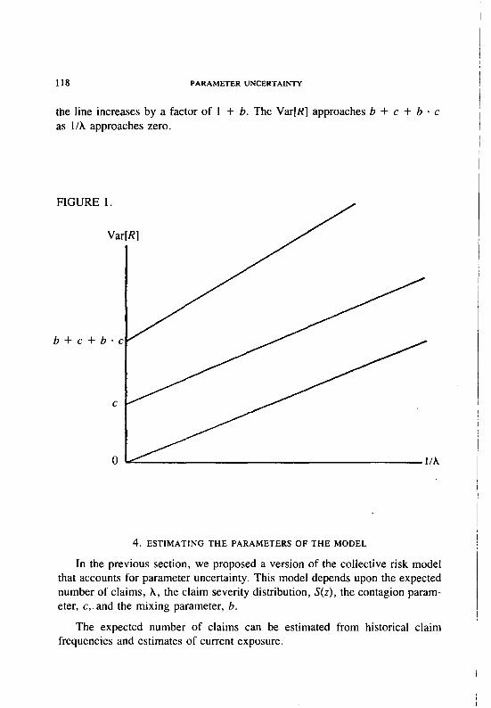
Figure 1 illustrates the effect of parameter uncertainty on Var[R]. If b = c = 0, the aggregate loss distribution is the generalized Poisson distribution. In this case Var[R] approaches zero as l/A approaches zero (or as the insured becomes larger). If we introduce parameter uncertainty in the claim count distribution, Var[R] lies on a line parallel to that implied by the generalized Poisson distribution, with the variance approaching c as l/A approaches zero. If we add parameter uncertainty in the claim severity distribution, the slope of
118 PARAMETER UNCERTAINTY
the line increases by a factor of 1 + b. The Var[K] approaches b + c + b - c as l/A approaches zero.
FIGURE 1.
Var[R]
b+c+b-c
lh
4. ESTIMATING THE PARAMETERS OF THE MODEL
In the previous section, we proposed a version of the collective risk model that accounts for parameter uncertainty. This model depends upon the expected number of claims, A, the claim severity distribution, S(z), the contagion param- eter, c, and the mixing parameter, b.
The expected number of claims can be estimated from historical claim frequencies and estimates of current exposure.
PARAMETER UNCERTAINTY 119
A complete discussion of estimating claim severity distributions is beyond the scope of this paper. In our work, we typically obtain claim severity distri- butions from bureau circulars, or we estimate them from company data using methods similar to those described by Patrik [8]. These claim severity distri- butions are often derived from experience other than that of.the insured under consideration. For this reason, we adjust the scale of the distribution to match the average claim size that we project for the insured.
Before discussing our methods for estimating b and c, we should mention the work of Patrik and John [9]. They deal with parameter uncertainty by picking a finite set of claim severity distributions and claim count distributions for the collective risk model. They then combine the various outputs of the model by taking a weighted average. The weights are probabilities which they assign subjectively.
The use of subjective probabilities has always been controversial. Many consider the word “guess” to be more appropriate. It is unfortunate that in many situations an answer is demanded, but no data is available. Under these circum- stances, the use of subjective probabilities may be acceptable.
Regardless of how one feels toward the use of subjective probabilities, one should always consider the possibility of estimating b and c from observations of aggregate loss data. The remainder of this section will develop ways of doing this.
We will describe two approaches for estimating b and c. The choice of estimators will depend on the kind of data available. The general idea underlying both of these approaches will be to evaluate an expression which “resembles” Var[Nl, Var[X] or Var[R]. Using Equations 3.2, 3.6 or 3.7, we can then set the expression equal to its expected value, which depends upon b and c. The estimates are then obtained by solving for b and c. The details are given in the appendices.
We first consider the case of a single insured for which we have r years of experience. We assume that all systematic adjustments of the data, such as trend and loss development, have been made.
The following estimators for b and c are derived in Appendix A.
Forj = l,..., r, let Nj be the claim count for yearj. Let ej be a number such that ej = K . E[Nj] for each year i. K is a constant of proportionality. The number ej represents either exposure or premium.
120 PARAMETER UNCERTAINTY
Let AI = (l/r) I: Nj * (eilej) and j=l
V = i((ellej) * Nj - Al)‘. j=l
Then an estimator for c is given by
V - (r - 1)/r i (f?Jej) . fii e=
j=l
(r-l)*fi: ’ (4.1)
Let x I ,. . . ,Xr be r independent aggregate loss amounts associated with N1 ,.. .,N,, respectively, and let Aj = Xj/Nj be average claim costs. Furthermore let
@ * i XjlN be an estimate of E[Zl, j=l
&’ be an estimate of Var[Zj, and
W = ,$, Nj * (Aj - b)‘.
Then an estimator for b is given by
6= W-(r- 1)-G’ (4.2)
(r - 1) . 5’ + 2 * (N - (l/N) i N$ j=l
We used Monte Carlo simulation to test the accuracy. of these estimators. Specifically, we selected a claim severity distribution (given in Exhibit I) along with c = 0.1 and b = 0.1 We then simulated aggregate losses and claim counts using Algorithm 3.3, and tested how well the estimates 6 and 2 compared with the selected b and c. We obtained 6’ by multiplying the coefficient of variation of our claim severity distribution by the estimate of E[Zj obtained from the simulation. The results of these tests are given in Table 1.
The averages and standard deviations of the estimates for r = 5, 25, 100, and 400 were based on 2000, 400, 100, and 25 trials, respectively. While the estimates of the errors are subject to simulation error, the above table suggests that one may need several hundred observations to accurately estimate b and c. Clearly, this is impossible for a single insured. We have repeated this experiment for different values of b and c and have gotten similar results.
Table 1 does not tell how much accuracy is necessary. To answer this, one must first ask how the collective risk model will be used. An almost certain use is the calculation of excess pure premium ratios. How much error one may tolerate for b and c will then depend on how much error one may tolerate for excess pure premium ratios.
Table 2 gives excess pure premium ratios for various sizes of insureds and various b's and c’s. The method of calculating the excess pure premium, ratios is that of Heckman and Meyers [2].
122
Entry Ratio
0.50 1.00 1.50 2.00 2.50
Entry Ratio
0.50 1.00 1.50 2.00 2.50
PARAMETER UNCERTAINTY
TABLE 2
EXCESS PURE PREMIUM RATIOS Expected Loss = l,OOO,OQO
Table 2 shows that significant differences in excess pure premium ratios result from different values of b and c. Taking this result along with the results indicated by Table 1, we are forced to the rather unpleasant conclusion that parameter uncertainty cannot be adequately quantified on the basis of the ex- perience of a single insured.
If we are to estimate b and c from empirical data, it would appear that our only alternative is to combine the experience of several insureds, and assume that the same b and c are appropriate for all of them. It is this question that we now address.
5. ESTIMATING THE PARAMETERS OF THE MODEL-ONTINUED
If we were to combine the experience of several insureds to estimate b and c, we might consider using the above estimators and treating the combined observations as annual observations of a single insured, We feel, however, that this would be inappropriate for the following reasons.
PARAMETER UNCERTAINTY 123
First, a key assumption in the estimation procedure for c is that the expected number of claims is directly proportional to the measurement of exposure. While this assumption may be appropriate for a single insured, different insureds may have different exposure bases or different inherent claim frequencies.
Second, a key assumption in the estimation procedure for b is that the same claim severity distribution is appropriate for all observations of a single insured. Different insureds can expect to have different claim severity distributions.
Below we will give estimators for b and c. The data requirements for these estimators are as follows.
For each insured and each year we require three items:
1. exposure, 2. incurred losses, and 3. incurred claim count.
Some remarks concerning the data requirements are in order.
First, it will be assumed that the exposure is directly proportional to the expected claim count for each insured. The constant of proportionality may vary with the insured. Many exposure bases, such as payroll, are inflation sensitive. Thus, trends in the exposure base that do not reflect expected claim count should
I be removed.
\ Second, it will be assumed that the expected claim severity is the same for
all observations of a\ single insured. The expected claim size need not be the same for all insureds. Incurred losses must be adjusted for trends in claim severity. The trend factors must be derived from external sources so as not to introduce bias in the estimates.
Third, every effort should be made to get the maximum number of obser- vations. A minimum of two observations per insured will be required. We should strive for the maximum number of observations per insured and the maximum number of insureds.
The following estimators for b and c are derived in Appendix A:
T = number of insureds ri = number of observations for insured i
,, Nii = number of claims for observation j of insured i eG = exposure for observation j of insured i Xij = incurred loss for observation j of insured i
124 PARAMETER UNCERTAINTK
Zi = a random variable denoting claim severity for insured i.
Note that Equations 5.1 and 5.2 reduce to Equations 4.1 and 4.2, respec- tively, when T = 1.
Many companies and rating bureaus do not have the data required for the
PARAMETER UNCERTAINTY 125
above estimators. However, all is not lost. We shall now show that it is possible to get rough estimates of b and c with quite a bit less data.
One of the predictions of this version of the collective risk model is the linear relationship of the squared coefficient of variation of the loss ratio with l/h (or equivalently, l/expected losses). See Equation 3.7 and Figure 1. The following estimators of b and c will exploit this relationship.
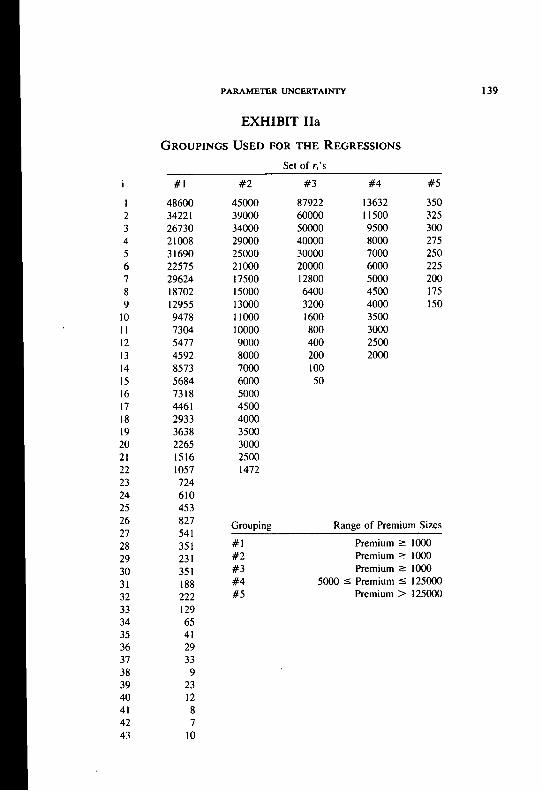
The data requirements for these estimators will be loss ratios and premiums for each insured, and a single claim severity distribution that represents all the insureds. Divide the insureds into T groups of size ri. For reasons stated above, we would prefer that the groups consist of multiple observations of the same insured. We shall say something about this in the next section. For observation j of group i, let
eij = exposure (premium), XV = incurred loss, and Rij = Xijley.
For each group i, let
ki = (llri) 5 Rij, j=l
Ei = (llri) 5 lieu, and j=l
Wf = ,$, (R, - @i)*.
An estimate of the squared coefficient of variation for the ith group is given by the expression
Wi
(Tim l)*tI:’
An estimate of l/expected losses for the ith group is given by the expression
Ei G’
Using linear regression, we can find an approximate relationship of the following form:
W ,. Ei . (ri - 1) . by = A * ; + B. (5.3)
126 PARAMETER UNCERTAINTY --
Estimators for b and c are then given by
6 = a . E[z]/E[Z*] - 1 and (5.4) c^ =(B - 6)/(1 + 6). (5.5)
These estimators for b and c are derived in Appendix B. As mentioned above, we must select a single claim severity distribution that represents all insureds. In practice, it is questionable that this can be done. If estimates are obtained in this manner, then the variance of the aggregate loss distribution will be overstated for the low severity insured and understated for the high severity insured. Meyers [4] discusses several problems associated with this. It should be noted that the linear relationship between the squared coefficient of variation and l/expected losses derived from Equation 5.3 will be preserved in the model if any reasonable claim severity distribution is selected. However, one should not put undue faith in the particular estimates of b and c.
6. TESTING THE MODEL
Thus far we have proposed a version of the collective risk model which allows for parameter uncertainty, and we have given ways to estimate the parameters for this model. We now turn to the crucial question, how well does
’ it fit empirical data?
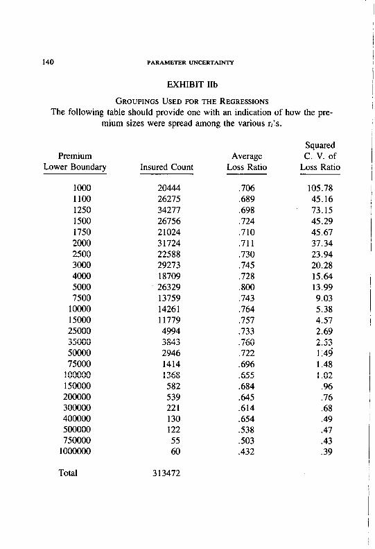
In 1980, a National Council committee assembled a large sample of indi- vidual insured data for the purpose of constructing a new table of excess pure premium ratios, otherwise known as Table M. This sample contained the stan- dard premium and the incurred losses for all insureds during the policy year beginning July 1, 1973 for all states in which the National Council had juris- diction.
The data was grouped by premium size, and the empirical loss ratio distri- butions were used to calculate the excess pure premium ratios for the smaller premium sizes. For those insureds with premium of $200,000 or more, it was felt that the empirical excess pure premiums were not credible, and so a combination of modeling and empirical data was used.,
After the table was completed, we requested and received from the National Council a tape containing this experience. This data forms the basis of our analysis.
PARAMETER UNCERTAlNn 127
Estimating the Parameters of the Model
Since we had only premium and loss data, we used Equations 5.4 and 5.5 with the eG’s representing standard premiums. Since we had only one observation for each insured, we chose our groups on the basis of premium size. Thus there are two main sources of parameter uncertainty. The first source is heterogeneity of insureds, and the second is differences in premium adequacy. This is consis- tent with the construction of the new Table M.
It should be noted that if we choose our groups on the basis of multiple observations on a single insured with the eu’s representing exposure, the sources of parameter uncertainty are quite different. Heterogeneity of insureds is not involved. Changes in the insured’s operations, changes in economic conditions, changes in loss development patterns and other changes over time are the main sources of parameter uncertainty. Thus, estimates of b and c under these con- ditions could be quite different.
At the time this study was done, the National Council did not have a claim severity distribution available. The closest thing we had to a comparable claim severity distribution was estimated from our own company data for accident year 1975 developed to 42 months. We chose 42 months because it matched the average maturity of the NCCI data. We then changed the scale of the distribution to match the average claim size which was reported by the National Council for the policy year 1973-74. The resulting claim severity distribution is given in Exhibit I.
In choosing the groups, we put those observations with the lowest r-1 pre- miums in the first group, those observations with the next lowest t-2 premiums in the second group, and so on. The problem remained of choosing the ri’s, i= 1,. . . , n for the n groups. We observed that when the ri’s were equal for all i the variance of the residuals of the regression decreased as the premium increased. In statistical terminology, this is known as heteroscedasticity. We dealt with this problem in two ways. One way was to have ri decrease as the premium increases. The other way was to use a weighted regression.
The weighted regression can be described as follows. If the model Y = AX + B + E is to be fitted, but if it appears that the standard deviation of E is proportional to X, then let Y’ = Y/X and let X’ = l/X. In the new model Y’ = A’ + B’X’ + E’, E’ will have approximately constant variance. A’ will be an estimate of A and B’ will be an estimate of B.
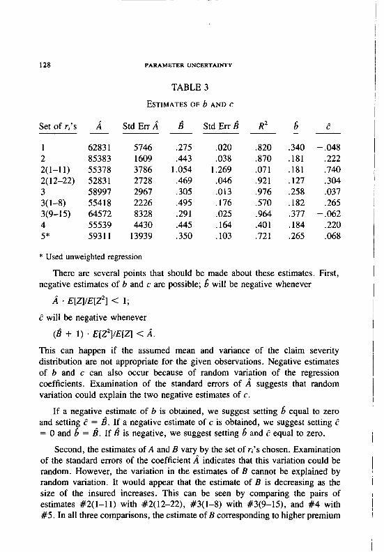
Exhibit II gives the various sets of ri’s that we considered. Table 3 gives the resulting estimates of b and c.
There are several points that should be made about these estimates. First, negative estimates of b and c are possible; 6 will be negative whenever
/i * E[z]/E[Z*] < 1;
E will be negative whenever
(b + 1) . E[Z*]/E[z] < A.
This can happen if the assumed mean and variance of the claim severity distribution are not appropriate for the given observations. Negative estimates of b and c can also occur because of random variation of the regression coefficients. Examination of the standard errors of A suggests that random variation could explain the two negative estimates of c.
If a negative estimate of b is obtained, we suggest setting 6 equal to zero and setting e = d. If a negative estimate of c is obtained, we suggest setting e = 0 and 6 = 8. If h is negative, we suggest setting 6 and e equal to zero.
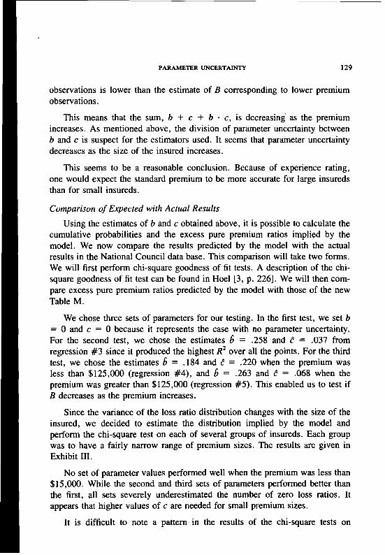
Second, the estimates of A and B vary by the set of ri’s chosen. Examination of the standard errors of the coefficient a indicates that this variation could be random. However, the variation in the estimates of B cannot be explained by random variation. It would appear that the estimate of B is decreasing as the size of the insured increases. This can be seen by comparing the pairs of estimates #2(1-11) with #2( 12-22), #3(1-8) with #3(9-15), and #4 with #5. In all three comparisons, the estimate of B corresponding to higher premium
PARAMETER UNCERTAINTY 129
observations is lower than the estimate of B corresponding to lower premium observations.
This means that the sum, b + c + b * c, is decreasing as the premium increases. As mentioned above, the division of parameter uncertainty between b and c is suspect for the estimators used. It seems that parameter uncertainty decreases as the size of the insured increases.
This seems to be a reasonable conclusion. Because of experience rating, one would expect the standard premium to be more accurate for large insureds than for small insureds.
Comparison of Expected with Actual Results
Using the estimates of b and c obtained above, it is possible to calculate the cumulative probabilities and the excess pure premium ratios implied by the model. We now compare the results predicted by the model with the actual results in the National Council data base. This comparison will take two forms. We will first perform chi-square goodness of fit tests. A description of the chi- square goodness of fit test can be found in Hoe1 [3, p. 2261. We will then com- pare excess pure premium ratios predicted by the model with those of the new Table M.
We chose three sets of parameters for our testing. In the first test, we set b = 0 and c = 0 because it represents the case with no parameter uncertainty. For the second test, we chose the estimates 6 = .258 and E = .037 from regression #3 since it produced the highest R* over all the points. For the third test, we chose the estimates 6 = .184 and L? = .220 when the premium was less than $125,000 (regression #4), and 6 = .263 and c? = .068 when the premium was greater than $125,000 (regression #5). This enabled us to test if B decreases as the premium increases.
Since the variance of the loss ratio distribution changes with the size of the insured, we decided to estimate the distribution implied by the model and perform the chi-square test on each of several groups of insureds. Each group was to have a fairly narrow range of premium sizes. The results are given in Exhibit III.
No set of parameter values performed well when the premium was less than $15,000. While the second and third sets of parameters performed better than the first, all sets severely underestimated the number of zero loss ratios. It appears that higher values of c are needed for small premium sizes.
It is difficult to note a pattern in the results of the chi-square tests on
130 PARAMETER UNCERTAMn
individual groups. The chi-square test is simply not powerful enough to distin- ugish between the various sets of parameter values on individual groups. How- ever, the chi-square test permits combining the results of independent tests. (Actually, the tests are not independent since the parameters b and c were estimated from all the observations. Since the number of observations used in estimating the parameters was far greater than .the number of observations in each chi-square test, however, the tests are very nearly independent.) When the results are combined, a clear pattern emerges.
The results predicted by the second and third sets of parameters are better than the results predicted by the parameters b = 0 and c = 0. Allowing for parameter uncertainty significantly improves the performance of the collective risk model. The results predicted by the third set of parameters are better than the results predicted by the second set for the smaller premium sizes. This is consistent with our hypothesis that B decreases as the size of the insured increases.
Comparisons with the new Table M are given in Exhibit IV. Again we see that allowing for parameter uncertainty significantly improves the performance of the collective risk model. While the model does not fit the new Table M perfectly, it does come reasonably close.
Interpretation of the Results
The combined chi-square statistic calculated in Exhibit III indicates that we should reject the hypothesis that aggregate losses have the distribution predicted by the model. This shows that we have indeed made a ‘number of simplifying assumptions.
This brings us back to the “Actuary’s Dilemma.” As noted above, the construction of an empirical Table M is suspect because of the necessity of using heterogeneous groups of insureds. It is extremely difficult to tell which is the more accurate. One must look to the applications in order to determine which to use.
Through the end of 1982, Table M was used to determine insurance charges in retrospective rating plans. The same insurance charges were used regardless of what claim severity distributions were appropriate for the insured and what accident limit was selected. Meyers [4] demonstrated that the claim severity distribution and the accident limit have a significant effect on the insurance charge. By examining Meyers’ tables, one can see that these differences are much larger than the differences between the collective risk model with param- eter uncertainty and the new Table M.
PARAMETER UNCERTAlNTY 131
A revision of the retrospective rating plan is currently being considered by the National Council. This revision contains an adjustment for the “overlap” between the insurance charge and the excess loss premium factor. This adjust- ment was derived using the collective risk model with parameter uncertainty.
While the “Actuary’s Dilemma” is not resolved, we see that the collective risk model with parameter uncertainty can make a significant contribution to the solution of today’s problems.
7. LARGE INSUREDS
As demonstrated above, it is necessary to combine the experience of several insureds to get stable estimates of b and c. The methods given for estimating b and c assume that these parameters are the same for all insureds. It seems unlikely that b and c are the same for all insureds. For example, a stable company that has been working in the same line of business for many years should have a lower b and c than a company that has recently made material changes to its operations. A detailed examination of a company’s operations may reveal additional sources of parameter uncertainty.
For small insureds, it may not be cost effective to conduct such an exami- nation. Thus, it should be acceptable to assume that b and c are the same for all small insureds.
For large insureds, close examinations are routine. It seems quite possible that an underwriter could more accurately quantify parameter uncertainty on the basis of judgmental factors. However, skeptical actuaries respond that while underwriters are very sensitive to both the natural desire to sell insurance and aversion to risk, their quantitative estimates depend very much on what the competition offers. We regard it as an open question as to which method performs the best.
What is an actuary to do under these circumstances? First, we should provide estimates of b and c based on the combined experience of several large insureds. As Morel1 [6] remarked in his review of the first version of this paper, “We owe them at least that much.” Furthermore, the data should contain several years of experience for each insured and the appropriate estimators for b and c should be used. Parameter uncertainty arising from heterogeneity between mem- bers of a group of insureds is not applicable for large account pricing.
If a close examination reveals additional sources of parameter uncertainty, sensitivity testing should be done to determine the effect of this uncertainty.
132 PARAMETER UNCERTAINTY
Quite often, the results of such testing can aid in designing a contract that is agreeable to all parties.
The remarks in this section are quite speculative. But they point out the need for extreme caution in using the collective risk model with large accounts.
8. CONCLUSION
This paper proposes a new version of the collective risk model that allows for uncertainty in selecting the expected number of claims and the claim severity distribution. We provide two different methods of estimating the parameters of this model. It is demonstrated by computer simulation that one must combine the experience of several insureds in order to accurately quantify parameter uncertainty. Tests on a very large sample of individual insured data show a significant improvement in the accuracy of the collective risk model when parameter uncertainty is taken into account. The tests do not show perfect agreement between the model and the empirical data, but the agreement is close enough to be useful in many applications.
9. ACKNOWLEDGEMENTS
We would like to thank the National Council for providing us with the data that was used in the paper. An earlier version of this paper was presented in the 1982 CAS call for papers. While preparing a teview, Roy Morel1 made several comments which aided us in preparing this version. We urge the reader to read his review [6]. We would like to thank Bradley Alpert, Yakov Avichai, Philip Heckman and Edward Seligman for their helpful comments.
PARAMETER UNCERTAINTY
APPENDIX A - DERIVATION OF EQUATIONS 4.1, 4.2, 5.1 AND 5.2
133
The equations derived in this appendix require the following data.
T = number of insureds ri = number of observations for insured i, (ri > 1)
Nij = number of claims for observation j of insured i eg = exposure for observation j of insured i Xij = incurred loss for observation j of insured i a: = an estimate of Var[Zi], where Zi is a random variable denoting claim
severity for insured i.
Estiniating c
Let Xii be the expected number of claims for insured i and observation j. Assume hij = Ki * eu. Then
It
Aij = Ail ’ c?fjlf?il.
follows from Equations 3.2 and A. 1 that
Var[Nij] = Xii . eij/eii + c * (hii * eo/eii)‘.
Let
(A.1)
(A.21
V= i .g (Nii ’ eilleij - &I)*. i=l j=l
Adding and subtracting Xii inside the parentheses gives us
v= g (5 (NV * eilleij - AU)* - ri * (ii, - Ail)’ . i=l j=l >
Equation 5.2 is obtained by substituting W for E[KINij’s], ii for pi and 6: for a:. Equation 4.2 is simply Equation 5.2 with T = 1.
APPENDIX B-DERIVATION OF EQUATIONS 5.4 AND 5.5
The equations derived in this appendix require that individual ObSeNatiOnS
be divided into T groups of size ri. They also require the first moment, E[Zl, and the second moment, E[Z*], of an assumed claim severity distribution.
For observation j of group i, let
eij = exposure (premium), Xii = incurred loss, and Ru =, Xijle~.
For each group i, let
pi = E[RQ], and
bi = (llri) 2 Rc. j=l
It follows from Equation 3.6 that
Var,R,,l = Pi * (1 Q 5) ’ E[Z*l V eii . E[Zj - + p’ . (b + c + b - c). (B.1)
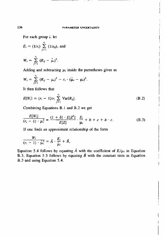
136
For each group i, let
Ei = (llri) 2 (lleij), j=l
Wi = 2 (Rg - bi)*. j=l
PARAMETER UNCERTAINTY
and
Adding and subtracting pi inside the parentheses gives us
Wi = ,$, (R, - ki)* - ri * (ki - pi)‘.
It then follows that
E[Wi] = (ri - l)lri i Var[Rij]. j=l
Combining Equations B. 1 and B.2 we get
EWil (ri - 1) * /.lJ =
(1 + b) * W*l . & + b + c + b . c EKI Pi
If one finds an approximate relationship of the form
Wi
03.2)
(B.3)
Equation 5.4 follows by equating a with the coefficient of Eilki in Equation B.3. Equation 5.5 follows by equating k with the constant term in Equation B.3 and using Equation 5.4.
r.11
PI
[31
[41
151
[61
171
PI
[91
[lOI
ill1
[=I
PARAMETER UNCERTAINTY
REFERENCES
137
R. E. Beard, T. Pentikainen, E. Pesonen (1977), Risk Theo& 2nd edition, Chapman and Hall.
P. Heckman and G. Meyers (1983), “The Calculation of Aggregate Loss Distributions from Claim Severity and Claim Count Distributions,” PCAS LXX.
P. G. Hoe1 (1971), Introduction to Mathematical Statistics, 4th edition, John Wiley and Sons.
G. Meyers (1980), “An Analysis of Retrospective Rating,” PCAS LXVII, p. 110.
G. Meyers, and N. Schenker (1982), “Parameter Uncertainty in the Col- lective Risk Model,” Pricing, Underwriting and Managing the Large Risk, Casualty Actuarial Society Discussion Paper Program, p. 253.
R. Morel1 (1982), “Discussion of Parameter Uncertainty in the Collective Risk Model,” Pricing, Underwriting and Managing the Large Risk, Cas- ualty Actuarial Society Discussion Paper Program, p. 300.
National Council on Compensation Insurance.
G. Patrik (1980), “Estimating Casualty Loss Amount Distributions,” PCAS LXVII, p. 57.
G. Patrik, and R. John (1980), “Pricing Excess-of-Loss Casualty Working Cover Reinsurance Treaties;” Pricing Property and Casualty Insurance Products, Casualty Actuarial Society Discussion Paper Program, p. 399.
L. J. Simon (1965), “The 1965 Table M,” PCAS LB; p. 1.
D. Skumick (1974), “The California Table L,” PCAS LXI, p. 117.
G. Venter (1982) “Transformed Beta and Gamma Distributions and Ag- gregate Loss,” Pricing, Underwriting and Managing the Large Risk, Cas- ualty Actuarial Society Discussion Paper Program, p. 395.