Khan, A., Razis, B., Gillespie, S., Percival, C., & Shallcross, D. (2017).Global analysis of carbon disulfide (CS2) using the 3-D chemistry transportmodel STOCHEM. AIMS Environmental Science, 4(3), 484-501. DOI:10.3934/environsci.2017.3.484

Publisher's PDF, also known as Version of record

License (if available):CC BY

Link to published version (if available):10.3934/environsci.2017.3.484

Link to publication record in Explore Bristol ResearchPDF-document

This is the final published version of the article (version of record). It first appeared online via AIMS Press athttp://www.aimspress.com/article/10.3934/environsci.2017.3.484/abstract.html. Please refer to any applicableterms of use of the publisher.

University of Bristol - Explore Bristol ResearchGeneral rights

This document is made available in accordance with publisher policies. Please cite only the publishedversion using the reference above. Full terms of use are available:http://www.bristol.ac.uk/pure/about/ebr-terms

AIMS Environmental Science, 4(3): 484-501.

DOI: 10.3934/environsci.2017.3.484

Received: 13 March 2017

Accepted: 17 May 2017

Published: 22 May 2017

http://www.aimspress.com/journal/environmental

Research article

Global analysis of carbon disulfide (CS2) using the 3-D chemistry

transport model STOCHEM

Anwar Khan1, Benjamin Razis

1, Simon Gillespie

1, Carl Percival

2,! and Dudley Shallcross

1,*

1 Atmospheric Chemistry Research Group, School of Chemistry, University of Bristol, Cantock’s

Close, Bristol BS8 1TS, UK 2

The Centre for Atmospheric Science, The School of Earth, Atmospheric and Environmental Science,

The University of Manchester, Simon Building, Brunswick Street, Manchester, M13 9PL, UK !

Now at NASA Jet Propulsion Laboratory, 4800 Oak Grove Dr, Pasadena, CA 91109, USA

* Correspondence: Email: d.e.shallcross@bristol.ac.uk; Tel: +44 (0) 117-928-7796.

Abstract: Carbon disulfide (CS2), a precursor to the long-lived carbonyl sulphide (OCS) is one of the main

contributors to the atmospheric sulfate layer. The annual fluxes from its sources and sinks are investigated

using a 3-D chemistry transport model, STOCHEM-CRI. In terms of the flux analysis, the oxidation of CS2

by OH is found to be the main removal process (76–88% of the total loss) and the dry deposition loss

contributes 11–24% to the total loss of CS2. The global burden of CS2 was calculated, varying between 6.1

to 19.2 Tg and the lifetime of CS2 was determined to be within the range of 2.8–3.4 days. The global

distribution of CS2 found the Northern Hemisphere (NH) continental landmasses to be the areas of

concentration maxima with peak concentrations reaching up to 20 ppt during June-July-August (J-J-A)

season and 40 ppt during December-January-February (D-J-F) season in anthropogenic source regions.

Oceanic regions returned low CS2 levels of less than 2 ppt. The vertical profile of CS2 shows higher

levels up to 3 ppt at 30°N–45°N during J-J-A and up to 4 ppt at 30°N–55°N during D-J-F. The oxidation

of CS2 by OH can produce a substantial amount (0.58 Tg/yr) of atmospheric OCS and the annual average

surface distribution of this flux shows up to 12 Tg/yr OCS formed in the regions with highest

anthropogenic pollution (e.g., South east Asia). In general, the model-measurement comparison reveals

an underprediction of model CS2 compared with measured CS2 for most of the regions. It is likely that

the emissions of CS2 are being underestimated and there are likely much larger emission sources of

atmospheric CS2 than previously suggested.

Keywords: Carbon disulfide; chemistry transport model; global budget; surface distribution;

zonal distribution

485

AIMS Environmental Science Volume 4, Issue 3, 484-501.

1. Introduction

Carbon disulfide (CS2) exerts a significant influence on the global atmospheric sulfur budget [1,2].

The principal source of CS2 is supposed to be oceanic [3-8], but spatial analysis of CS2 indicates large

concentrations over continental masses, suggesting the main sources of CS2 are of anthropogenic

origin [9-11]. Blake et al. [11] reported four major industrial sources of CS2 as black carbon

production, rayon manufacture, CS2 chemical production and use, and sulfur recovery. Ren [12] found

that carbonyl sulphide (OCS) converted to CS2 in the roots and shoots of barley and chickpeas,

suggesting it may be a precursor to CS2 in vegetation and soil. Soil has no consistent flux direction

for CS2 [13]. Soil and wetland fluxes of CS2 are sparse [10] because of the large variety of soil types

(e.g., oxic soils, anoxic soils) and wetland types (e.g., freshwater mangrove swamp, freshwater

grassy marsh, and paddy fields) which make them extremely hard to estimate.

The main removal process of CS2 is the photochemical oxidation with OH radicals producing

both sulfur dioxide (SO2) and OCS as the major products [14,15].

CS2 + OH OCS +SH (1a)

SH + O(3P) SO + H (1b)

SO + O2 SO2 + O (1c)

The oxidation of CS2 and the further oxidation of OCS form sulphate aerosols which can

influence the radiative properties of the Earth’s atmosphere, potentially contributing to climate

change and the stratospheric ozone concentration [9,16-20].

CS2 can also undergo removal by O(3P) radicals although this is negligible due to low O(

3P)

radical abundances in the troposphere [9].

CS2 + O(3P) CS + SO (2a)

CS2 + O(3P) OCS + S (2b)

CS + O(3P) CO + S (2c)

CS + O2 OCS + O (2d)

The photolysis of CS2 is possible only in the upper parts of the troposphere by shortwave

radiation, but very small at altitudes below 6 km [9].

CS2 + h CS + S (>280 nm) (3a)

CS + O2 OCS + O (3b)

S + O2 SO + O (3c)

SO + O2 SO2 + O (3d)

The dry deposition through vegetation can act as a significant loss process of CS2 [21], but this

is not consistent throughout the studies. Taylor et al. [22] reported CS2 deposition velocities in the

range of 0–1.5 mm/s. However, Xu et al. [21] reported CS2 deposition velocity of 5.6 mm s−1

with

large associated uncertainties at a spruce forest in the Solling Mountains, Germany. Wet deposition

loss is considered to be minimal due to CS2 being relatively insoluble [23].

The climatic significance of the atmospheric sulfur cycle is difficult to assess without accurate

estimation of the global atmospheric reduced sulfur compounds (e.g., OCS, DMS, and CS2). The

486

AIMS Environmental Science Volume 4, Issue 3, 484-501.

budget for DMS is relatively secure and balanced [10,24,25]; the budget of OCS was previously

considered balanced [10,26] but recent studies have shown large uncertainties in its global budget

with large missing sources [27-32]. There are very few modeling studies to estimate the global

budget and surface distribution of tropospheric CS2 [3,9,33-35], many uncertainties exist in the

assessments of its global budget [10]. In this study, we employ STOCHEM-CRI, a 3-D global

chemistry transport model, to evaluate the global budget and distribution of CS2 in the troposphere.

We show a comparison between model CS2 concentrations and a judicious selection of observed CS2

concentrations from individual field measurements and some flight data set.

2. Methodology

The global 3-D chemistry transport model, STOCHEM used in this study is from the UK

Meteorological Office. This model has been extensively evaluated and assessed in a number of

model inter-comparison exercises [36,37], which have shown it to be ideally suited to modeling

atmospheric chemistry at a level comparable with Eulerian models. The model uses a Lagrangian

approach, where the troposphere is divided into 50,000 air parcels which are advected every three

hours by winds from the UK Meteorological Office Hadley Centre general circulation model (GCM).

The Lagrangian cells are based on a grid of 1.25° longitude, 0.8333° latitude and 12 unevenly spaced

(with respect to altitude) vertical levels with an upper boundary of 100 hPa [38,39]. Each air parcel

contains the complete 231 trace gases in the code, which undergo chemical processes. The chemical

processes that occur within the parcel, together with emission, dry and wet deposition, mixing and

removal processes, are generally uncoupled from advection [39]. During the advection process, the

Lagrangian cells are considered to be isolated parcels of air and a treatment of mixing is achieved by

imposing a fixed Eulerian grid over the model domain [40]. At each timestep, trace species in

Lagrangian air parcels within a Eulerian grid cell are relaxed to the average of the trace species from

that group of parcels. Thus, the Eulerian mixing processes are artificially imposed on the Lagrangian

parcels to simulate the effects of diffusion in the atmosphere. Turbulent mixing in the boundary layer

is achieved by randomly re-assigning the vertical co-ordinates of air parcels over the depth of the

planetary boundary layer height. Small-scale convective processes are treated by randomly mixing a

fraction of the air parcels between the surface and the cloud top, depending on the convective cloud

top, convective cloud cover, and convective precipitation rate. Boundary layer and convection

parameterisations were fine-tuned by using 222

Rn observations [27]. Other meteorological variables,

such as cloud distributions, are kept fixed over the 3-hour chemistry model time-step [41]. More

detailed description of the meteorological parameterisations in STOCHEM can be found in Collins et

al. [38] with updates described by Derwent et al. [42].

The chemical mechanism used in STOCHEM, is the common representative intermediates

mechanism version 2 and reduction 5 (CRI v2-R5). The CRI v2-R5 was developed on a

compound-by-compound basis using 5-day box model simulations with the performance of the chemistry

for each compound being compared and optimised with the master chemical mechanism (MCM v3.1)

with ozone production being the primary criterion. The detail of the CRI v2-R5 mechanism is given by

Jenkin et al. [43], Watson et al. [44], and Utembe et al. [45] with updates highlighted in Utembe et al. [39]

and Utembe et al. [46]. In the study, the mechanism consists of 231 chemical species competing in 630

reactions and gives excellent agreement with the MCM v3.1 over a full range of NOx levels [43,44].

Emissions are treated as an additional term to the source fluxes of each species during each

integration time step, rather than a step change in species concentration [38,47]. Emission data for

487

AIMS Environmental Science Volume 4, Issue 3, 484-501.

oceans and soil is mapped onto a monthly, 5° longitude 5° latitude resolution, two-dimensional

source map [48]. The anthropogenic surface distribution of CS2 has been used as like SO2 surface

distribution which were based on EDGAR v3.2 data for 1995 [49]. Total emission values for CO,

NOx, and NMVOCs are obtained from the Precursor of Ozone and their Effects in the Troposphere

(POET) inventory [50] for the year 1998 with added emissions of CS2 from anthropogenic (0.34 Tg/yr),

soil + volcano (0.14 Tg/yr) and oceans (0.18 Tg/yr) taken from Watts [10]. Dry deposition is one of the

loss processes for CS2 which is accounted in the model via gravitational movement process.

Deposition velocity depends on the location of the air parcel and in the STOCHEM model, there is a

distinction made between air parcels over the sea and the land. The dry deposition velocities over

land and sea used in the model as 1.5 mm/s [22] and 0.1 mm/s (calculated from the gas transfer

velocity based on global average wind speed of ~8 m/s), respectively. The uptake of CS2 by

vegetation with the deposition velocity of 5.4 mm/s [21] was used as dry deposition over land with

unchanging deposition over sea (0.1 mm/s) in the model to investigate how the increment of dry

deposition over land can affect the global budget of tropospheric CS2. The photolysis rate of CS2 in

STOCHEM is calculated explicitly for each air parcel at a time resolution of one hour. The

photolysis rate of CS2 is calculated in STOCHEM using the following integral:

represents the photolysis rate constant of CS2;

represents the spherically integrated actinic flux at a given wavelength;

represents the cross section of CS2, at a given wavelength;

represents the quantum yield for dissociation of CS2 at a given wavelength.

The cross-section and quantum yields data were taken from Atkinson et al. [51]. More details

about the photolysis reactions implemented in STOCHEM can be found in Khan et al. [52].

The concentrations produced from the model simulation is mapped onto a Eulerian grid

resolution 5° 5° with 9 vertical levels. Summing the 50,000 air parcels produces a global burden

for CS2, which is broken down into the respective source and sink fluxes. The flux outputs are

calculated within each grid square by dividing the averaged emissions per air parcel (molecules s−1

)

by its volume, which gives volume-averaged fluxes with units of molecules cm−3

s−1

. Five

simulations, STOCHEM-base case detailed in Utembe et al. [39], STOCHEM-DEPO with increasing

deposition loss of CS2 over land, STOCHEM-PHOT with including photolysis loss of CS2,

STOCHEM-OCSL with increasing global oceanic and soil emissions of CS2 and STOCHEM-ANTH

with increasing global anthropogenic emissions of CS2 (Table 1) were conducted with meteorology

from 1998 for a period of 24 months with the first 12 allowing the model to spin up. Analysis is

performed on the subsequent 12 months of data.

The amount of measurement data from both surface stations and flight campaigns is very limited

and thus a judicious selection of data is used to evaluate the model simulations. The simulated data for

model-measurement comparison was extracted from the closest grid square to the region in question.

Some experimental data was taken for a large area and thus encompasses many grid boxes and in such

circumstances, data were extracted from multiple grid squares and the average was taken. The modeled

data are monthly averages for a given region adjusted to represent the months studied.

488

AIMS Environmental Science Volume 4, Issue 3, 484-501.

Table 1. Details of the simulations performed in the study.

Model simulation Loss processes Deposition velocity

(mm/s)

Emission class

STOCHEM-base CS2 + OH Products

k1 = 1.25 10−16exp(4550/T)/(1 + 1.81

10−13exp(3400/T)) cm3 molecules−1 s−1 [53]

CS2 + O(3P) Products

k2 = 3.2 10−11exp(−650/T) cm3 molecules−1 s−1

[53]

Land-1.5

Ocean-0.1

Anthropogenic-0.39 Tg/yr,

soil-0.09 Tg/yr,

ocean-0.18 Tg/yr [10]

STOCHEM-DEPO Same as base case Land-5.4 [21],

Ocean-0.1

Same as base case

STOCHEM-PHOT Same as base case and an additional reaction,

CS2 + h Products

Same as

STOCHEM-DEPO

Same as base case

STOCHEM-OCSL Same as STOCHEM-PHOT Same as

STOCHEM-DEPO

Anthropogenic-0.39 Tg/yr,

soil-0.9 Tg/yr,

ocean-0.7 Tg/yr [3]

STOCHEM-ANTH Same as STOCHEM-PHOT Same as

STOCHEM-DEPO

Anthropogenic-1.77 Tg/yr,

soil-0.17 Tg/yr,

ocean-0.58 Tg/yr [54]

3. Results and Discussion

3.1. Global budget of CS2

Table 2 details the production and loss processes of CS2. In this study, only the direct emissions

of CS2 from anthropogenic sources, oceans, soils had been integrated into the model. Three sinks of

CS2 were identified in the STOCHEM-base case: the reaction with OH, the reaction with O(3P) and

the dry deposition. Oxidation by OH radicals is found to be the main sink of CS2 (0.58 Tg/yr, 88% of

the total sinks), which is concordant with the data estimates (0.57 Tg/yr) from Chin and Davis [9]

and Watts [10] who estimated that oxidation by OH accounts for 56–100% of CS2 removal. The

simulated flux of the CS2 conversion to OCS contributes 43% of the total production flux of OCS

(1.31 Tg/yr) estimated by Watts [10]. The concentrations of O(3P) are very low across the

troposphere and hence the contribution of the loss process, CS2 + O(3P) is found to be very small

(<1%) in the study. The dry deposition is another sink of CS2 (0.07 Tg/yr, 11% of the total loss)

which has been found to be significant (0.15 Tg/yr, 23% to the total loss) after a 5-fold increment of

deposition velocity over land in the simulation, STOCHEM-DEPO. The emission fluxes of CS2 from

the previous four modeling studies [3,33-35] with a range of global emissions (0.4–2.4 Tg/yr) of CS2

used in their models (Table 2) gave a range of global burdens (7.8–80 Gg) and lifetimes (4–13 days).

However, in our model study, the global burden of CS2 is found to be small compared with the

studies of Pham et al. [33], Weisenstein et al. [34] and Khalil and Rasmussen [3], the discrepancy in

emission data is the likely reason for the disagreement between the results. The simulated lifetime of

CS2 for the STOCHEM-base is found to be 3.4 days, which is at the lower end of the range of

literature estimates shown in Table 2. The photolysis of CS2 has been ignored in all previous

modeling studies [35], but we included the photolysis of CS2 in STOCHEM-PHOT and found this

489

AIMS Environmental Science Volume 4, Issue 3, 484-501.

loss process very negligible (0.01 Gg/yr) compared with other loss processes. The inclusion of emission

classes of Khalil and Rasmussen [3] in STOCHEM-OCSL (increased global soil and oceanic emissions

in the model) and Lee and Brimblecombe [54] in STOCHEM-ANTH (increased global anthropogenic

emissions in the model) increases the global burden of CS2 to 16.2 Gg and 19.2 Gg, respectively which

are 212 and 271% increments relative to the STOCHEM-PHOT. Thus, when emissions are the only

atmospheric source of a compound, a range of emission classes makes it difficult to ensure an accurate

and valid output from a modeling study. The oxidation of CS2 by OH in STOCHEM-OCSL and

STOCHEM-ANTH can provide a substantial amount of atmospheric OCS, 1.6 Tg/yr and 1.9 Tg/yr,

respectively.

Table 2. The global budget of CS2. The values (except global burden and lifetime)

given are masses of CS2 in Tg/yr for the total production and loss. The percentage

contributions of the loss processes are shown in parenthesis.

STOCH

EM-base

STOCHE

M-DEPO

STOCHE

M-PHOT

STOCHE

M-OCSL

STOCHEM

-ANTH

Pham et al.

[33]

Kjellström

[35]

Weisenstein

et al. [34]

Khalil and

Rasmussen [3]

Production

Direct emission 0.66 0.66 0.66 1.99 2.52 1.19 0.43 2.38 2.0

Removal

OH oxidation 0.578

(88.4)

0.504

(77.0)

0.504

(77.0)

1.583

(80.5)

1.890

(75.7)

1.19 0.43 2.35 0.6

Reaction with O(3P) 0.002

(0.3)

0.001

(0.2)

0.001

(0.2)

0.004

(0.2)

0.005

(0.2)

n/a n/a n/a n/a

Dry deposition 0.074

(11.3)

0.149

(22.8)

0.149

(22.8)

0.379

(19.3)

0.602

(24.1)

n/a n/a n/a 0.1

Photolysis n/a n/a 0.00001

(0.0)

0.00001

(0.0)

0.00004

(0.0)

n/a n/a n/a 0

Other 1.3

Global Burden (Gg) 6.11 5.18 5.19 16.17 19.23 11.8 7.8 45.1 70.0

Lifetime (days) 3.4 2.9 3.0 3.0 2.8 4.0 6.5 7.0 13.0

Notes: *n/a represents no available data.

3.2. Global surface distribution of CS2

The surface distributions of CS2 in STOCHEM-base (Figure 1) show a difference between the

continental regions in the northern hemisphere (NH) and southern hemisphere (SH) with increased

CS2 concentrations of up to 20 pptv during June-July-August (J-J-A) and up to 40 pptv during

December-January-February (D-J-F) over anthropogenic emission regions (e.g., North America,

central Europe and South East Asia) in the NH. The surface distribution pattern of CS2 in our model

is comparable with the studies of Pham et al. [33] and Kjellström et al. [35] who also found highest

concentrations of CS2 over areas of industrial activity. However, the magnitude of surface CS2 levels

in our study is found to be more variable than their studies which are most likely due to the different

emission classes used in the models as well as because of the different resolutions of the models. For

example, the emissions total used in STOCHEM (this study) is slightly higher than that used in

490

AIMS Environmental Science Volume 4, Issue 3, 484-501.

IMAGES by Pham et al. [33], but 2-fold lower than that used in ECHAM3 by Kjellström et al. [35]

(see Table 2), but the vertical resolution of STOCHEM (9 vertical levels) is coarser than that of

IMAGES (25 vertical levels) and ECHAM3 (19 vertical levels). The surface layer is taken between

the surface and 1 km in STOCHEM compared with the models IMAGES and ECHAM3 which were

taken from 30–35 m and therefore much greater dilution by mixing and removal that can take place

in STOCHEM. Thus, the decreased vertical resolution of STOCHEM may give rise to the lower

mixing ratios of CS2 from areas of increased anthropogenic emissions.

The east coast of the US and South East Asia reach elevated concentrations of up to 20 pptv

during J-J-A (Figure 1A) which reflects the increased industrial activities of these areas. Europe has

background CS2 concentrations of between 3–7 ppt with several hot spots of high CS2 concentrations

reaching up to 15 ppt over Eurasia (e.g., Turkey) and the Middle East (e.g., Iraq, Saudi Arabia)

(Figure 1A) most likely attributed to the oil, gas, and petrochemical industries as well as increased

anthropogenic pollution. There are a few hot spots of CS2 (e.g., 10 ppt) in the southern continental

regions such as South Africa (Figure 1A). The elevated CS2 concentrations around South Africa are

expected because of its significant petrochemical, plastic, and synthetic fibre industries [55]. In

South America, there appear to be two areas (e.g., near Rio de Janeiro and Northern Brazil) of

increased CS2 concentrations (2–3 ppt) are most likely to be due to increased anthropogenic

emissions partly due to the high population densities in these places.

(A) (B)

Figure 1. The average surface level distribution of CS2 simulated by the

STOCHEM-base for (A) J-J-A and (B) D-J-F seasons.

During D-J-F, there is a significant increment in concentrations over the continental landmasses (e.g.,

up to 40 ppt in south East Asia, Figure 1B). This is to be expected as removal by OH accounts for 88% of

CS2 removal and in D-J-F months, OH concentrations in the NH are far lower than that of the J-J-A

months. The global oceanic emissions of CS2 (0.18 Tg/yr) integrated in the STOCHEM-base model

resulted in the concentrations of CS2 between 1 to 3 ppt in most of the oceanic regions. This indicates that

3 ppt is the annual average upper limit of CS2 concentrations from open ocean. In a variety of open ocean

areas regions exist with concentrations of less than 1 ppt.

The inclusions of increased soil and oceanic emissions in STOCHEM-OCSL and increased

anthropogenic emissions in STOCHEM-ANTH increase the concentration of CS2 relative to the

491

AIMS Environmental Science Volume 4, Issue 3, 484-501.

STOCHEM-PHOT by up to 800% (Figure 2A) in the regions of Amazon rainforest, central and

southern Africa and Australia and by up to 400% in the regions of North America, central Europe and

South East Asia (Figure 2B), respectively. These increased amounts of CS2 can enhance the oxidation

products (e.g., OCS, SO2) which can alter the formation of the global atmospheric sulfate layer.

(A) (B)

Figure 2. The percentage change of surface CS2 level (A) from STOCHEM-PHOT

to STOCHEM-OCSL and (B) from STOCHEM-PHOT to STOCHEM-ANTH.

CS2 is the most important precursor gas to OCS, for which a large missing source is needed to

balance sources and sinks [28-32]. The flux analysis using the STOCHEM-base model shows that up

to 12 Tg OCS /yr per grid box can be formed from the reaction CS2 + OH in the regions (Figure 3A)

with very high anthropogenic pollution (e.g., South east Asia). Incorporating the global

anthropogenic emissions of CS2 [54] in the STOCHEM-ANTH model produces up to 40 Tg OCS /yr

per grid box in South East Asia (Figure 3B). This revised production of OCS from CS2 can play an

especially important role over South East Asia regions, where comparisons between measurements

and anthropogenic emission inventories show a significant missing source of OCS [11].

3.3. Global vertical distribution of CS2

The vertical profile data in STOCHEM-base (Figure 4) shows the decay of CS2 concentrations

as altitude increases. The J-J-A season vertical distribution shows higher levels of CS2 up to 3 ppt at

30°N–45°N (Figure 4A) due to the larger surface concentrations over the latitude due to areas of high

anthropogenic emissions from Europe and North America. A very small area (0–15°S) of higher CS2

(1.5 ppt) is visible in the tropics (Figure 4A) because of the increased oceanic emissions. Heading

south from 30°S latitude to 90°S, CS2 is found in small amounts throughout the troposphere. In

general, the model OH concentration decreases from the equator for each altitude bin, and so the loss

of CS2 via reaction with OH decreases in a similar way (Figure 4A). During D-J-F, the CS2

concentration is also found to be higher (up to 4 ppt) in the region of 30–55oN (Figure 4B) due to the

larger anthropogenic activity, but the vertical distribution of CS2 for D-J-F mirrors that of J-J-A;

lower OH concentration in the NH during D-J-F leads to lower removal of CS2 and therefore it can

reach higher altitudes in the region of 60–90oN. During D-J-F, the peak in the tropics disappears due

492

AIMS Environmental Science Volume 4, Issue 3, 484-501.

to the decreased emissions from ocean but another peak at the region of 50–60oS appears due to the

increased emissions from SH oceans.

(A) (B)

Figure 3. The annual average surface distribution of OCS production from the

oxidation of CS2 simulated by (A) the STOCHEM-base (B) the STOCHEM-ANTH.

(A) (B)

Figure 4. The average zonal distribution of CS2 simulated by the STOCHEM-base

for (A) J-J-A and (B) D-J-F seasons.

The vertical CS2 distribution shows similarities to the vertical profile found by Kjellström [35].

Both profiles display peaks around 60oN and 60

oS, but the concentrations seen in this study are

found to be smaller than that in Kjellström [35]. Ultimately, as the emission data and the resolution

of the two studies are different, it is unsurprising that the absolute concentrations are different, yet

what is encouraging is that despite these factors, the annual vertical distributions are similar.

493

AIMS Environmental Science Volume 4, Issue 3, 484-501.

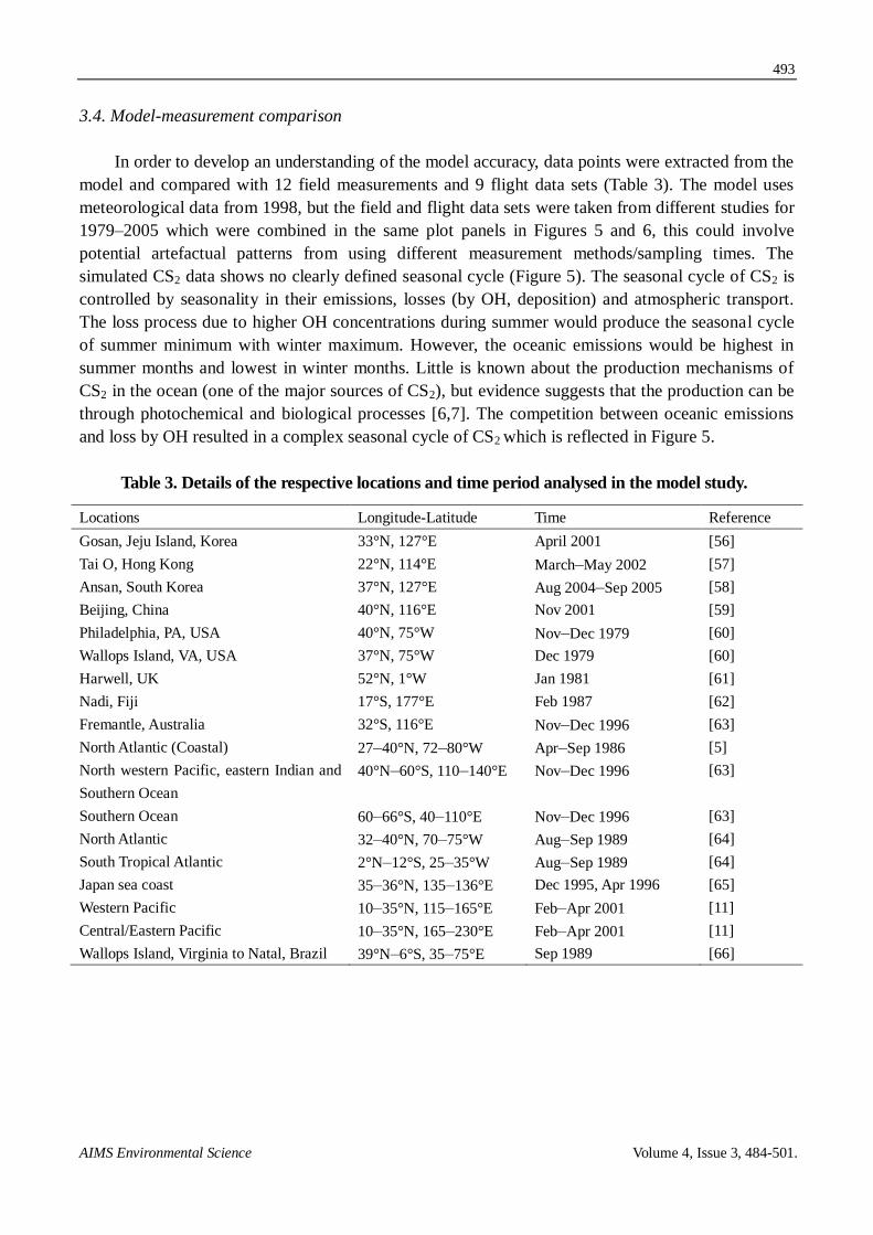
3.4. Model-measurement comparison

In order to develop an understanding of the model accuracy, data points were extracted from the

model and compared with 12 field measurements and 9 flight data sets (Table 3). The model uses

meteorological data from 1998, but the field and flight data sets were taken from different studies for

1979–2005 which were combined in the same plot panels in Figures 5 and 6, this could involve

potential artefactual patterns from using different measurement methods/sampling times. The

simulated CS2 data shows no clearly defined seasonal cycle (Figure 5). The seasonal cycle of CS2 is

controlled by seasonality in their emissions, losses (by OH, deposition) and atmospheric transport.

The loss process due to higher OH concentrations during summer would produce the seasonal cycle

of summer minimum with winter maximum. However, the oceanic emissions would be highest in

summer months and lowest in winter months. Little is known about the production mechanisms of

CS2 in the ocean (one of the major sources of CS2), but evidence suggests that the production can be

through photochemical and biological processes [6,7]. The competition between oceanic emissions

and loss by OH resulted in a complex seasonal cycle of CS2 which is reflected in Figure 5.

Table 3. Details of the respective locations and time period analysed in the model study.

Locations Longitude-Latitude Time Reference

Gosan, Jeju Island, Korea 33°N, 127°E April 2001 [56]

Tai O, Hong Kong 22°N, 114°E March–May 2002 [57]

Ansan, South Korea 37°N, 127°E Aug 2004–Sep 2005 [58]

Beijing, China 40°N, 116°E Nov 2001 [59]

Philadelphia, PA, USA 40°N, 75°W Nov–Dec 1979 [60]

Wallops Island, VA, USA 37°N, 75°W Dec 1979 [60]

Harwell, UK 52°N, 1°W Jan 1981 [61]

Nadi, Fiji 17°S, 177°E Feb 1987 [62]

Fremantle, Australia 32°S, 116°E Nov–Dec 1996 [63]

North Atlantic (Coastal) 27–40°N, 72–80°W Apr–Sep 1986 [5]

North western Pacific, eastern Indian and

Southern Ocean

40°N–60°S, 110–140°E Nov–Dec 1996 [63]

Southern Ocean 60–66°S, 40–110°E Nov–Dec 1996 [63]

North Atlantic 32–40°N, 70–75°W Aug–Sep 1989 [64]

South Tropical Atlantic 2°N–12°S, 25–35°W Aug–Sep 1989 [64]

Japan sea coast 35–36°N, 135–136°E Dec 1995, Apr 1996 [65]

Western Pacific 10–35°N, 115–165°E Feb–Apr 2001 [11]

Central/Eastern Pacific 10–35°N, 165–230°E Feb–Apr 2001 [11]

Wallops Island, Virginia to Natal, Brazil 39°N–6°S, 35–75°E Sep 1989 [66]

494

AIMS Environmental Science Volume 4, Issue 3, 484-501.

Figure 5. Monthly variation of the surface CS2 abundances of selected monitoring

stations produced by the STOCHEM-CRI. Blue, green, red and bottle green lines

represent mean calculated values of CS2 produced by the STOCHEM-base, the

STOCHEM-DEPO, the STOCHEM-OCSL, and the STOCHEM-ANTH,

respectively. Black triangle symbols represent the measurement data of CS2 and the

error bars represent measurement variability.

The area best modeled is the marine boundary layer likely due to this area being subject to

insignificant amounts of anthropogenic emissions, but an underprediction with a mean bias of −2.7 ppt

for the modeled data compared with the measured data is found when looking at regions within marine

clean environments (e.g., North Atlantic, Southern Ocean, Pacific, eastern Indian and Southern Ocean).

The global oceanic emissions of CS2 are highly variable ranging from 3.3 to 2346 Gg/yr for different

marine environments [8], but we used the global oceanic emissions of 180 Gg/yr in the STOCHEM-base

case which can explain the discrepancies between model and measured CS2 in the marine environment.

Increasing the global soil and oceanic emissions [3] in the STOCHEM-OCSL brings the model into

closer agreement (mean bias reduces to −0.6 ppt) with measurements for these marine campaigns. The

oceanic emissions of CS2 are unclear because of lacking process understanding, a further

investigation into how the discrepancies can be improved would be highly desirable.

The correlation between modeled and measured CS2 is found to be very good for some clean

areas (e.g., Jeju Island in Korea, Fremantle in Australia), but the CS2 concentrations in approximately

background air (relatively unpolluted air) arriving at the east coast of the USA, Philadelphia and

Wallops Island and in air arriving at rural areas Harwell, UK and Tai O, Hong Kong are reported as

36 pptv in November, 40 pptv in December, 15 pptv in January and 47 pptv in March-April-May,

respectively [56,59,60] which equates to a large underprediction (mean bias of −24.7 ppt) of the

simulated values by STOCHEM-base (Figure 6). Harwell and Tai O are located in the rural

environment, but there are nearby industrialized areas which may contain large anthropogenic

sources of CS2 which can be advected into the rural areas increasing the ambient rural conditions.

495

AIMS Environmental Science Volume 4, Issue 3, 484-501.

Increasing the global anthropogenic emissions of CS2 in the STOCHEM-ANTH model improves the

agreement with measurements (the mean bias reduces to −1.0 ppt) for these locations. Relatively low

concentrations of simulated CS2 are found in Fiji which are likely to be due to the absence of

significant anthropogenic sources surrounding the area. The measured data collected near Fiji

recorded concentrations as high as 12 pptv, because there are significant biomass burning events in

the area [62], which may have skewed the results and therefore may be unrepresentative of Fiji’s

natural ambient condition. Due to limited data within the remote SH and hence clean atmospheric

conditions, this hypothesis couldn’t be tested any further. Increased experimental data within the

remote SH would help to validate global atmospheric models and perhaps filling this void should be

a focus of future expeditions.

Air samples collected from industrial areas (e.g., Beijing, China and Ansan, South Korea) found

very high concentrations of CS2 due to the anthropogenic emissions, giving very large

underprediction of the STOCHEM-ANTH modeled values with a mean bias of −490 ppt compared

with the measured values. Due to the large difference in magnitude it is likely that there may be

additional sources of CS2 currently being under-estimated or not being accounted for, suggesting

primarily that anthropogenic emissions are likely to be much larger than current estimates. In

addition, the coarse resolution of STOCHEM model (5° latitude 5° longitude) makes it difficult to

accurately model CS2 in highly polluted areas which make up only a small fraction of the grid. The

meteorological data incorporated in STOCHEM was from the year 1998 which was one of the

strongest El Niño years in the past 50 years, this could lead to differences in the model data when

compared with measured data from other years. Consideration of inter-annual variation give better

representation of the model data which could improve the disagreement between model and

measured data.

Figure 6 shows the vertical distributions of CS2 over the North Atlantic, South tropical Atlantic,

Western Pacific, Central/Eastern Pacific, Wallops Island-Virginia to Natal-Brazil, and Japan sea coast

with the simulated data overlaid. The modeled CS2 at different altitude levels for North Atlantic and

South tropical Atlantic fit within one standard deviation of the measured mean except one outlier at

3.5 km. The STOCHEM-base case simulation underpredicted CS2 by on average 1.5 ppt in North

Atlantic and South tropical Atlantic and increasing the global ocean and soil emissions in the model,

STOCHEM-OCSL reduces the underprediction by 47%. In the North Atlantic, the concentration at

the surface is almost four times higher than that found in the South Atlantic because of the possible

higher anthropogenic emissions of CS2 in NH than that in SH. The global distribution of CS2 (Figure 1)

indicates that Europe and the east coast of the US have much higher concentrations compared with

South America and Africa and thus through mixing and advection might have influenced CS2

concentrations above the ocean [64]. In addition, the area of the South Atlantic that was sampled in

this study was closer to the equator, thus higher OH concentrations yielding increased CS2 removal

and lower atmospheric concentrations.

In extremely polluted environments e.g., the Japan sea-coast (part of the NASA Transport and

Chemical Evolution over the Pacific (TRACE-P) campaign to investigate outflow from polluted

Asian regions and clean air from the Pacific Ocean), STOCHEM-base underpredicted the CS2

concentrations in the Japan sea-coast with a mean bias of −64 ppt suggesting that the emissions of

CS2 integrated in the model are likely to be underestimated. The long-range transport of CS2 from

the source regions on the Asian continental outflow mixing with marine air over the Japan Sea can be

responsible for the higher CS2 over Japan sea coast [63]. The coarse model resolution (5° 5°) of

496

AIMS Environmental Science Volume 4, Issue 3, 484-501.

STOCHEM is responsible for model underprediction over the Japan sea-coast because it cannot

represent typical Asian continental pollution with sufficient spatial accuracy. Increasing the global

anthropogenic emissions of CS2 in the STOCHEM-ANTH model reduces the model-measurement

mean bias to −55 ppt. There are some other marine flight campaigns as part of TRACE-P e.g.,

Western Pacific and Central/Eastern Pacific, where the mean bias for STOCHEM-base is found to be

−3.2 ppt. STOCHEM-OCSL and STOCHEM-ANTH simulations reduces the mean biases to 22%

and 53%, respectively. In the study, a more comprehensive regional comparison with the literature

was intended but there is a lack of up-to-date measurement data, more field and flight measurement

data would be invaluable to validate our model accuracy.

Figure 6. Vertical profiles for measured and modeled CS2. Blue, green, red, and

bottle green lines represent mean calculated values of CS2 produced by the

STOCHEM-base, STOCHEM-DEPO, STOCHEM-OCSL, and STOCHEM-ANTH,

respectively. Black triangles represent the measurement CS2 data and the black

error bars represent measurement variability.

4. Conclusion

The global analysis for CS2 was performed using a 3-D chemistry and transport model,

STOCHEM-CRI which was concordant with several literature sources suggesting that the model

results show a tendency towards underestimation. A suit of simulation results give the global burden

and lifetime of CS2 as 6.1 to 19.2 Tg and 2.8–3.4 days, respectively. The global surface distribution

of CS2 displayed the expected characteristics; with highest concentrations over areas of industrial

activities. Comparing the global surface and vertical distribution of CS2 simulated by the

STOCHEM-CRI with other model studies suggested that the trends are found to be in good

497

AIMS Environmental Science Volume 4, Issue 3, 484-501.

agreement with the concentrations simulated by IMAGES and ECHAM3. The oxidation of CS2

produces a large amount (0.5–1.9 Tg/yr) of OCS which can reduce the imbalance between the

sources and the sinks of OCS. Increasing oceanic emissions in the model reduces the

model-measurement disagreement significantly for the marine campaigns. The major

underprediction by the model in polluted areas is likely due to the level of anthropogenic emissions

being much greater than previously thought but also due to the coarse resolution of STOCHEM.

Currently many of the campaigns have looked at very similar areas, for example the Global

Tropospheric Experiment/Chemical Instrumentation Test and Evaluation (GTE/CITE 3) and Global

Atmospheric Measurements Experiment of Tropospheric Aerosols and Gases (GAMETAG)

expeditions have carried out extensive sampling around the East coast of USA, the Atlantic Ocean

and down to South America. The TRACE-P study looked in detail at China, South East Asia, Korea

and Japan, yet there has been very little sampling from Europe, the Middle East and the SH in

general. Such experimental data will be the key to validate our model results.

Acknowledgements

We thank NERC and Bristol ChemLabS under whose auspices various aspects of this work

were carried out.

Conflict of interest

We declare that there is no conflict of interest in this paper.

References

1. Wine PH, Chameides WL, Ravishankara AR (1981) Potential role of CS2 photooxidation in

tropospheric sulfur chemistry. Geophys Res Lett 8: 543-546.

2. Andreae MO (1990) Ocean-atmosphere interactions in the global biogeochemical sulfur cycle.

Mar Chem 30: 1-29.

3. Khalil MAK, Rasmussen RA (1984) Global sources, lifetimes and mass balances of carbonyl

sulphide (OCS) and carbon disulfide (CS2) in the Earth’s atmosphere. Atmos Environ 18:

1805-1813.

4. Leck C, Rodhe H (1991) Emissions of marine biogenic sulfur to the atmosphere of northern

Europe. J Atmos Chem 12: 63-86.

5. Kim K-H, Andreae MO (1992) Carbon disulfide in the estuarine, coastal, and oceanic

environments. Marine Chem 40: 179-197.

6. Xie H, Moore RM, Miller WL (1998) Photochemical production of carbon disulphide in

seawater. J Geophys Res 103: 5635-5644.

7. Xie H, Moore RM, Miller WL (1999) Carbon disulfide in the North Atlantic and Pacific oceans.

J Geophys Res 104: 5393-5402.

8. Kettle AJ, Rhee TS, von Hobe M, et al. (2001) Assessing the flux of different volatile sulfur

gases from the ocean to the atmosphere. J Geophys Res 106: 12193-12209.

9. Chin M, Davis DD (1993) Global sources and sinks of OCS and CS2 and their distributions.

Global Biogeochem. Cycles 7: 321-337.

498

AIMS Environmental Science Volume 4, Issue 3, 484-501.

10. Watts SF (2000) The mass budgets of carbonyl sufide, dimethyl sulphide, carbon disulfide and

hydrogen sulphide. Atmos Environ 34: 761-779.

11. Blake NJ, Streets DG, Woo JH, et al. (2004) Carbonyl sulphide and carbon disulfide: large-scale

distributions over the western Pacific and emissions from Asia during TRACE-P. J Geophys Res

109: D15.

12. Ren YL (1999) Is carbonyl sulfide a precursor for carbon disulfide in vegetation and soil?

Interconversion of carbonyl sulfide and carbon disulfide in fresh grain tissues in vitro. J Agric

Food Chem 47: 2141-2144.

13. Steinbacher M, Bingemer HG, Schmidt U (2004) Measurements of the exchange of carbonyl

sulfide (OCS) and carbon disulfide (CS2) between soil and atmosphere in a spruce forest in

central Germany. Atmos Environ 38: 6043-6052.

14. Stickel RE, Chin M, Daykin EP, et al. (1993). Mechanistic studies of the OH-initiated oxidation

of CS2 in the presence of O2. J Phys Chem 97: 13653-13661.

15. Seinfeld JH, Pandis SN (2006) Atmospheric Chemistry and Physics: From Air Pollution to

Climate Change, 2 Eds., John Wiley and Sons, Inc., New Jersey: 1-1203.

16. Crutzen PJ (1976) The possible importance of CSO for the sulfate layer of the stratosphere.

Geophys Res Lett 3: 73-76.

17. Hofmann DJ (1990) Increase in the stratospheric background sulfuric acid aerosol mass in the

past 10 years. Science 248: 996-1000.

18. Taubman SJ, Kasting JF (1995). Carbonyl sufide: No remedy for global warming. Geophys Res

Lett 22: 803-805.

19. Chin M, Davis DD (1995) A reanalysis of carbonyl sulphide as a source of stratospheric

background sulfur aerosol. J Geophys Res Atmos 100: 8993-9005.

20. Bruhl C, Lelieveld J, Tost H, et al. (2015). Stratospheric sulfur and its implications for radiative

forcing simulated by the chemistry climate model EMAC. J Geophys Res-Atmos 120:

2103-2118.

21. Xu X, Bingemer HG, Schmidt U (2002) The flux of carbonyl sulphide and carbon disulfide

between the atmosphere and a spruce forest. Atmos Chem Phys 2: 171-181.

22. Taylor Jr GE, McLaughlin Jr SB, Shriner DS, et al. (1983). The flux sulfur-containing gases to

vegetation. Atmos Environ 17: 789-796.

23. De Bruyn WL, Swartz E, Hu JH, et al. (1995) Henry’s law solubilities and setchenow

coefficients for biogenic reduced sulfur species obtained from gas-liquid uptake measurements.

J Geophys Res 100: 7245-7251.

24. Berglen TF, Berntsen TK, Isaksen SA, et al. (2004) A global model of the coupled

sulphur/oxidant chemistry in the troposphere: The sulphur cycle. J Geophys Res 109: D19310.

25. Kloster S, Feichter J, Maier-Reimer E, et al. (2006) DMS cycle in the marine ocean-atmosphere

system- a global model study. Biogeosciences 3: 29-51.

26. Kettle AJ, Kuhn U, Von Hobe M, et al. (2002) Global budget of atmospheric carbonyl sulfide:

Temporal and spatial variations of the dominant sources and sinks. J Geophys Res 107: D22.

27. Suntharalingam P, Kettle AJ, Monzka SM, et al. (2008) Global 3-D model analysis of the

seasonal cycle of atmospheric carbonyl sulfide: Implications for terrestrial vegetation uptake.

Geophys Res Lett 35: L19801.

28. Berry J, Wolf A, Campbell JE, et al. (2013) A coupled model of the global cycles of carbonyl sulfide

and CO2: A possible new window on the carbon cycle. J Geophys Res-Biogeo 118: 842-852.

499

AIMS Environmental Science Volume 4, Issue 3, 484-501.

29. Kuai L, Worden JR, Campbell JE, et al. (2015) Estimate of carbonyl sulfide tropical oceanic

surface fluxes using Aura Tropospheric Emission Spectrometer observations. J Geophys

Res-Atmos 120: 11012-11023.

30. Glatthor N, Höpfner M, Baker IT, et al. (2015) Tropical sources and sinks of carbonyl sulfide

observed from space. Geophys Res Lett 42: 10082-10090.

31. Kremser S, Thomason LW, von Hobe M, et al. (2016) Stratospheric aerosol-Observations,

processes, and impact on climate. Rev Geophys 54: 278-335.

32. Lennartz ST, Marandino CA, von Hobe M, et al. (2017) Direct oceanic emissions unlikely to

account for the missing source of atmospheric carbonyl sulfide. Atmos Chem Phys 17: 385-402.

33. Pham M, Müller J-F, Brasseur GP, et al. (1995) A three-dimensional study of the tropospheric

sulfur cycle. J Geophys Res 100: 26061-26092.

34. Weisenstein DK, Yue GK, Ko MKW, et al. (1997) A two-dimensional model of sulfur species

and aerosols. J Geophys Res 102: 13019-13035.

35. Kjellström E (1998) A three-dimensional global model study of carbonyl sulphide in the

troposphere and the lower stratosphere. J Atmos Chem 29: 151-177.

36. Stevenson DS, Collins WJ, Johnson CE, et al. (1998) Intercomparison and evaluation of

atmospheric transport in a Lagrangian model (STOCHEM), and an Eulerian model (UM), using 222

Rn as a short-lived tracer. Quat J Royal Meteorol Soc 124: 2477-3492.

37. Stevenson DS, Dentener FJ, Schultz MG, et al. (2006) Multimodel ensemble simulations of

present-day and near-future tropospheric ozone. J Geophys Res 111: D08301.

38. Collins WJ, Stevenson DS, Johnson CE, et al. (1997) Tropospheric ozone in a Global-Scale

Three-Dimensional Lagrangian Model and its response to NOx emission controls. J Atmos Chem

26: 223-274.

39. Utembe SR, Cooke MC, Archibald AT, et al. (2010) Using a reduced Common Representative

Intermediates (CRI v2-R5) mechanism to simulate tropospheric ozone in a 3-D Lagrangian

chemistry transport model. Atmos Environ 13: 1609-1622.

40. Derwent RG, Collins WJ, Jenkin ME, et al. (2003) The global distribution of secondary

particulate matter in a 3-D Lagrangian chemistry transport model. J Atmos Chem 44: 57-95.

41. Stevenson DS, Johnson CE, Highwood EJ, et al. (2003) Atmospheric impact of the 1783–1784

Laki eruption: Part I chemistry modelling. Atmos Chem Phys 3: 487-507.

42. Derwent RG, Stevenson DS, Doherty RM, et al. (2008) How is surface ozone in Europe linked

to Asian and North American NOx emissions? Atmos Environ 42: 7412-7422.

43. Jenkin ME, Watson LA, Utembe SR, et al. (2008) A Common Representative Intermediate (CRI)

mechanism for VOC degradation. Part-1: gas phase mechanism development. Atmos Environ 42:

7185-7195.

44. Watson LA, Shallcross DE, Utembe SR, et al. (2008) A Common Representative Intermediate

(CRI) mechanism for VOC degradation. Part 2: gas phase mechanism reduction. Atmos Environ

42: 7196-7204.

45. Utembe SR, Watson LA, Shallcross DE, et al. (2009) A Common Representative Intermediates

(CRI) mechanism for VOC degradation. Part 3: Development of a secondary organic aerosol

module. Atmos Environ 43: 1982-1990.

46. Utembe SR, Cooke MC, Archibald AT, et al. (2011) Simulating secondary organic aerosol in a

3-D Lagrangian chemistry transport model using the reduced Common Representative

Intermediates mechansim (CRI v2-R5). Atmos Environ 45: 1604-1614.

500

AIMS Environmental Science Volume 4, Issue 3, 484-501.

47. Collins WJ, Stevenson DS, Johnson CE, et al. (2000) The European regional ozone distribution

and its links with the global scale for the years 1992 and 2015. Atmos Environ 34: 255-267.

48. Olivier JG, Bouwman AF, Berdowski JJ, et al. (1996) Description of EDGAR Version 2.0: A set

of global emission inventories of greenhouse gases and ozone-depleting substances for all

anthropogenic and most natural sources on a per country basis and on 1 degree 1 degree grid.

Technical report, Netherlands Environmental Assessment Agency.

49. Olivier JGJ, Berdowski JJM (2001) Global emissions sources and sinks. Berdowski JJM,

Guicherit R, Heij BJ (Eds.). The Climate System, Swets and Zeitlinger Publishers, Lisse,

Netherlands.

50. Granier C, Lamarque JF, Mieville A, et al. (2005) POET, a database of surface emissions of

ozone precursors. Available from: http://accent.aero.jussieu.fr/database_table_inventories.php.

51. Atkinson R, Baulch DL, Cox RA, et al. (2004) Evaluated kinetic and photochemical data for

atmospheric chemistry: Volume I-gas phase reactions of Ox, HOx, NOx and SOx species. Atmos

Chem Phys 4: 1461-1738.

52. Khan MAH, Cooke MC, Utembe SR, et al. (2015) A study of global atmospheric budget and

distribution of acetone using global atmospheric model STOCHEM-CRI. Atmos Environ 112:

269-277.

53. Sander SP, Friedl RR, Golden DM, et al. (2006) Chemical kinetics and photochemical data for

use in atmospheric studies. Evaluation number 15, JPL publication 06-2, Jet Propulsion

Laboratory, Pasadena, CA.

54. Lee CL, Brimblecombe P (2016) Anthropogenic contributions to global carbonyl sulfide, carbon

disulfide and organosulfides fluxes. Earth-Sci Rev 160: 1-18.

55. Majozi T, Veldhuizen P (2015) The chemicals industry in South Africa. American Inst. Chem.

Eng (AlChE) July: 46-51. Available from:

https://www.aiche.org/sites/default/files/cep/20150746.pdf

56. Kim KH, Swan H, Shon ZH, et al. (2004) Monitoring of reduced sulfur compounds in the

atmosphere of Gosan, Jeju Island during the Spring of 2001. Chemosphere 54: 515-526.

57. Guo H, Simpson IJ, Ding AJ, et al. (2010) Carbonyl sulphide, dimethyl sulphide and carbon

disulfide in the Pearl River Delta of southern China: Impact of anthropogenic and biogenic

sources. Atmos Environ 44: 3805-3813.

58. Pal R, Kim KH, Jeon EC, et al. (2009) Reduced sulfur compounds in ambient air surrounding an

industrial region in Korea. Environ Monit Assess 148: 109-125.

59. Yujing M, Hai W, Zhang X, et al. (2002) Impact of anthropogenic sources on carbonyl sulphide

in Beijing City. J Geophys Res 107: D24.

60. Maroulis PJ, Bandy AR (1980) Measurements of atmospheric concentrations of CS2 in the

eastern United States. Geophys Res Letts 7: 681-684.

61. Jones BMR, Cox RA, Penkett SA (1983) Atmospheric chemistry of carbon disulphide. J Atmos

Chem 1: 65-86.

62. Thornton DC, Bandy AR (1993). Sulfur dioxide and dimethyl sulfide in the central pacific

troposphere. J Atmos Chem 17: 1-13.

63. Inomata Y, Hayashi M, Osada K, et al. (2006) Spatial distributions of volatile sulfur compounds

in surface seawater and overlying atmosphere in the northwestern Pacific Ocean, eastern Indian

Ocean, and Southern Ocean. Global Biogeochem Cycles 20: GB2022.

64. Cooper DJ, Saltzman ES (1993) Measurements of atmospheric dimethylsulphide, hydrogen

501

AIMS Environmental Science Volume 4, Issue 3, 484-501.

sulphide, and carbon disulfide during GTE/CITE 3. J Geophys Res 98: 23397-23409.

65. Inomata Y, Iwasaka Y, Osada K, et al. (2006) Vertical distributions of particles and sulfur gases

(volatile sulfur compounds and SO2) over East Asia: comparison with two aircraft-borne

measurements under the Asian continental outflow in spring and winter. Atmos Environ 40:

430-444.

66. Bandy AR, Thornton DC, Johnson JE (1993) Carbon disulfide measurements in the atmosphere

of the western north Atlantic and the northwestern south Atlantic oceans. J Geophys Res-Atmos

98: 23449-23457.

© 2017 Dudley E. Shallcross et al., licensee AIMS Press. This is

an open access article distributed under the terms of the Creative

Commons Attribution License

(http://creativecommons.org/licenses/by/4.0)