Global and multiscale aspects of magnetospheric dynamics...

Global and multiscale aspects of magnetospheric dynamics in

local-linear filters

A. Y. Ukhorskiy, M. I. Sitnov, A. S. Sharma, and K. PapadopoulosDepartment of Physics, University of Maryland at College Park, College Park, Maryland, USA

Received 6 November 2001; revised 23 May 2002; accepted 10 July 2002; published 16 November 2002.

[1] The magnetospheric dynamics consists of global and multiscale components. Thelocal-linear filters (LLFs) relating the solar wind input and the magnetospheric output havebeen used earlier to predict the global dynamical behavior. In this paper, the relative role ofglobal and multiscale processes in the prediction of magnetospheric dynamics is studied.The filters are derived from the reconstructed input–output magnetospheric phase spaceusing time series of VBS as the input and AL index as the output. We show that theconventional formula for the LLF can be broken into two parts corresponding to the globaland multiscale constituents. The first part is the zeroth-order term, which is obtained by thephase space average of the model outputs. This is a feature similar to the mean-field modelin phase transition physics, which yields iterative predictions of the global coherentcomponent. The second part consists of the higher-order terms of the filter, which arehighly irregular and thus cannot be used in dynamical prediction. This irregular behaviorrepresents the departure from the low-dimensional dynamics underlying earlier studiesusing LLFs. The earlier prediction studies mixed these two components. However, byseparating these two components, the prediction procedure is highly simplified and longerperiod predictions are achieved. The multiscale nature arises from the perturbations over awide range of scales and has a power spectrum similar to that of colored noise. Whenthese perturbations are taken into account in the prediction process, the iterativepredictions yield a factor of four improvement in the accuracy compared to the mean-fieldmodel. However, the filter technique does not provide a prescription for correctlyincluding the multiscale aspects in a dynamical model and further improvement inforecasting can be achieved by a statistical approach. These results have importantimplications for space weather forecasting. INDEX TERMS: 2139 Interplanetary Physics:

Interplanetary shocks; 2164 Interplanetary Physics: Solar wind plasma; 2102 Interplanetary Physics:

Corotating streams; 2111 Interplanetary Physics: Ejecta, driver gases, and magnetic clouds; 7513 Solar

Physics, Astrophysics, and Astronomy: Coronal mass ejections; KEYWORDS: magnetosphere, substorm,

chaos, filters, phase transitions, SOC

Citation: Ukhorskiy, A. Y., M. I. Sitnov, A. S. Sharma, and K. Papadopoulos, Global and multiscale aspects of magnetospheric

dynamics in local-linear filters, J. Geophys. Res., 107(A11), 1369, doi:10.1029/2001JA009160, 2002.

1. Introduction

[2] The solar wind energy penetrates into the magneto-sphere by magnetic field line reconnection at the daysidemagnetopause, giving rise to magnetospheric substorms.Due to the imbalance between the reconnection rate onthe dayside magnetopause and at the distant neutral line afraction of the solar wind energy is accumulated in themagnetotail, mainly in the form of magnetic energy, and isthen suddenly released. Substorms have a variety of distinctmanifestations in the ionosphere (magnetic field perturba-tions at the polar regions, auroral brightening, particleprecipitation) as well as in the mid and distant magnetotail(plasmoid formation and ejection). Magnetospheric activity

during substorms extends from small-scale processes, suchas pseudobreakups, MHD turbulence, and current disrup-tion, to large-scale processes, such as global convection,field line depolarization, and plasmoid ejection. Thus, themagnetosphere behaves as a nonlinear, open, spatiallyextended system, which on the one hand is well organizedon global scale and on the other hand exhibits activity overa wide range of spatial and temporal scales.[3] There has been a considerable progress in the model-

ing and understanding the solar wind–magnetosphere cou-pling using nonlinear dynamical techniques. In this approachthe system evolution is described directly from data, usingspecial techniques such as time delay embedding, singularspectrum analyses, linear and local-linear filters (LLFs)[Sharma et al., 1993; Sharma, 1995; Vassiliadis et al.,1995]. The clear advantage of data-derived models is theirability to reveal inherent features of dynamics even in the

JOURNAL OF GEOPHYSICAL RESEARCH, VOL. 107, NO. A11, 1369, doi:10.1029/2001JA009160, 2002

Copyright 2002 by the American Geophysical Union.0148-0227/02/2001JA009160$09.00

SMP 15 - 1

presence of complexity and strong nonlinearity. The earlierdynamical models of the magnetospheric activity weremotivated by the global coherence indicated by the geo-magnetic indices and inspired by the concept of dynamicalchaos. They were based on the assumption that the observedcomplexity of the system is mainly attributed to the non-linear dynamics of a few dominant degrees of freedom[Sharma, 1995; Klimas et al., 1996]. Studies of the magneto-sphere as a dynamical system using modern techniques ofdata processing and phase space reconstruction [Grass-berger and Procaccia, 1983; Abarbanel et al., 1993] basedon AE index time series gave evidences of low effectivedimension of the magnetosphere [Vassiliadis et al., 1990;Sharma et al., 1993]. Further elaboration of this hypothesisresulted in creating space weather forecasting tools based onLLF with autoregression [Price et al., 1994; Vassiliadis etal., 1995; Sharma, 1995] and data-derived analogues [Kli-mas et al., 1992]. The low-dimensional organized behaviorof the magnetosphere during substorms is also evident inmany spacecraft in situ observations including the INTER-BALL and GEOTAIL missions [Ieda et al., 1998; Nagai etal., 1998; Petrukovich et al., 1998]. These studies confirmsuch key features of the globally coherent dynamics asplasmoid ejection, field line dipolarization, generation ofhot earthward plasma flows, etc.[4] However subsequent studies have shown that not all

aspects of magnetospheric dynamics during substorms con-form to the hypothesis of low dimensionality and thuscannot be accounted within the framework of dynamicalchaos and self-organization. For example, the power spec-trum of AE index data [Tsurutani et al., 1990] and magneticfield fluctuations in the tail current sheet [Ohtani et al.,1995] have a power law form typical for high-dimensionalcolored noise. Prichard and Price [1992] have argued thatusing a modified correlation integral [Theiler, 1991] a lowcorrelation dimension cannot be found for the magneto-spheric dynamics. Moreover, detailed analyses [Takalo etal., 1993, 1994] have shown that the qualitative propertiesof the AE time series are much more similar to bicolorednoise than to the time series generated by low-dimensionalchaotic systems. One interpretation of these multiscaleaspects of magnetospheric dynamics was suggested to bea multifractal behavior generated by intermittent turbulence[Consolini et al., 1996; Borovsky et al., 1997; Chang, 1998;Angelopoulos et al., 1999]. Another popular approach tomagnetosphere modeling is based on the concept of self-organized criticality (SOC) [Bak et al., 1987]. SOC explic-itly takes into account the large number of degrees offreedom and the interactions among them on differentscales. According to SOC models [Consolini, 1997; Chap-man et al., 1998; Uritsky and Pudovkin, 1998; Chang,1999; Takalo et al., 1999; Watkins et al., 1999; Klimas etal., 2000] multiscale behavior arises spontaneously andrequires no tuning of the system parameters, in other wordsSOC is attractor of dynamics.[5] Although SOC can account for the characteristic

power spectra observed in a number of processes duringsubstorms it is doubtful that SOC alone can provide theframework for modeling the solar wind–magnetospherecoupling. Indeed, it turns out that SOC, which was devel-oped to model sand pile behavior, is oversimplified even formodeling real sand piles [Nagel, 1992]. Violations of SOC

behavior were detected in observations of particle injectionsin the near-Earth magnetosphere [Borovsky et al., 1993;Prichard et al., 1996] and substorm chorus events [Smithet al., 1996]. Besides, the magnetosphere is essentiallynonautonomous with dynamics governed to a large extentby the external driver, the solar wind, while in SOC thecriticality is reached by a fine tuning of the control parameter(i.e., driving rate) to the vanishing value [Vespignani andZapperi, 1998]. Some models that internally exhibit SOCcan simultaneously generate non-SOC global instabilities[Chapman et al., 1998]. However, since such system-wideavalanches were found only in the simplified sand pilemodels, this still cannot account for the specific coherentfeatures of the actual magnetospheric dynamics. Moreover,since the fluctuations of the system at a critical point arecompletely uncorrelated it removes the possibility of evenshort-term predictability of the system’s evolution while itwas clearly demonstrated [Sharma, 1995; Vassiliadis et al.,1995; Valdivia et al., 1996] that input–output models yieldgood predictions of global magnetospheric activity.[6] One of the ways to reconcile global and multiscale

aspects of dynamics in unified model is suggested by thephysics of phase transitions. There are two different types ofphase transitions, which are intimately related to each otherand naturally coexist in a single system. The first-order phasetransitions are characterized by a low-dimensional manifoldin the phase space, e.g., the temperature–pressure–densitysurface for water-steam transitions. In first-order phasetransitions the first derivative of the state parameter of thesystem like density in water-steam transition or magnet-ization in ferromagnets is discontinuous. The distinctivefeature of second-order phase transitions, which representthe behavior of the system at criticality (i.e., in the vicinity ofthe singular point of the phase transition surface), is theirscale invariance reflected by various power law spectra andcritical exponents [Stanley, 1971]. Phase transitions in realnonautonomous systems are essentially dynamic and arenonequilibrium which results in additional properties likehysteresis and dynamical critical exponents [Hohenberg andHalperin, 1977; Chakrabarti and Acharyya, 1999; Zheng etal., 1999]. It has been noted [Sitnov et al., 2000, 2001;Sharma et al., 2001] that the magnetospheric dynamicsduring substorms shares a number of properties with non-equilibrium phase transitions. In particular, it was shown thatmultiscale substorm activity resembles second-order phasetransitions, while the large-scale perturbations reveal thefeatures of first-order nonequilibrium transitions includinghysteresis and global structure similar to the ‘‘temperature–pressure–density’’ diagram. Although the phase transitionanalogy gives an insight into various properties of themagnetospheric dynamics its implications to the forecastingof magnetospheric evolution are not clear yet.[7] The main purpose of the paper is to study the role of

multiscale processes in the prediction of magnetosphericdynamics. The multiscale processes have been ignored inthe earlier studies and this has limited the quality of thepredictions. The LLFs relating the solar wind input and themagnetospheric output are used to analyze the relative rolesof global and multiscale constituents of the magnetosphericbehavior during substorms.[8] It is found that in spite of the low dimensionality

assumption that lies underneath the LLF model, filters are

SMP 15 - 2 UKHORSKIY ET AL.: MAGNETOSPHERIC DYNAMICS IN LOCAL-LINEAR FILTERS

still capable of mimicking the multiscale high-dimensionalcomponent of magnetospheric dynamics. We show that theconventional formula for LLF can be broken into two parts,which are responsible for different dynamical constituents.The first part, the zeroth-order term of LLF, is the phasespace average of the model outputs, which is similar to themean-field model in phase transitions. It yields iterativepredictions of AL dynamics naturally separating the globalcoherent component from the time series. We also showthat the second part, which consists of the higher-orderterms of the filter, is irregular and thus is irrelevant forpredictions. This irregular behavior indicates the fundamen-tal difference between low-dimensional scale-invariantdynamic systems like Lorenz attractor and the magneto-sphere, which does not possess low dimensionality onsmaller scales. Nevertheless, the higher-order terms in thefilter formula still can model multiscale constituents of themagnetospheric dynamics, whose properties, both statisticaland dynamical are very similar to those of systems atcriticality.[9] The next section describes the LLFs and how they

represent the global and multiscale features of the solarwind–magnetosphere system. In section 4 the predictionsof the global magnetospheric dynamics using the centerof mass component of LLF is discussed. The multiscaleaspects modeled in section 5 by data reconstruction, andthis yields an estimate of the complexity in terms of thedimensionality of the space needed to represent thesystem. The last section presents the main results ofthe paper and their implications to space weather fore-casting.

2. Time Delay Embedding, Center of Mass, andLLFs

[10] In this section we discuss the primary aspects ofconstructing a dynamical model of nonautonomous (input–output) system based on LLFs with autoregression [Abar-banel et al., 1993; Sauer, 1993; Vassiliadis et al., 1995]. Inthis model a scalar time series I(t) is used as the input whichyields the output of the model O(t).[11] It is assumed that the scalar time series data of

observable quantities is a function only of the state of theunderlying system and contains all the information neces-sary to determine its evolution. Thus, if a space largeenough to unfold the dynamical attractor is reconstructedfrom the time series and the present state of the system isidentified, then the information about the future can beinferred form the known evolution of similar states.[12] For nonlinear dynamical models the phase space of

the system is reconstructed first using the time delayembedding method [Packard et al., 1980; Takens, 1981;Broomhead and King, 1986; Sauer et al., 1991]. Theembedding theorem [Takens, 1981] states that in theabsence of noise, if M � 2N + 1, then M-dimensionaldelay vectors generically form an embedding of the under-lying phase space of the N-dimensional dynamical system.Although Takens theorem is strictly valid for autonomoussystems only, numerous studies [e.g., Casdagli, 1992;Sharma, 1995; Vassiliadis et al., 1995; Sitnov et al.,2000] have used successfully the delay embedding methodfor modeling nonautonomous dynamical systems. In this

case the M-dimensional embedding space is formed byinput–output delay vectors:

~xn ¼ ~In; ~On

� �T

¼ In; In�1; . . . ; In� Mi�1ð Þ;On;On�1; . . . ;On� Mi�1ð Þ� �T ð1Þ

where In = I(t0 + n � t), On = O(t0 + n � t), t is the delaytime, Mi + Mo = M. If the delay matrix A is defined as:

A ¼~xT0...

~xTNt

0B@

1CA ð2Þ

C ¼ ATA ¼XNk¼0

~xk �~xk; C~vk ¼ w2k~vk;~vk 2 RM; k ¼ 1; :;M

ð3Þ

then C is the covariance matrix. Since C is hermitian bydefinition, its eigenvectors ~vkf g form an orthonormal basisin the embedding space. ~vkf g are usually calculated by usingthe singular value decomposition (SVD) method, accordingto which any M � N matrix A can be decomposed as:

A ¼ U �W � VT ¼XMk¼1

wk �~uk �~vk ð4Þ

where

V ¼ ~v1; . . . ;~vMð Þ;U ¼ ~u1; . . . ;~uMð Þ;W ¼ diagðw1; . . . ;wMÞ; U � UT ¼ 1;V � VT ¼ 1

On the other hand when the effective dimension of thesystem is not known, it is not clear beforehand what numberM of delays will provide embedding of the underling phasespace. Broomhead and King [1986] noted using the Lorenzsystem that the singular spectrum {wk} of the delay matrixdecreases until it reaches a plateau due to the noise in thesystem. They suggested that M should be the point were thesignal turns into noise. However, it turns out that real opensystems do not always behave this way. In particular, usingVBS–AL time series Sitnov et al. [2000] have shown that inthe case of magnetosphere the singular spectrum has welldefined power spectral shape that is retained over a widerange of scales with no clear sign of a distinctive noise floor.Hence, it is not always possible to find the appropriate valueof M using SVD only. In this work we demonstrate thatLLFs themselves can be used for determining the embeddingspace dimension when applied in an inverse problemmanner. That is, if M is considered as a free parameter ofthe model, then the prediction error can be minimized withrespect to this parameter, and the M value which provides theminimum error gives the embedding space dimension.[13] If the embedding procedure was properly performed,

that is, if the attractor of the system was completelyunfolded, then the projection of delay vectors on the basisconstructed with SVD yields the reconstructed states of thesystem. These reconstructed states have one-to-one corre-spondence with the states in the original phase space andthus can be used for predictions of the future evolution of

UKHORSKIY ET AL.: MAGNETOSPHERIC DYNAMICS IN LOCAL-LINEAR FILTERS SMP 15 - 3

the system [Farmer and Sidorowich, 1987; Casdagli, 1989,1992; Sauer, 1993]. For this purpose it is assumed that theunderlying dynamics can be described as a nonlinear scalarmap Onþ1 ¼ Fð~In; ~OnÞ, which relates the current state tothe manifestation of the following state, the output timeseries value at the next time step. The unknown nonlinearfunction F is approximated locally for each step of the mapby the linear filter:

Onþ1 F0 þ d~In; d ~On

� �T

� ~a~b

�

¼ F ~ICn ;~OC

n

� �þ

XMi�1

i¼0

ai In�i � ICn;i

� �þ

XMo�1

j¼0

bj On�j �OCn;j

� �ð5Þ

where ð~I C

n ; ~OC

n ÞTis the point about which the expansion is

made. The parameters of the filter (ai, bj, and F0) arecalculated using the known data, which is referred to as thetraining set. The training set is searched for the states similarto the current, that is the states that are closest to it, asmeasured by the distance in the embedding space definedusing the Euclidean metric. These states are referred to asnearest neighbors. LLFs in the form of (5) are also known aslocal-linear ARMA filters [Detman and Vassiliadis, 1997],since the linear term on the right hand side of (5) iscomposed of a moving average (MA) part, i.e., the weightedaverage of preceding inputs, and an autoregressive (AR)part, i.e., the sum of previous outputs.[14] The zeroth-order term in (5) is a function of the center

of expansion, the choice of which is, strictly speaking,ambiguous and should be justified in each particular case.For AE and Dst time series forecasting Price et al. [1994]and Valdivia et al. [1996] have used the expansion about theorigin. Another possible center of expansion can be thereference point, ð~In; ~OnÞT. For chaotic time series forecast-ing in autonomous dynamical systems Sauer [1993] sug-gested that better predictability is achieved when the averagestate vector of NN nearest neighbors is taken as the center ofexpansion:

~In; ~On

� �T� �

NN

¼ 1

NN

XNNk¼1

~Ikn;~Ok

n

� �T

ð6Þ

which is also called the center of mass, since (6) is theformula for the center of mass of NN identical particles withcoordinates ð~I kn ; ~O

k

nÞ. In this case, if the whole expression(5) is averaged over NN nearest neighbors, the leading termin the expansion F0 becomes hOn+1iNN, i.e., the arithmeticaverage of the outputs corresponding to one step iteratednearest neighbors. The resulting expression for the LLFstakes the form:

Onþ1 ¼ Onþ1h iNNþXMi�1

i¼0

ai In�i � ~In� �

NN

� �

þXMo�1

j¼0

bj On�j � ~On

D ENN

� �ð7Þ

Vassiliadis et al. [1995] used local-linear ARMA filters withexpansion around the center of mass for both the short andlong-term predictions of auroral indices, which gave better

results than the model of Price et al. [1994]. It may seemthat choosing the center of mass as the expansion center forthe filter function is an auxiliary procedure that leads tosome increase in the prediction accuracy. However, as wewill show later in the paper, in the case of Earth’smagnetosphere, and presumably for a large class ofnonautonomous real systems, expansion about the centerof mass may be the essential element of modeling thesystem’s dynamics with the use of LLFs. It allows aseparation of the regular component of the dynamics,stabilizes the prediction algorithm, and provides the basisfor modeling the multiscale portion of the dynamics.Moreover, we demonstrate that, as was earlier noted byKennel and Isabell [1992] for the case of autonomoussystems, if the filter function is expanded about the center ofmass, the linear terms in equation (7) are irrelevant and canbe omitted, as far as long-term predictions are concerned;the best prediction results can be achieved using only thezero-order terms.[15] When the center of mass is calculated, equation (7) is

applied to each of the nearest neighbors. This results in NNlinear equations with M unknowns, viz. filter coefficientsai, bj and can be expressed as:

ANN~y ¼~b ð8Þ

~y ¼ ~a~b

� ;~b ¼

O1nþ1 � Onþ1h iNN

..

.

ONNnþ1 � Onþ1h iNN

0B@

1CA;

ANN ¼

~I1n;~O1

n

� �T

� ~In; ~On

� �T� �

NN

..

.

~INNn ; ~ONNn

� �T

� ~In; ~On

� �T� �

NN

0BBBBB@

1CCCCCA

This system of equation is solved in the least squares sensewith use of SVD:

~y ¼ A�1NN~b ¼

XM0

k¼1

1

wNNk

~b �~uNNk� �

~vNNk ð9Þ

where M0 � M is the number of singular values that lieabove the prescribed noise floor (tolerance level). Finally,after the filter coefficients are found they are plugged into(7) and then On+1 is calculated. Combining On+1 withmeasured In+1 and repeating the above steps of thealgorithm the next value On+2 can be evaluated. Thus,local-linear ARMA filters can be used to run the iterativepredictions of the system’s dynamics.

3. Description of the Data

[16] The LLFs were derived using the correlated databaseof solar wind and geomagnetic time series compiled byBargatze et al. [1985]. The data are solar wind parametersacquired by IMP 8 spacecraft and simultaneous measure-ments of auroral indices with resolution of t = 2.5 min. Thedatabase consists of 34 isolated intervals, which contain42216 points total. Each interval represents isolated auroral


activity preceded and followed by at least 2-hour-long quiteperiods (VBS 0, AL < 50 nT). Data intervals are arrangedin the order of increasing geomagnetic activity. The solarwind convective electric field VBS is taken as the input ofthe model. The magnetospheric response to the solar windactivity is represented by the AL index, which is the outputof the model. In order to use both VBS and AL data in jointinput–output phase space their time series are normalized totheir standard deviations. The prediction accuracy is quan-tified by normalized mean squared error (NMSE) [Gershen-feld and Weigend, 1993]:

h ¼ 1

sO

ffiffiffiffiffiffiffiffiffiffiffiffiffiffiffiffiffiffiffiffiffiffiffiffiffiffiffiffiffiffiffiffiffiffiffiffiffiffi1

N

XNk¼1

Ok � Ok

� �2vuut ð10Þ

Here k = 1 to N span the forecasting interval, sO is thestandard deviation of the original output time series, and ^

symbol denotes the predicted values. The value h = 1corresponds to a prediction of the average.

4. Long-Term Predictions: GlobalMagnetospheric Dynamics

[17] The modeling of the solar wind–magnetospherecoupling with the use of local-linear ARMA filters yieldsmany new results on the nature of the dynamics of thesystem. In this section we compare these results with earlierresults [Vassiliadis et al., 1995] to isolate the features ofLLFs that are important to the long-term forecasting ofmagnetospheric activity and to look for ways to reconcilethe overall predictability with the multiscale aspects ofdynamics. For the forecasting of auroral indices Vassiliadiset al. [1995] have used ARMA filters with center of mass inthe form of (7), taking VBS as the model input. Applyingthem to various intervals of the Bargatze database they haveshown that the filter response is stable, thus allowing long-term forecasting. The prediction error of their model isminimized at a low number of filter coefficients (M = 3–6)that was interpreted as a supporting argument for the loweffective dimensionality of the magnetosphere.[18] Local-linear ARMA filters in the form of (7) are the

starting points of the current work as well. The output of themodel, AL index, was predicted on the basis on its driver,VBS. Filters were calculated for both high and low magne-tospheric activity periods. In particular, we present calcu-lations for the 31st and the 14th Bargatze intervals.[19] To define the optimal filter structure for long-term

forecasting, the following sequence of steps was performed.First, the testing intervals corresponding to different levelsof magnetospheric activity were selected from the database.As for the training set, both input and output data wereavailable for the testing sets. Then, the AL index waspredicted for each of the testing intervals using variousvalues of filter parameters, and compared to real data, bycalculating the forecasting error (NMSE), for the entireinterval. The filter parameters that result in minimal valueof NMSE were chosen as optimal. There are three param-eters in the ARMA model that can be tuned to minimizeNMSE. (1) The number of delays Mi and Mo. For simplicityall calculations were performed for Mi = Mo = M. Con-ceivably, 2M also gives a linear hint as to the number of

active degrees of freedom. (2) The number of nearestneighbors (NN), which is used in the calculation of filtercoefficients. If NN is comparable to the total number ofpoints in the training set, then the LLF simply becomes alinear filter. (3) The tolerance level, the signal-to-noise ratio,which controls the number of terms in the local singularvalue spectrum that should be included in the summation in(9).[20] After considering a wide range of these parameters

and calculating filters for different activity intervals wediscovered that for long-term predictions formula (7) canbe further simplified. For the cases studied here the pre-diction error minimizes when only zeroth-order terms aretaken into account:

Onþ1 ¼ Onþ1h iNN ð11Þ

That is, when the value of the output at the next time step iscalculated as the arithmetic average of the outputscorresponding to the iterated nearest neighbors of thecurrent state of the system. The forecasting algorithm in thisform is very stable and allows iterative predictions of ALtime series for several days in a row without any adjustmentthe filter parameters or reloading the procedure.[21] Such filters have only two free parameters, NN and

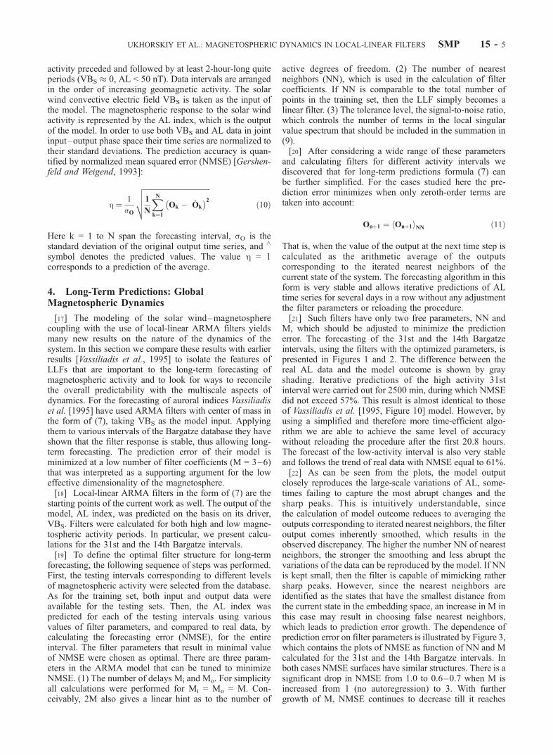
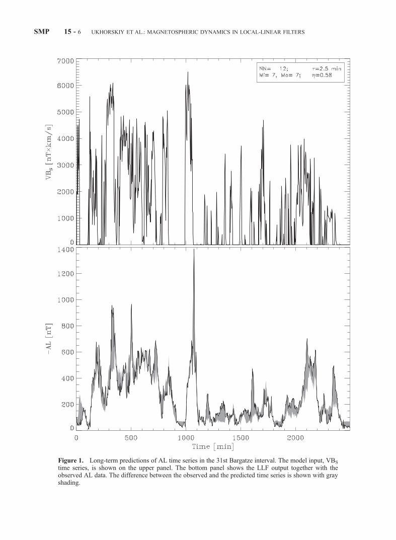
M, which should be adjusted to minimize the predictionerror. The forecasting of the 31st and the 14th Bargatzeintervals, using the filters with the optimized parameters, ispresented in Figures 1 and 2. The difference between thereal AL data and the model outcome is shown by grayshading. Iterative predictions of the high activity 31stinterval were carried out for 2500 min, during which NMSEdid not exceed 57%. This result is almost identical to thoseof Vassiliadis et al. [1995, Figure 10] model. However, byusing a simplified and therefore more time-efficient algo-rithm we are able to achieve the same level of accuracywithout reloading the procedure after the first 20.8 hours.The forecast of the low-activity interval is also very stableand follows the trend of real data with NMSE equal to 61%.[22] As can be seen from the plots, the model output

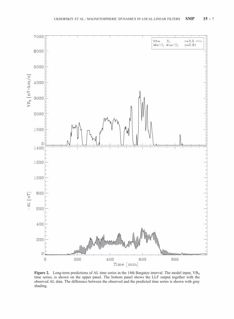
closely reproduces the large-scale variations of AL, some-times failing to capture the most abrupt changes and thesharp peaks. This is intuitively understandable, sincethe calculation of model outcome reduces to averaging theoutputs corresponding to iterated nearest neighbors, the filteroutput comes inherently smoothed, which results in theobserved discrepancy. The higher the number NN of nearestneighbors, the stronger the smoothing and less abrupt thevariations of the data can be reproduced by the model. If NNis kept small, then the filter is capable of mimicking rathersharp peaks. However, since the nearest neighbors areidentified as the states that have the smallest distance fromthe current state in the embedding space, an increase in M inthis case may result in choosing false nearest neighbors,which leads to prediction error growth. The dependence ofprediction error on filter parameters is illustrated by Figure 3,which contains the plots of NMSE as function of NN and Mcalculated for the 31st and the 14th Bargatze intervals. Inboth cases NMSE surfaces have similar structures. There is asignificant drop in NMSE from 1.0 to 0.6–0.7 when M isincreased from 1 (no autoregression) to 3. With furthergrowth of M, NMSE continues to decrease till it reaches


Figure 1. Long-term predictions of AL time series in the 31st Bargatze interval. The model input, VBS

time series, is shown on the upper panel. The bottom panel shows the LLF output together with theobserved AL data. The difference between the observed and the predicted time series is shown with grayshading.


Figure 2. Long-term predictions of AL time series in the 14th Bargatze interval. The model input, VBS

time series, is shown on the upper panel. The bottom panel shows the LLF output together with theobserved AL data. The difference between the observed and the predicted time series is shown with grayshading.


its minimum. For the high activity interval the smallestNMSE values are observed for 2M � NN = 14. In the caseof low activity, NMSE has several local minima, one ofwhich (M = 10, N = 5) was chosen for the demonstration run(Figure 2). With further increase in either of filter parametersNMSE starts to grow again. For high NN values it saturates,which indicates that the filter becomes effectively linear. Forlow NN values, when M increases NMSE grows fast till itreaches 1.0 again. The overall structure of NMSE surfacesshown in Figure 3 is very similar to the error surfacespresented by Vassiliadis et al. [1995, Figure 12], excepttheir prediction error reaches its minimum at lower M values(2–3) and higher NN values (�30).[23] If linear terms are included in LLF expression, then

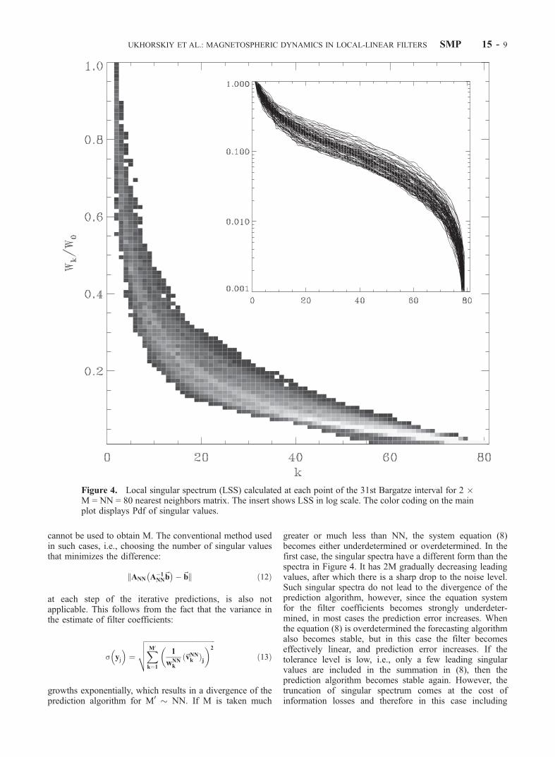
the filter response can significantly change, depending on itsparameters. If the tolerance level is high, that is a widerange of perturbation scales is taken into account in (9), and2M � NN the algorithm becomes unstable and divergesafter a few steps. This behavior of the filter outcome can beaccounted for by the form of singular value spectrum

obtained from the nearest neighbors matrix. Unlike theglobal singular spectrum, which has a power law shape,local singular spectrum has a steeper exponential form. Theresult of local singular spectrum calculations for the 31stBargatze interval is shown in Figure 4. The spectra werecalculated for the set of 80 nearest neighbors at each pointof the interval. As can be seen from the plot all spectra aresimilar in form. The spectra consist of the main exponentialpart, which is preceded and followed by the shorter intervalsof steeper drop. Moreover, singular values calculated fordifferent points of the interval and therefore correspondingto different levels of substorm activity are very similar. Thisfact may be interpreted as an indication of self-similarity ofthe attractor that underlies the system dynamics.[24] In spite of its steepness, the form of the local singular

spectra alone does not yield the number of delays Mrequired to embed the underlying phase space. Indeed, thespectra retain their form over the wide range of scales(10�3 < wk/w0 < 1) without a noise plateau, and conse-quently the prescription of Broomhead and King [1986]

Figure 3. The prediction error (NMSE) of the mean-field model is plotted as a function of the numberof nearest neighbors (NN) and the number of delays (M). Error surfaces are plotted for AL predictions inthe 31st (a) and 14th (c) Bargatze intervals. To provide a better view on their inner parts, the samesurfaces are replotted for the narrower M range ((b) and (d)), starting from M = 4 instead of M = 1.


cannot be used to obtain M. The conventional method usedin such cases, i.e., choosing the number of singular valuesthat minimizes the difference:

kANN A�1NN~b

� ��~bk ð12Þ

at each step of the iterative predictions, is also notapplicable. This follows from the fact that the variance inthe estimate of filter coefficients:

s yj

� �¼

ffiffiffiffiffiffiffiffiffiffiffiffiffiffiffiffiffiffiffiffiffiffiffiffiffiffiffiffiffiffiffiffiffiffiffiffiffiffiffiXM0

k¼1

1

wNNk

~vNNkð Þj� 2

vuut ð13Þ

growths exponentially, which results in a divergence of theprediction algorithm for M0 � NN. If M is taken much

greater or much less than NN, the system equation (8)becomes either underdetermined or overdetermined. In thefirst case, the singular spectra have a different form than thespectra in Figure 4. It has 2M gradually decreasing leadingvalues, after which there is a sharp drop to the noise level.Such singular spectra do not lead to the divergence of theprediction algorithm, however, since the equation systemfor the filter coefficients becomes strongly underdeter-mined, in most cases the prediction error increases. Whenthe equation (8) is overdetermined the forecasting algorithmalso becomes stable, but in this case the filter becomeseffectively linear, and prediction error increases. If thetolerance level is low, i.e., only a few leading singularvalues are included in the summation in (8), then theprediction algorithm becomes stable again. However, thetruncation of singular spectrum comes at the cost ofinformation losses and therefore in this case including

Figure 4. Local singular spectrum (LSS) calculated at each point of the 31st Bargatze interval for 2 �M = NN = 80 nearest neighbors matrix. The insert shows LSS in log scale. The color coding on the mainplot displays Pdf of singular values.


linear terms in the model does not improve the predict-ability. On the contrary in most cases this leads to anincrease in forecasting error.[25] Consequently, for the long-term forecasting of AL

time series the linear terms in the expression for conven-tional local-linear ARMA filters can be omitted. In thiscase the entire prediction procedure reduces to finding themean-field response of the system, i.e., the averageresponse of the similar states of the system in thereconstructed input–output phase space. The mean-fieldmodel output closely follows the trend of AL data duringboth high and low magnetospheric activity, reproducingbest of all the large-scale variations. Thus, the mean-fieldmodel naturally represents the large-scale component ofthe AL dynamics. Being regular and predictable, it corre-sponds to the globally coherent features of the magneto-spheric dynamics during substorms. Moreover, since thenumber of delays M is directly related to the effectivedimension of the system, the results indicate that theglobal component of the magnetospheric dynamics hasfinite dimension.

5. Data Reconstruction: Multiscale Aspects ofMagnetospheric Dynamics

[26] The mean-field approach to solar wind–magneto-sphere coupling, described in the previous section, providesa framework for modeling the large-scale or global dynam-ics, for example as represented by AL time series, and forbuilding a framework for space weather forecasting tools.However, the inability to capture the sporadic peaks andabrupt variations in the data may limit the utility of thetechnique as a space weather forecasting tool.[27] The inability of the model to yield more accurate

forecasts is due to the divergence of the standard predictionalgorithm, when a wider range of singular values is consid-ered in the computation of the LLFs. The singular spectrumis analogous to a Fourier spectrum, and the singular valuesare nothing but the coefficients that weigh the contribution ofcertain scale perturbations in the observed time series. Thus,the truncation of the singular spectrum, dictated by algorithmstability issues, limits the range of perturbation scales.Moreover, due to the algorithm divergence it is not evenclear what this range is, or whether it is finite or not. Thisissue is of great importance for understanding the dynamicalproperties of the system as well as for developing moreaccurate forecasting tools. Indeed, if the range of perturba-tion scales that are inherent in the observed time series is notfinite, then since it is directly related to the number of activedimensions, there is no finite dimensional space that pro-vides a proper embedding for the system. This means that thedynamics of the system is not deterministic and the predict-ability of its evolution is limited to that of the mean-fieldmodel. On the other hand, if the range of perturbation scalesis finite and can be somehow determined at each step of theiterative predictions, then including the higher-order terms infilter expression can significantly increase the predictionaccuracy.[28] This is an important issue for space weather fore-

casting and it can be addressed with use of local-linearARMA filters in the form given by equation (7). For thispurpose, instead of making the iterative predictions of AL

for some testing interval and then minimizing the predic-tion error by adjusting the filter parameters, and thetolerance level for the whole prediction interval, filterscan be used in an inverse problem manner. That is, bycomparing the filter outcome with real data at each step ofiterative predictions, the number of terms M0 of localsingular spectrum that gives rise to the observed AL timeseries (see (9)) can be determined. Presumably, this proce-dure, which will be referred as data reconstruction, shouldreturn the different number M0 at each time step. It isexpected that in the case of low-dimensional system M0

should oscillate around the mean value M*, which givesthe linear estimate of the system dimensionality. However,in the case of a system which has a significant high-dimensional multiscale component, M0 should have asporadic distribution, i.e., M0 should be evenly distributedfrom 1 to 2M, the total number of input–output embeddingspace dimensions, no matter how big is M. This indicatesthat the observed time series consist of perturbations of awide range of scales.[29] To elucidate these properties in the case of solar

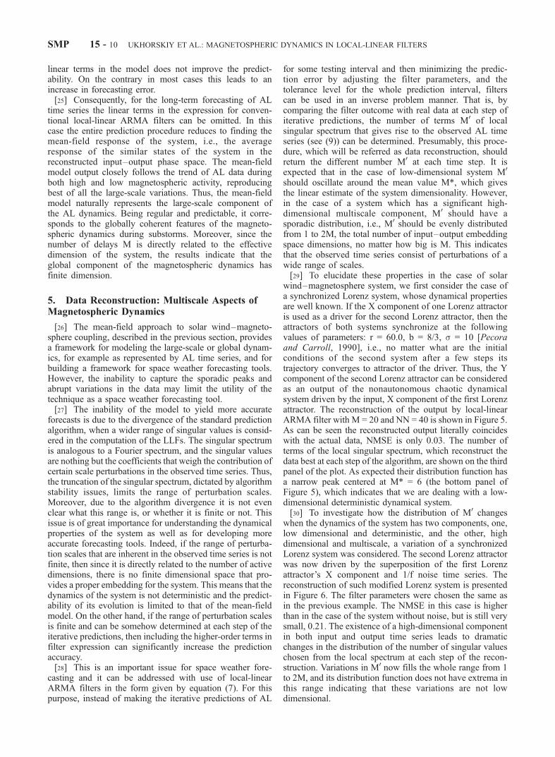
wind–magnetosphere system, we first consider the case ofa synchronized Lorenz system, whose dynamical propertiesare well known. If the X component of one Lorenz attractoris used as a driver for the second Lorenz attractor, then theattractors of both systems synchronize at the followingvalues of parameters: r = 60.0, b = 8/3, s = 10 [Pecoraand Carroll, 1990], i.e., no matter what are the initialconditions of the second system after a few steps itstrajectory converges to attractor of the driver. Thus, the Ycomponent of the second Lorenz attractor can be consideredas an output of the nonautonomous chaotic dynamicalsystem driven by the input, X component of the first Lorenzattractor. The reconstruction of the output by local-linearARMA filter with M = 20 and NN = 40 is shown in Figure 5.As can be seen the reconstructed output literally coincideswith the actual data, NMSE is only 0.03. The number ofterms of the local singular spectrum, which reconstruct thedata best at each step of the algorithm, are shown on the thirdpanel of the plot. As expected their distribution function hasa narrow peak centered at M* = 6 (the bottom panel ofFigure 5), which indicates that we are dealing with a low-dimensional deterministic dynamical system.[30] To investigate how the distribution of M0 changes

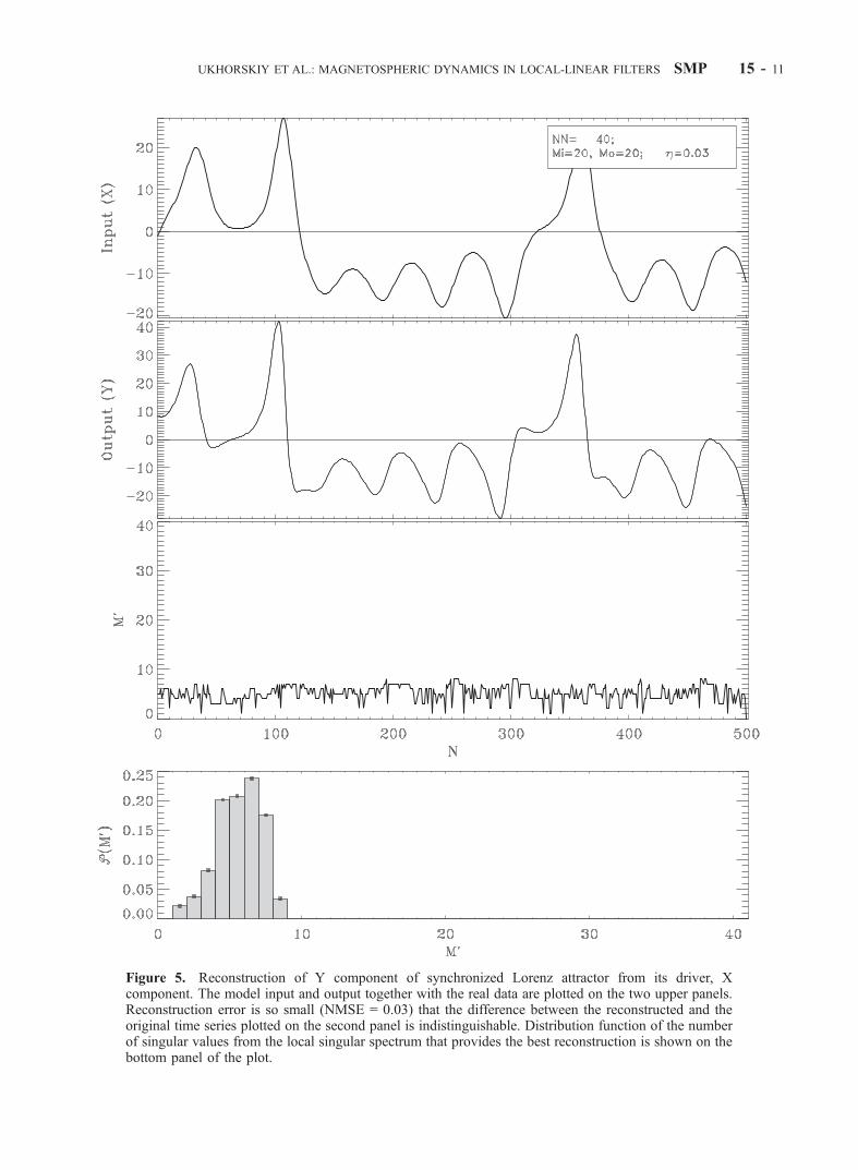
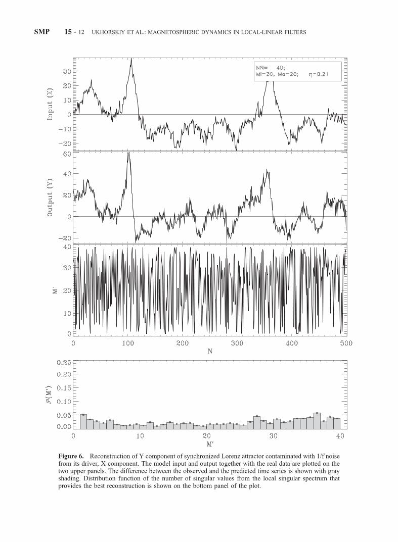
when the dynamics of the system has two components, one,low dimensional and deterministic, and the other, highdimensional and multiscale, a variation of a synchronizedLorenz system was considered. The second Lorenz attractorwas now driven by the superposition of the first Lorenzattractor’s X component and 1/f noise time series. Thereconstruction of such modified Lorenz system is presentedin Figure 6. The filter parameters were chosen the same asin the previous example. The NMSE in this case is higherthan in the case of the system without noise, but is still verysmall, 0.21. The existence of a high-dimensional componentin both input and output time series leads to dramaticchanges in the distribution of the number of singular valueschosen from the local spectrum at each step of the recon-struction. Variations in M0 now fills the whole range from 1to 2M, and its distribution function does not have extrema inthis range indicating that these variations are not lowdimensional.


Figure 5. Reconstruction of Y component of synchronized Lorenz attractor from its driver, Xcomponent. The model input and output together with the real data are plotted on the two upper panels.Reconstruction error is so small (NMSE = 0.03) that the difference between the reconstructed and theoriginal time series plotted on the second panel is indistinguishable. Distribution function of the numberof singular values from the local singular spectrum that provides the best reconstruction is shown on thebottom panel of the plot.


Figure 6. Reconstruction of Y component of synchronized Lorenz attractor contaminated with 1/f noisefrom its driver, X component. The model input and output together with the real data are plotted on thetwo upper panels. The difference between the observed and the predicted time series is shown with grayshading. Distribution function of the number of singular values from the local singular spectrum thatprovides the best reconstruction is shown on the bottom panel of the plot.


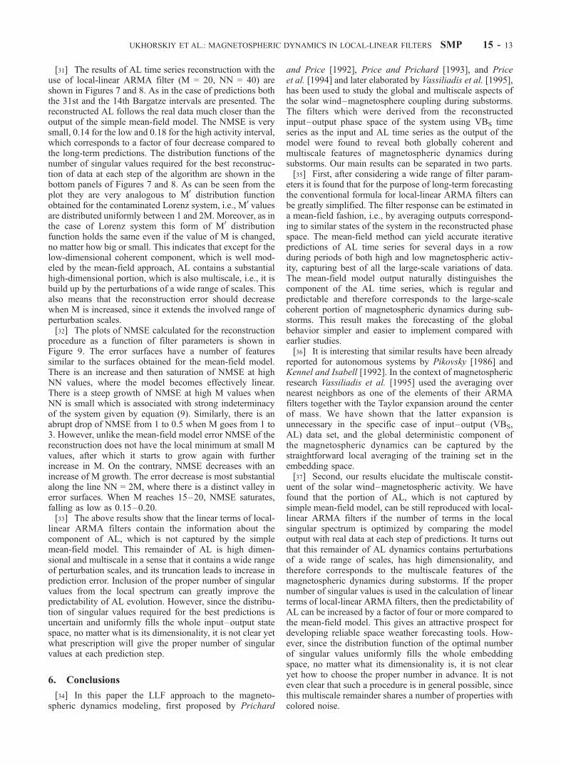
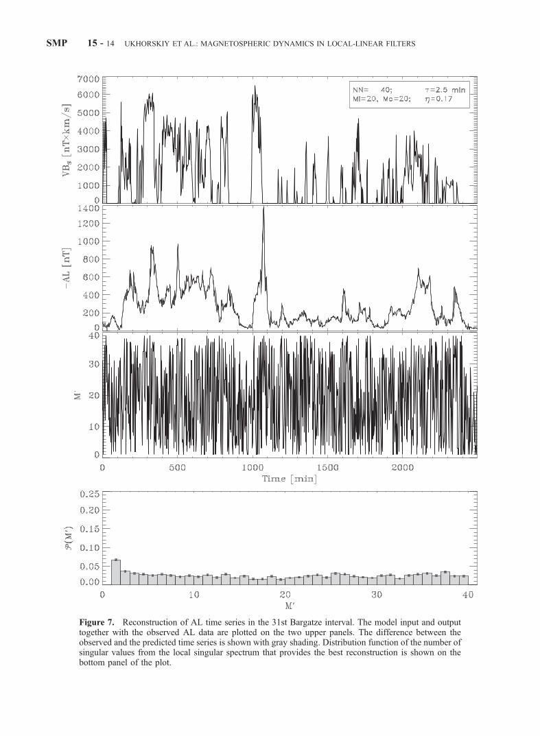
[31] The results of AL time series reconstruction with theuse of local-linear ARMA filter (M = 20, NN = 40) areshown in Figures 7 and 8. As in the case of predictions boththe 31st and the 14th Bargatze intervals are presented. Thereconstructed AL follows the real data much closer than theoutput of the simple mean-field model. The NMSE is verysmall, 0.14 for the low and 0.18 for the high activity interval,which corresponds to a factor of four decrease compared tothe long-term predictions. The distribution functions of thenumber of singular values required for the best reconstruc-tion of data at each step of the algorithm are shown in thebottom panels of Figures 7 and 8. As can be seen from theplot they are very analogous to M0 distribution functionobtained for the contaminated Lorenz system, i.e., M0 valuesare distributed uniformly between 1 and 2M. Moreover, as inthe case of Lorenz system this form of M0 distributionfunction holds the same even if the value of M is changed,no matter how big or small. This indicates that except for thelow-dimensional coherent component, which is well mod-eled by the mean-field approach, AL contains a substantialhigh-dimensional portion, which is also multiscale, i.e., it isbuild up by the perturbations of a wide range of scales. Thisalso means that the reconstruction error should decreasewhen M is increased, since it extends the involved range ofperturbation scales.[32] The plots of NMSE calculated for the reconstruction

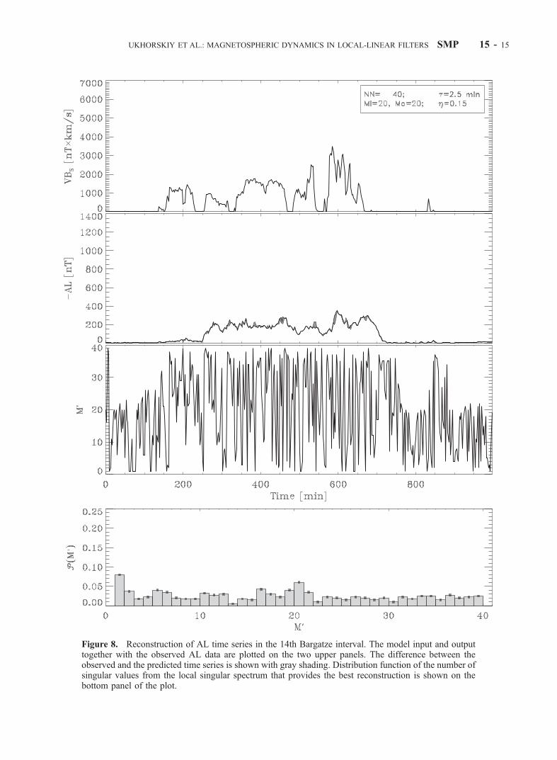
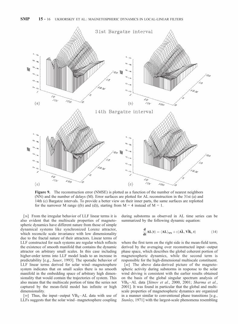
procedure as a function of filter parameters is shown inFigure 9. The error surfaces have a number of featuressimilar to the surfaces obtained for the mean-field model.There is an increase and then saturation of NMSE at highNN values, where the model becomes effectively linear.There is a steep growth of NMSE at high M values whenNN is small which is associated with strong indeterminacyof the system given by equation (9). Similarly, there is anabrupt drop of NMSE from 1 to 0.5 when M goes from 1 to3. However, unlike the mean-field model error NMSE of thereconstruction does not have the local minimum at small Mvalues, after which it starts to grow again with furtherincrease in M. On the contrary, NMSE decreases with anincrease of M growth. The error decrease is most substantialalong the line NN = 2M, where there is a distinct valley inerror surfaces. When M reaches 15–20, NMSE saturates,falling as low as 0.15–0.20.[33] The above results show that the linear terms of local-

linear ARMA filters contain the information about thecomponent of AL, which is not captured by the simplemean-field model. This remainder of AL is high dimen-sional and multiscale in a sense that it contains a wide rangeof perturbation scales, and its truncation leads to increase inprediction error. Inclusion of the proper number of singularvalues from the local spectrum can greatly improve thepredictability of AL evolution. However, since the distribu-tion of singular values required for the best predictions isuncertain and uniformly fills the whole input–output statespace, no matter what is its dimensionality, it is not clear yetwhat prescription will give the proper number of singularvalues at each prediction step.

6. Conclusions

[34] In this paper the LLF approach to the magneto-spheric dynamics modeling, first proposed by Prichard

and Price [1992], Price and Prichard [1993], and Priceet al. [1994] and later elaborated by Vassiliadis et al. [1995],has been used to study the global and multiscale aspects ofthe solar wind–magnetosphere coupling during substorms.The filters which were derived from the reconstructedinput–output phase space of the system using VBS timeseries as the input and AL time series as the output of themodel were found to reveal both globally coherent andmultiscale features of magnetospheric dynamics duringsubstorms. Our main results can be separated in two parts.[35] First, after considering a wide range of filter param-

eters it is found that for the purpose of long-term forecastingthe conventional formula for local-linear ARMA filters canbe greatly simplified. The filter response can be estimated ina mean-field fashion, i.e., by averaging outputs correspond-ing to similar states of the system in the reconstructed phasespace. The mean-field method can yield accurate iterativepredictions of AL time series for several days in a rowduring periods of both high and low magnetospheric activ-ity, capturing best of all the large-scale variations of data.The mean-field model output naturally distinguishes thecomponent of the AL time series, which is regular andpredictable and therefore corresponds to the large-scalecoherent portion of magnetospheric dynamics during sub-storms. This result makes the forecasting of the globalbehavior simpler and easier to implement compared withearlier studies.[36] It is interesting that similar results have been already

reported for autonomous systems by Pikovsky [1986] andKennel and Isabell [1992]. In the context of magnetosphericresearch Vassiliadis et al. [1995] used the averaging overnearest neighbors as one of the elements of their ARMAfilters together with the Taylor expansion around the centerof mass. We have shown that the latter expansion isunnecessary in the specific case of input–output (VBS,AL) data set, and the global deterministic component ofthe magnetospheric dynamics can be captured by thestraightforward local averaging of the training set in theembedding space.[37] Second, our results elucidate the multiscale constit-

uent of the solar wind–magnetospheric activity. We havefound that the portion of AL, which is not captured bysimple mean-field model, can be still reproduced with local-linear ARMA filters if the number of terms in the localsingular spectrum is optimized by comparing the modeloutput with real data at each step of predictions. It turns outthat this remainder of AL dynamics contains perturbationsof a wide range of scales, has high dimensionality, andtherefore corresponds to the multiscale features of themagnetospheric dynamics during substorms. If the propernumber of singular values is used in the calculation of linearterms of local-linear ARMA filters, then the predictability ofAL can be increased by a factor of four or more compared tothe mean-field model. This gives an attractive prospect fordeveloping reliable space weather forecasting tools. How-ever, since the distribution function of the optimal numberof singular values uniformly fills the whole embeddingspace, no matter what its dimensionality is, it is not clearyet how to choose the proper number in advance. It is noteven clear that such a procedure is in general possible, sincethis multiscale remainder shares a number of properties withcolored noise.


Figure 7. Reconstruction of AL time series in the 31st Bargatze interval. The model input and outputtogether with the observed AL data are plotted on the two upper panels. The difference between theobserved and the predicted time series is shown with gray shading. Distribution function of the number ofsingular values from the local singular spectrum that provides the best reconstruction is shown on thebottom panel of the plot.


Figure 8. Reconstruction of AL time series in the 14th Bargatze interval. The model input and outputtogether with the observed AL data are plotted on the two upper panels. The difference between theobserved and the predicted time series is shown with gray shading. Distribution function of the number ofsingular values from the local singular spectrum that provides the best reconstruction is shown on thebottom panel of the plot.


[38] From the irregular behavior of LLF linear terms it isalso evident that the multiscale properties of magneto-spheric dynamics have different nature from those of simpledynamical systems like synchronized Lorenz attractor,which reconcile scale invariance with low dimensionalitydue to the fractal nature of their attractors. Linear terms ofLLF constructed for such systems are regular which reflectsthe existence of smooth manifold that contains the dynamicattractor on arbitrary small scales. In this case includinghigher-order terms into LLF model leads to an increase inpredictability [e.g., Sauer, 1993]. The sporadic behavior ofLLF linear terms derived for solar wind–magnetospheresystem indicates that on small scales there is no smoothmanifold in the embedding space of arbitrary high dimen-sionality that would contain the trajectories of system. Thisalso means that the multiscale portion of time the series notcaptured by the mean-field model has infinite or highdimensionality.[39] Thus, the input–output VBS–AL data with use of

LLFs suggests that the solar wind–magnetosphere coupling

during substorms as observed in AL time series can besummarized by the following dynamic equation:

d

dtAL tð Þ ¼ ALh iNN þ eð ~AL; ~VBs; tÞ ð14Þ

where the first term on the right side is the mean-field term,derived by the averaging over reconstructed input–outputphase space, which describes the global coherent portion ofmagnetospheric dynamics, while the second term isresponsible for the high-dimensional multiscale constituent.[40] The above data-derived picture of the magneto-

spheric activity during substorms in response to the solarwind driving is consistent with the earlier results obtainedon the basis of the global singular spectrum analysis ofVBS–AL data [Sitnov et al., 2000, 2001; Sharma et al.,2001]. It was found in particular that the global and multi-scale properties of magnetospheric dynamics are organizedin a manner similar to conventional phase transitions [e.g.,Stanley, 1971] with the largest-scale phenomena resembling

Figure 9. The reconstruction error (NMSE) is plotted as a function of the number of nearest neighbors(NN) and the number of delays (M). Error surfaces are plotted for AL reconstruction in the 31st (a) and14th (c) Bargatze intervals. To provide a better view on their inner parts, the same surfaces are replottedfor the narrower M range ((b) and (d)), starting from M = 4 instead of M = 1.


first-order phase transitions in the mean-field approxima-tion, while the multiscale constituent having properties ofsecond-order transitions near the critical point. The first-order transition picture of the magnetosphere was obtainedin the three leading principal components corresponding tothe largest eigenvalues of the correlation matrix with addi-tional local averaging in that 3D space. The averagedynamics of the magnetosphere is then similar to the regularmotion on a folded surface like the ‘‘temperature–pres-sure–density’’ diagram of dynamical phase transitions [e.g.,Gunton et al., 1983] or the cusp catastrophe manifold[Lewis, 1991]. Our present results strongly support such adescription of the mean-field picture. On the other hand, theresults of the global singular spectrum analysis suggest thatthe multiscale constituent of the magnetospheric activitymay be neither a colored noise independent of the solarwind properties as suggested in the models of magneto-spheric turbulence [e.g., Borovsky et al., 1993, 1997] andSOC [e.g., Consolini, 1997; Chapman et al., 1998; Uritskyand Pudovkin, 1998; Lui et al., 2000], nor a direct reflectionof the appropriate multiscale solar wind properties assuggested by Freeman et al. [2000]. It can rather be viewedas the multiscale response involving both input and outputparameters as is reflected by input–output critical expo-nents similar to those of the second-order phase transitions[Sitnov et al., 2001]. Therefore, further improvement in thepredictability may be achieved by a combination of thedynamical description for the global component and astatistical approach for the multiscale component, by study-ing its correlation with the solar wind input.

[41] Acknowledgments. We thank D. Vassiliadis for many fruitfuldiscussions. The research is supported by NSF grants ATM-0001676 andATM-0119196 and NASA grant NAG5-1101.

ReferencesAbarbanel, H. D., R. Brown, J. J. Sidorovich, and T. S. Tsimring, Theanalysis of observed chaotic data in physical systems, Rev. Mod. Phys.,65, 1331, 1993.

Angelopoulos, V., T. Mukai, and S. Kokubun, Evidence for intermittency inEarth’s plasma sheet and implications for self-organized criticality, Phys.Plasmas, 6, 4161, 1999.

Bak, P., C. Tang, and K. Wiesenfeld, Self-organized criticality: An explana-tion of 1/f noise, Phys. Rev. Lett., 59, 381, 1987.

Bargatze, L. F., D. N. Baker, R. L. McPherron, and E. W. Hones, Magneto-spheric impulse response for many levels of geomagnetic activity,J. Geophys. Res., 90, 6387, 1985.

Borovsky, J. E., R. J. Nemzek, and R. D. Belian, The occurrence rate ofmagnetospheric-substorm onsets: Random and periodic substorms,J. Geophys. Res., 98, 3807, 1993.

Borovsky, J. E., R. C. Elphic, H. O. Funsten, and M. F. Thomsen, TheEarth’s plasma sheet as a laboratory for flow turbulence in high-b MHD,J. Plasma Phys., 57, 1, 1997.

Broomhead, D. S., and G. P. King, Extracting qualitative dynamics fromexperimental data, Physica D, 20, 217, 1986.

Casdagli, M., Nonlinear prediction of chaotic time series, Physica D, 35,335, 1989.

Casdagli, M., A dynamical approach to modeling input–output systems, inNonlinear Modeling and Forecasting, edited by M. Casdagli and S. Eu-bank, p. 265, Addison-Wesley-Longman, Reading, Mass., 1992.

Chakrabarti, B. K., and M. Acharyya, Dynamic transitions and hysteresis,Rev. Mod. Phys., 71, 847, 1999.

Chang, T., Multiscale intermittent turbulence in the magnetotail, in SUB-STORMS-4, edited by S. Kokubun and Y. Kamide, p. 431, Terra Sci.,Tokyo, 1998.

Chang, T., Self-organized criticality, multi-fractal spectra, sporadic loca-lized reconnections and intermittent turbulence in the magnetotail, Phys.Plasmas, 6, 4137–4145, 1999.

Chapman, S. C., N. W. Watkins, R. O. Dendy, P. Helander, and G. Row-

lands, A simple avalanche model as an analogue for magnetosphericactivity, Geophys. Res. Lett., 25, 2397, 1998.

Consolini, G., Sandpile cellular automata and magnetospheric dynamics,in Proceeding of the 8th GIFCO Conference, Cosmic Physics in theYear 2000: Scientific Perspectives and New Instrumentation, 8 –10April 1997, edited by S. Aiello et al., Soc. Ital. di Fis., Bologna, Italy,pp. 123–126, 1997.

Consolini, G., M. F. Marcucci, and M. Candidi, Multifractal structure ofauroral electrojet index data, Phys. Rev. Lett., 76, 4082, 1996.

Detman, T. R., and D. Vassiliadis, Review of techniques of the magneticstorm forecasting, in Magnetic Storms, Geophys. Monogr. Ser., vol. 98,edited by B. T. Tsurutani et al., pp. 253–266, AGU, Washington, D. C.,1997.

Farmer, J. D., and J. J. Sidorowich, Predicting chaotic time series, Phys.Rev. Lett., 59, 845, 1987.

Freeman, M. P., N. W. Watkins, and D. J. Riley, Evidence for solar windorigin of the power law burst lifetime distribution of the AE indices,Geophys. Res. Lett., 27, 1087, 2000.

Gershenfeld, N. A., and A. S. Weigend, The future of time series: Learningand understanding, in Time Series Prediction: Forecasting the Future andUnderstanding the Past, Santa Fe Inst. Stud. in the Sci. of ComplexityXV, edited by A. S. Weigend and N. A. Gershenfeld, pp. 1–70, Addison-Wesley-Longman, Reading, Mass., 1993.

Grassberger, P., and I. Procaccia, Measuring the strangeness of strangeattractors, Physica D, 9, 189, 1983.

Gunton, J. D., M. S. Miguel, and P. S. Sahni, The dynamics of first-orderphase transitions, in Phase Transitions, Volume 8, p. 267, Academic, SanDiego, Calif., 1983.

Hohenberg, P. C., and B. I. Halperin, Theory of dynamic critical phenom-ena, Rev. Mod. Phys., 49, 435, 1977.

Ieda, A., S. Mashida, T. Mukai, Y. Saito, T. Yamamoto, A. Nishida,T. Terasawa, and S. Kokubun, Statistical analysis of the plasmoid evolu-tion with Geotail observations, J. Geophys. Res., 103, 4453, 1998.

Kennel, M. B., and S. Isabell, Method to distinguish possible chaos fromcolored noise and to determine embedding parameters, Phys. Rev. A, 46,3111, 1992.

Klimas, A. J., D. N. Baker, D. A. Roberts, D. H. Fairfield, and J. Buchner,A nonlinear dynamical analogue model of geomagnetic activity, J. Geo-phys. Res., 97, 12,253, 1992.

Klimas, A. J., D. Vassiliadis, D. A. Roberts, and D. N. Baker, The orga-nized nonlinear dynamics of the magnetosphere (an invited review),J. Geophys. Res., 101, 13,089, 1996.

Klimas, A. J., J. A. Valdivia, D. Vassiliadis, D. N. Baker, M. Hesse, andJ. Takalo, Self-organized criticality in the substorm phenomenon and itsrelation to localized reconnection in the magnetospheric plasma sheet,J. Geophys. Res., 105, 18,765, 2000.

Lewis, Z. V., On the apparent randomness of substorm onset, Geophys. Res.Lett., 18, 1627, 1991.

Lui, A. T. Y., A. C. Chapman, K. Liou, P. T. Newell, C. I. Meng,M. Brittnacher, and G. K. Parks, Is the dynamic of magnetosphere anavalanching system?, Geophys. Res. Lett., 27, 911, 2000.

Nagai, T., M. Fujimoto, Y. Saito, S. Mashida, T. Terasawa, R. Nakamura,T. Yamamoto, T. Mukai, A. Nishida, and S. Kokubun, Structure anddynamics of magnetic reconnection for substorm onsets with Geotailobservations, J. Geophys. Res., 103, 4419, 1998.

Nagel, S. R., Instabilities in a sandpile, Rev. Mod. Phys., 64, 321–325,1992.

Ohtani, S., T. Higuchi, A. T. Lui, and K. Takahashi, Magnetic fluctuationsassociated with tail current disruption: Fractal analysis, J. Geophys. Res.,100, 19,135, 1995.

Packard, N., J. Crutchfield, D. Farmer, and R. Shaw, Geometry from a timeseries, Phys. Rev. Lett., 45, 712, 1980.

Pecora, L. M., and T. L. Carroll, Synchronization in chaotic systems, Phys.Rev. Lett., 64, 821, 1990.

Petrukovich, A. A., et al., Two spacecraft observations of a reconnectionpulse during an auroral breakup, J. Geophys. Res., 103, 47, 1998.

Pikovsky, A., Noise filtering in the discrete time dynamical systems, Sov. J.Commun. Technol. Electron., 31, 911, 1986.

Price, C. P., and D. Prichard, The nonlinear response of the magnetosphere:30 October 1978, Geophys. Res. Lett., 20, 771, 1993.

Price, C. P., D. Prichard, and J. E. Bischoff, Non-linear input/output ana-lysis of the auroral electrojet index, J. Geophys. Res., 99, 13,227, 1994.

Prichard, D., and C. P. Price, Is the AE index the result of nonlineardynamics?, Geophys. Res. Lett., 20, 2817, 1992.

Prichard, D., J. E. Borovsky, P. M. Lemons, and C. P. Price, Time depen-dence of substorm recurrence: An information theoretic analysis, J. Geo-phys. Res., 101, 15,359, 1996.

Sauer, T., Time series prediction by using delay coordinate embedding, inTime Series Prediction: Forecasting the Future and Understanding thePast, Santa Fe Inst. Stud. in the Sci. of Complexity XV, edited by A. S.


Weigend and N. A. Gershenfeld, pp. 175–193, Addison-Wesley-Long-man, Reading, Mass., 1993.

Sauer, T., J. A. Yorke, and M. Casdagli, Embedology, J. Stat. Phys., 65,579, 1991.

Sharma, A. S., Assessing the magnetosphere’s nonlinear behavior: Its di-mension is low, its predictability high (US National Report to IUGG,1991–1994), Rev. Geophys. Suppl., 33, 645–650, 1995.

Sharma, A. S., D. Vassiliadis, and K. Papadopoulos, Reconstruction of lowdimensional magnetospheric dynamics by singular spectrum analysis,Geophys. Res. Lett., 20, 335, 1993.

Sharma, A. S., M. I. Sitnov, and K. Papadopoulos, Substorms as none-quilibrium transitions in the magnetosphere, J. Atmos. Sol. Terr. Phys.,63, 1399, 2001.

Sitnov, M. I., A. S. Sharma, K. Papadopoulos, D. Vassiliadis, J. A. Valdivia,A. J. Klimas, and D. N. Baker, Phase transition-like behavior of themagnetosphere during substorms, J. Geophys. Res., 105, 12,955, 2000.

Sitnov, M. I., A. S. Sharma, K. Papadopoulos, and D. Vassiliadis, Modelingsubstorm dynamics of the magnetosphere: From self-organization andself-criticality to nonequilibrium phase transitions, Phys. Rev. E., 65,16,116, 2001.

Smith, A. J., M. P. Freeman, and G. D. Reeves, Postmidnight VLF chorusevents, a substorm signature observed at the ground near L = 4,J. Geophys. Res., 101, 24,641, 1996.

Stanley, H. E., Introduction to Phase Transition and Critical Phenomena,Oxford Univ. Press, New York, 1971.

Takalo, J., J. Timonen, and H. Koskinen, Correlation dimension and affinityof AE data and bicolored noise, Geophys. Res. Lett., 20, 1527, 1993.

Takalo, J., J. Timonen, and H. Koskinen, Properties of AE data and bico-lored noise, J. Geophys. Res., 99, 13,239, 1994.

Takalo, J., J. Timonen, A. J. Klimas, J. A. Valdivia, and D. Vassiliadis,Nonlinear energy dissipation in a cellular automation magnetotail model,Geophys. Res. Lett., 26, 1813, 1999.

Takens, F., Detecting strange attractors in fluid turbulence, in DynamicalSystems and Turbulence, edited by D. Rand and L. S. Young, pp. 366–381, Springer-Verlag, New York, 1981.

Theiler, J., Some comments on the correlation dimension of 1/f a noise,Phys. Lett. A, 155, 480, 1991.

Tsurutani, B. T., M. Sugiura, T. Iyemori, B. E. Goldstein, W. D. Gonzalez,S. I. Akasofu, and E. J. Smith, The nonlinear response of AE to the IMFBs driver: A spectral break at 5 hours, Geophys. Res. Lett., 17, 279, 1990.

Uritsky, V. M., and M. I. Pudovkin, Low frequency 1/f-like fluctuations ofthe AE-index as a possible manifestation of self-organized criticality inthe magnetosphere, Ann. Geophys., 16(12), 1580, 1998.

Valdivia, J. A., A. S. Sharma, and K. Papadopoulos, Prediction of magneticstorms with nonlinear dynamical models, Geophys. Res. Lett., 23, 2899,1996.

Vassiliadis, D., A. S. Sharma, T. E. Eastman, and K. Papadopoulos, Lowdimensional chaos in magnetospheric activity from AE time series, Geo-phys. Res. Lett., 17, 1841, 1990.

Vassiliadis, D., A. J. Klimas, D. B. Baker, and D. A. Roberts, A descriptionof the solar wind–magnetosphere coupling based on nonlinear filters,J. Geophys. Res., 100, 3495, 1995.

Vespignani, A., and S. Zapperi, How self-organized criticality works: Aunified mean-field picture, Phys. Rev. E, 57, 6345, 1998.

Watkins, N. W., S. C. Chapman, R. O. Dendy, and G. Rowlands, Robust-ness of collective behaviour in strongly driven avalanche models: Mag-netospheric implications, Geophys. Res. Lett., 26, 2617, 1999.

Zheng, B., M. Schulz, and S. Trimper, Deterministic equations of motionand dynamic critical phenomena, Phys. Rev. Lett., 82, 1891, 1999.

��K. Papadopoulos, A. S. Sharma, M. I. Sitnov, and A. Y. Ukhorskiy,

Department of Physics, University of Maryland at College Park, CollegePark, MD, USA.


Date post:	16-Aug-2019
Category:	Documents
Upload:	dangnga
View:	214 times
Download:	0 times

Global and multiscale aspects of magnetospheric dynamics...

Documents