20
Global Climate Destabilization: Optimal Opportunity for the Mathematics of Planet Earth Andrew Long Northern Kentucky University Joint Math Meetings San Diego, CA 2013
| Date post: | 26-Dec-2015 |
| Category: |
Documents |
| Upload: | phyllis-preston |
| View: | 214 times |
| Download: | 0 times |

Global Climate Destabilization:
Optimal Opportunity for the Mathematics of Planet Earth
Andrew LongNorthern Kentucky University
Joint Math MeetingsSan Diego, CA
2013

Global Climate Destabilization (GCD) : There’s good news and bad news….
• Bad news first: destabilization is occurring, and is ominous. Are there any silver linings?”
• Good news: GCD is an interesting and engaging context for studying math. Why? – There is a bountiful variety of topics to choose from. – Graphics and data abound, and are useful for both the illustration
and the application of ideas and techniques.– The mathematics have truly important (some would even say
critical and urgent) implications. Small changes in models and assumptions lead to dramatic changes in projections and predictions, and many of these will be tested in the lifetimes of our students. We’re engaged in a vast experiment….GCD provides variety, is accessible, and is meaningful.

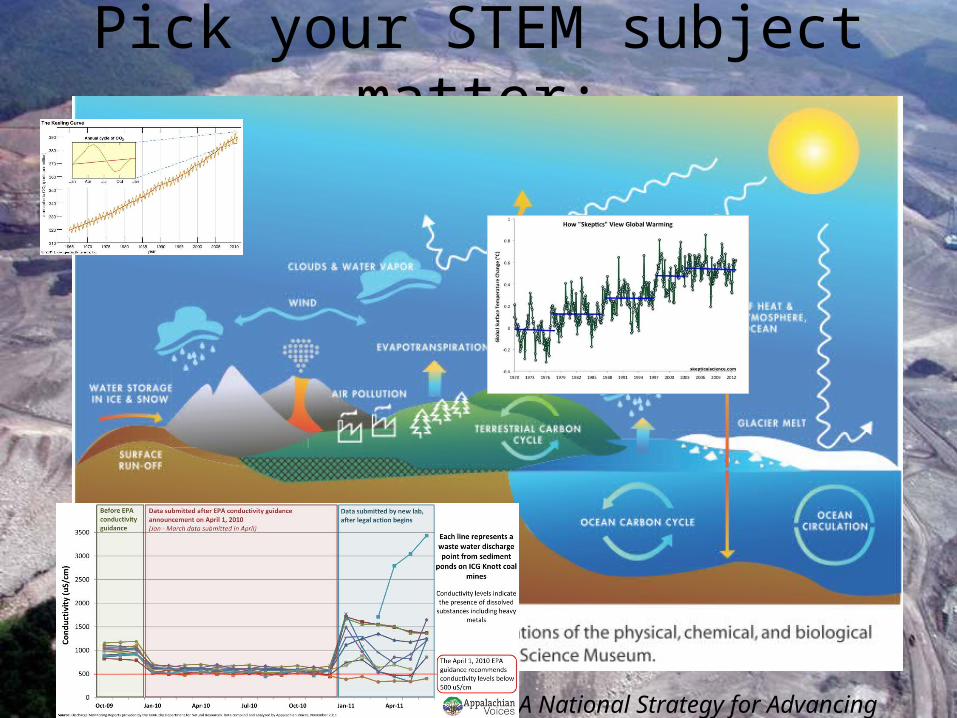
Variety: Pick your STEM subject matter
National Academy Press (2012): A National Strategy for Advancing Climate Modeling
Atmosphere
LithosphereHydrosphere
Cryosphere
Astronomy
Biosphere

Example (Math) Topic: Non-Linearity versus Linearity
And let’s focus on sea-level in this concrete example. There are, of course, many issues offering a variety of lines of attack from the GCD perspective. E.g. one could address:– Normal versus non-normal distributions– Regression modeling– Orthogonal functions and Fourier analysis– Correlation versus causation– …..
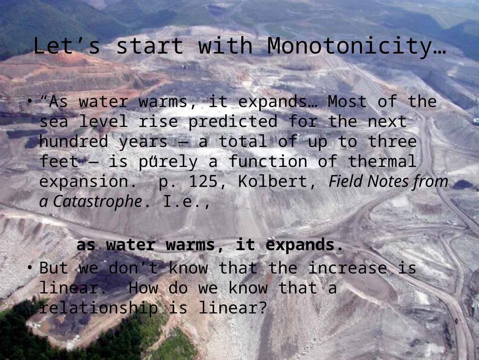
Let’s start with Monotonicity…
• “As water warms, it expands… Most of the sea level rise predicted for the next hundred years — a total of up to three feet — is purely a function of thermal expansion.” p. 125, Kolbert, Field Notes from a Catastrophe. I.e.,
as water warms, it expands.• But we don’t know that the increase is linear.
How do we know that a relationship is linear?

Linearity
• If you double x, does the change in y double? If so, y is an affine function of x, whose graph is linear. (If y itself doubles when x doubles, then y is truly linear.)
• So: if you double global output of CO2, does the warming double? Does ocean acidification double? Does twice as much Arctic ice melt? Do twice as many species go extinct?
• “[The WAIS]’s melting currently contributes 0.3 millimeters to sea level rise each year. This is second only to Greenland, whose contribution to sea level rise has been estimated as high as 0.7 mm per year.” West Antarctica warming more than expected (NCAR, 2012) A statement like this is an implicit declaration of linearity, and we find such statements (predictions) made all the time.

Most Phenomena are Non-Linear• An historical example (John Tyndall, 1861): “…
increasing the concentration of an absorbent gas does not always produce a proportional increase in heat uptake, because there is progressively less to be absorbed.” This explicitly denies linearity in a monotone relationship. In fact, linearity is generally rare in nature (but don’t tell our students!).
• Even monotonicity is violated frequently: for example, Paracelsus (the “father of toxicology”) said that everything is a poison in the wrong dose…. This asserts that positive inputs have U-shaped responses.

Mean Sea Level
20 years of linear growth…? Apparently: if we measure from any fixed point in time, e.g. if we double the time from 1993, then the change in mean sea level appears to double.
Looks like there’s a linear trend, with a dramatic downtrend in the last few years (followed by a surge to “catch up” – what’s up with that?).
Students need to realize that data – the dots – must be “connected” by the mathematician – and perhaps explained by the mathematician – or scientist – as well.
At times during the Cenozoic (~65 million years ago) the world was ice-free, and sea level was around 70 meters higher than today. “Sea level rise, despite its potential importance, is one of the least well understood impacts of human-made climate change.” Hansen, 2012. At this rate, it will take 22222 years to get to 70 meters again….

Or IS it linear? If we zoom out…
Two thousand years of sea-level rise estimates from two North Carolina salt marshes (Sand Point and Tump Point). Errors in the data are represented by parallelograms. The red [curve] is the best fit to the sea-level data. Green shapes indicate when significant changes occurred in the rate of sea-level rise. SOURCE: Kemp et al. (2011). From: Sea-Level Rise for the Coasts of California, Oregon, and Washington: Past, Present, and Future (National Research Council, 2012).

James Hansen Reviews Sea-Level
Update of Greenland Ice Sheet Mass Loss: Exponential? 12/26/2012:
“… the fundamental issue is linearity versus non-linearity.”
What about thatglacial contribution?
This graph of Greenland ice melt presents other issues which every student needs to address eventually, e.g. messy data (variability).
It also challenges students to think about which model is best – and perhaps even what model would be better!
Or at least the contribution from glaciers….

Pick your STEM subject matter:
National Academy Press (2012): A National Strategy for Advancing Climate Modeling
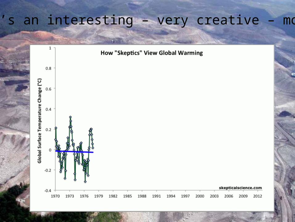
Here’s an interesting – very creative – model…

Pick your STEM subject matter:
National Academy Press (2012): A National Strategy for Advancing Climate Modeling

Favorite Example of Non-Linearity:The Keeling Data, Graphed
There is thetrend, and then there is the seasonal oscillation.
Each of these is a topic in its own right: non-linear versus linear growth, and periodicity.
Pick your STEM subject matter:
National Academy Press (2012): A National Strategy for Advancing Climate Modeling

ICG Pollution Reports Show Pattern of Deception
An example of a piece-wise defined function, with three clear reasons for the distinct pieces. This example provides a lot of grist for the function mill: variation (or lack thereof) can help determine that someone is faking it. [But why fake slightly above the legal limit?!]
(Thanks to Eric Chance and Appalachian Voices for the use of this example.)

Conclusions1. Data-based graphics are beautiful tools for
investigating and teaching elements and techniques of math and stats.
2. Topics can be motivated, embellished, or illustrated using these graphics.
3. Data is often available to do your own analysis – to create your own graphics and analyses.
4. GCD provides • variety,• accessibility, and• meaning and import.• Now for some action?

• General Resources:– Climate Change Indicators in the United States (EPA, 2012) (and graphics)– Climate Change: Evidence, Impacts, and Choices (National Research Council,
2012) (and graphics)• Additional Graphics resources
– Climate Graphics by Skeptical Science– UNEP Maps & Graphics Library– IPCC Fourth Assessment Report, Climate Change 2007 (AR4), Figures and Tables

Resource Greatest Hits• General Resources:
– Climate Change Indicators in the United States (EPA, 2012) (and graphics)– Climate Change: Evidence, Impacts, and Choices (National Research
Council, 2012) (and graphics)– Quantitative Environmental Learning Project (QELP) – e.g.
Keeling Data project
• Additional Graphics resources– Climate Graphics by Skeptical Science– UNEP Maps & Graphics Library– IPCC Fourth Assessment Report, Climate Change 2007 (AR4), Figures and
Tables
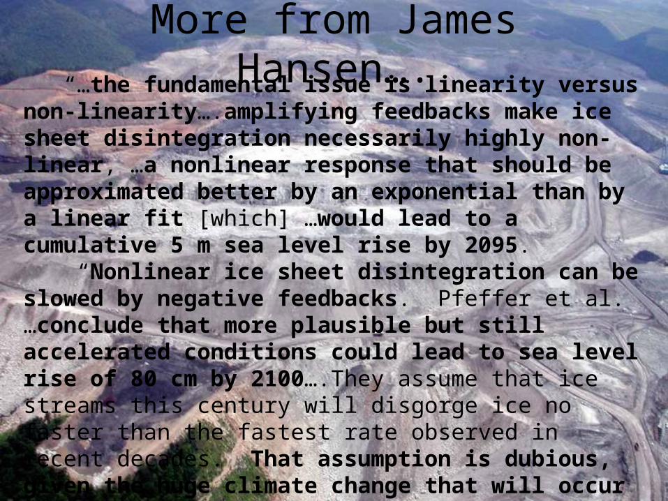
More from James Hansen…. “…the fundamental issue is linearity versus non-linearity….amplifying feedbacks make ice sheet disintegration necessarily highly non-linear, …a nonlinear response that should be approximated better by an exponential than by a linear fit [which] …would lead to a cumulative 5 m sea level rise by 2095. “Nonlinear ice sheet disintegration can be slowed by negative feedbacks. Pfeffer et al. …conclude that more plausible but still accelerated conditions could lead to sea level rise of 80 cm by 2100….They assume that ice streams this century will disgorge ice no faster than the fastest rate observed in recent decades. That assumption is dubious, given the huge climate change that will occur under BAU scenarios, which have a positive (warming) climate forcing that is increasing at a rate dwarfing any known natural forcing. BAU scenarios lead to CO2 levels higher than any since 32 My ago, when Antarctica glaciated.”


