Global Crude to Local Food: An Empirical Study of Global Oil Price Pass-through to Maize Prices in East Africa Brian M. Dillon a and Christopher B. Barrett b * December 2013 revised version Abstract: We study the transmission of global crude oil and maize prices to local maize prices across east Africa. Consistent with several recent papers, we do not find a significant causal relationship between oil and maize prices at the global market level. However, global oil prices do strongly affect maize prices at sub- national markets through their impacts on transport fuel prices. When we allow for the potential effects of local fuel prices on the price spread between maize markets, the average price elasticity of local maize with respect to global oil prices is 0.26. For 7 of the 17 markets in the study – and particularly for the 3 markets farthest from the coast – global oil prices have larger effects on local maize prices than do global maize prices. Furthermore, oil price shocks transmit much more rapidly throughout the region than do maize price shocks. This suggests that the short term effects of correlated commodity price increases on food prices in Africa may be driven more by rising transport costs than by the rising costs of food grains on global markets. Keywords: food prices; energy prices; price pass-through; African development; agricultural markets JEL codes: O13, Q11, F15 a Evans School of Public Affairs, University of Washington; [email protected]b Charles H. Dyson School of Applied Economics and Management, Department of Economics, and David R. Atkinson Center for a Sustainable Future, Cornell University; [email protected]* We thank Joanna Barrett and Shun Chonabayashi for research assistance, Chris Adam, Heather Anderson, Channing Arndt, Marc Bellemare, Harry de Gorter, Oliver Gao, Miguel Gómez, Yossie Hollander, Wenjing Hu, David Lee, Matt Nimmo-Greenwood, Per Pinstrup-Andersen, Tanvi Rao, Stephan von Cramon-Taubadel and seminar participants at Cornell, Melbourne, Monash and Sydney universities for helpful comments on earlier drafts, and the Bill and Melinda Gates Foundation for financial support of this project. Assistance in gathering data from government sources was provided by Mujo Moyo in Tanzania, Bjorn Van Campenhout, Todd Benson, and Andrew Mutyaba in Uganda, Pasquel Gichohi in Kenya, and Bart Minten, Guush Tesfay, and Temesgen Mulugeta in Ethiopia. This project was partly undertaken through a collaborative arrangement with the Tanzania office of the International Growth Center. Barrett thanks Monash University and the University of Melbourne for their hospitality while he worked on this paper, and Dillon thanks the Harvard Kennedy School for support through the Sustainability Science program. Any errors are the authors’ alone.
Transcript
Global Crude to Local Food:
An Empirical Study of Global Oil Price Pass-through
to Maize Prices in East Africa
Brian M. Dillona and Christopher B. Barrettb *
December 2013 revised version
Abstract:
We study the transmission of global crude oil and maize prices to local maize prices across east Africa.
Consistent with several recent papers, we do not find a significant causal relationship between oil and
maize prices at the global market level. However, global oil prices do strongly affect maize prices at sub-
national markets through their impacts on transport fuel prices. When we allow for the potential effects of
local fuel prices on the price spread between maize markets, the average price elasticity of local maize
with respect to global oil prices is 0.26. For 7 of the 17 markets in the study – and particularly for the 3
markets farthest from the coast – global oil prices have larger effects on local maize prices than do global
maize prices. Furthermore, oil price shocks transmit much more rapidly throughout the region than do
maize price shocks. This suggests that the short term effects of correlated commodity price increases on
food prices in Africa may be driven more by rising transport costs than by the rising costs of food grains
a Evans School of Public Affairs, University of Washington; [email protected] b Charles H. Dyson School of Applied Economics and Management, Department of Economics, and
David R. Atkinson Center for a Sustainable Future, Cornell University; [email protected]
* We thank Joanna Barrett and Shun Chonabayashi for research assistance, Chris Adam, Heather Anderson,
Channing Arndt, Marc Bellemare, Harry de Gorter, Oliver Gao, Miguel Gómez, Yossie Hollander, Wenjing Hu,
David Lee, Matt Nimmo-Greenwood, Per Pinstrup-Andersen, Tanvi Rao, Stephan von Cramon-Taubadel and
seminar participants at Cornell, Melbourne, Monash and Sydney universities for helpful comments on earlier drafts,
and the Bill and Melinda Gates Foundation for financial support of this project. Assistance in gathering data from
government sources was provided by Mujo Moyo in Tanzania, Bjorn Van Campenhout, Todd Benson, and Andrew
Mutyaba in Uganda, Pasquel Gichohi in Kenya, and Bart Minten, Guush Tesfay, and Temesgen Mulugeta in
Ethiopia. This project was partly undertaken through a collaborative arrangement with the Tanzania office of the
International Growth Center. Barrett thanks Monash University and the University of Melbourne for their hospitality
while he worked on this paper, and Dillon thanks the Harvard Kennedy School for support through the
Sustainability Science program. Any errors are the authors’ alone.
1
1. Introduction
The global food price crises of 2008 and 2011 drew widespread attention to the effects of commodity
price shocks on poverty and food security in the developing world. In the ensuing debate over the causes
of these price spikes, one prominent thread emphasizes the role of energy costs, particularly the price of
oil (Abbott et al. 2008, Headey and Fan 2008, Krugman 2008, Mitchell 2008, Rosegrant et al. 2008,
Baffes and Dennis 2013). Yet there is a notable absence of careful empirical analysis of the links between
food prices and energy prices at the level where food prices most affect the poor, i.e., in markets within
developing countries. Do global crude oil price shocks significantly affect local food prices, particularly
in countries with high levels of subsistence food production? If so, how much, and by what mechanisms?
This paper tackles those questions, focusing on maize markets in the four major east African
economies: Ethiopia, Kenya, Tanzania and Uganda. These markets are ideal for studying the food-energy
link in developing economies. Maize is the main input to global biofuels production due to the reliance of
the US ethanol industry on corn. Maize is the primary staple food in east Africa, serving as both the
greatest source of calories and a key income generator for farmers. And the region is distant from major
maize exporters and burdened with poor transport infrastructure, so that variable transport costs are
potentially relevant.
Oil prices can affect maize prices through three main channels. First, higher oil prices can
increase the cost of farm inputs such as inorganic fertilizer (which is made from natural gas) and fuel for
tractors or pumps. Second, higher global oil prices can stimulate market demand for corn to convert into
ethanol, thereby driving up maize prices on the global market, which transmit to local markets through
trade linkages. Third, oil price increases can drive up transport costs, which in turn affect the prices of all
traded commodities, food grains included.
The first channel is of second-order concern in the study countries, all of which are well-
integrated with world maize markets and act as pure price-takers on world maize markets. For these
economies, changes in production costs affect profits and output levels, but not long-run equilibrium
prices. Any direct effects of higher production costs will be captured by changes in global market maize
prices, which we observe and include in the analysis.1
The second channel rests on the premise that biofuel production creates a structural link between
oil prices and maize prices. This topic has received substantial attention since the passage of the ethanol
1 Farmer expenditure on fuel for tractors or irrigation pumps is zero for the vast majority of farmers in east Africa
(and total expenditure on these inputs is negligible). Kenya is the only study country in which fertilizer application
was commonplace during the study period. In Appendix C we show that, as expected, maize prices in Kenya are not
responsive to changes in the price of fertilizer. In the same section we also verify that after conditioning on global
market prices of maize and oil, global fertilizer prices are not an important determinant of domestic prices of maize
and fuel in all of the study countries.
2
mandate in the US Energy Policy Act of 2005 (Krugman 2008, Mitchell 2008, de Gorter et al. 2013).
However, the recent literature finds little empirical support for the hypothesis that oil price changes
transmit strongly to maize prices on global markets (e.g., Zhang et al. 2007, 2009, 2010, Gilbert 2010,
Serra et al. 2011, Enders and Holt 2012, Zilberman et al. 2013). We estimate a number of models relating
oil and maize prices on global markets, and likewise find no evidence of a systematic, causal link. We
therefore do not emphasize this channel. However, in interpreting results we do consider the case of
correlated increases in global oil and maize prices. In this sense our approach is conservative, because any
undetected links through biofuels markets would only amplify the effects that we find.
We focus on the third channel, the link through transport costs. Transport costs loom large in
African markets, because of the low value-to-weight ratio of grains, long distances between population
centers, and rudimentary transport infrastructure dependent primarily on trucks (lorries). Even though
subsistence food production is still widespread in the region, significant volumes of maize are traded
across space, and even across borders, in each of the study countries. The food supply to urban consumers
relies heavily on lorry-based grain shipments from the domestic breadbasket regions and from
international ports of entry. As we show, global oil prices exert considerable influence on sub-national
maize market prices through their effects on transport fuel prices.
Using a newly assembled data set of monthly, average maize prices and monthly, average petrol
prices (at the pump) from 17 sub-national markets for the period 2000-2012, we estimate the pass-through
effects on local maize prices of changes in the world market prices of oil and maize. Our empirical
approach involves stepwise estimation of error correction models. First, we estimate the impact of global
oil and global maize price changes on petrol and maize prices in the port-of-entry (POE) markets for the
four study countries. In this step we allow changes in global oil prices to impact the price margin between
POE maize and global maize. Next, we estimate the equilibrium pass-through rates of petrol prices from
the POE markets to other sub-national markets, to model changes in local transport costs. Finally, we
estimate the equilibrium pass-through rates of maize prices from the POE markets to other sub-national
markets, allowing changes in local petrol prices to directly impact the maize price spread. Following
Borenstein et al. (1997), in all steps we allow for the possibility of asymmetric adjustment to price
increases and decreases.
This empirical strategy rests on four key identifying assumptions, discussed in detail in Section 3.
Three of these are rather innocuous: first, that study countries are price takers on global markets; second,
which follows logically, that port-of-entry prices are weakly exogenous to interior market prices; and
third, that domestic fuel prices are weakly exogenous to domestic maize prices. The fourth and most
tenuous identifying assumption is that exchange rate changes are at least weakly exogenous to changes in
the global prices of oil and maize. While we believe this to be a restrictive (but necessary) assumption in
3
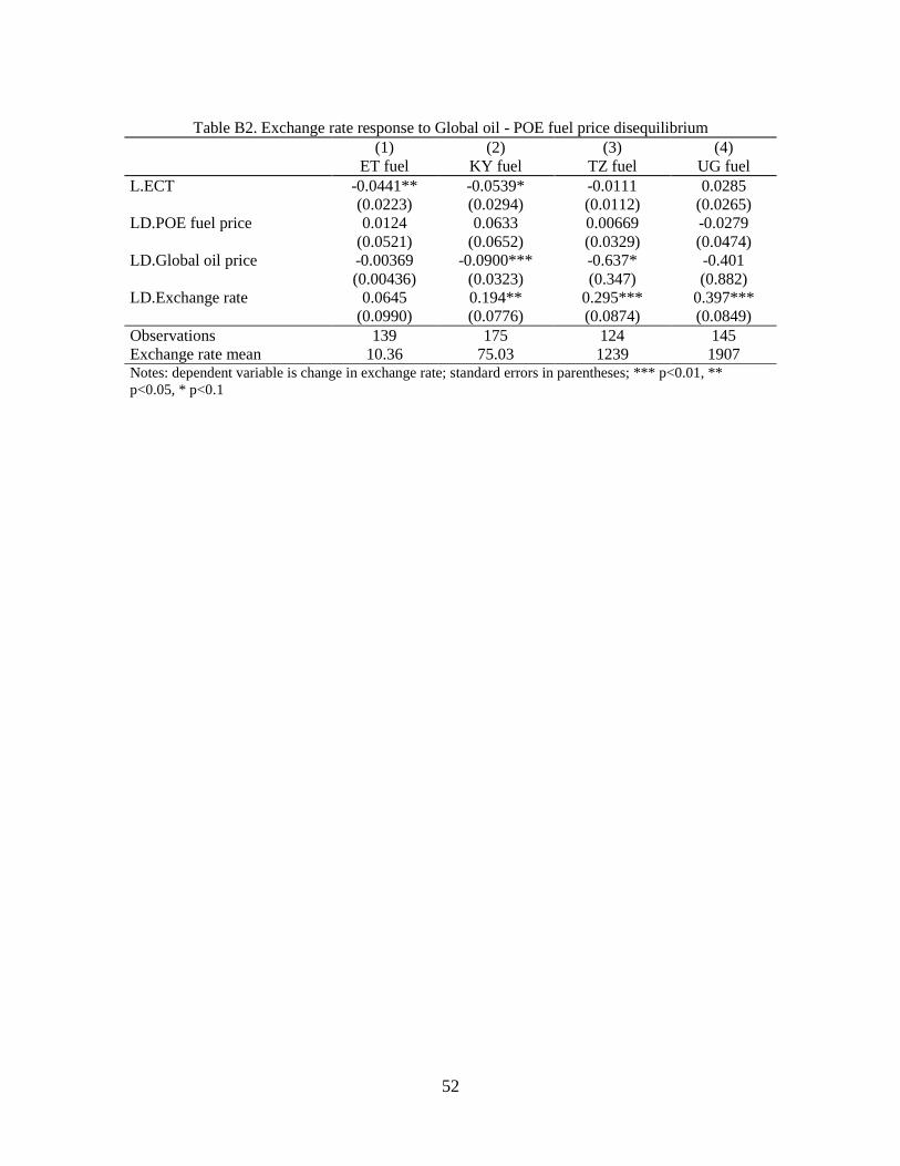
the long run, in Appendix B we show that there is evidence in support of exchange rate exogeneity in our
data.
We have three main results. First, we find an important role for global crude oil prices in
determining maize prices in local markets within east Africa. Across the 17 markets in our study, a 1%
increase in global oil prices is associated with an average long run maize price increase of 0.26%, even in
the absence of changes in global maize prices or in the exchange rate. This finding is remarkably stable
across study markets; all but 2 of the 17 estimated global-to-local oil price pass-through rates lies in the
range 0.10-0.41%. In comparison, a 1% rise in global maize prices, absent a corresponding change in oil
prices or exchange rates, leads to a 0.42% average local maize price increase, with considerably more
dispersion among markets. When global oil and maize prices simultaneously increase by 1%, the average
increase in local maize prices is 0.68%. Any remaining maize price adjustments operate via the exchange
rate (more on that in Sections 3 and 5). These estimated rates of price transmission are substantially
greater than those in much of the current literature, which are likely biased downwards by the omission of
transport costs (Benson et al. 2008, Abbott and Borot de Battisti 2011, Baltzer 2013).
Second, in the three markets that are farthest from an ocean port (Gulu and Mbarara, Uganda, and
Kigoma, Tanzania), as well as in all of the Kenya markets, the elasticities of local maize prices with
respect to global oil prices are equal to or greater than those with respect to global maize prices. In these
land-locked areas, variable transport costs have a large and often overlooked effect on food prices, and
therefore on food security. Indeed, across the sample we find that the estimated elasticity of local maize
prices with respect to global oil prices is increasing in distance from the port-of-entry.
Third, because we observe local market prices for both food and fuel, we are also able to estimate
the speed with which global price changes transmit to local grain prices. We find that oil price shocks
transmit much more rapidly to local maize prices than do global maize price shocks. In three-quarters of
the markets, increases in global oil prices transmit more than twice as rapidly as global maize price
increases. This is likely because all liquid fuel consumed in the region is imported, and trade is the only
way to clear the market. Maize, in contrast, is produced by tens of millions of spatially dispersed farmers,
allowing for local supply adjustments and consumption out of stocks that dampen the speed of price
transmission. Also, food prices are a political flashpoint. Ad hoc policy responses to mitigate food price
shocks, such as export bans or releases of reserves, are not uncommon (Ivanic et al. 2012, Barrett 2013,
Pinstrup-Andersen 2013). An important implication of this speed-of-adjustment finding is that when oil
prices and maize prices co-move on global markets, as they often do, the immediate effect on food prices
may be due as much or more to changes in transport costs than to changes in the global prices of the
grains. To the extent that policymakers ignore the fuel channel and attempt to mitigate food price spikes
4
by intervening exclusively in grain markets, policy responses may not achieve the desired price
stabilization effects.
There is a large literature in economic history and development economics that deals with
transport costs, but the emphasis tends to be on the fixed cost components of transport – roads, railways,
etc. – and their relation to economic outcomes.2 Here, our interest is the link between variable transport
costs and the price of food in low income countries. To our knowledge this is the first paper to make use
of local transport fuel prices in a study of food price determination in the developing world. While the
fuel-food price connection is a frequent topic in the popular press, there is little rigorous research on this
topic. This is likely due to the scant availability of data on variable transport costs (World Bank, 2009, p.
175), which we assembled from a wide range of government sources, as described below.
This paper also speaks to broader economic questions of time-varying market frictions and
asymmetric price adjustment (Engel and Rogers 1996, Borenstein et al. 1997, Peltzman 2000, Evans
2003, Anderson and van Wincoop 2004). Where much of the existing literature struggles to identify the
source(s) of frictions that give rise to incomplete, slow, or asymmetric price pass-through, for example in
financial markets (Constantinides 1986, Anderson 1997, Michael et al. 1997), here the frictions arise
naturally from observable variation in transport costs. The fact that oil prices exert a substantial influence
on grain prices purely through transport costs underscores the important role that such frictions can play
in market price determination.
Finally, these questions hearken back to an earlier literature in which economists worried about
commodity price dynamics and global-to-local price transmission because of their impacts on developing
countries, especially in Africa (Ardeni and Wright 1992, Deaton and Laroque 1992, 1996, Deaton 1999).
As Deaton (1999, p.24) laments, speaking of commodity exports, “the understanding of commodity prices
and the ability to forecast them remains seriously inadequate. Without such understanding, it is difficult to
construct good policy rules.” The same concern applies today. In the absence of careful empirical analysis
of commodity price behavior, even thoughtful commentators may misunderstand the drivers of observed
price patterns, with important implications for policy.
The rest of the paper proceeds as follows. In Section 2 we describe the data and the setting. In
Section 3 we outline the empirical framework. Section 4 contains the empirical results. Section 5
discusses findings and presents the cumulative pass-through elasticities. Section 6 concludes.
2. Data and Setting
2 See, among numerous others: Fogel 1964, Chandra and Thompson 2000, Jacoby 2000, Limão and Venables 2001,
Baum-Snow 2007, Jacoby and Minten 2009, Atack et al. 2010, Buys et al. 2010, Bell 2012, Storeygard 2012,
Donaldson forthcoming.
5
Background and setting
According to the 2009 FAO Food Balance Sheet data, maize is the largest source of calories in Ethiopia,
Kenya, and Tanzania. In 2009 the average Ethiopian consumed 418 kcal/day of maize (accounting for
20% of total dietary energy intake), the average Kenyan consumed 672 kcal/day (32%), and the average
third in importance behind plantains and cassava but still critical to food security. Maize consumption in
Uganda varies regionally, with greater consumption in the north and east than in the southwest.
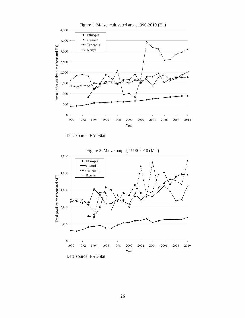
Table 1 shows the allocation of land to maize and categories of other crops over the period 2007-
2010. In Kenya and Tanzania, more land is allocated to maize than to the total of all crops in any other
category. In all four countries the land area of maize cultivation is greater than that of any other single
crop (not shown).3 In Figures 1 and 2 we plot the time path of annual cultivated maize acreage and total
annual maize output, respectively, for the four study countries. In Ethiopia, Kenya, and Uganda, both
series show upward trends over the study period (2000-2012). In Tanzania, however, the data show a near
doubling of maize acreage from the 1990s to the 2000s, with a sharp change in maize output in 2002. This
is likely due to systematic measurement error that was corrected with the 2002 agricultural census.4
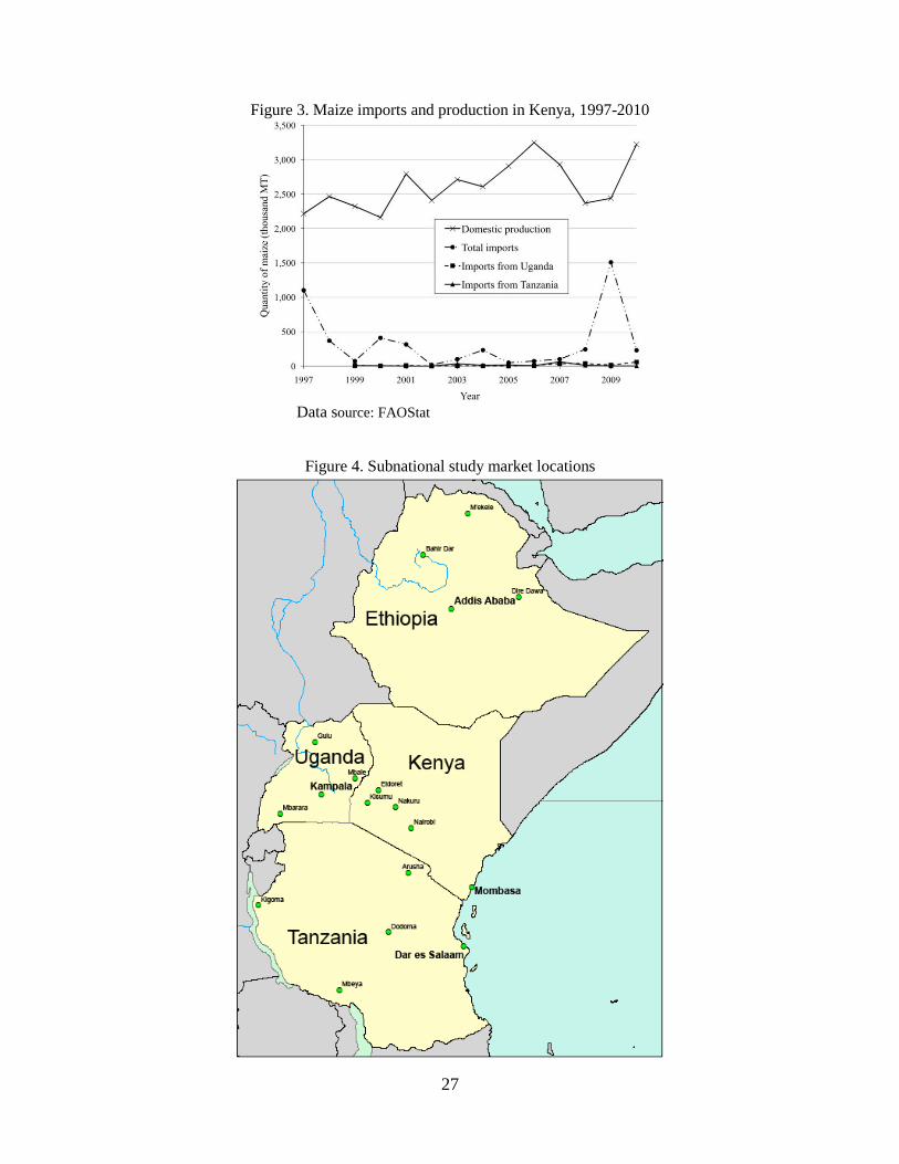
In Table 2 we report annual maize net import (imports – exports) statistics for the four study
countries over the period 2000-2010. All four countries are engaged in the international maize trade,
although volumes of both exports and imports are low relative to consumption. Only in Kenya does
international trade account for a significant portion of traded maize, with substantial variation between
years. In Figure 3, which shows maize production and imports in Kenya for the period 1997-2010, it is
only in 1997 and 2009 that net maize imports account for more than 20% of consumption.
Since the 1990s, in lockstep with the general shift in the developing world away from planning
and toward market determination of prices and trade flows, governments in the four study countries have
largely withdrawn from direct participation in the production, distribution, or pricing of food and fuel.
The exception is the price of fuel in Ethiopia, which is set for each major market by the Ministry of Trade
and Industry. Other relevant policies, such as tariffs, procurement auctions, maintenance of strategic grain
reserves, and occassional ad hoc export bans, are discussed in Appendix A.
Data sources and descriptive statistics
Figure 4 shows the location of the 17 markets for which we could match fuel and maize price series. All
are urban areas, but of varying size and remoteness from global markets. The POE markets – Mombasa,
Kenya; Dar es Salaam, Tanzania; Kampala, Uganda; and Addis Ababa, Ethiopia – are indicated with a
3 See FAOstat for details by crop. Rashid (2010) gives a detailed descriptive analysis for Ethiopia. 4 While the FAO data are the best available, we suggest that the output and acreage numbers be read with caution.
Recent work on data quality in African agriculture statistics shows significant measurement error (Jerven 2013).
6
larger font size. We use monthly average prices for all data series because higher frequency data were not
available for sub-national petrol and maize markets. We focus on the period 2000-2012, with slight
variation in the coverage period due to data limitations.
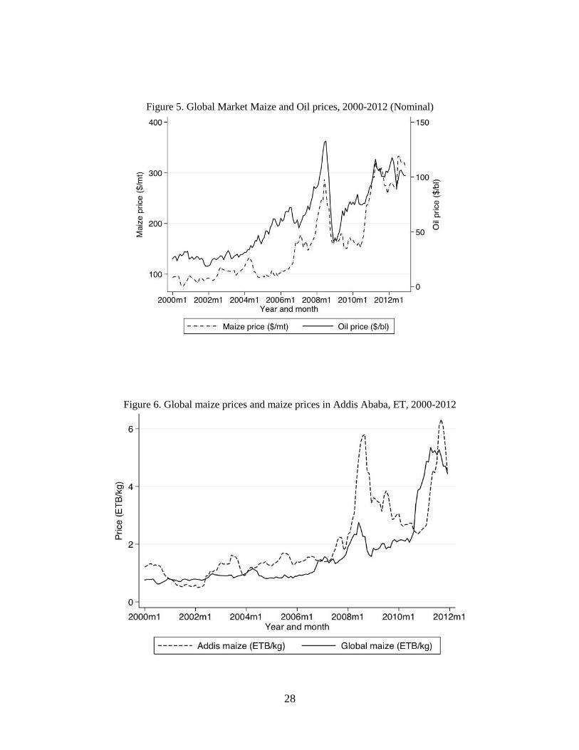
Global market price series are from the World Bank Global Economic Monitor (GEM)
commodity price database. Crude oil prices are expressed in nominal USD per barrel, and are the equally
weighted average of Brent, Dubai, and West Texas Intermediate spot prices. Maize prices are nominal
USD per metric ton for number 2 yellow maize, f.o.b. at US Gulf ports. In Figure 5 we plot the global
price series over the study period. The series co-move somewhat, although no obvious causal relationship
presents itself. The correlation coefficient between the nominal price series is 0.83. After deflating to
2005 prices using the world CPI measure from the IMF IFS data, the correlation coefficient is 0.45.
In regressions with both global and national prices, we use the monthly CPI and $US exchange
rate for each study country. These data are from the IMF International Financial Statistics database.
Wholesale prices of white maize for markets in Kenya are from the USAID-funded Famine Early
Warning System (FEWS). Average wholesale maize prices for Tanzania were provided by the Ministry of
Agriculture, via the International Growth Center (IGC) office in Dar es Salaam. Wholesale maize prices
for Ethiopia markets are from the website of the Ethiopia Grain Trade Enterprise (EGTE). Retail white
maize prices for Uganda markets are from the Regional Agricultural Trade Intelligence Network
(RATIN) of the East Africa Grain Council (wholesale prices were not available).5
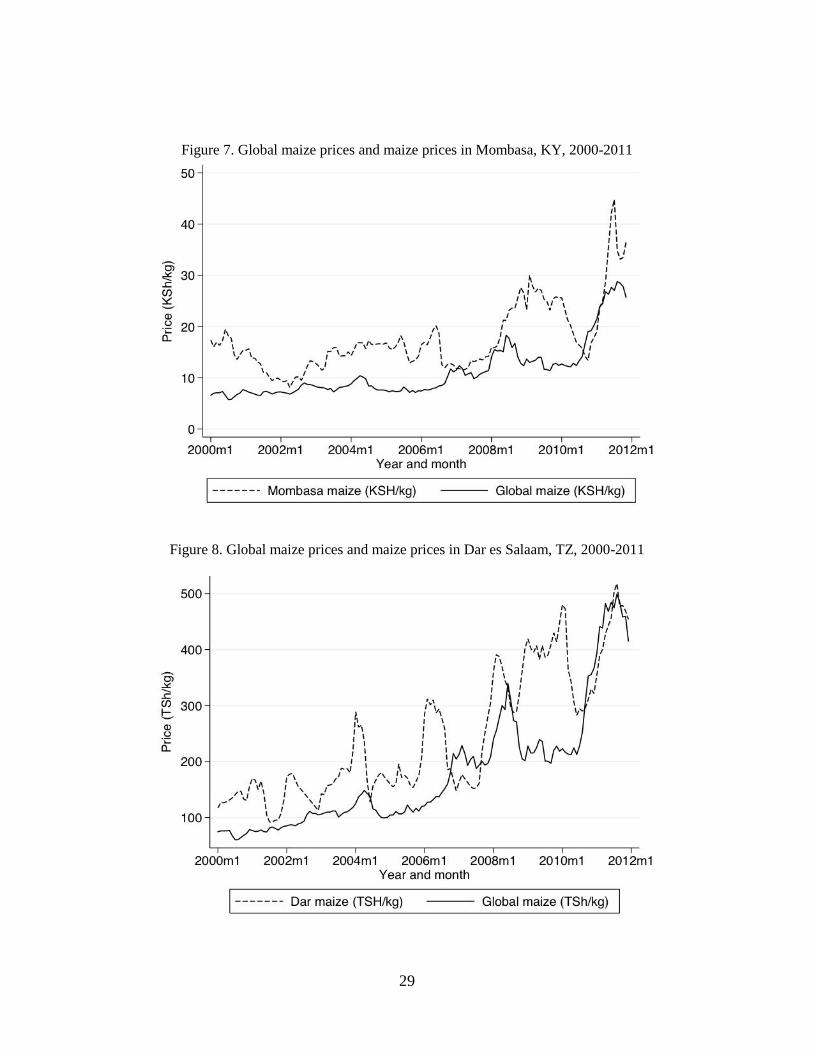
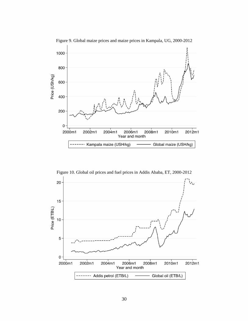
In Figures 6-9 we plot the POE maize prices for each country against global maize prices.6 In
each figure, global prices in month t are converted to local, nominal currency units using the exchange
rate in month t. While intra-annual seasonality related to the harvest cycle is clearly visible in each graph,
the long-run trajectory of prices in each market tracks the shifts in global prices.
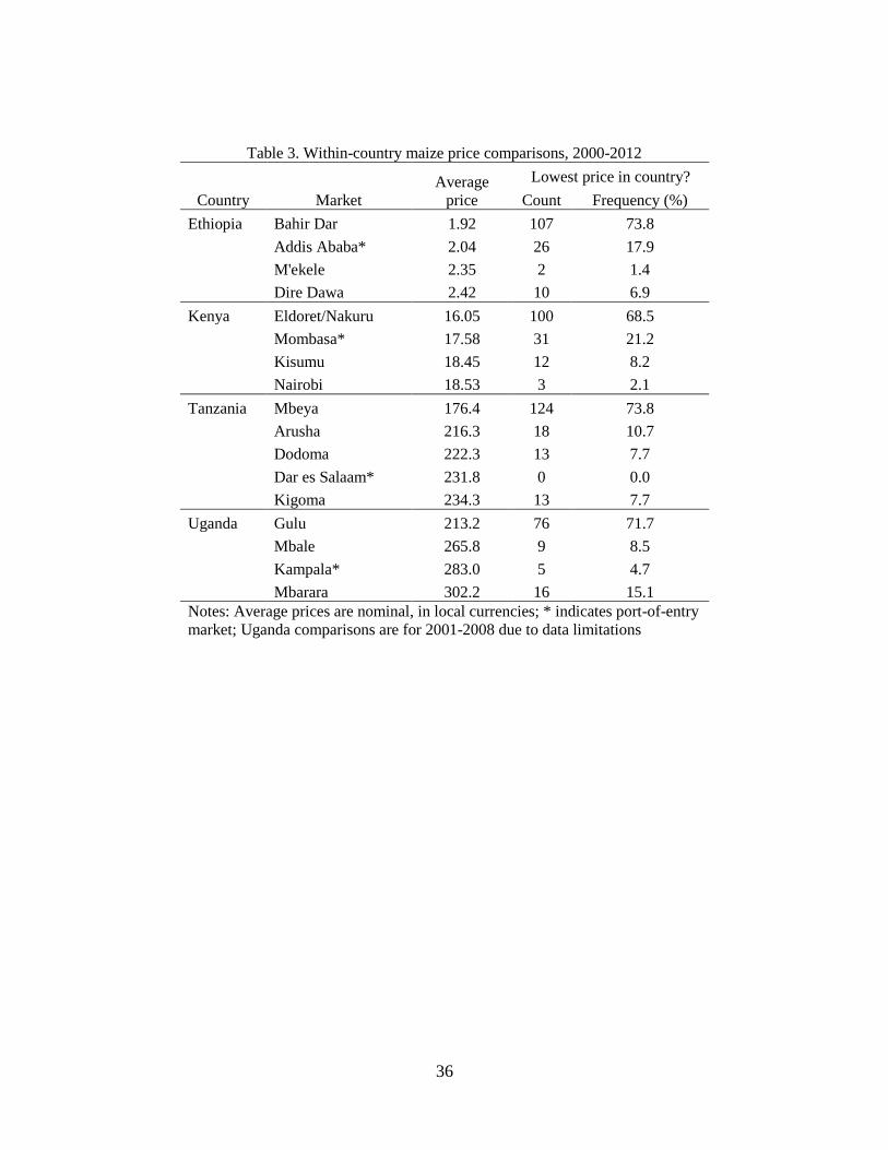
Table 3 shows the average price of maize at study markets, along with the number and percentage
of study months in which the price in each market was the lowest in the country. Not surprisingly, the
lowest average prices are in the trading centers near the maize breadbasket regions (Bahir Dar, Ethiopia;
Eldoret/Nakuru, Kenya; Mbeya, Tanzania; Gulu, Uganda). Perhaps the only surprise in Table 3 is that
maize prices in Mombasa, Kenya, tend to be lower than those in Kisumu and Nairobi. Very little maize is
grown in the coastal areas around Mombasa. This likely reflects the fact that the coastal region is
primarily served by imports rather than by trade of domestically produced maize, so that the net maize 5 Price series for Uganda are less complete than those for other markets, with very few observations after 2008 and
spells of missing data in other years. However, there are alternative sources of prices for Uganda that overlap the
RATIN price series in some periods, such as FEWS, Uganda FoodNet, and the FAO. To accommodate missing
values in the Uganda RATIN series, we predict prices using least squares estimates based on regressions of RATIN
prices on these other price series, and on RATIN prices in non-study markets. Details available upon request. 6 Note that farmers in study countries typically grow white maize, but we have global prices for yellow maize. We
believe this to be of little consequence: data is only maintained for one type of maize because the two are broadly
considered substitutes.
7
transport costs to Mombasa are lower for international exporters than those to more centrally located
cities.
For fuel prices we use petrol prices at the pump rather than the arguably more relevant diesel
prices, because of data availability.7 The market-specific mandated prices in Ethiopia, along with the
exact dates of all price changes, were provided by the Ministry of Trade and Industry. Petrol prices in
Uganda are monthly averages provided by the Consumer Price Index division of the Bureau of Statistics.
Monthly average retail prices for markets in Kenya were provided by the Kenya National Bureau of
Statistics. 8 Monthly average retail petrol prices for markets in Tanzania were provided by the Bank of
Tanzania and IGC.
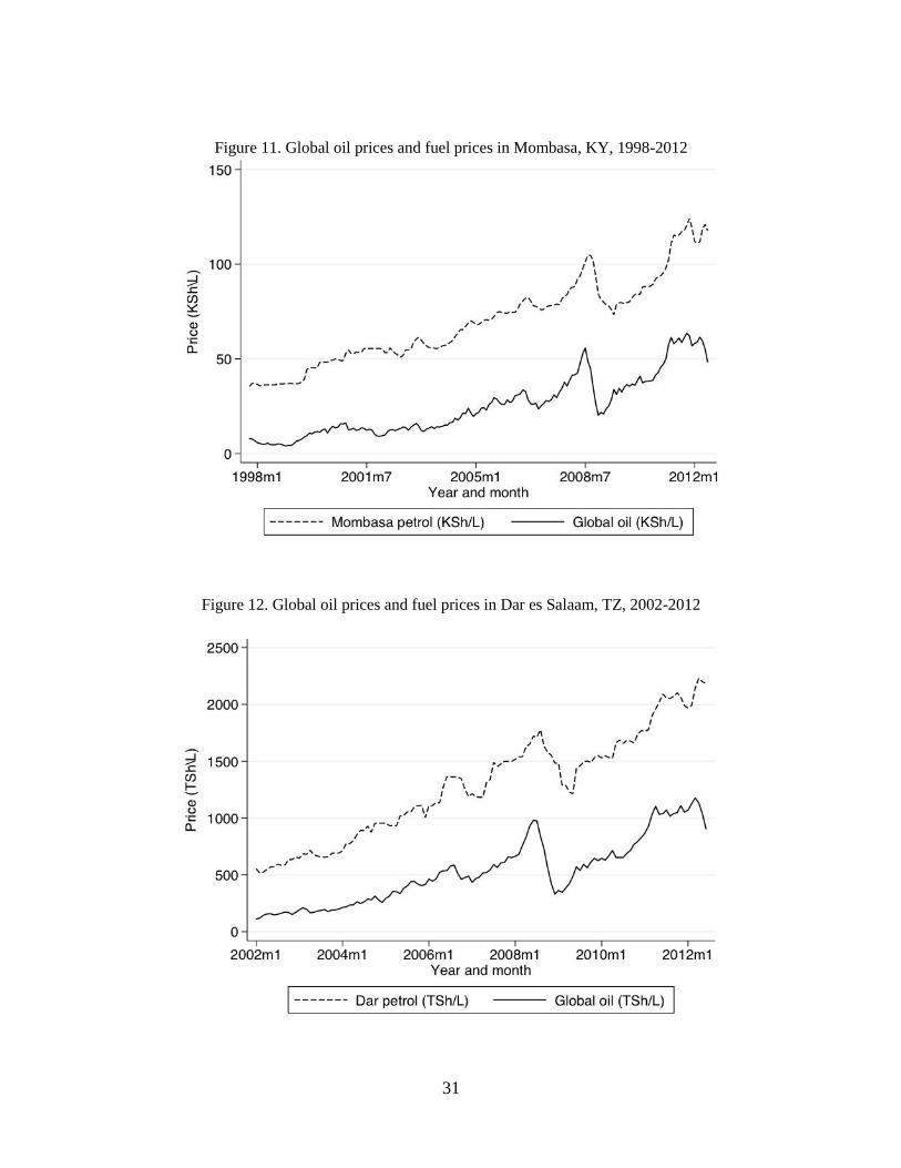
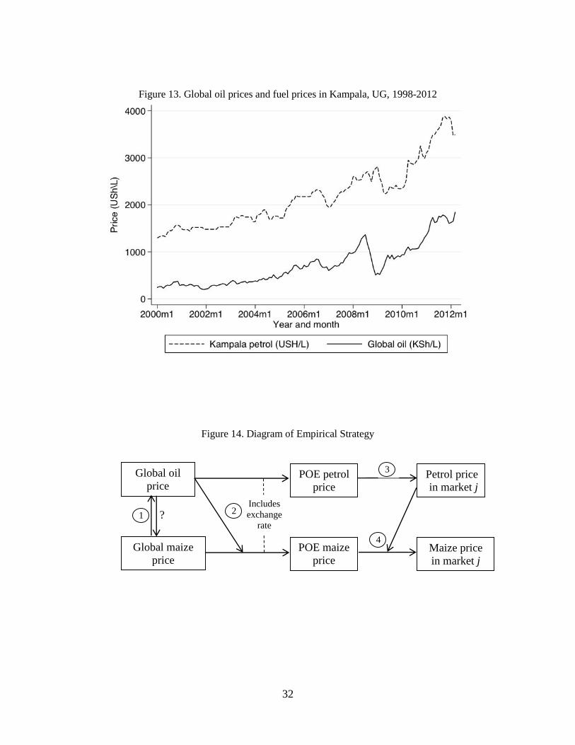
Figures 10-13 show the time path of POE fuel prices along with global oil prices. It is clear that
each POE-global pair closely co-move, with changes in the POE price tending to lag global price changes.
Infrequent updating of the Addis Ababa petrol price, a consequence of government-mandated pricing, is
clear in Figure 10.
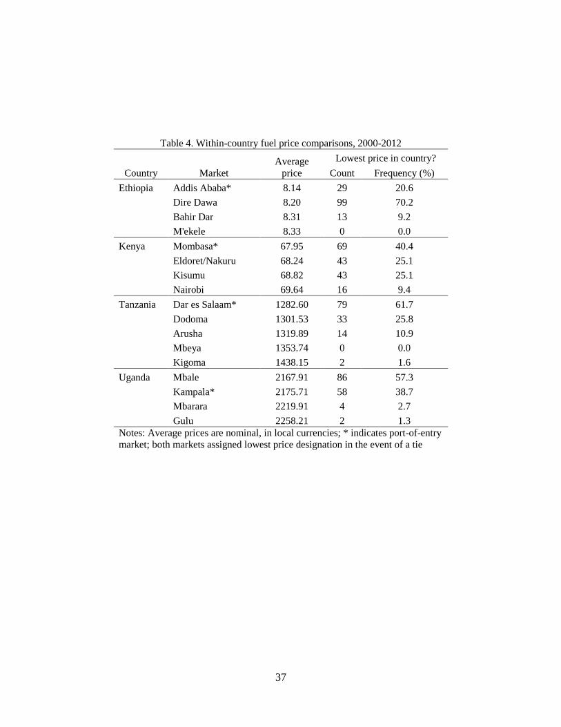
Table 4 shows the average price of fuel at sub-national markets in the sample data, along with the
number and percentage of study months in which the price in each market was the lowest in the country.
As expected for an imported good, fuel prices in the POE market are the lowest on average in Ethiopia,
Kenya, and Tanzania. In Uganda, retail fuel prices in the Kampala are slightly higher on average than in
Mbale, indicating that some fuel imports from Kenya may be diverted directly to Mbale (which is near the
border) without first passing through Kampala.
3. Empirical Approach
All of the price series in this paper are I(1).9 Our empirical strategy involves stepwise estimation of error
correction models treating the larger market price (global price in one step, POE price in the next) as
weakly exogenous to the smaller market price. Figure 14 summarizes the approach. We begin by
estimating the relationship between the global prices of oil and maize (step 1). We then estimate the
impact of changes in global market prices of each commodity on the POE prices in each country,
separately, treating the global price as weakly exogenous (step 2). Changes in global oil prices are
included in the POE maize equations in order to allow for variable transport cost margins at the border.
We then estimate the link between POE petrol prices and petrol prices in geographically dispersed sub-
7 This is of minimal concern, as the prices are highly correlated in those markets for which we have both. 8 In one location we have to merge series from proximate towns. We could assemble fuel price data from Nakuru but
not from Eldoret, while the maize price series from Eldoret was complete and that from Nakuru truncated. Since
these are quite proximate and the two main urban concentrations of Rift Valley Province in Kenya, we merge them
into a synthetic series, using Eldoret’s maize prices and Nakuru’s fuel prices. 9 Results, based on the modified Dickey-Fuller test (Elliott et al. 1996) and the Phillips and Perron (1988) test, are
available upon request.
8
national markets (step 3). Finally, we estimate the pass-through rates of maize prices from the POE
markets to other sub-national maize markets, allowing changes in local fuel prices to impact the maize
price spread (step 4).10
This approach rests on four key identifying assumptions:
Assumption 1. Each country is a price taker on global markets for both maize and oil, so that the global
market price is at least weakly exogenous to POE prices. This is an innocuous assumption given each
country’s small share of global trade in these two commodities.
Assumption 2. There is no feedback from maize prices to fuel prices within study countries, rendering
petrol prices weakly exogenous to maize prices intra-nationally. This is also a mild assumption given the
absence of any significant biofuel production and the small share of maize in gross freight haulage within
the region.
Assumption 3. Global prices are transmitted to local markets via the POE, so that the POE prices are
weakly exogenous to interior market prices. This assumption follows from assumption 1 and the
continuity of international trade in both commodities in almost all months. As a consequence, any
disequilibrium between prices at the POE and those in other market j is resolved through adjustment in j.
While this may be a simplification in the very short run, it is surely a benign assumption in the medium
and long term, because trade with international markets, and therefore the price-setting mechanism, is
mediated primarily through the POE.
Assumption 4. The exchange rate is weakly exogenous to changes in oil and maize prices over the study
period. If there is an identification challenge in the paper, it relates to this fourth assumption. A full
model of exchange rate determination would involve numerous other variables, and would take us well
beyond the scope of this paper. However, we include monthly exchange rates in the long run equations of
all models linking global prices to domestic prices, and in Appendix B we show that in general, exchange
rates do not respond to maize or oil market disequilibrium. Nevertheless, over a long enough time
horizon, exchange rates are likely endogenous to commodity price changes. In the interpretation of
results, we accommodate this possibility by separately assuming zero and complete exchange rate
adjustment to changes in commodity prices, which gives bounds on cumulative pass-through elasticities.
10 Enders (2010) lays out the general approach to VAR and error correction models that we use in this paper.
9
Finally, in regard to the multi-step estimation procedure, we believe it is important to estimate the POE-
global price link in a first stage because this allows us to measure the effects of country-specific tariffs
and import policies. Then, equations linking the POE price to each sub-national market allow for distance,
infrastructural differences, and possible local market effects to differentially affect the rate at which
global prices transmit within national markets.11,12
Step 1. Global Oil - Global Maize Price Linkages
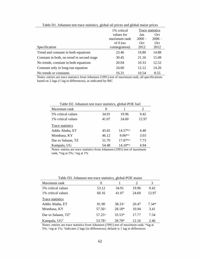
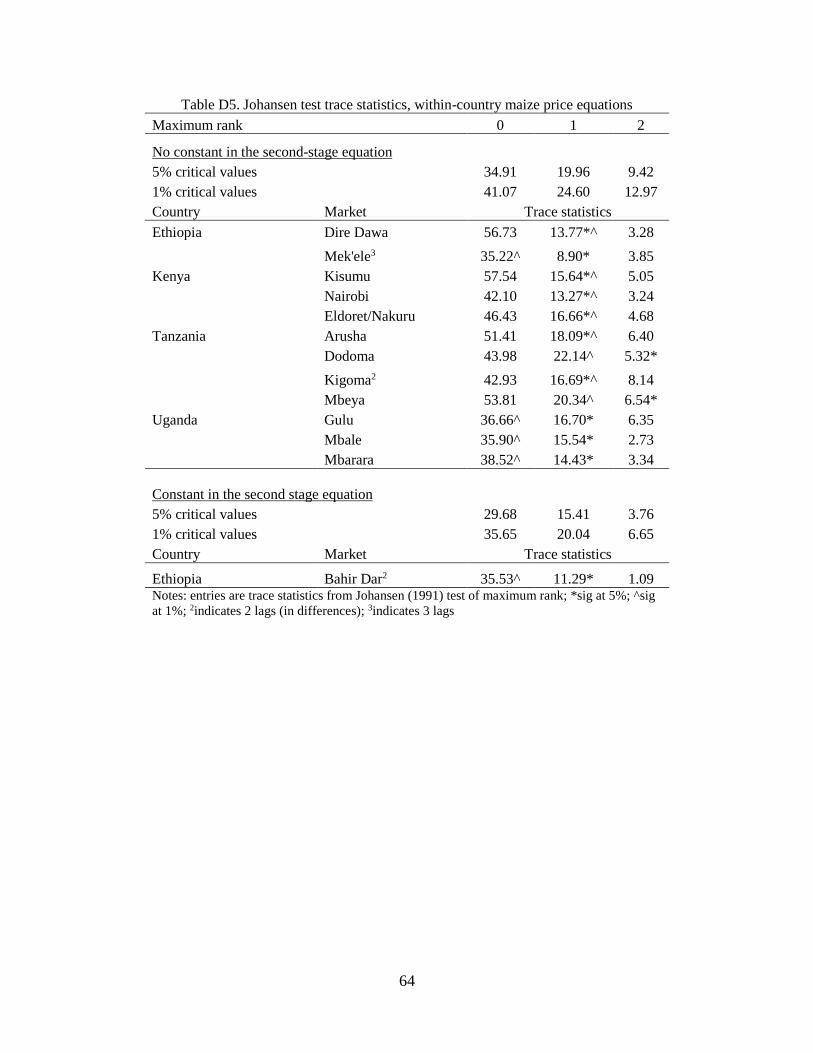
Rank tests for the maximum number of cointegrating vectors (Johansen 1991, 1995) indicate that the
global price series are not cointegrated at conventional levels of significance (Appendix D has results of
all cointegration tests). This result does not change if we include a trend or suppress the constant in the
cointegrating equation. Using different, US price series, Zhang et al. (2009) and Serra et al. (2011)
similarly find no evidence of cointegration between monthly crude oil and corn price series. Zhang et al.
(2010) find precisely the same result using the same data series, but with somewhat earlier dates.
This finding does not account for the ethanol mandate that took effect in October 2006, under the
United States Energy Policy Act of 2005, which may have fundamentally changed the relationship
between fossil fuel prices and maize prices (de Gorter et al. 2013). However, Johansen tests on data from
October 2006 onwards still do not show evidence of cointegration between the series. This result is
consistent across specifications (including trends, suppressing constants), and holds for both nominal and
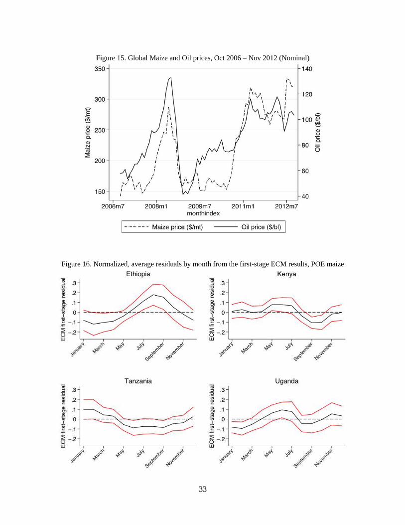
real prices (not shown). The lack of cointegration between these series is perhaps evident in Figure 15,
which shows nominal oil and maize prices from October 2006 – November 2012. While the prices
appear to follow similar trends, it is not apparent that one series regularly leads the other, nor that they
maintain some fixed additive or proportional relationship.
Therefore, in order to formally model the observed co-movement between global oil prices and
global maize prices without imposing an unsubstantiated long-run stationary relationship, we estimate a
reduced form vector autoregression (VAR), in first differences, separately for the entire sample and for
the period from October 2006 onwards. A lag length of 1 month is used in both specifications, based on
the Schwarz-Bayesian information criterion.
11 For multiple reasons, we do not try to control for policy changes with dummies for possible structural breaks.
First, the time series are relatively short, and many policy changes (e.g., fuel price caps) were concentrated near the
very start or end of the study period. Second, there are few clear, discrete policy changes that can be confidently
assigned to specific months, as many policy instruments (e.g., export bans) have been episodically implemented and
not formally recorded in any sources we can find. Third, many relevant policies are endogenous to market
conditions; for example, export bans have been introduced explicitly in response to higher market prices. 12 We also could estimate this as a vector error correction mechanism, stacking all of the various market prices. But
interpretation of the resulting multiple cointegrating equations is considerably less straightforward than is
interpretation of the cointegration of two price series. We therefore strongly favor estimating bilateral price
relationships, even with the resulting inefficiency in parameter estimates.
10
Step 2. Global-POE Price Linkages
For all four countries, Johansen tests indicate the presence of a single cointegrating vector between global
oil prices, POE fuel prices, and the exchange rate, with a constant in the long-run equation (Appendix D).
Therefore, for each country we test a variety of fuel price specifications (varying the lag length K and the
inclusion of a trend in each equation) based on the following two-stage asymmetric error-correction
model (ECM): 13
(1) 𝐹𝑡𝑃𝑂𝐸 = 𝛼 + 𝛽1𝐹𝑡
𝐺 + 𝛽2𝐸𝑅𝑡 + 휀𝑡
(2) ∆𝐹𝑡𝑃𝑂𝐸 = 𝛿0𝐸𝐶𝑇𝑡
𝑛𝑒𝑔+ 𝛿1𝐸𝐶𝑇𝑡
𝑝𝑜𝑠+ 𝛿2∆𝐶𝑃𝐼𝑡 + ∑ {𝛿4𝑘−1∆𝐹𝑡−𝑘
𝑃𝑂𝐸 + 𝛿4𝑘∆𝐹𝑡−1𝐺 +𝐾
𝑘=1
𝛿4𝑘+1∆𝐸𝑅𝑡−𝑘 + 𝛿4𝑘+2∆𝐶𝑃𝐼𝑡−𝑘} + 𝜈𝑡
where 𝐹𝑡𝑃𝑂𝐸 is the POE fuel price in month t, and 𝐹𝑡
𝐺 is the global oil price, 𝐸𝑅𝑡 is the US dollar exchange
rate (local currency over USD), 𝐶𝑃𝐼𝑡 is the consumer price index in the study country, and 휀𝑡 and 𝜈𝑡 are
statistical error terms. Under co-integration, two-step estimation of equations 1 and 2 by OLS generates
super-consistent estimates of the �̂� estimates of interest (Engle and Granger 1987).
Equation 1 represents the cointegrating vector, i.e., the long run equilibrium relationship between
the variables. In general, the average elasticity of price pj to price pi, designated 𝜂𝑗𝑖, is calculated as �̂�𝑗𝑖 =
�̂�𝑖�̅�𝑖
�̅�𝑗 , where �̅�𝑘 is the average of price k over the observations used in the regression, for 𝑘 𝜖 {𝑖, 𝑗}, and �̂�𝑖
is the estimated coefficient on price i in the relevant regression. For each study country we can estimate
the long-run elasticity of the POE fuel price with respect to the global oil price (exchange rate) by setting
𝑝𝑗 = 𝐹𝑃𝑂𝐸 and 𝑝𝑖 = 𝐹𝐺 (𝑝𝑖 = 𝐸𝑅), and using the estimated coefficient from equation 1.
Equation 2 captures the short-run dynamics. We include the change in the monthly inflation rate,
∆𝐶𝑃𝐼𝑡, to control for the changing value of the domestic currency. The error correction term 𝐸𝐶𝑇𝑡 =
𝐹𝑡−1𝑃𝑂𝐸 − �̂� − �̂�1𝐹𝑡−1
𝐺 − �̂�2𝐸𝑅𝑡−1, is the residual from equation 1, which measures period t-1 deviations
from the long run stationary relationship. The neg and pos superscripts indicate the sign of the residuals
(i.e., the variable 𝐸𝐶𝑇𝑡𝑛𝑒𝑔
= 𝐸𝐶𝑇𝑡 if 𝐸𝐶𝑇𝑡 < 0, equals 0 otherwise, and complementarily for 𝐸𝐶𝑇𝑡𝑝𝑜𝑠
).
The 𝛿0 and 𝛿1 parameters can be interpreted as the speed-of-adjustment parameters for negative and
positive deviations from the long-run equilibrium, respectively. We expect those parameter estimates to
be negative. The absolute values of these estimates, |�̂�0| and |𝛿1|, give the share of the deviation from
long-run equilibrium that decays each month.
13 We do not allow for thresholds in the error correction mechanism, largely out of concern for overfitting, given our
allowance for asymmetric adjustment.
11
There are various reasons to expect asymmetries in adjustment to long-run equilibrium. The
relationship in equations 1 and 2 reflects both spatial price transmission and transformation of crude oil
inputs into refined fuel, and substitution possibilities among alternative fuels can naturally lead to
asymmetries in the vertical price transmission (Borenstein et al. 1997). Asymmetric adjustment may also
arise due to firm-level market power, fragmented wholesale distribution systems (Peltzman 2000),
government policy interventions, or infrastructural bottlenecks such as limited port capacity (Meyer and
von Cramon-Taubadel 2004). These various effects cannot be separately identified in our data. But
because our interest is in estimating the pass-through effects of long-run price increases, the asymmetric
structure is important for ensuring that we identify the average response to negative ECT terms (i.e.,
months in which the POE price is low relative to its stationary relationship with the global price).
We estimate a similar series of ECM models for maize. The primary modification is that we
include the global oil price in the maize ECM system, to allow for changes in fuel costs to impact the
relationship between POE maize prices and global maize prices:
(3) 𝑀𝑡𝑃𝑂𝐸 = 𝛼 + 𝛽1𝑀𝑡
𝐺 + 𝛽2𝐹𝑡𝐺 + 𝛽3𝐸𝑅𝑡 + 휀𝑡
(4) ∆𝑀𝑡𝑃𝑂𝐸 = 𝛿0𝐸𝐶𝑇𝑡
𝑛𝑒𝑔+ 𝛿1𝐸𝐶𝑇𝑡
𝑝𝑜𝑠+ 𝛿2∆𝐶𝑃𝐼𝑡 + ∑ {𝛿5𝑘−2∆𝑀𝑡−𝑘
𝑃𝑂𝐸 + 𝛿5𝑘−1∆𝑀𝑡−1𝐺 +𝐾
𝑘=1
𝛿5𝑘∆𝐹𝑡−1𝐺 + 𝛿5𝑘+1∆𝐸𝑅𝑡−𝑘 + 𝛿5𝑘+2∆𝐶𝑃𝐼𝑡−𝑘} + 𝜈𝑡
where 𝑀𝑡𝑃𝑂𝐸 is the POE maize price in month t, 𝑀𝑡
𝐺 is the global maize price in month t, and other
variables are as before.
The relationship between domestic maize prices and global maize prices is complicated by the
fact that all of the study countries are major maize producers. While domestic prices in these four
countries are necessarily linked to global price movements through near-constant cross-border trade,
policymakers have supply-side tools to stabilize maize prices that are not available for fuel prices (e.g.,
export bans, or input subsidy programs). Indeed, a thread of the literature exploring the impacts of the
2008-2011 global food price shocks on local food economies emphasizes the extent to which national
governments were able to use a range of policy instruments to buffer their constituents against price
movements.14 Nonetheless, global maize prices are necessarily transmitted to domestic maize prices in
these small economies through ports-of-entry. In almost all periods the return to transporting maize from
the breadbasket region(s) to any other market is always constrained by the available return from
transporting the crop to the port for export.
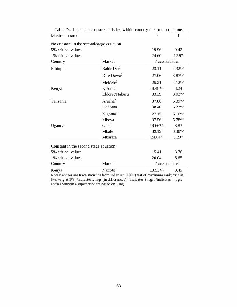
Step 3. Fuel price transmission from POE to other sub-national markets 14 Baltzer (2013) offers a useful summary of that literature.
12
We expect fuel prices in sub-national markets other than the POE to reflect POE prices plus domestic
transport costs. Deviations from this relationship – due to supply chain disruptions, localized fuel demand
shocks related to seasonality, or other forces – should not persist for long under reasonably competitive
conditions. Not surprisingly, Johansen tests clearly indicate the presence of a single cointegrating vector
between the POE market price of fuel and the fuel price in each non-POE market in the sample. In all
cases the Schwarz Bayesian criterion indicates an optimal lag length of two months in levels (therefore 1
month in differences). Accordingly, for each POE/other market pair, we estimate the following ECM:
(5) 𝐹𝑡𝑗
= 𝛼 + 𝛽𝐹𝑡𝑃𝑂𝐸 + 휀𝑡
(6) ∆𝐹𝑡𝑗
= 𝛿0𝐸𝐶𝑇𝑡𝑛𝑒𝑔
+ 𝛿1𝐸𝐶𝑇𝑡𝑝𝑜𝑠
+ 𝛿2∆ 𝐹𝑡−1𝑃𝑂𝐸 + 𝛿3∆𝐹𝑡−1
𝑗+ 𝜔𝑡
where 𝐹𝑡𝑗 is the fuel price in “other market” j, in month t, and all other terms are as described above. For
the within-country specifications we work entirely in nominal, local currency terms.
Step 4. Maize price transmission from POE to other sub-national markets
The final relationships of interest are those between POE maize prices and maize prices at sub-national
markets. Because crop transport in this region is conducted primarily via lorry, we allow fuel prices to
affect maize price spreads between the POE and other markets. As in the above sections, rank tests show
that in all specifications there is at most a single cointegrating vector between POE maize prices, other
market maize prices, and other market fuel prices, with an optimal lag of length of two months (in levels).
The error-correction framework takes the following form:
(7) 𝑀𝑡𝑗
= 𝛼 + 𝛽1𝑀𝑡𝑃𝑂𝐸 + 𝛽2𝐹𝑡
𝑗+ 휀𝑡
(8) ∆𝑀𝑡𝑗
= 𝛿0𝐸𝐶𝑇𝑡𝑛𝑒𝑔
+ 𝛿1𝐸𝐶𝑇𝑡𝑝𝑜𝑠
+ 𝛿2∆ 𝑀𝑡−1𝑃𝑂𝐸 + 𝛿3∆𝐹𝑡−1
𝑗+ 𝛿4∆𝑀𝑡−1
𝑗+ 𝜔𝑡
where 𝑀𝑡𝑗 is the price of maize in market j and all other variables are as before. The hypothesis 𝐻0 : 𝛽2 >
0 captures the expected effect of fuel prices on long-run maize price spreads.
We estimate all of the equations in Steps 2-4 using ordinary least squares. In some cases, after
initial estimation, we added lags to the second-stage equations to ensure white noise residuals (Enders
2010).
4. Results
Global Price Linkages
13
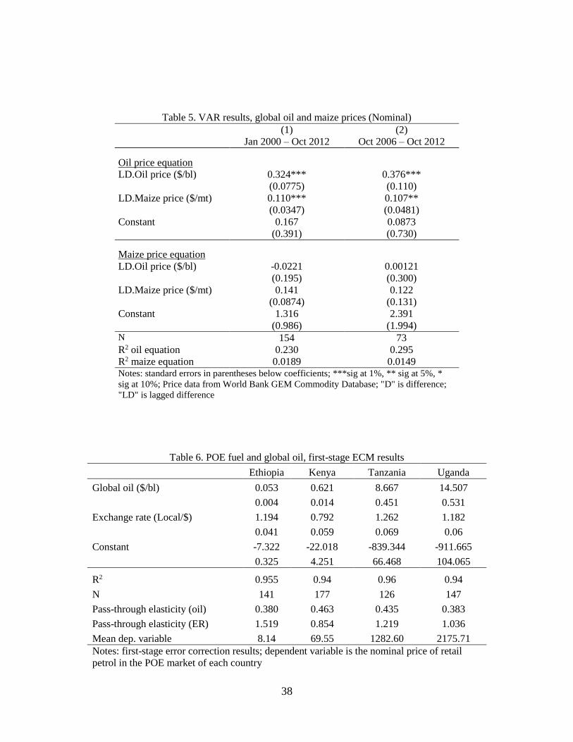
Table 5 shows the results of the reduced form VAR linking changes in oil and maize prices on global
markets. We show separate results for the periods January 2000 – October 2012 and October 2006 –
October 2012, in case the change in US ethanol policy affects the underlying inter-commodity price
relationship. We can reject the null of a unit root in the residuals for all equations (not shown). Coefficient
estimates are generally similar over the two periods. In neither period do maize prices exhibit a
statistically or economically significant response to lagged changes in oil prices. Maize prices are weakly
auto-correlated. Oil prices, however, demonstrate substantial auto-correlation, and positive changes in
maize prices tend to drive up oil prices. This is consistent with previous findings by Serra et al. (2011)
that corn price shocks cause increases in ethanol prices, which in turn induce adjustments in gasoline
prices, which feed back to crude oil markets.
While the estimates in Table 5 cannot be interpreted as causal, they do suggest that we can reject
a model in which global oil price movements directly affect maize price movements on the main
international market. This calls into question popular claims that global oil prices shocks trigger global
maize market adjustments. Of course, oil prices and maize prices may still co-move, either because of
correlated global commodity price shocks due to common underlying factors, as other recent studies have
found (Gilbert 2010, Enders and Holt 2012, Byrne et al. 2013), or because the relationship is nonlinear
and involves other variables, rendering it too nuanced for easy detection with our data and approach (de
Gorter et al. 2013). However, if global oil prices do have a positive but undetected effect on global maize
prices, that will only amplify the effects reported below.
Global-POE price transmission
Table 6 shows the estimates of equation 1, for all four countries. The final row of the table shows the
mean POE price over the study period, in local currency units. POE retail fuel prices are increasing in
both global oil prices and the exchange rate, as expected. Standard hypothesis testing on these
coefficients is not possible because the error term is nonstationary, therefore we do not provide stars
indicating statistical significance.
The key findings in Table 6 are summarized in the average pass-through elasticities for oil price
changes and exchange rate changes, which are listed in the lower half of the table. Estimates of POE
petrol price elasticities with respect to the global oil price are remarkably similar across countries. On
average, a 1% increase in the price of oil on world markets leads to an increase in the POE petrol price of
0.38-0.46%. Petrol price elasticities with respect to the exchange rate are higher and more variable,
ranging from 0.85 in Kenya to 1.52 in Ethiopia. Over the study period, slightly less than half of the
increase in nominal fuel prices in the POE markets is due to changes in nominal prices of global oil. The
remainder of the increase is driven by exchange rate depreciation.
14
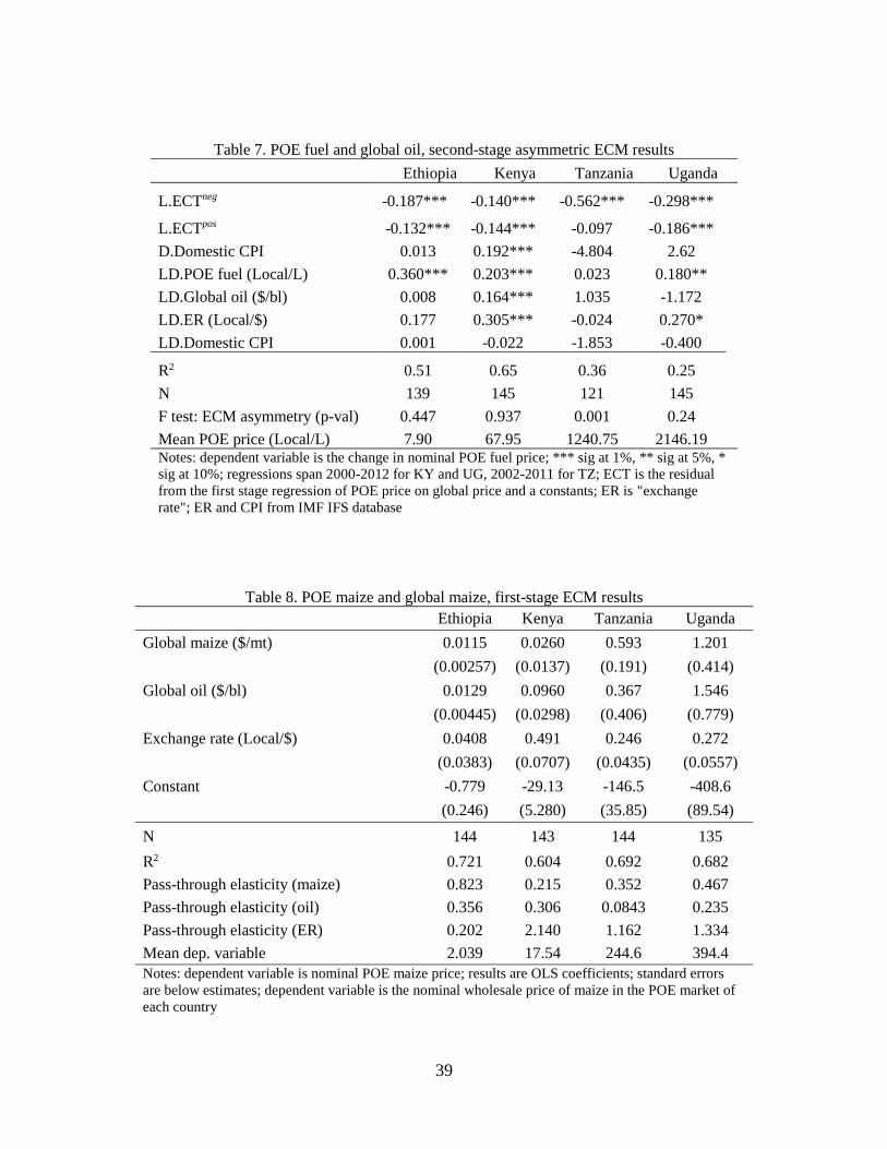
Table 7 shows the estimates of equation 2. All coefficient estimates have the expected sign, when
significant. Adjustment back to the long run equilibrium is not instantaneous, but is still reasonably fast
on average, with monthly adjustment rates ranging from 14-56%. Increases in global oil prices generally
transmit faster than do price decreases. However, F-tests for asymmetric adjustment indicate that only in
Tanzania is the difference statistically significant. This is consistent with various import bottlenecks, such
as port constraints, foreign exchange constraints, or contracting lags, and also with imperfect competition
in which importers adjust prices upward more quickly than downward.
Estimates of equation 3, the cointegrating vectors linking global maize prices to POE maize
prices, are reported in Table 8. POE maize–global maize pass-through elasticities (lower half of table)
exhibit greater heterogeneity than did the analogous POE petrol–global oil elasticities, ranging from 0.22
in Kenya to 0.82 in Ethiopia. These results correspond with an ordering of the degree to which central
governments intervene in maize markets, as Kenya’s more activist tariff and parastatal marketing board
policies translate into weaker transmission of global maize prices to the national market than in
neighboring countries. Pass-through elasticities of POE maize with respect to global oil prices are also
substantial, lying in the range 0.08-0.36, even after accounting for the direct impact of maize price
changes. In Kenya, by far the biggest maize importer in the region, a 1% increase in global oil prices
exhibits greater upward pressure on Mombasa POE maize prices (specifically, 0.31% increase) than does
a 1% increase in global maize prices (0.22%), underscoring the importance of transport costs to the
pricing of bulk grains. As with fuel prices, exchange rate elasticities vary widely, and are responsible for
any remaining changes in nominal POE maize prices after accounting for the direct impact of global
maize and global oil price changes.
In Figure 16 we plot the monthly average residuals from estimates of equation 3, normalized by
the overall mean POE maize price in each respective country. Seasonal patterns apparent in the deviations
from long-run equilibrium. These are consistent with intra-annual fluctuations in domestic supply, due to
the agricultural production cycle. For example, maize harvests in Ethiopia are concentrated in the months
September-November, which coincides with a drop in the Addis Ababa maize price vis-à-vis its long-run
relationship to the world price.
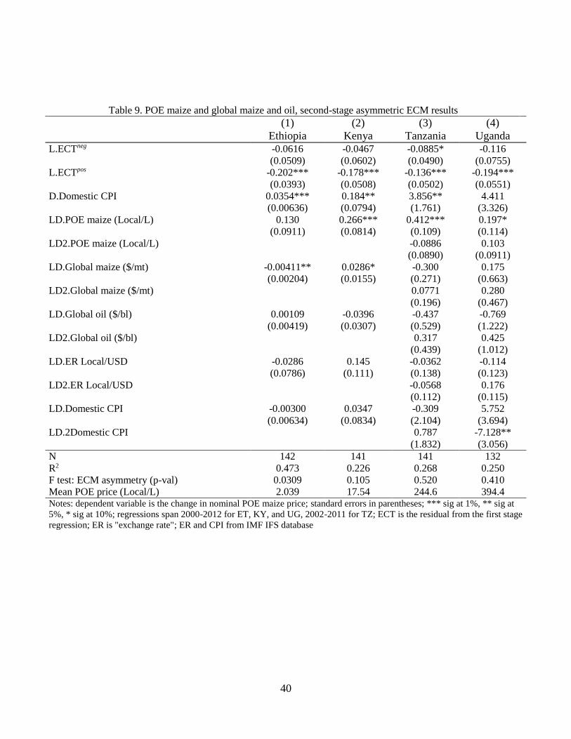
Second stage ECM results for the global-to-POE maize price relationship, based on equation 4,
are shown in Table 9. The error correction terms are highly significant in the wake of a positive deviation
from long-run equilibrium price (ECTpos), exhibiting the opposite pattern from the asymmetric models of
POE fuel prices. One interpretation of the asymmetric adjustment is that price arbitrage via exports is
logistically difficult due to port queues, regulatory barriers, the absence of short-term forward contracting,
and storage bottlenecks. On the other side, rapid recovery from higher prices may reflect the roles of food
aid, explicit export bans, and strategic release of grain reserves in mitigating the pace of food price
15
increases in the POE markets. Higher-than-equilibrium POE maize prices are generally absorbed in no
more than 6-8 months, with the arrival of the next harvest. Lower-than-equilibrium prices (ECTneg) persist
far longer. However, only in Ethiopia is the asymmetry statistically significant at the 5% level.
Coefficient estimates on lagged differences in global oil prices are not significant in any of the equations,
suggesting that changes in transport costs matter more for the long-run equilibrium (Table 8) than for
short-run price dynamics.
Within-country petrol price transmission
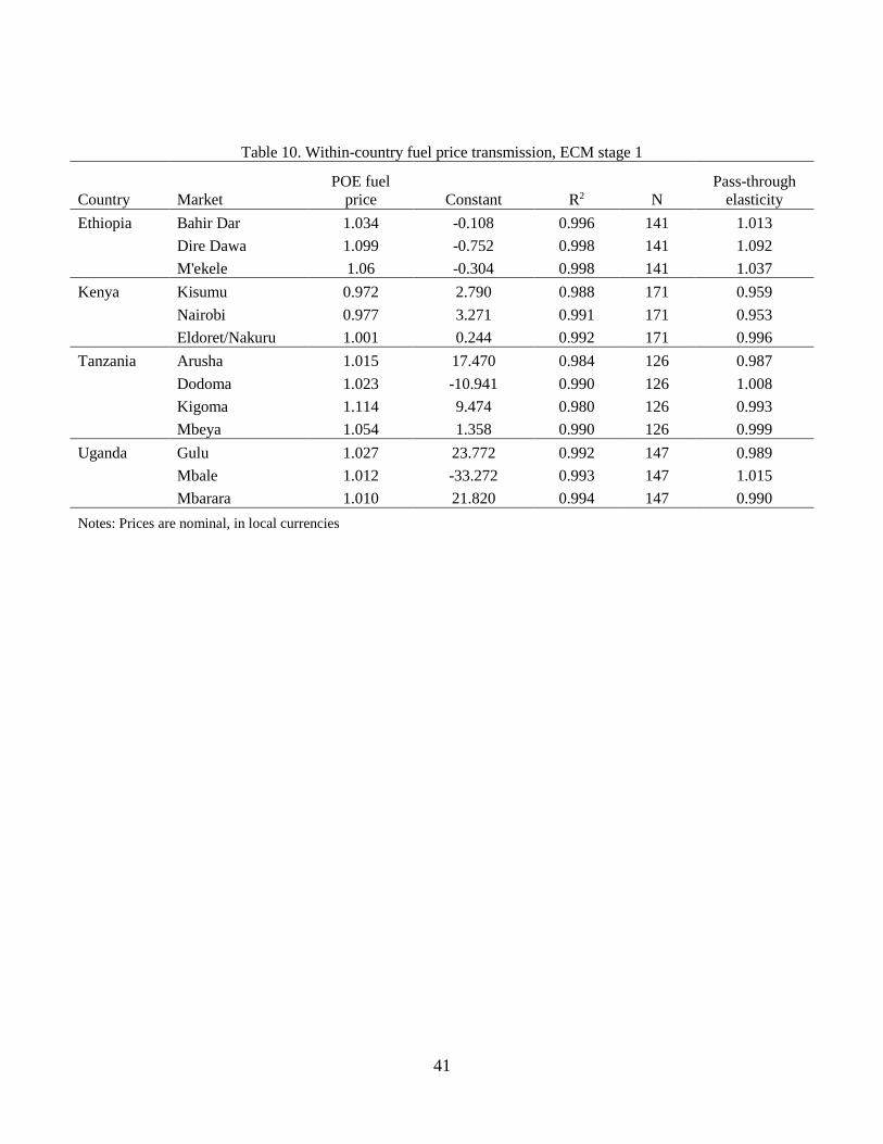
Table 10 shows the estimated co-integrating vectors based on equation 5, which link fuel prices in sub-
national markets to the POE fuel price. Most of the estimated models fit the data very closely. Fuel
markets are very well integrated within the study countries. The β coefficient estimates from equation 3
are all very close to unity, as are the estimated pass-through elasticities. This is clear empirical support for
the law of one price in fuel markets, which is expected given that ports-of-entry are the sole domestic
sources of liquid transport fuels in each country.
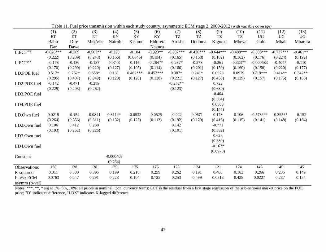
Second-stage ECM estimates, based on equation 6, are provided in Table 11. In all markets, POE
price increases transmit faster than POE price decreases. However, at 5% significance we can reject the
null of symmetric adjustment for only 2 of 13 markets. Faster pass-through of price increases could be
consistent with the existence of structural impediments to moving additional fuel quickly to non-POE
markets, or with imperfect competition among fuel distributors. Overall, equilibrium is restored very
rapidly when POE prices increase. Adjustment rates range from 31-74% in Ethiopia, Tanzania, and
Uganda. In Kenya, adjustment speeds are somewhat slower on average, though still rapid.
Within-country maize price transmission
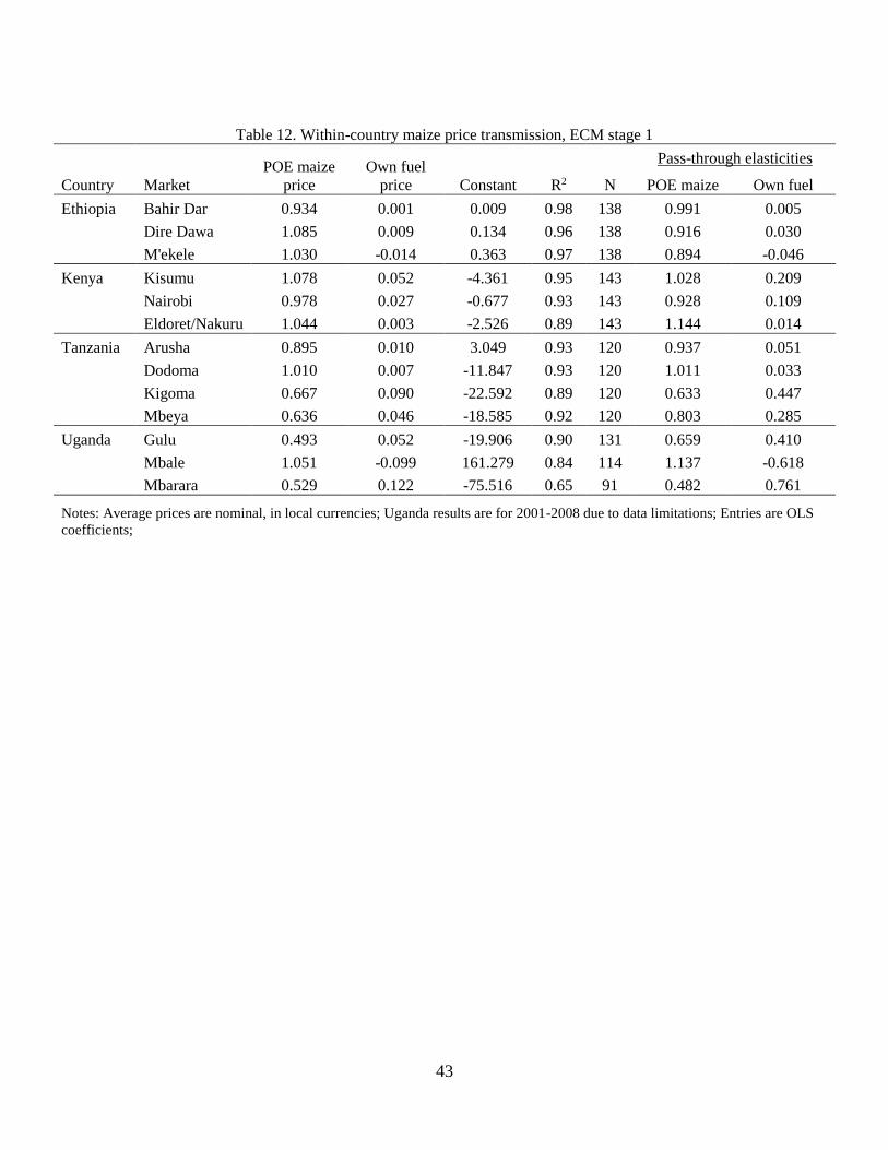
Table 12 shows the estimates of equation 7 for each of the sub-national markets. For 9 of 13 markets –
those in Ethiopia and Kenya, as well as Arusha, Dodoma, and Mbale – both the point estimates of 𝛽1 and
the POE maize price pass-through elasticities are close to unity, indicating conformity with the law of one
price. Within-country maize price elasticities are lower, in the 0.48-0.80 range, for the other four markets
in Tanzania and Uganda: Kigoma, Mbeya, Gulu, and Mbarara. These are the markets farthest from the
POE markets (Figure 4). These latter four markets also exhibit the largest positive pass-through
elasticities with respect to local fuel prices, ranging from 0.29 in Mbeya to 0.76 in Mbarara. In Mbarara
the estimated petrol price elasticity is higher than the POE maize price elasticity, and in Gulu and Kigoma
the estimated petrol price elasticity is approximately two thirds that of the maize price elasticity estimate.
In contrast, petrol price elasticities at Ethiopian markets, Arusha, Dodoma, and Eldoret/Nakuru
are all less than 0.06 in absolute magnitude. The outlier in Table 12 is the -0.62 petrol price elasticity in
16
Mbale. Because these coefficients must be interpreted with reference to the long run relationship between
the POE price and the sub-national market price, this suggests that increases in transport costs tend to
drive down the price of maize in Mbale relative to the price in Kampala. Because of its location near the
Kenya border, it is possible that Mbale receives some imports directly, bypassing Kampala entirely.
These results underscore the crucial role of transport to more remote markets, both in attenuating
food price pass-through and in augmenting the impact of global oil prices on transport costs. The
innermost markets in our study (Gulu, Mbarara, Kigoma, and arguably Mbeya) give some indication of
the likely impacts of oil price changes on food prices in land-locked nations and remote trading towns. In
these markets, transport costs are as or nearly as important as POE maize prices in determining maize
prices. Figure 16 depicts the clear positive relationship between the estimated elasticities of local maize
prices with respect to global oil prices as a function of distance from POE. Conversely, in Figure 17 we
plot the estimated elasticities of local maize prices with respect to global maize prices as a function of
distance from the market nearest the domestic maize surplus zone (the “breadbasket”). The clear positive
relationships between distance and estimated pass-through rates, in both figures, highlight the importance
of transport costs in local maize price determination.
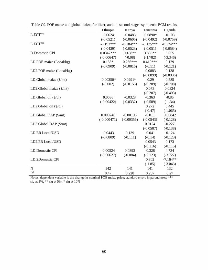
In Table 13 we report the second-stage results of the asymmetric ECM based on equation 8. Once
again, all of the ECT coefficients have the expected, negative sign (apart from the coefficient on
𝐿. 𝐸𝐶𝑇𝑡𝑝𝑜𝑠
in the Mbale equation, which is not statistically significant). Adjustment back to equilibrium is
reasonably fast, with rates ranging from 19-92% per month, consistent with prior findings for Tanzania
maize markets (van Campenhout 2007). Many of the maize price series demonstrate positive
autocorrelation, and likewise respond positively in the short-run to lagged changes in the POE maize
price. Asymmetries in adjustment are only statistically significant in Dire Dawa and Mbale. Just as with
the global-POE adjustment processes, fuel prices have little effect on the short run dynamics; only 2 of 13
markets have a statistically significant, positive point estimate on lagged fuel price in the maize ECM
regressions. In the breadbasket markets of Bahir Dar, Gulu and Mbeya, the (albeit statistically
insignificant) short term impact of a fuel price increase is to decrease local maize prices, likely because of
temporary reductions in the profitability of transporting maize away from these markets. Overall,
however, fuel prices play a larger role in determining the long run spatial equilibrium price relationships
(Table 12) than in mediating adjustments to those equilibria (Table 13).
5. Discussion
The estimated pass-through elasticities from the preceding section tell us about relationships between
price pairs. But if we want to estimate the full impact of a global oil price increase on sub-national maize
market equilibrium prices in east Africa, we need to integrate our estimates of the co-integrating vectors
17
that describe the long-run stationary relationships among various price series. Because we find no
statistically significant impact of global oil prices on global maize prices, consistent with much of the
prior literature, we assume away any transmission through that pathway (although we will consider
scenarios in which maize and oil prices co-move). Note that any positive effect of global oil prices on
global maize prices, due perhaps to diversion of grain supply from food and feed markets to fuel markets,
would only reinforce our core findings that global oil markets significantly maize prices in east Africa.
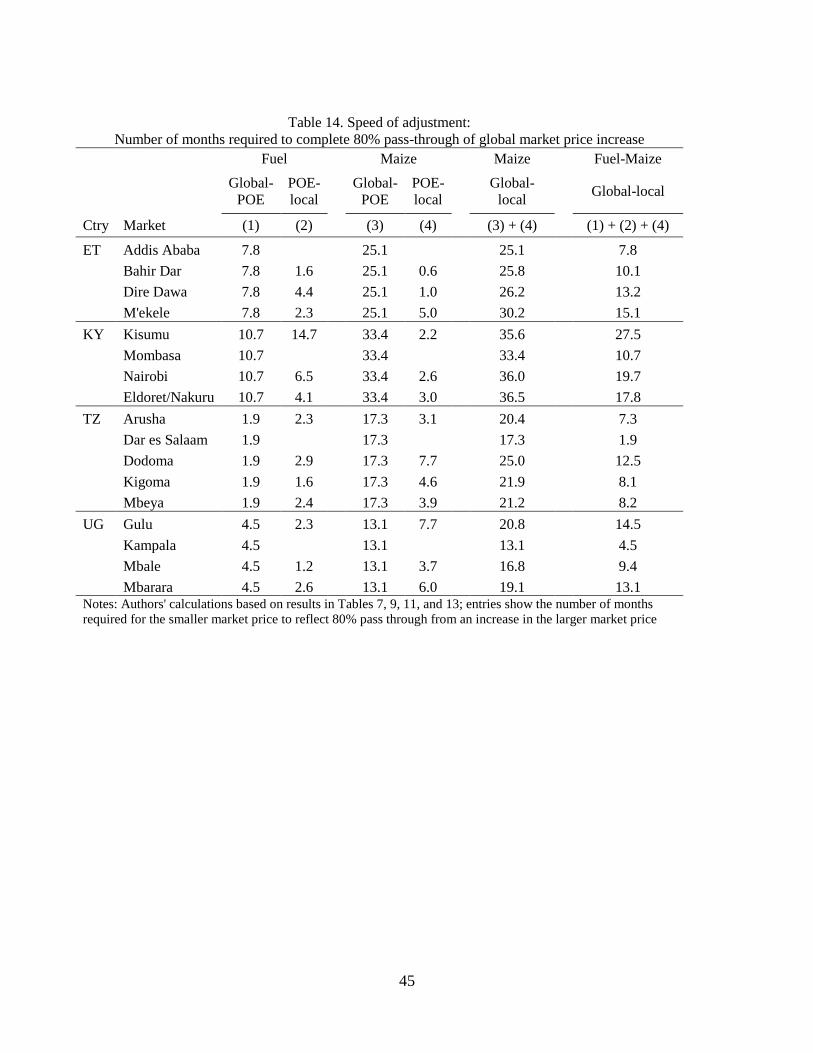
We report above that fuel price shocks transmit much more rapidly within the four study
countries than do maize price shocks. Table 14 summarizes the speed-of-adjustment findings by showing
the number of months needed to absorb 80% of a price increase. In all four countries, it takes substantially
longer to return to POE maize price equilibrium after a global maize price rise than it does to return to
POE petrol price equilibrium following a global oil price rise (compare columns 1 and 3). Likewise, in
Tanzania and Uganda, where governments intervene less in fuel markets than in Ethiopia or Kenya, POE
petrol price changes transmit more rapidly within the country than do POE maize price changes (compare
columns 2 and 4).
The implication of this pattern is that in the face of correlated increases in global maize and oil
prices, increases in transport costs drive up sub-national maize prices across east Africa more quickly than
do the direct pass-through effects of higher grain prices on global markets. This is most clear from a
comparison of the two rightmost columns in Table 14, which show the sums of columns 3 and 4, and of
columns 1, 2, and 4, respectively.15 In all cases, sub-national maize market prices converge to their new
long-run equilibrium substantially faster in response to a global oil price shock than to a global maize
price shock. In 11 of 17 markets, the number of months needed to absorb an oil price rise is less than half
of that needed to absorb a global maize price rise. While it is not surprising that adjustment speeds are
slower for a good that is produced domestically and sometimes subject to government intervention on
food security grounds (such as ad hoc export bans), the magnitude of the difference is striking.
Of course, rapid pass-through of fuel price increases matters only insomuch as the impact of
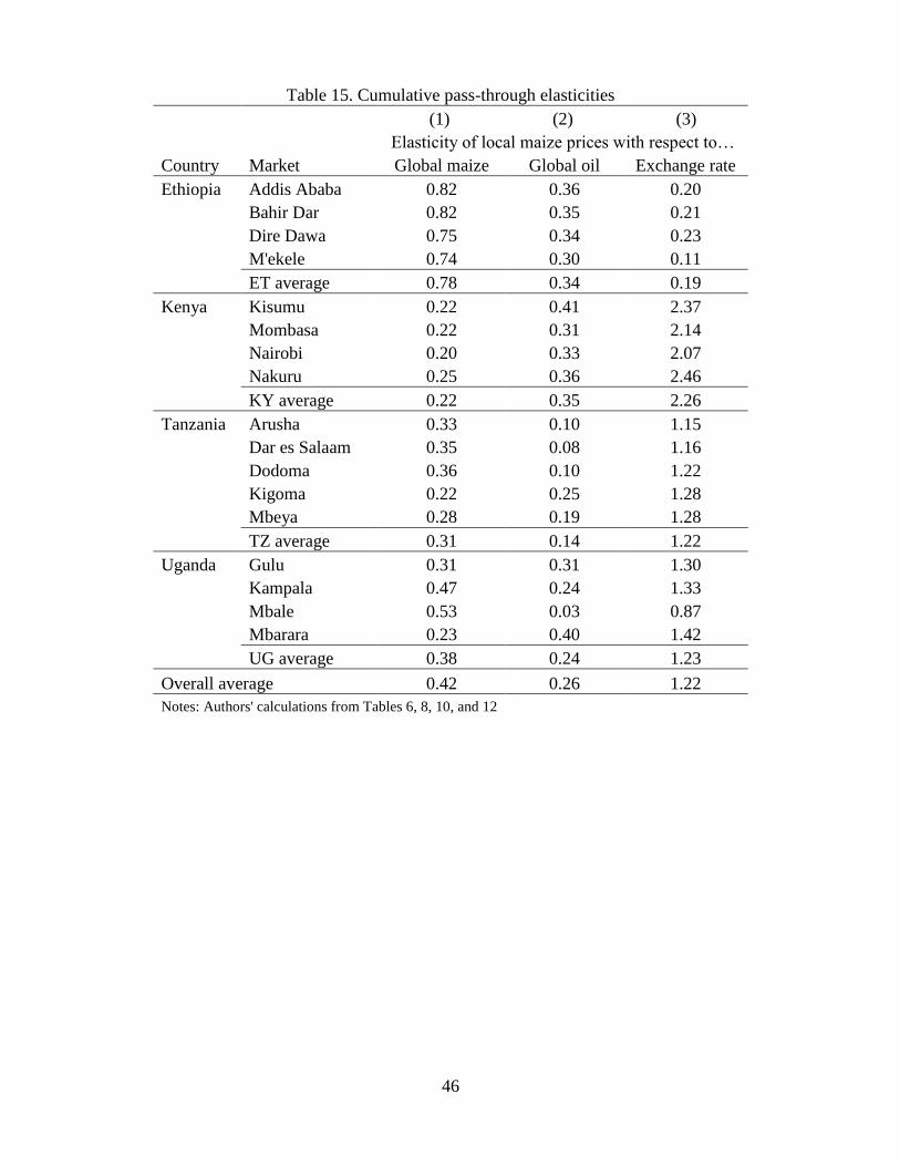
global oil price increases on local maize prices is of significant magnitude. It is. Table 15 reports the
estimated cumulative pass-through elasticities of local maize prices with respect to increases in global
maize prices, global oil prices, and exchange rates, based on the findings in Tables 6, 8, 10 and 12.16
Local maize price elasticities with respect to global maize prices (column 1) are highest in
Ethiopia (0.74-0.82), and lower but still substantial in the other three countries, ranging between 0.20-
0.25 in Kenya, 0.22-0.36 in Tanzania, and 0.23-0.53 in Uganda. In Table 12 we saw that within each
country, long-run spatial equilibrium in maize prices routinely corresponded with the predictions of the
15 Note that these are upper bounds on the speed of convergence to long-run equilibria. By directly adding the
previous columns we implicitly assume that adjustment occurs sequentially rather than simultaneously. 16 Entries in Table 15 are the products of the elasticities from the relevant links in the supply chain (see Figure 14).
18
law of one price, consistent with a longstanding literature (Engel and Rogers 1996, Evans 2003, Anderson
and van Wincoop 2004). It is the impact of trade across international frontiers (Table 8) which dampens
maize-to-maize price transmission in Table 15.
In column 3 we see that exchange rate elasticities vary considerably across countries, from very
low estimates in Ethiopia (0.11-0.23) to substantially greater figures in Kenya (2.07-2.46). At the country
level these estimates are ordered inversely from the global maize price elasticities in column 1, hinting at
the role of macroeconomic adjustment to external terms of trade shocks in determining local equilibrium
prices. In fact, these cross-country differences likely reflect differences in the importance of maize in the
general price indices (which then impacts the equilibrium exchange rate). Maize is most critical to
consumption in Kenya, and that is where we see exchange rate adjustment having a substantially larger
effect on equilibrium maize prices than it does in the other countries.
The findings in Table 15 that are most central to this paper are the cumulative impacts of global
oil price changes on local maize prices, in column 2. In all of the markets in Kenya, as well as in the more
remote markets of Gulu and Mbarara, in Uganda, and Kigoma, Tanzania, cumulative pass-through maize
price elasticities from global oil price increases are greater than those from global maize price increases.
In Mbeya, Tanzania, one of the other remote trading centers in the study (though still a major maize
producing region), the estimated global oil price elasticity of 0.19 is two thirds of the estimated global
maize price elasticity (0.28). For markets in Ethiopia, as well as Kampala, Arusha, and Dar es Salaam (the
largest cities in Uganda and Tanzania), cumulative elasticities with respect to global oil prices are a little
less than half the magnitude of those with respect to global maize prices. Across the sample, the average
global maize price elasticity is 0.42, while the average global oil price elasticity is 0.26.17 Recall that these
global oil price elasticities assume no link between oil and maize prices on global markets; any such link
would indicate that the true average elasticity of local maize prices to global oil prices is greater than
0.26. This underscores the often-underappreciated importance of variable transport costs in determining
equilibrium food prices in infrastructure-deficient Africa.
Kenya is the only study country in which estimates of local maize price elasticities with respect to
global oil prices are systematically greater than those with respect to global maize prices. Kenya is also
the only study country in which farmers applied substantial amounts of inorganic fertilizers during the
study period. Because much inorganic fertilizer production relies on natural gas feedstock, the price of
which is closely linked to the price of oil on global markets, this raises the possibility that the link
17 These estimated pass-through rates significantly exceed IMF (2009) findings that only 3-21% of global food price
shocks transmit to food prices within Kenya, Tanzania or Uganda, and that the pass through rate of world oil prices
to domestic food prices is only 11% in Uganda and statistically insignificantly different from zero for Kenya and
Tanzania. However, the IMF findings are based on simpler vector autoregression methods that do not account for
the nonstationarity of the series, and use aggregate national price series rather than market-specific prices.
19
between global oil prices and Kenya maize prices may be partly mediated through an increase in domestic
maize production costs, rather than transport costs. Such an impact would not be expected to persist
indefinitely because in the long run Kenya maize prices are tied to global maize prices, which should be
invariant to production costs in Kenya, a very small producer in global terms. Nonetheless, in a
robustness check we explore this potential channel because of the notable qualitative difference between
the results for Kenya and those for the other study countries, as well as the fact that Kenya is the only
study country where fertilizer use on maize is widespread. Were we to find that fertilizer costs have a
substantial impact on Kenya maize prices, a potential (though unlikely) alternative to the transport costs
interpretation of our core results is that maize markets near Mombasa are served primarily by imports,
while maize markets in the western population centers of Kenya are served by local production that relies
on inorganic fertilizer.
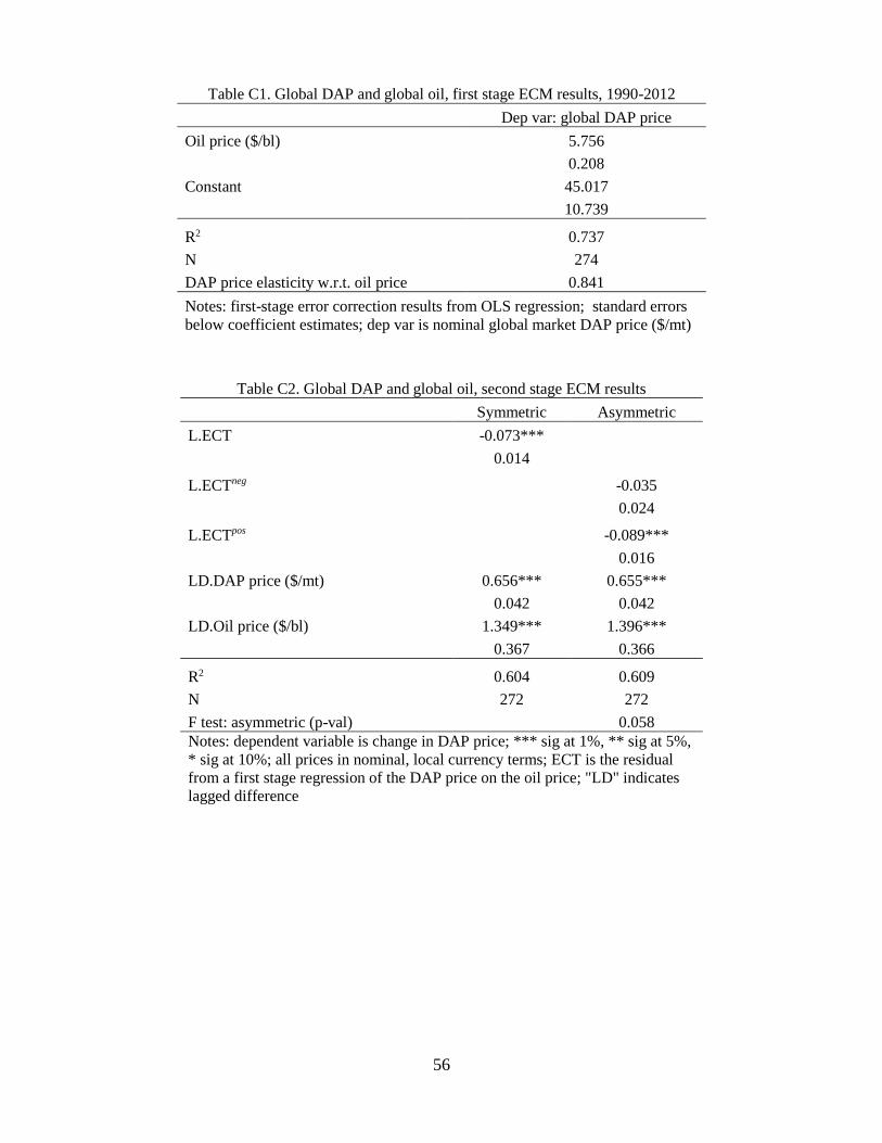
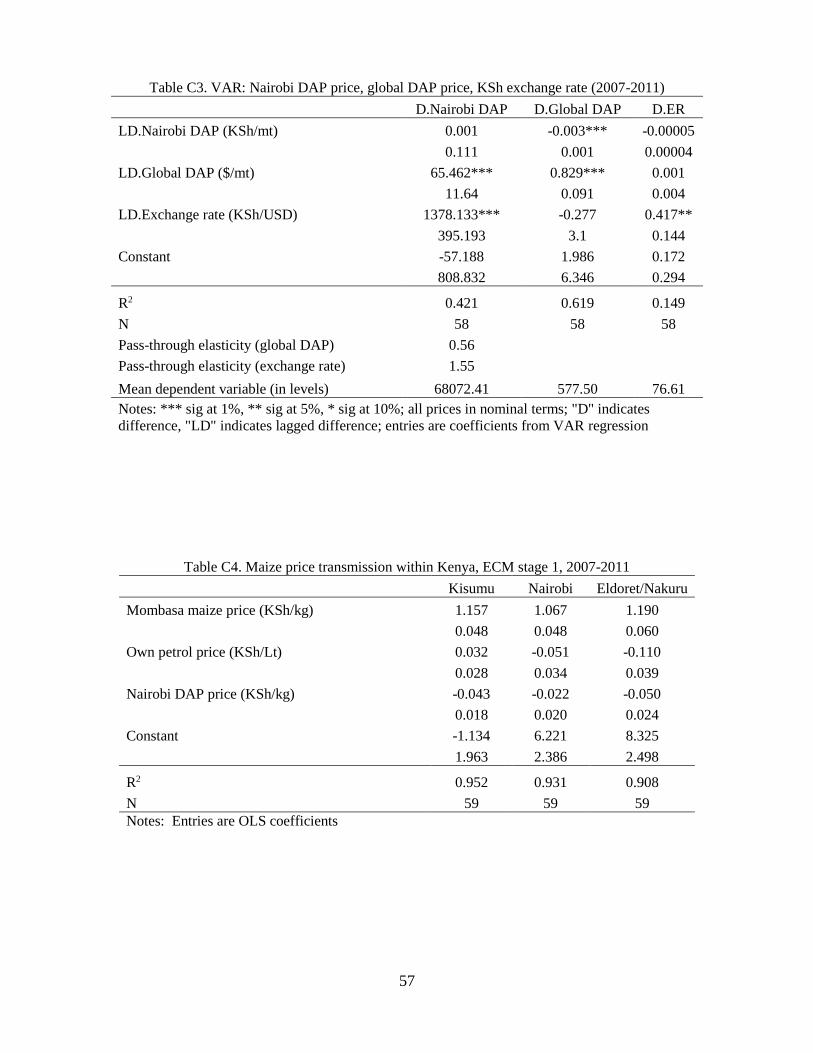
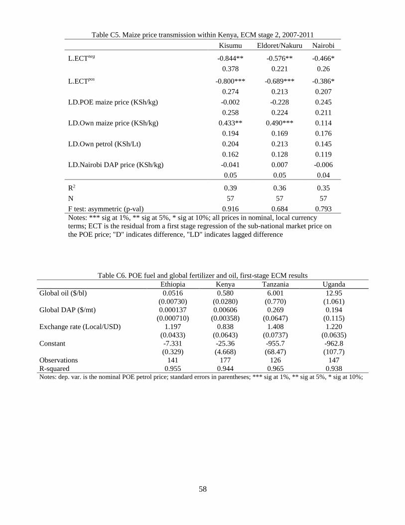
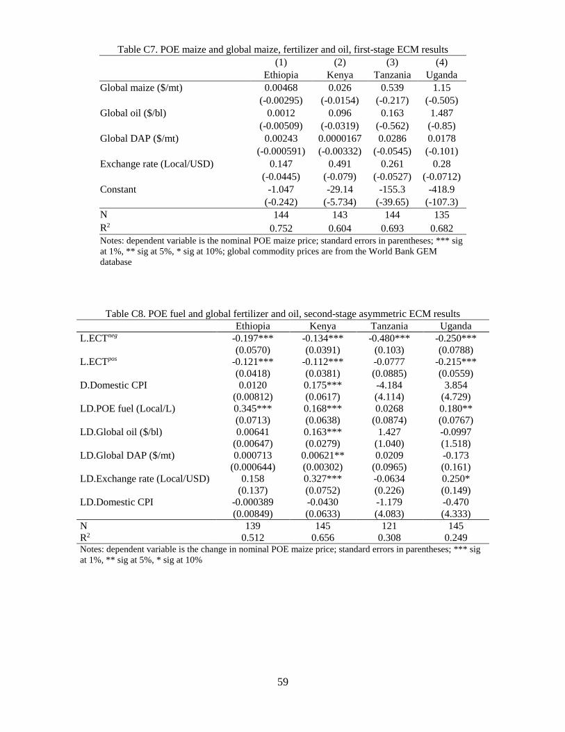
However, using a limited (though best available) monthly time series of Kenya fertilizer prices,
which includes monthly average di-ammonium phosphate (DAP) prices in Nairobi for the period 2007-
2011, we find no impact of domestic fertilizer prices on equilibrium maize prices in Kenya (see Appendix
C for details). At the global level there is a clear link between oil prices and fertilizer prices,18 but this
does not influence maize prices in east Africa independently of whatever effects are mediated through the
price of maize on global markets.
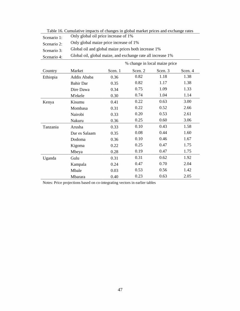
Finally, Table 16 shows the full impact on local maize prices from four price change scenarios.
Scenarios 1 and 2 directly correspond to the price changes that implicitly underlie the elasticities
presented in Table 15: a 1% increase in the global oil price and a 1% increase in the global maize price,
respectively. The third scenario considers a generalized increase in global commodity prices that
generates correlated 1% price rises for both crude oil and maize (following Gilbert 2010, Enders and Holt
2012 or Byrne et al. 2013). Lastly, the fourth scenario incorporates possible macroeconomic impacts on
exchange rates due to changes in the prices of tradables, by assuming that global oil prices, global maize
prices, and exchange rates all increase 1% over their baseline values. Scenarios 3 and 4, therefore, provide
bounds on the total effect allowing for zero and complete exchange rate adjustment, respectively. Because
correlated commodity price movements are commonplace (Gilbert 2010, Enders and Holt 2012, Byrne et
al. 2013, Baffes and Dennis 2013), we consider scenarios 3 and 4 to be the most realistic.
We use an additive linear framework to model long-run relationships, therefore estimates under
scenario 3 are the sum of those under scenarios 1 and 2. Aggregate pass-through rates in response to
perfectly correlated global maize and oil price shocks are high: over 100% pass-through in Ethiopia, 52-
63% in Kenya, 43-47% in Tanzania, and 56-70% in Uganda. These estimated changes occur in the
absence of any changes in the exchange rate.
18 Results available upon request.
20
When the exchange rate depreciates by 1% as well, in scenario 4, the cumulative local maize
price elasticities are all greater than unity. In most Ugandan markets the estimated elasticity approaches 2,
and estimates are in the 2.61-3.06 range across Kenyan markets. These are upper bounds on true pass-
through elasticities, since they are premised on an out-of-equilibrium simulation of an exchange rate
change.19 However, the interesting finding in scenario 4 is the disparity in the relative importance of
exchange rate changes across the study countries. In Ethiopia, real domestic prices are closely matched to
real global prices, so that exchange rate adjustment has only a minor effect on pass-through rates.
Exchange rate effects in Kenya, on the other hand, are especially pronounced (as noted earlier).
The broad implication of our findings is that both global oil and global maize prices exert
considerable influence on sub-national maize prices across east Africa. Although cross-border price
transmission is less complete than that within countries – which largely follows the law of one price in
long-run equilibrium for both fuel and maize – the most narrow estimates, assuming global oil price
shocks are uncorrelated with global maize prices and exchange rates, still suggest a pass-through ratio of
0.26, while more realistic estimates that allow for such correlation quickly approach or exceed 1. Equally
importantly, global oil prices seem to impact sub-national maize prices through transport cost effects, not
by inducing changes in global maize prices nor by driving up local costs of farm-level production,
although these latter two are the pathways most frequently discussed in the literature and the popular
press. These estimated magnitudes and the fact that local maize price adjustment to global oil market
shocks occurs much faster than it does to global maize market shocks both suggest that researchers and
policymakers concerned about the food price effects of oil market shocks ought to pay more attention to
transport systems and their variable costs.
6. Conclusions
The potential of global crude oil price shocks to disrupt food markets in developing countries naturally
concerns astute observers, given experiences over the past half dozen years. In this paper we explore
those linkages systematically. We first look at inter-commodity oil-maize price transmission in global
markets. Then we estimate spatiotemporal price transmission from global crude oil markets to national
and sub-national petrol fuel markets in east Africa, and then repeat the exercise for maize markets,
allowing oil prices to influence maize prices independently as a way to capture the prospective effects of
variable transport costs. To the best of our knowledge, this is the first study to explore both inter-
commodity and intra-national price transmission from oil to cereals markets. Moreover, it brings out how
the mechanisms that might lead global oil prices to influence maize prices in the United States – primarily
19 See Adam (2011) or Arndt (2013) for macroeconomic models of the simulated effects of external food prices
shocks, allowing for equilibrium adjustment in exchange rates.
21
through ethanol markets and by induced changes in farm input costs for fertilizer and fuel20 – may differ
dramatically from those that influence maize prices in low-income agrarian countries in Africa or other
low-income regions where transport costs may be the primary channel of influence.
Like several studies before ours, we find no statistically significant causal relationship from oil
prices to maize prices on global markets. By contrast, there exist strong, long run equilibrium
relationships between global and national prices in both fuel and maize markets. Global prices clearly
transmit to national level markets, with fairly high rates of pass-through. Within countries, there are even
stronger price transmission patterns, most of them conforming to the law of one price hypothesis that
price adjustments in one market transmit one-for-one to others in long-run equilibrium, controlling for
transport costs. Furthermore, domestic fuel markets transmit price increases quickly, with adjustments to
a new long-run equilibrium typically taking place within just a few months. The transmission from global
maize markets to domestic maize markets is considerably slower, likely owing to policy interventions and
infrastructural bottlenecks that impede international arbitrage.
The estimates derived from these time series price analyses permit us to estimate the impact of an
increase in global oil prices on local maize prices in sub-national markets across east Africa. We find
clear evidence that global oil prices indeed exert some influence on sub-national maize prices across east
Africa through transport cost effects. These effects can be significant. The average estimated local maize
price elasticity with respect to the global crude oil price is 0.26, with the greatest effects felt in the most
remote markets. This novel finding underscores the importance of considering the full food system,
including post-harvest distribution networks and their associated costs, in thinking through the food
security implications of global shocks.
The co-movement of grain and oil prices on global market can obscure the important role of
transport costs in exacerbating the negative consequences of food price shocks. In the study markets
farthest from coastal ports, fuel price increases put greater upward pressure on local maize prices than do
maize prices at the port-of-entry. More generally, the elasticity of local market maize prices with respect
to global oil prices increases with distance from port of entry.
This finding has important policy implications. For landlocked regions of the low-income world,
policies to mitigate the negative consequences of grain price shocks by directly intervening in both
transport and grain markets, rather than just the latter, are more likely to achieve the desired food security
objectives. Increased high-level attention to global food security tends to focus on farm-level productivity
growth and on safety nets for poor consumers. Although these are clearly high priorities, so too is it
essential to increase efficiency in the post-harvest systems – including liquid fuels and transport – that
20 Mitchell (2008) reports that in 2007, combined chemical, energy and fertilizer costs accounted for 34% of maize
production costs in the United States and these costs move sharply in response to oil prices.
22
deliver food to rapidly urbanizing populations from both domestic farmers and international markets
(Gómez et al. 2011).
References
Abbott, P. C., C. Hurt, W.E. Tyner (2008). What’s Driving Food Prices? Oak Brook, IL: Farm
Foundation.
Abbott, P, A Borot de Battisti (2011). “Recent Global Food Price Shocks: Causes, Consequences and
Lessons for African Governments and Donors”, Journal of African Economies 20(s1): i12-i62.
Adam, C (2011). “On the Macroeconomic Management of Food Prices Shocks in Low Income
Countries”, Journal of African Economies 20: 63-99.
Anderson, H.M. (1997). “Transactions Costs and Nonlinear Adjustment in Real Exchange Rates: An
Empirical Investigation.” Oxford Bulletin of Economics and Statistics 59(4): 465-484.
Anderson, J.E., E van Wincoop (2004). Trade Costs. Journal of Economic Literature 42(3): 691–751.
Ardeni, P.G., B.D. Wright (1992) "The Prebisch-Singer Hypothesis: A Reappraisal Independent of
F test: ECM asymmetry (p-val) 0.0309 0.105 0.520 0.410
Mean POE price (Local/L) 2.039 17.54 244.6 394.4 Notes: dependent variable is the change in nominal POE maize price; standard errors in parentheses; *** sig at 1%, ** sig at
5%, * sig at 10%; regressions span 2000-2012 for ET, KY, and UG, 2002-2011 for TZ; ECT is the residual from the first stage
regression; ER is "exchange rate"; ER and CPI from IMF IFS database
Table 11. Fuel price transmission within each study country, asymmetric ECM stage 2, 2000-2012 (with variable coverage) (1) (2) (3) (4) (5) (6) (7) (8) (9) (10) (11) (12) (13) ET ET ET KY KY KY TZ TZ TZ TZ UG UG UG
Notes: ***, **, * sig at 1%, 5%, 10%; all prices in nominal, local currency terms; ECT is the residual from a first stage regression of the sub-national market price on the POE
Notes: ***, **, * sig at 1%, 5%, 10%; all prices in nominal, local currency terms; ECT is the residual from a first stage regression of the sub-national market price on the POE price; "D"
Notes: *** sig at 1%, ** sig at 5%, * sig at 10%; all prices in nominal, local currency
terms; ECT is the residual from a first stage regression of the sub-national market price on
the POE price; "D" indicates difference, "LD" indicates lagged difference
Table C6. POE fuel and global fertilizer and oil, first-stage ECM results
Ethiopia Kenya Tanzania Uganda
Global oil ($/bl) 0.0516 0.580 6.001 12.95
(0.00730) (0.0280) (0.770) (1.061)
Global DAP ($/mt) 0.000137 0.00606 0.269 0.194
(0.000710) (0.00358) (0.0647) (0.115)
Exchange rate (Local/USD) 1.197 0.838 1.408 1.220
(0.0433) (0.0643) (0.0737) (0.0635)
Constant -7.331 -25.36 -955.7 -962.8
(0.329) (4.668) (68.47) (107.7)
Observations 141 177 126 147
R-squared 0.955 0.944 0.965 0.938 Notes: dep. var. is the nominal POE petrol price; standard errors in parentheses; *** sig at 1%, ** sig at 5%, * sig at 10%;
59
Table C7. POE maize and global maize, fertilizer and oil, first-stage ECM results
(1) (2) (3) (4)
Ethiopia Kenya Tanzania Uganda
Global maize ($/mt) 0.00468 0.026 0.539 1.15
(-0.00295) (-0.0154) (-0.217) (-0.505)
Global oil ($/bl) 0.0012 0.096 0.163 1.487
(-0.00509) (-0.0319) (-0.562) (-0.85)
Global DAP ($/mt) 0.00243 0.0000167 0.0286 0.0178
(-0.000591) (-0.00332) (-0.0545) (-0.101)
Exchange rate (Local/USD) 0.147 0.491 0.261 0.28
(-0.0445) (-0.079) (-0.0527) (-0.0712)
Constant -1.047 -29.14 -155.3 -418.9
(-0.242) (-5.734) (-39.65) (-107.3)
N 144 143 144 135
R2 0.752 0.604 0.693 0.682
Notes: dependent variable is the nominal POE maize price; standard errors in parentheses; *** sig
at 1%, ** sig at 5%, * sig at 10%; global commodity prices are from the World Bank GEM
database
Table C8. POE fuel and global fertilizer and oil, second-stage asymmetric ECM results