GLOBAL DEVELOPMENT, TRADE, HUMAN CAPITAL, AND …

Oradea Journal of Business and Economics, Volume V, Special Issue Published on June 2020

9

GLOBAL DEVELOPMENT, TRADE, HUMAN CAPITAL, AND BUSINESS CYCLES Wei-Bin Zhang Ritsumeikan Asia Pacific University, Japan [email protected] Abstract: This paper generalizes the multi-country growth model with capital accumulation, human capital accumulation, economic structure and international trade by Zhang (2014) by making all the time-independent parameters in Zhang’s model as time-dependent parameters. Each national economy consists of one tradable, one non-tradable and one education sector. National economies are different in propensities to save, to obtain education and to consume, and in learning abilities. The model integrates the Solow growth model, the Uzawa two-sector growth model, the Uzawa-Lucas two-sector growth model, and the Oniki–Uzawa trade model within a comprehensive framework. Human capital accumulation is through education in the Uzawa-Lucas model, Arrow’s learning by producing, and Zhang’s learning by consuming (creative learning). The behavior of the household is described with an alternative approach to household behavior. We simulated the model to demonstrate existence of equilibrium points, motion of the dynamic system, and oscillations due to different exogenous shocks. Keywords: trade pattern, education, non-tradable, economic oscillations, wealth accumulation JEL classification: F1, F43, F44, J24, J11. 1. Introduction This paper is concerned with identifying economic fluctuation in a synthesized Solow-Uzawa’s growth, Oniki-Uzawa trade, and Lucas-Uzawa’s two-sector model with exogenous shocks. The model is based on Zhang’s model (Zhang, 2014). The main generalization of this study is to treat all the time-independent parameters in Zhang’s model as time-dependent. This will make Zhang’s original model far more robust as there are many factors, such as technological change, institutional shifts, fashions, seasonal factors, are time-dependent and are considered exogenous. Economics oscillations, often referred as business cycles, are commonly observed in empirical studies. Some researches consider economic oscillations as exogenous. A typical example is agricultural production which is influenced by seasonal changes as well as long-term global climates. Oscillations may also occur in a self-organized economic system without any exogenous influences. There are a lot of theoretical and empirical research about mechanisms and phenomena of economic fluctuations (e.g., Zhang, 1991, 2005, 2006; Lorenz, 1993; Flaschel et al 1997; Chiarella and Flaschel, 2000; Shone, 2002; Gandolfo, 2005; Puu, 2011; Nolte, 2015). These studies show how modern dynamic analysis can be applied to different economic systems, identifying existence of cycles, regular as well as irregular oscillations, and chaos in economic systems. There are also other studies which try to explain economic business cycles from different perspectives. Lucas (1977) demonstrates possible existence of some shocks that affect all sectors in an economy. Chatterjee and Ravikumar (1992) build a neoclassical growth model with seasonal perturbations to taste and technology. They demonstrate how the economic system reacts to seasonal demand and supply perturbations. Gabaix (2011) holds that uncorrelated sectoral shocks are determinants of aggregate fluctuations (see also, Giovanni,


10

et al. 2014; Stella, 2015). This study attempts to make a contribution to the literature by identifying economic fluctuations in a trade model with endogenous physical and human capital. This paper is based on a model recently proposed by Zhang (2014). Zhang’s model deals with dynamic interdependence between wealth and physical capital accumulation, human capital accumulation, and trade patterns in a multi-country neoclassical growth theory framework. The basic economic mechanism of wealth accumulation based on the Solow growth model with an alternative approach. International trade follows the trade models with accumulating capital developed by Oniki and Uzawa and others (for instance, Oniki and Uzawa, 1965; Frenkel and Razin, 1987; Sorger, 2002; and Nishimura and Shimomura, 2002). The analytical framework of the Oniki-Uzawa model is important for analyzing interdependence between trade patterns and economic growth. The Oniki-Uzawa model should be extended as it is constructed for the two-country with two goods. In fact, most of trade models with endogenous capital are still either limited to two-country or small open economies without taking account of endogenous human capital. Rather than classifying capital goods and consumer goods as in the Oniki-Uzawa model, we use tradable good and non-tradable. Distinction between tradable good and non-tradable good is significant for explaining many economic issues. There are analytical frameworks with tradable and non-tradable goods for explaining the terms of trade (Mendoza, 1995), for examining exchange rates (Stulz, 1987; Stockman and Dellas, 1989; Backus and Smith, 1993; Rogoff, 2002; Raleva, 2013); for dealing with current account dynamics (Edwards, 1989; Hohberger, et al. 2014), for examining investment structure (Cachanosky, 2014); or for solving the home premium puzzle (Baxter et al., 1998; Pesenti and van Wincoop, 2002). Backus and Smith (1993:1) explains this distinction as follows: “The mechanism is fairly simple. Although the law of one price holds, in the sense that each good sells for a single price in all countries, PPP may not: price indexes combine prices of both traded and nontraded goods, and because the latter are sold in only one country their prices, and hence price indexes, may differ across countries.” Stockman and Tesar (1995) observe that the tradable sector is generally more volatile. Zhao et al. (2014) explains the difference between the tradable and non-tradable sectors by introducing labor adjustments in response to impulses. According to Zhao et al. (2014: 230) “Tradable sector variables like capital, investment, consumption and output are more volatile than their nontradable counterparts. This is especially true for output, where the tradable sector is more than two times as volatile. The nontradable sector accounts for almost half of both GDP and total consumption. Understanding the sources of volatility by sector may help in understanding the sources of aggregate fluctuations, the effects of shocks on the aggregate economy, and the likely impact of alternative public policies.” The study treats differences in human capital between countries as endogenous variables. Dynamic interdependence between economic growth and human capital is important for explaining national differences in growth and income (e.g., Easterlin, 1981; Hanushek and Kimko, 2000; Barro, 2001; Krueger and Lindahl, 2001; Galor and Zeira, 1993; Castelló-Climent and Hidalgo-Cabrillana, 2012; Barro and Lee, 2013; and Hanushek et al. 2014). This study considers three sources of learning – education in the Uzawa-Lucas model, Arrow’s learning by doing, and Zhang’s learning by consuming (which include leisure, family conditions, travels and readings at leisure, and so on). The first formal dynamic growth model with education was proposed by Uzawa (1965). There is an extensive literature on education and economic growth (Mincer, 1974; Tilak, 1989; Could et al., 2001; Tselios, 2008; Fleisher et al. 2011; Zhu, 2011). There is also a large number of the theoretical literature on endogenous knowledge and economic growth (Romer, 1986; Lucas, 1988; Grossman and Helpman, 1991; and Aghion and Howitt, 1998). There are other studies within similar frameworks for addressing different issues related to growth and human capital (e.g., Maoz and Moav, 1999; Galor and Moav, 2004; Fender and Wang, 2003; Erosa et al. 2010). A main


11

deviation of our approach from the previous models is that we derive demand of education in an alternative approach to the typical Ramsey approach. It is obviously not only school quality but also family and social environment as well as consumption that should be used to explain the differences in human capital between developed and developing economies. In order to more properly modelling human capital accumulation, this study takes account of Arrow’s learning by doing (Arrow, 1962) and Zhang’s creative leisure (Zhang, 2013, 2014) in modeling human capital accumulation. This paper is built on Zhang’s model (Zhang, 2014). The main generalization of this study is to treat all the time-independent parameters in Zhang’s model as time-dependent parameters. The rest of the paper is organized as follows. Section 2 defines the basic model. Section 3 shows how we solve the dynamics and simulates the motion of the global economy. Section 4 carries out comparative dynamic analysis to examine the impact of changes in some parameters on the motion of the global economy. Section 5 concludes the study. The appendix proves the main results in Section 3. 2. The Model The model is a generalization of the trade model proposed by Zhang (2014). The model in this study is developed within the framework of the neoclassical growth theory with international trade. Most neoclassical growth models are based on the pioneering works of Solow (1956). There are many extensions and generalizations of the Solow model (e.g., Burmeister and Dobell, 1970; Azariadis, 1993; Barro and Sala-i-Martin, 1995). This study considers a world economy which consists of multiple countries, indexed by 𝑗 = 1, … , 𝐽. Country 𝑗 has

population, �̄�𝑗(𝑡), 𝑗 = 1, … , 𝐽. Each country has three sectors: one tradable good sector, one

non-tradable goods sector and one education sector. We use an alternative approach to consumer behavior proposed by Zhang (1993). All the national economies can produce a homogenous tradable commodity (Ikeda and Ono, 1992). The commodity is like the commodity in the Solow model which can be consumed and invested. Households own assets of the economy and distribute their incomes to consume, to receive education, and to save. Production sectors or firms use capital and labor. Exchanges take place in perfectly competitive markets. Production sectors sell their product to households or to other sectors and households sell their labor and assets to production sectors. Factor markets work well; factors are inelastically supplied and the available factors are fully utilized at every moment. Saving is undertaken only by households, which implies that all earnings of firms are distributed in the form of payments to factors of production. We omit the possibility of hoarding of output in the form of non-productive inventories held by households. Let price be measured in terms of the tradable good and the price of the good be unit. We denote wage and interest

rates by 𝑤𝑗(𝑡) and 𝑟𝑗(𝑡) respectively, in the 𝑗th country. Capital depreciates at an exponential

rate 𝛿𝑗𝑘(𝑡) in country 𝑗. Let 𝑝𝑗(𝑡) and 𝑝𝑗𝑠(𝑡) denote the price of education and the price of

non-tradable good in country 𝑗.. We use subscript index, 𝑖, 𝑠 and 𝑒 to stand for tradable good

sector, non-tradable good sector, and education sector, respectively, in country 𝑗. We use

𝑁𝑗𝑚(𝑡) and 𝐾𝑗𝑚(𝑡) to stand for the labor force and capital stocks employed by sector 𝑚 in

country 𝑗. Let 𝐹𝑗𝑚(𝑡) stand for the output level of sector 𝑚 in country 𝑗.

The labor supply The aggregated labor force 𝑁𝑗(𝑡) of country 𝑗 is given by

𝑁𝑗(𝑡) = 𝐻𝑗

𝑚𝑗(𝑡)(𝑡)𝑇𝑗(𝑡)�̄�𝑗(𝑡), (1)


12

where 𝐻𝑗(𝑡) and 𝑇𝑗(𝑡) are respectively the level of human capital and work time in country

𝑗. Here, 𝑚𝑗(𝑡) is a positive parameter measuring how household 𝑗 effectively applies human

capital at time in country 𝑗. Marking clearing conditions

We denote wage rate per unit qualified work time in country 𝑗 and interest rates by 𝑤𝑗(𝑡) and

𝑟𝑗(𝑡). In the free trade system, the interest rate is identical throughout the world economy, i.e.,

𝑟(𝑡) = 𝑟𝑗(𝑡).

We use 𝐾(𝑡) to stand for the capital stocks of the world economy. The total capital stock

employed by country 𝑗, 𝐾𝑗(𝑡) is allocated between the tradable, non-tradable and education

sectors. We use 𝐾𝑗(𝑡) to stand for the wealth owned by country 𝑗. We use 𝑁𝑗𝑞(𝑡) and 𝐾𝑗𝑞(𝑡) to

respectively stand for labor force and capital stocks employed by sector 𝑞. As full employment of labor and capital is assumed, we have:

𝐾𝑗𝑖(𝑡) + 𝐾𝑗𝑠(𝑡) + 𝐾𝑗𝑒(𝑡) = 𝐾𝑗(𝑡), 𝑁𝑗𝑖(𝑡) + 𝑁𝑗𝑠(𝑡) + 𝑁𝑗𝑒(𝑡) = 𝑁𝑗(𝑡).

We rewrite the above relations as follows:

𝑛𝑗𝑖(𝑡)𝑘𝑗𝑖(𝑡) + 𝑛𝑗𝑠(𝑡)𝑘𝑗𝑠(𝑡) + 𝑛𝑗𝑒(𝑡)𝑘𝑗𝑒(𝑡) = 𝑘𝑗(𝑡), 𝑛𝑗𝑖(𝑡) + 𝑛𝑗𝑠(𝑡) + 𝑛𝑗𝑒(𝑡) = 1, (2)

in which

𝑘𝑗𝑞(𝑡) ≡𝐾𝑗𝑞(𝑡)

𝑁𝑗𝑞(𝑡), 𝑛𝑗𝑞(𝑡) ≡

𝑁𝑗𝑞(𝑡)

𝑁𝑗(𝑡), 𝑘𝑗(𝑡) ≡

𝐾𝑗(𝑡)

𝑁𝑗(𝑡), 𝑞 = 𝑖, 𝑠, 𝑒.

Production functions We assume that production of sector (𝑗, 𝑞) is to combine qualified labor force 𝑁𝑗𝑞(𝑡) and

physical capital 𝐾𝑗𝑞(𝑡). The production function 𝐹𝑗𝑞(𝑡) is described by:

𝐹𝑗𝑞(𝑡) = 𝐴𝑗𝑞(𝑡) 𝐾𝑗𝑞

𝛼𝑗𝑞(𝑡)(𝑡) 𝑁

𝑗𝑞

𝛼𝑗𝑞(𝑡)(𝑡), 𝛼𝑗𝑞(𝑡), 𝛽𝑗𝑞(𝑡) > 0, 𝛼𝑗𝑞(𝑡) + 𝛽𝑗𝑞(𝑡) = 1, 𝑗 = 𝑖, 𝑠, (3)

where 𝐴𝑗𝑞(𝑡), 𝛼𝑗𝑞(𝑡) and 𝛽𝑗𝑞(𝑡) are positive parameters.

Marginal conditions Let all the prices be measured in terms of the good. We use 𝑝𝑗𝑠(𝑡) to represent the price of

services in country 𝑗. Markets are competitive; thus labor and capital earn their marginal products, and firms earn zero profits. The rate of interest, wage rate, and prices are determined by markets. Hence, for any individual firm 𝑟(𝑡), 𝑤𝑗(𝑡) and 𝑝𝑗𝑠(𝑡) are given at each

point of time. The production sector chooses the two variables 𝐾𝑗𝑖(𝑡) and 𝑁𝑗𝑖(𝑡) to maximize

its profit. The marginal conditions are:

𝑟(𝑡) + 𝛿𝑗𝑘(𝑡) = 𝛼𝑗𝑖(𝑡) 𝐴𝑗𝑖(𝑡) 𝑘𝑗𝑖

−𝛽𝑗𝑖(𝑡)(𝑡), 𝑤𝑗(𝑡) = 𝛽𝑗𝑖(𝑡)𝐴𝑗𝑖(𝑡)𝑘

𝑗𝑖

𝛼𝑗𝑖(𝑡)(𝑡), (4)

𝑟(𝑡) + 𝛿𝑗𝑘(𝑡) = 𝛼𝑗𝑠(𝑡) 𝐴𝑗𝑠(𝑡) 𝑝𝑗𝑠(𝑡) 𝑘𝑗𝑠

−𝛽𝑗𝑠(𝑡)(𝑡), 𝑤𝑗(𝑡) = 𝛽𝑗𝑠(𝑡)𝐴𝑗𝑠(𝑡) 𝑝𝑗𝑠(𝑡) 𝑘

𝑗𝑠

𝛼𝑗𝑠(𝑡)(𝑡), (5)

where 𝛿𝑗𝑘(𝑡) is depreciation rate of physical capital.

Education sector We assume that the education sector is characterized of perfect competition. Students are

supposed to pay the education fee 𝑝𝑗(𝑡) per unit of time in country. The education sector pays


13

teachers and capital with the market rates. The cost of the education sector is given by

𝑤𝑗(𝑡)𝑁𝑗𝑒(𝑡) + (𝑟(𝑡) + 𝛿𝑗𝑘(𝑡)) 𝐾𝑗𝑒(𝑡). The production function of the education sector is

assumed to be a function of 𝐾𝑗𝑒(𝑡) and 𝑁𝑗𝑒(𝑡) as follows:

𝐹𝑗𝑒(𝑡) = 𝐴𝑗𝑒(𝑡) 𝐾𝑗𝑒

𝛼𝑗𝑒(𝑡)(𝑡) 𝑁

𝑗𝑒

𝛼𝑗𝑒(𝑡)(𝑡), 𝛼𝑗𝑒(𝑡), 𝛽𝑗𝑒(𝑡) > 0, 𝛼𝑗𝑒(𝑡) + 𝛽𝑗𝑒(𝑡) = 1, (6)

where 𝐴𝑗𝑒(𝑡), 𝛼𝑗𝑒(𝑡), and 𝛽𝑗𝑒(𝑡) are positive parameters. The marginal conditions for the

education sector are:

𝑟(𝑡) + 𝛿𝑗𝑘(𝑡) = 𝛼𝑗𝑒(𝑡) 𝐴𝑗𝑒(𝑡) 𝑝𝑗𝑒(𝑡) 𝑘𝑗𝑒

−𝛽𝑗𝑒(𝑡)(𝑡), 𝑤𝑗(𝑡) = 𝛽𝑗𝑒(𝑡)𝐴𝑗𝑒(𝑡) 𝑝𝑗𝑒(𝑡)𝑘

𝑗𝑒

𝛼𝑗𝑒(𝑡)(𝑡), (7)

Consumer behaviors and wealth dynamics This study uses Zhang’s utility function to describe behavior of households (Zhang, 1993). Consumers make decisions on distribution of time for work and education, consumption levels

of tradable and non-tradable commodities, and saving. Let �̅�𝑗(𝑡) stand for wealth of household

𝑗. Per household's current income from the interest payment 𝑟(𝑡) �̅�𝑗(𝑡) and the wage payment

𝐻𝑗

𝑚𝑗(𝑡)(𝑡) 𝑇𝑗(𝑡) 𝑤𝑗(𝑡) is given by:

𝑦𝑗(𝑡) = 𝑟(𝑡) �̅�𝑗(𝑡) + 𝐻𝑗

𝑚𝑗(𝑡)(𝑡) 𝑇𝑗(𝑡) 𝑤𝑗(𝑡).

We call 𝑦𝑗(𝑡) the current income. The total value of wealth that consumers can sell to

purchase goods and to save is equal to �̅�𝑗(𝑡). Here, we assume that selling and buying wealth

can be conducted instantaneously without any transaction cost. The per capita disposable income is then given by:

�̂�𝑗(𝑡) ≡ 𝑦𝑗(𝑡) + �̅�𝑗(𝑡) = (1 + 𝑟(𝑡)) �̅�𝑗(𝑡) + 𝐻𝑗

𝑚𝑗(𝑡)(𝑡) 𝑇𝑗(𝑡) 𝑤𝑗(𝑡). (8)

The disposable income is used for saving, consumption and education. Let 𝑇𝑗𝑒(𝑡) stand for

the time spent on education. We assume that the total available time is distributed between education and work. The consumer is faced with the following time constraint:

𝑇𝑗(𝑡) + 𝑇𝑗𝑒(𝑡) = 𝑇0, (9)

where 𝑇0 is the total available time. The consumer is faced with the following budget constraint:

𝑐𝑗(𝑡) + 𝑝𝑗𝑠(𝑡) 𝑐𝑗𝑠(𝑡) + 𝑠𝑗(𝑡) + 𝑝𝑗(𝑡) 𝑇𝑗𝑒(𝑡) = �̂�𝑗(𝑡). (10)

Insert (9) in (10):

𝑐𝑗(𝑡) + 𝑝𝑗𝑠(𝑡) 𝑐𝑗𝑠(𝑡) + 𝑠𝑗(𝑡) + �̅�𝑗(𝑡) 𝑇𝑗𝑒(𝑡) = �̅�𝑗(𝑡), (11)

Where

�̅�𝑗(𝑡) ≡ 𝑝𝑗(𝑡) + �̅�𝑗(𝑡), �̅�𝑗(𝑡) ≡ 𝐻𝑗

𝑚𝑗(𝑡)(𝑡) 𝑤𝑗(𝑡),

�̅�𝑗(𝑡) ≡ (1 + 𝑟(𝑡)) �̅�𝑗(𝑡) + 𝑇0 �̅�𝑗(𝑡). (12)

Consumers decide four variables, consumption levels of the two goods, level of saving, and education time. We assume that consumers’ utility function is a function of the consumption


14

level of tradable good 𝑐𝑗(𝑡) the consumption level of non-tradable good 𝑐𝑗𝑠(𝑡) the education

time 𝑇𝑗𝑒(𝑡) and the level of saving 𝑠𝑗(𝑡) as follows:

𝑈𝑗(𝑡) = 𝑐𝑗

𝜉𝑗0(𝑡)(𝑡) 𝑐

𝑗𝑠

𝛾𝑗0(𝑡)(𝑡) 𝑠

𝑗

𝜆𝑗0(𝑡)(𝑡) 𝑇

𝑗𝑒

𝜂𝑗0(𝑡)(𝑡) , 𝛾𝑗0(𝑡), 𝜉0𝑗(𝑡), 𝜆𝑗0(𝑡), 𝜂𝑗0(𝑡) > 0,

where 𝜉0𝑗(𝑡) is called the propensity to consume tradable good, 𝛾𝑗0(𝑡) the propensity to

consume non-tradable good 𝜂𝑗0(𝑡), the propensity to own wealth, and 𝜆𝑗0(𝑡) the propensity to

receive education. Maximizing 𝑈𝑗(𝑡) subject to the budget constraint yields:

𝑐𝑗(𝑡) = 𝜉𝑗(𝑡) �̅�𝑗(𝑡), 𝑝𝑗𝑠(𝑡) 𝑐𝑗𝑠(𝑡) = 𝛾𝑗(𝑡) �̅�𝑗(𝑡), 𝑠𝑗(𝑡) = 𝜆𝑗(𝑡) �̅�𝑗(𝑡),

�̅�𝑗(𝑡) 𝑇𝑗𝑒(𝑡) = 𝜂𝑗(𝑡)�̅�𝑗(𝑡), (13)

where

𝜉𝑗(𝑡) ≡ 𝜉0𝑗(𝑡)𝜌𝑗(𝑡), 𝛾𝑗(𝑡) ≡ 𝛾𝑗0(𝑡) 𝜌𝑗(𝑡), 𝜆𝑗(𝑡) ≡ 𝜆𝑗0(𝑡) 𝜌𝑗(𝑡), 𝜂𝑗(𝑡) ≡ 𝜂𝑗0(𝑡) 𝜌𝑗(𝑡),

𝜌𝑗(𝑡) ≡1

𝜉0𝑗(𝑡)+𝛾𝑗0(𝑡) + 𝜆𝑗0(𝑡) + 𝜂𝑗0(𝑡).

In this dynamic system, as any factor is related to all the other factors over time, it is difficult to see how one factor affects any other variable over time in the dynamic system. Our approach to education decision is oversimplified. There are many factors which may affect the decision. For instance, Attanasio and Kaufmann (2014) study the role of expected returns to schooling and of perceived risks (of unemployment and earnings) as determinants of schooling decisions, using Mexican data. They find that expected returns and risk perceptions are play an important role in schooling decisions. Dominitz and Manski (1996) take account subjective expectations of earnings for different schooling degrees. There are also other studies on relations between subjective expectations of earnings and schooling choices in different contexts (Jensen, 2010; Arcidiacono et al. 2012; and Stinebrickner and Stinebrickner, 2012). Although in theory we can take account of these factors by treating the propensities as endogenous variables, for simplicity we consider the propensities fixed in this study. Wealth accumulation

According to the definitions of 𝑠𝑗(𝑡) the wealth accumulation of the representative household

in country 𝑗 is given by:

�̇�𝑗(𝑡) = 𝑠𝑗(𝑡) − �̅�𝑗(𝑡) − �̇�𝑗(𝑡)

𝑁𝑗(𝑡)�̅�𝑗(𝑡). (14)

This equation simply states that the change in wealth is equal to the saving minus dissaving. Human capital accumulation According to the study by Hanushek and Woessmann (2008), the cognitive skills of the population, rather than mere school attainment, are strongly related to economic growth, individual earnings, and the distribution. There are many factors which may affect education supply and its quality (e.g., Lazear 2001; Krueger and Whitmore 2001; Bosworth and Caliendo 2007; Maasoumi, et al. 2005; Wossmann and West. 2006). A recent study by Kaarsen (2014) on estimating differences in education quality finds: “there are large differences in education quality across countries. One year of schooling in the U.S. corresponds to 3 or even 4 years of schooling in many developing countries. Moreover, these quality differences are able to account for a considerable share of the variation in income across countries.” As human capital is not only affecting by schooling, it is necessary to introduce other possible determinants, such as reading at leisure, available


15

information and knowledge outside education institutions, family environment, consumption such as travelling, gaming and parting, as well as social environment outside school, which may paly important role in human capital accumulation. We take account of three sources of improving human capital, through education, “learning by producing”, and “learning by leisure”. Arrow (1962) first introduced learning by doing into growth theory; Uzawa (1965) took account of trade-offs between investment in education and capital accumulation, and Zhang (2007) introduced impact of consumption on human capital accumulation (via the so-called creative leisure) into growth theory. We propose the following human capital accumulation equation

�̇�𝑗(𝑡) =

𝜐𝑗𝑒(𝑡)𝐹𝑗𝑒

𝑎𝑗𝑒(𝑡)(𝑡) (𝐻

𝑗

𝑚𝑗(𝑡)(𝑡)𝑇𝑗𝑒(𝑡)�̄�𝑗(𝑡))

𝑏𝑗𝑒(𝑡)

𝐻𝑗

𝜋𝑗𝑒(𝑡)(𝑡)�̄�𝑗(𝑡)

+𝜐𝑗𝑖(𝑡)𝐹

𝑗𝑖

𝑎𝑗𝑖(𝑡)(𝑡)

𝐻𝑗

𝜋𝑗𝑖(𝑡)(𝑡)�̄�𝑗(𝑡)

+𝜐𝑗ℎ(𝑡) 𝑐

𝑗

𝑎𝑗ℎ(𝑡)(𝑡)

𝐻𝑗

𝜋𝑗ℎ(𝑡)(𝑡)

+𝜐𝑗𝑠(𝑡) 𝑐

𝑗𝑠

𝑎𝑗𝑠(𝑡)(𝑡)

𝐻𝑗

𝜋𝑗𝑠(𝑡)(𝑡)

− 𝛿𝑗ℎ(𝑡)𝐻𝑗(𝑡), (15)

where 𝛿𝑗ℎ(𝑡) is the depreciation rate of human capital, 𝜐𝑗𝑒(𝑡), 𝜐𝑗𝑖(𝑡), 𝜐𝑗ℎ(𝑡), 𝑎𝑗𝑒(𝑡), 𝑏𝑗𝑒(𝑡),

𝑎𝑗𝑖(𝑡) and 𝑏𝑗𝑖(𝑡) are non-negative time-dependent parameters. The signs of the parameters

𝜋𝑗𝑒(𝑡), 𝜋𝑗𝑖(𝑡), and 𝜋𝑗ℎ(𝑡) are not specified as they may be either negative or positive. The

equation is a synthesis and generalization of Arrow’s, Uzawa’s, and Zhang’s ideas about human capital accumulation. The term

𝜐𝑗𝑒(𝑡)𝐹𝑗𝑒

𝑎𝑗𝑒(𝑡)(𝑡) (𝐻

𝑗

𝑚𝑗(𝑡)(𝑡)𝑇𝑗𝑒(𝑡)�̄�𝑗(𝑡))

𝑏𝑗𝑒(𝑡)

𝐻𝑗

𝜋𝑗𝑒(𝑡)(𝑡)�̄�𝑗(𝑡)

is the contribution to human capital improvement through education. The term implies that human capital rises in the level of education service 𝐹𝑗𝑒 and in the (qualified) total study time

𝐻𝑗

𝑚𝑗 𝑇𝑗𝑒 �̄�𝑗. The term 𝐻

𝑗

𝜋𝑗𝑒 indicates implies that it may be more difficult (in the case

of 𝜋𝑗𝑒 being large) or easier (in the case of 𝜋𝑗𝑒 being small) to accumulate more human

capital. There are many factors which may affect education quality. For instance, there are studies on relationship between class size and student achievement (Boozer and Rouse

2001; Dobbelsteen et al. 2002; Urquiola, 2006; Bosworth, 2014). The term 𝜐𝑗𝑖𝐹𝑗𝑖

𝑎𝑗𝑖/𝐻

𝑗

𝜋𝑗𝑖

implies learning by producing effects in human capital accumulation. Market clearing in education markets For the education sector, the demand and supply balances in each country:

𝑇𝑗𝑒(𝑡) �̄�𝑗(𝑡) = 𝐹𝑗𝑒(𝑡). (16)

Market clearing in non-tradable good markets The demand for non-tradable good equals the supply

𝑐𝑗𝑠(𝑡) �̄�𝑗(𝑡) = 𝐹𝑗𝑠(𝑡). (17)

Market clearing in tradable good markets The total capital stocks in international markets employed by the production sectors is equal to the total wealth owned by all the countries:


16

𝐾(𝑡) ≡ ∑ 𝐾𝑗(𝑡)

𝐽

𝑗=1

= ∑ �̄�𝑗(𝑡) �̄�𝑗(𝑡)

𝐽

𝑗=1

. (18)

The world production is equal to the world consumption and world net savings:

𝐶(𝑡) + 𝑆(𝑡) − 𝐾(𝑡) + ∑ 𝛿𝑘𝑗(𝑡) 𝐾𝑗(𝑡)

𝐽

𝑗=1

= 𝐾(𝑡), (19)

where

𝐶(𝑡) ≡ ∑ 𝑐𝑗(𝑡) �̄�𝑗(𝑡)

𝐽

𝑗=1

, 𝑆(𝑡) ≡ ∑ 𝑠𝑗(𝑡) �̄�𝑗(𝑡)

𝐽

𝑗=1

, 𝐹(𝑡) ≡ ∑ 𝐹𝑗𝑖(𝑡)

𝐽

𝑗=1

.

International trade The trade balances of the economies are given by:

𝐸𝑗(𝑡) = (𝐾𝑗(𝑡) − 𝐾𝑗(𝑡)) 𝑟(𝑡). (20)

When 𝐸𝑗(𝑡) is positive (negative), we say that country 𝑗 is in trade surplus (deficit). When

𝐸𝑗(𝑡) is zero, country 𝑗 trade is in balance.

We built the model with trade, economic growth, physical and human capital accumulation in the world economy in which the domestic markets of each country are perfectly competitive, international product and capital markets are freely mobile and labor is internationally immobile. The model synthesizes main ideas in economic growth theory and trade theory in a comprehensive framework. The model is general in the sense that some well-known models in economics can be considered as its special cases. 3. The Dynamics and Equilibrium We built a multi-country growth model with have the dynamic equations for the economy with any number of economies. Before examining the dynamic properties of the system, we show that the dynamics of 𝐽 national economies can be expressed by 2𝐽 differential equations. The following lemma is important as it shows how to follow the dynamics of global economic growth with computer. Lemma

The motion of 2𝐽 variables, {�̄�𝑗(𝑡)}, 𝑘1𝑖(𝑡), and (𝐻𝑗(𝑡)), where {�̄�𝑗(𝑡)} = (�̄�2(𝑡), . . . , �̄�𝐽(𝑡)), is

given by the following 𝐽 differential equations:

�̇�1𝑖(𝑡) = �̄�1 (𝑘1𝑖(𝑡), (𝐻𝑗(𝑡)) , {�̄�𝑗(𝑡)}, 𝑡),

�̇̄�𝑗(𝑡) = �̄�𝑗 (𝑘1𝑖(𝑡), (𝐻𝑗(𝑡)) , {�̄�𝑗(𝑡)}, 𝑡) , 𝑗 = 2, . . . , 𝐽,

�̇̄�𝑗(𝑡) = 𝛬𝑗 (𝑘1𝑖(𝑡), (𝐻𝑗(𝑡)) , {�̄�𝑗(𝑡)}, 𝑡) , 𝑗 = 2, . . . , 𝐽, (21)

where �̄�𝑗 and 𝛬𝑗 are functions of {�̄�𝑗(𝑡)}, 𝑘1𝑖(𝑡), (𝐻𝑗(𝑡)), and 𝑡 defined in the appendix. The

values of the other variables are given as functions of {�̄�𝑗(𝑡)}, 𝑘1𝑖(𝑡), (𝐻𝑗(𝑡)), and 𝑡 at any


17

point in time by the following procedure: 𝑘𝑗𝑖(𝑡) by (A3) → 𝑘𝑗𝑠(𝑡) by (A1) → 𝑘𝑗𝑒(𝑡) by (A4) →

𝑟(𝑡) and 𝑤𝑗(𝑡) by (4) → 𝑝𝑗(𝑡) by (A5) → �̅�1(𝑡) by (A14) → 𝐾𝑗(𝑡) by (A13) → �̅�𝑗(𝑡), �̅�𝑗(𝑡)

and �̅�𝑗(𝑡) by (12) → �̄�𝑗(𝑡) by (A12) → 𝑇𝑗(𝑡) by (A11) → 𝑇𝑗𝑒(𝑡) by (13) → 𝑁𝑗(𝑡) =

𝐻𝑗

𝑚𝑗(𝑡)(𝑡) 𝑇𝑗(𝑡) 𝑁𝑗(𝑡) → 𝑛𝑗𝑖(𝑡) and 𝑛𝑗𝑠(𝑡) by (A7) → 𝑛𝑗𝑒(𝑡) by (A6) → 𝑁𝑗𝑞(𝑡) = 𝑛𝑗𝑞(𝑡) 𝑁𝑗(𝑡)

→ 𝐾𝑗𝑞(𝑡) = 𝑘𝑗𝑞(𝑡) 𝑁𝑗𝑞(𝑡) → 𝐹𝑗𝑖(𝑡) and 𝐹𝑗𝑠(𝑡) by (3) → 𝐹𝑗𝑒(𝑡) by (6) → 𝑐𝑗(𝑡) and 𝑠𝑗(𝑡) by

(13) → 𝐸𝑗(𝑡) = (�̄�𝑗(𝑡) − 𝐾𝑗(𝑡)) �̄�𝑗(𝑡).

For simulation, we specify values of the parameters. We consider the world consists of three national economies, i.e., 𝐽 = 3. We first assume that all the parameters are time-independent. Then we show that the system fluctuates around the paths with the time-independent parameters when some parameter is subject to some time-dependent perturbations. The population and human capital utilization efficiency of the three economies are specified as follows

𝑁1 = 5, 𝑁2 = 10, 𝑁3 = 20, 𝑇0 = 1, 𝑚1 = 0.9, 𝑚2 = 0.85, 𝑚3 = 0.75. (22) Country 1,2and 3′𝑠 populations are respectively 5,10 and 20. Country 3 has the largest population. Country 1 uses human capital most effectively and Country 2 next. The parameters in the production functions and physical capital depreciation rates of the three economies are

𝐴1𝑖 = 1.3, 𝐴1𝑠 = 1.2, 𝐴1𝑒 = 1.1, 𝛼1𝑖 = 0.32, 𝛼1𝑠 = 0.35, 𝛼1𝑒 = 0.45, 𝐴2𝑖 = 1.25, 𝐴2𝑠 = 1.1, 𝐴2𝑒 = 1, 𝛼2𝑖 = 0.32, 𝛼2𝑠 = 0.36, 𝛼2𝑒 = 0.45, 𝐴3𝑖 = 1.2, 𝐴3𝑠 = 1, 𝐴3𝑒 = 0.9, 𝛼3𝑖 = 0.32,

𝛼3𝑠 = 0.37, 𝛼3𝑒 = 0.45, 𝛿1𝑘 = 0.06, 𝛿2𝑘 = 0.05, 𝛿3𝑘 = 0.05. (23) The total factor productivities are different between three economies. Country 1’s total factor productivity is highest and Country 3’s total factor productivity is lowest. We call countries

1,2and 3 respectively as highly developed, developed, and lowly developed economies (HDE, DE, LDE). The output elasticities with respect labor and capital also vary between

countries. We specify the values of the parameters, 𝛼𝑗 , in the Cobb-Douglas productions

approximately equal to 0.3. The depreciation rate of physical capital is specified near 0.05. We specify the household preferences of the three economies as:

𝛾10 = 0.06, 𝜂10 = 0.07, 𝜉10 = 0.1, 𝜆10 = 0.73, 𝛾20 = 0.06, 𝜂20 = 0.06, 𝜉20 = 0.1, 𝜆20 = 0.07, 𝛾30 = 0.06, 𝜂30 = 0.05, 𝜉30 = 0.1, 𝜆30 = 0.68. (24) The HDE’s propensity to save is 0.73, the DE’s propensity to save is 0.7, and the LDE’s

propensity to save is 0.6. We specify the human capital accumulation as follows:

𝑣1𝑒 = 1.2, 𝑣1𝑖 = 3, 𝑣1ℎ = 1.2, 𝑣1𝑠 = 1.2, 𝑎1𝑒 = 0.3, 𝑏1𝑒 = 0.5, 𝑎1𝑖 = 0.4, 𝑎1ℎ = 0.1, 𝑎1𝑠 = 0.3, 𝜋1𝑒 = 0.1, 𝜋1𝑖 = 0.7, 𝜋1ℎ = 0.1, 𝜋1𝑠 = 0.1, 𝛿1ℎ = 0.05, 𝑣2𝑒 = 1.1, 𝑣2𝑖 = 2.7,

𝑣2ℎ = 1, 𝑣2𝑠 = 1, 𝑎2𝑒 = 0.3, 𝑏2𝑒 = 0.5, 𝑎2𝑖 = 0.4, 𝑎2ℎ = 0.1, 𝑎2𝑠 = 0.3, 𝜋2𝑒 = 0.1, 𝜋2𝑖 = 0.7, 𝜋2ℎ = 0.1, 𝜋2𝑠 = 0.1, 𝛿2ℎ = 0.05, 𝑣3𝑒 = 1, 𝑣3𝑖 = 2.5, 𝑣3ℎ = 1, 𝑣3𝑠 = 1, 𝑎3𝑒 = 0.3,

𝑏3𝑒 = 0.5, 𝑎3𝑖 = 0.4, 𝑎3ℎ = 0.1, 𝑎3𝑠 = 0.3, 𝜋3𝑒 = 0.1, 𝜋3𝑖 = 0.7, 𝜋3ℎ = 0.1, 𝜋3𝑠 = 0.1, 𝛿3ℎ = 0.05. (25) The human capital depreciation rates of the three economies are equal. The HDE’s human capital accumulation efficiency due to education 𝑣1𝑒 is highest, the DE’s is next, and the LDE’s is lowest. Similarly, the specified values in (24) imply that the HDE is most effective in accumulating human capital, the DE is next, and the LDE is least effective. As we already provided the procedure to follow the motion of each variable in the system, it is straightforward to plot the motion with computer. We specify the initial conditions as follows:


18

𝑘1𝑖(0) = 7.4, �̄�2(0) = 230, �̄�3(0) = 139, 𝐻1(0) = 92, 𝐻2(0) = 84, 𝐻3(0) = 67. It should be noted that this case was already examined by Zhang (2014). We just summarize the simulation results by Zhang. The motion of the system is given in Figure 1. In the figure the GDPs per capita and the global GDP are defined as follows

𝑔𝑗 ≡𝐹𝑗𝑖 + 𝑝𝑗𝑠𝐹𝑗𝑠 + 𝑝𝑗𝑒𝐹𝑗𝑒

�̄�𝑗

，𝑌 ≡ ∑(𝐹𝑗𝑖 + 𝑝𝑗𝑠𝐹𝑗𝑠 + 𝑝𝑗𝑒𝐹𝑗𝑒)

𝑗

.

The HDE’s GDP per capita and human capital are enhanced over time, the other two countries’ GDP per capita and human capital are lowered. The HDE’s total labor force and capital stocks employed are augmented and the other two economies’ total labor forces and capital stocks employed are lowered. The prices of education and non-tradable goods fall slightly in the three economies. The rate of interest falls and the wage rates are increased. The HDE’s wage income per capita is increased, and the other two economies’ wage incomes per capita are reduced. The labor and capital are redistributed between the three sectors in each economy over time. The system approaches an equilibrium point in the long term.

Figure 1: The Motion of the Global Economy It should be noted that much of the discussion of income convergence in the literature of economic growth and development is based on the insights from analyzing models of closed economies (Barro and Sala-i-Martin, 1995). It is obviously strange to discuss issues related to global income and wealth convergence with a framework without international interactions. The reason for this is that there are few growth models with endogenous wealth and trade on the basis of microeconomic foundation. Figure 1 does not demonstrate that different countries will experience convergence in per capita income, consumption and wealth in the long term. As Barro (2013: 327) observe, “The data reveal a pattern of conditional convergence in the sense that the growth rate of per capita GDP is inversely related to the starting level of per capita GDP, holding fixed measures of government policies and institutions, initial stocks of human capital, and the character of the national population. With respect to education, growth


19

is positively related to the starting level of average years of school attainment of adult males at the secondary and higher levels.” Our model shows different patterns. We show that the representative household from a country with higher GDP per capita spends more time on education. From Figure 1 we observe that the system becomes stationary in the long term. Following the Lemma under (15), we calculate the equilibrium values of the variables as follows

(𝑟𝐾𝑌

) = (0.04171512017

) , (

𝑝1

𝑝2

𝑝3

) = (0.870.910.98

) , (

𝑝1𝑠

𝑝2𝑠

𝑝3𝑠

) = (1.021.041.07

) , (

𝑔1

𝑔2

𝑔3

) = (114.6

69.837.3

),

(

𝐸1

𝐸2

𝐸3

) = (11.86

−2.92−8.95

) , (

𝑁1

𝑁2

𝑁3

) = (223.6273.6308.8

) , (

𝑛1𝑒

𝑛2𝑒

𝑛3𝑒

) = (0.00220.00330.0058

) , (

𝑛1𝑠

𝑛2𝑠

𝑛3𝑒

) = (0.300.290.28

),

(

𝐾1

𝐾2

𝐾3

) = (186425442743

) , (

�̄�1

�̄�2

�̄�3

) = (215124742526

) , (

𝑘1𝑖

𝑘2𝑖

𝑘3𝑖

) = (7.98

8.788.27

) , (

𝑘1𝑠

𝑘2𝑠

𝑘3𝑠

) = (9.13

10.510.3

),

(

𝐹1𝑖

𝐹2𝑖

𝐹3𝑖

) = (395

484518

) , (

𝐹1𝑒

𝐹2𝑒

𝐹3𝑒

) = (1.74

3.105.34

) , (

𝐹1𝑠

𝐹2𝑠

𝐹3𝑠

) = (174.1204.3207.6

) , (

𝑊1

𝑊2

𝑊3

) = (44.727.415.4

) ,

(

𝐻1

𝐻2

𝐻3

) = (109.775.958.2

) , (

𝑇1𝑒

𝑇2𝑒

𝑇3𝑒

) = (0.350.310.27

) , (

𝑐1

𝑐2

𝑐3

) = (58.935.318.6

) , (

𝑐1𝑠

𝑐2𝑠

𝑐3𝑠

) = (34.8

20.410.4

),

(

�̄�1

�̄�2

�̄�3

) = (430.3

247.4126.3

).

It is straightforward to calculate the six eigenvalues as follows

{−0.23, −0.22, −0.20, −0.04, −0.04, −0.04}. This implies that the world economy is stable. This implies that we can effectively conduct comparative dynamic analysis. 4. Comparative Dynamic Analysis We simulated the motion of the dynamic system. This section examines effects of changes in some parameters. It is important to ask questions such as how a change in one country’s conditions affects the national economy and global economies. First, we introduce a variable

�̄�𝑥(𝑡) to stand for the change rate of the variable 𝑥(𝑡) in percentage due to changes in the parameter value. Fluctuations in the total factor productivity of the HDE’s tradable sector First, we study effects of the HDE’s technological change in the tradable sector on the global economy. It has been argued that productivity differences explain much of the variation in incomes across countries, and technology plays a key role in determining productivity. We see what will happen to the global economy when the total factor productivity of the HDE’s tradable sector experiences the following fluctuations:

𝐴1𝑖(𝑡) = 1.3 + 0.1 𝑠𝑖𝑛(𝑡). The simulation result is plotted in Figure 2. As the system contains many variables and these variables are connected to each other in nonlinear relations, it is difficult to verbally explain


20

these interactions over time. As the total factor productivity is fluctuated, the output levels of the three economies’ tradable sectors are oscillatory. The output of the HDE’s non-tradable sector is oscillatory and the output levels of the other two economies’ non-tradable sectors are reduced initially and are slightly affected in the long term. The human capital levels are slightly affected. The FDE’s education fee and education time fluctuate, while the other economies’ education fees and education times are slightly affected. The trades and rate of interest oscillate. The wealth levels and consumptions do not fluctuate in any economy.

Figure 2: Fluctuations in the Total Factor Productivity of the HDE’s Tradable Sector Fluctuations in the HDE’s propensity to receive education We now study effects of the following fluctuations in the HDE’s propensity to receive education

𝜂10(𝑡) = 0.07 + 0.01 𝑠𝑖𝑛(𝑡). The simulation result is plotted in Figure 3. As the representative household’s preference to receive education fluctuates, they cause oscillations in the global wealth and global product. The trade patterns are affected periodically. There are also periodic changes in the other variables as shown in Figure 3.


21

Figure 3: Fluctuations in the HDE’s Propensity to Receive Education Fluctuations in the HDE’s efficiency of applying human capital We now show effects of the following fluctuations the HDE’s human capital utilization efficiency:

𝑚1(𝑡) = 0.9 + 0.05 𝑠𝑖𝑛(𝑡). The simulation result is plotted in Figure 4. The parameter changes cause fluctuations in the global wealth and global product. There are slight changes in the human capital levels. The wage rates and rate of interest fluctuate. The output levels of the tradable sectors and trade patterns fluctuate.

Figure 4: Fluctuations in the HDE’s Efficiency of Applying Human Capital


22

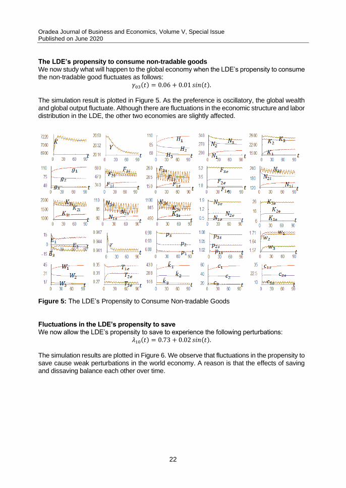
The LDE’s propensity to consume non-tradable goods We now study what will happen to the global economy when the LDE’s propensity to consume the non-tradable good fluctuates as follows:

𝛾03(𝑡) = 0.06 + 0.01 𝑠𝑖𝑛(𝑡). The simulation result is plotted in Figure 5. As the preference is oscillatory, the global wealth and global output fluctuate. Although there are fluctuations in the economic structure and labor distribution in the LDE, the other two economies are slightly affected.

Figure 5: The LDE’s Propensity to Consume Non-tradable Goods Fluctuations in the LDE’s propensity to save We now allow the LDE’s propensity to save to experience the following perturbations:

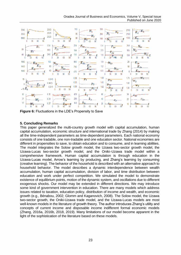
𝜆10(𝑡) = 0.73 + 0.02 𝑠𝑖𝑛(𝑡). The simulation results are plotted in Figure 6. We observe that fluctuations in the propensity to save cause weak perturbations in the world economy. A reason is that the effects of saving and dissaving balance each other over time.


23

Figure 6: Fluctuations in the LDE’s Propensity to Save 5. Concluding Remarks This paper generalized the multi-country growth model with capital accumulation, human capital accumulation, economic structure and international trade by Zhang (2014) by making all the time-independent parameters as time-dependent parameters. Each national economy consists of one tradable, one non-tradable and one education sector. National economies are different in propensities to save, to obtain education and to consume, and in learning abilities. The model integrates the Solow growth model, the Uzawa two-sector growth model, the Uzawa-Lucas two-sector growth model, and the Oniki–Uzawa trade model within a comprehensive framework. Human capital accumulation is through education in the Uzawa-Lucas model, Arrow’s learning by producing, and Zhang’s learning by consuming (creative learning). The behavior of the household is described with an alternative approach to household behavior. The model describes a dynamic interdependence between wealth accumulation, human capital accumulation, division of labor, and time distribution between education and work under perfect competition. We simulated the model to demonstrate existence of equilibrium points, motion of the dynamic system, and oscillations due to different exogenous shocks. Our model may be extended in different directions. We may introduce some kind of government intervention in education. There are many models which address issues related to taxation, education policy, distribution of income and wealth, and economic growth (e.g., Bénabou, 2002; Glomm and Kaganovich, 2008). The Solow model, the Uzawa two-sector growth, the Oniki-Uzawa trade model, and the Uzawa-Lucas models are most well-known models in the literature of growth theory. The author introduces Zhang’s utility and concepts of current income and disposable income indifferent formal economic models (Zhang, 2016a, 2016b, 2018, 2019). Many limitations of our model become apparent in the light of the sophistication of the literature based on these models.


24

Appendix: Proving the Lemma

We check the lemma. We omit time in expressions. From (2), we have: 𝑘𝑗𝑖 = 𝛼0𝑗 𝑘𝑗𝑠, (𝐴1)

where

𝛼0𝑗 ≡𝛼𝑗𝑖 𝛽𝑗𝑠

𝛼𝑗𝑠 𝛽𝑗𝑖

.

From (4) and (5), we determine 𝑝𝑗𝑠 as a unique function of 𝑘𝑗𝑖 as follows:

𝑝𝑗𝑠 =𝐴𝑗𝑖 𝛽𝑗𝑖 𝛼0𝑗

𝛼𝑗𝑠

𝐴𝑗𝑠 𝛽𝑗𝑠

𝑘𝑗𝑖

𝛼𝑗𝑖−𝛼𝑗𝑠.

By (5) and (7) 𝑝𝑗 are determined as unique functions of 𝑘𝑗𝑖 . From (2), we determine 𝑟 and 𝑤𝑞

as unique functions of 𝑘𝑗𝑖 . From (4), we 𝑘𝑗𝑖 as unique functions of 𝑘1𝑖 as follows:

𝑘𝑗𝑖 = (𝐴𝑗𝑖 𝛼𝑗𝑖

𝐴𝑗𝑖 𝛼1𝑖 𝑘𝑗𝑖

−𝛽𝑗𝑖− 𝛿1 + 𝛿𝑘

)

1/𝛽𝑗𝑖

, 𝐽 = 1, … , 𝐽. (𝐴3)

We have 𝑟, ,jsp 𝑝𝑗 , 𝑤𝑗 , 𝑘𝑗𝑠 and 𝑘𝑗𝑖 as unique functions of 𝑘1𝑖.

From (4) and (7), we obtain 𝑘𝑗𝑒 = 𝛼𝑗 𝑘𝑗𝑖 , (𝐴4)

where

𝛼𝑗 ≡𝛼𝑗𝑒 𝛽𝑗𝑖

𝛼𝑗𝑖 𝛽𝑗𝑒

.

We also determine 𝑘𝑗𝑒 as functions of 𝑘𝑗𝑖 . From (A4), (4) and (7), we obtain

𝑝𝑗 =𝐴𝑗𝑖 𝛼𝑗𝑖 𝛼𝑗

𝛽𝑗

𝐴𝑗𝑒 𝛼𝑗𝑒

𝑘𝑗𝑖

𝛽𝑗, (𝐴5)

where 𝛽𝑗 ≡ 𝛽𝑗𝑒 − 𝛽𝑗𝑖 . We solve 𝑝𝑗 as functions of 𝑘1𝑖 . By (12), we solve �̅�𝑗 and �̅�𝑗 as functions

of 𝑘1𝑖 and 𝐻𝑗 . From (7) and (16), we have:

𝑛𝑗𝑒 =𝑝0𝑗 𝑇𝑗𝑒

𝑁𝑗

. (𝐴6)

where 𝑝0𝑗 ≡ 𝛽𝑗𝑒𝑝𝑗𝑁𝑗/𝑤𝑗 . From (A6) and (2), we solve:

𝑛𝑗𝑖 ≡(𝑘𝑗 − 𝑘𝑗𝑠) 𝑁𝑗 + (𝑘𝑗𝑠 − 𝑘𝑗𝑒) 𝑝0𝑗 𝑇𝑗𝑒

(𝑘𝑗𝑖 − 𝑘𝑗𝑠) 𝑁𝑗

, 𝑛𝑗𝑖 ≡(𝑘𝑗𝑖 − 𝑘𝑗) 𝑁𝑗 + (𝑘𝑗𝑒 − 𝑘𝑗𝑖) 𝑝0𝑗 𝑇𝑗𝑒

(𝑘𝑗𝑖 − 𝑘𝑗𝑠) 𝑁𝑗

. (𝐴7)

From (17) and (13), we have

𝑛𝑗𝑠 =�̄�𝑗 𝛽𝑗𝑠 𝛾𝑗 �̄�𝑗

𝑤𝑗 𝑁𝑗

, (A8)

where we also use 𝑤𝑗 = 𝛽𝑗𝑠𝑝𝑗𝑠𝐹𝑗𝑠/𝑁𝑗𝑠. From (A7) and (A8), we solve:

(𝑘𝑗𝑖 − 𝑘𝑗)𝑁𝑗 + (𝑘𝑗𝑒 − 𝑘𝑗𝑖)𝑝0𝑗 𝑇𝑗𝑒 =(𝑘𝑗𝑖 − 𝑘𝑗𝑠)�̄�𝑗 𝛽𝑗𝑠 𝛾𝑗 �̄�𝑗

𝑤𝑗

. (A9)


25

Insert 𝑁𝑗 = 𝐻𝑗

𝑚𝑗𝑇𝑗�̄�𝑗 and 𝑇𝑗𝑒 = 𝜂𝑗 �̄�𝑗/�̄�𝑗 in (A9):

𝑇𝑗 =�̂�𝑗 �̄�𝑗

𝑘𝑗𝑖 − 𝑘𝑗

, (A10)

where

�̂�𝑗(𝑘1𝑖 , 𝐻𝑗) =1

𝐻𝑗

𝑚𝑗 �̄�𝑗

[(𝑘𝑗𝑖 − 𝑘𝑗𝑠)�̄�𝑗 𝛽𝑗𝑠 𝛾𝑗

𝑤𝑗

−(𝑘𝑗𝑒 − 𝑘𝑗𝑖)𝑝0𝑗 𝜂𝑗

�̄�𝑗

].

From (9) and in (13), we have: 𝑇𝑗 = 𝑇0 − �̃�𝑗 �̄�𝑗, (𝐴11)

where �̃�𝑗 ≡ 𝜂𝑗/�̄�𝑗 . From (A10) and (A11), we have 𝑘𝑗 = 𝑘𝑗𝑖 −�̂�𝑗 �̄�𝑗

𝑇0−�̃�𝑗 �̄�𝑗. (𝐴12)

From 𝐾𝑗 = 𝑘𝑗 𝑇𝑗 𝐻𝑗

𝑚𝑗 �̄�𝑗 , (A11) and (A12), we have: 𝐾𝑗 = ℎ𝑗1 �̅�𝑗 + ℎ𝑗2, (𝐴13)

where we use the definition of �̅�𝑗 and ℎ𝑗1 ≡ −(1 + 𝑟)(�̃�𝑗 𝑘𝑗𝑖 + �̂�𝑗)𝐻𝑗

𝑚𝑗 �̄�𝑗,

ℎ𝑗2 ≡ 𝑇0𝐻𝑗

𝑚𝑗 �̄�𝑗𝑘𝑗𝑖 − (�̃�𝑗 𝑘𝑗𝑖 + �̂�𝑗)𝐻

𝑗

𝑚𝑗 �̄�𝑗 𝑇0 �̄�𝑗 .

Insert (A13) in (18)

�̅�1 = Λ𝑘 ≡1

ℎ11 − �̄�1

(∑(�̄�𝑗 − ℎ𝑗1)�̅�𝑗

𝐽

𝑗=2

− ∑ ℎ𝑗2

𝐽

𝑗=1

).

All the variables can be expressed as functions of �̅�1𝑖 , (𝐻𝑗), {�̅�𝑗}, and 𝑡 by the procedure in

the Lemma. From the procedure in the Lemma and (15), we have:

�̇�𝑗 = Λ𝑗(�̅�1𝑖, (𝐻𝑗), {�̅�𝑗}, 𝑡). (𝐴15)

Here, we don’t provide explicit expressions of the functions as they are tedious. Substituting the definition of �̅�𝑗 into 𝑠𝑗 = 𝜆𝑗 �̅�𝑗 yields:

𝑠𝑗 = (1 + 𝑟) 𝜆𝑗 �̅�𝑗 + 𝜆𝑗 𝑇0 �̅�𝑗. (𝐴16)

Substituting (A16) into (14), we have:

�̇�1 = 𝜆1 𝑇0 �̅�1 − 𝑅 �̅�1 − �̇�1

𝑁1

�̅�1, (𝐴17)

�̇�𝑗 = Λ̅𝑗 ≡ 𝜆𝑗 𝑇0 �̅�𝑗 − (1 − 𝜆𝑗 − 𝜆𝑗 𝑟) �̅�𝑗 − �̇�𝑗

𝑁𝑗

�̅�𝑗, 𝑗 = 2, … 𝐽, (𝐴18)

in which 𝑅 ≡ 1 − 𝜆1 − 𝜆1 𝑟. Taking derivatives of equation (A14) with respect to 𝑡 yields:

�̇̅�1 =𝜕Λ𝑘

𝜕𝑘1𝑖

�̇�1𝑖 + ∑ Λ𝑗

𝜕Λ𝑘

𝜕𝐻𝑗

𝐽

𝑗=1

+ ∑ Λ̅𝑗

𝜕Λ𝑘

𝜕�̅�𝑗

𝐽

𝑗=2

+𝜕Λ𝑘

𝜕𝑡. (𝐴19)

where we use (A15) and (A18). Equaling the right-hand sizes of equations (A19) and (A17), we get:

�̇�1𝑖 = Λ̅1 ≡ [ 𝜆1 𝑇0 �̅�1 − 𝑅 Λ𝑘 − ∑ Λ𝑗

𝜕Λ𝑘

𝜕𝐻𝑗

𝐽

𝑗=1

− ∑ Λ̅𝑗

𝜕Λ𝑘

𝜕�̅�𝑗

𝐽

𝑗=2

−𝜕Λ𝑘

𝜕𝑡] (

𝜕Λ𝑘

𝜕𝑘1𝑖

)−1

. (𝐴20)

In summary, we proved the Lemma.


26

References Aghion, P. and Howitt, P., 1998. Endogenous Growth Theory. Mass., Cambridge: The MIT Press. Arcidiacono, P., Hotz, V.J., and Kang, S., 2012. Modelling College Major Choices Using Elicited Measures of Expectations and Counterfactuals. Journal of Economics, 166 (1), pp. 3–16. Arrow, K.J., 1962. The Economic Implications of Learning by Doing. Review of Economic Studies, 29, pp. 155-73. Attanasio, O.P. and Kaufmann, K.M., 2014. Education Choices and Returns to Schooling: Mothers' and Youths' Subjective Expectations and Their Role by Gender. Journal of Development Economics, 109, pp. 203–16. Azariadis, C., 1993. Intertemporal Macroeconomics. Oxford: Blackwell. Backus, D.K. and Smith, G.W., 1993. Consumption and Real Exchange Rates in Dynamic Economies with Non-Traded Goods. Journal of International Economics, 35, pp. 297–316. Barro, R.J., 2001. Human Capital and Growth. American Economic Review, Papers and Proceedings 91, pp. 12-17. Barro, R.J., 2013. Education and Economic Growth. Annals of Economics and Finance, 14 (2), pp. 301–28. Barro, R.J. and Lee, J.W., 2013. A New Data Set of Educational Attainment in the World, 1950–2010. Journal of Development Economics, 104 (C), pp. 184-98. Barro, R.J. and Sala-i-Martin, X., 1995. Economic Growth. New York: McGraw-Hill, Inc. Baxter, M., Jermann, U.J., and King, R.G., 1998. Nontraded Goods, Nontraded Factors, and International Non-Diversification. Journal of International Economics, 44, pp. 211–29. Bénabou, R., 2002. Tax and Education Policy in a Heterogeneous-Agent Economy: What levels of Redistrbution Maximize Growth and Efficiency? Econometrica, 70, pp. 481-517. Boozer, M. and Rouse, C., 2001. Intraschool Variation in Class Size: Patterns and Implications. Journal of Urban Economics, 50 (1), pp. 163–89. Bosworth, R., 2014. Class Size, Class Composition, and the Distribution of Student Achievement. Education Economics, 22, pp. 141-165. Bosworth, R. and Caliendo, F., 2007. Educational Production and Teacher Preferences. Economics of Education Review, 4, pp. 487–500. Burmeister, E. and Dobell, A.R., 1970, Mathematical Theories of Economic Growth. London: Collier Macmillan Publishers. Cachanosky, N., 2014. The Mises-Hayek Business Cycle Theory, Fiat Currencies and Open Economies. The Review of Austrian Economics, 3, pp. 281-99. Castelló-Climent, A. and Hidalgo-Cabrillana, A., 2012. The Role of Education Quality and Quantity in the Process of Economic Development. Economics of Education Review, 31 (4), pp. 391-409. Chatterjee, B. S. and Ravikumar, B., 1992. A Neoclassical Model of Seasonal Fluctuations. Journal of Monetary Economics, 29 (1), pp. 59–86. Chiarella, C. and Flaschel, P., 2000. The Dynamics of Keynesian Monetary Growth: Macro Foundations. Cambridge: Cambridge University Press Could, E.D., Moav, O., and Weinberg, B.A., 2001. Precautionary Demand for Education, Inequality, and Technological Progress. Journal of Economic Growth, 6, pp. 285-315. Dobbelsteen, S., Levin, J., and Oosterbeek, H., 2002. The Causal Effect of Class Size on Scholastic Achievement: Distinguishing the Pure Class Size Effect from the Effect of Changes in Class Composition. Oxford Bulletin of Economics and Statistics, 64 (1), pp. 17–38. Dominitz, J. and Manski, C.F., 1996. Eliciting Student Expectations of the Returns to Schooling. Journal of Human Resources, 31 (1), pp. 1–26.


27

Easterlin, R., 1981. Why Isn’t the Whole World Developed? Journal of Economic History, 41, pp. 1-19. Edwards, S., 1989. Temporary Terms of Trade Disturbances, the Real Exchange Rate and the Current Account. Economica, 56, pp. 343–57. Erosa, A., Koreshkova, T., and Restuccia, D., 2010. How Important Is Human Capital? A Quantitative Theory Assessment of World Income Inequality. The Review of Economic Studies, 77, pp. 1421-49. Fender, J. and Wang, P., 2003. Educational Policy in a Credit Constrained Economy with Skill Heterogeneity. International Economic Review, 44, pp. 939-64. Flaschel, P., Franke, R., and Semmler, W. 1997. Dynamic Macroeconomics. Cambridge, Mass: The MIT Press. Fleisher, B., Hu, Y.F., Li, H.Z., and Kim, S.H., 2011. Economic Transition, Higher Education and Worker Productivity in China. Journal of Development Economics, 94, pp. 86-94. Frenkel, J.A. and Razin, A., 1987. Fiscal Policy and the World Economy. MA., Cambridge: MIT Press. Gabaix, X., 2011. The Granular Origins of Aggregate Fluctuations. Econometrica ,79, pp. 733–772. Galor, O. and Moav, O., 2004. From Physical to Human Capital Accumulation: Inequality in the Process of Development. Review of Economic Studies, 71, pp. 1001-26. Galor, O. and Zeira, J., 1993. Income Distribution and Macroeconomics. Review of Economic Studies, 60, pp. 35-52. Gandolfo, G., 2005. Economic Dynamics. Berlin: Springer. Giovanni, J. Di., Levchenko, A., and Mejean, I., 2014. Firms, Destinations, and Aggregate Fluctuations. Econometrica, 82 (4), pp. 1303–1340. Glomm, G. and Kaganovich, M., 2008. Social Security, Public Education and the Growth-Inequality Relationship. European Economic Review 52, pp. 1009-1034. Grossman, G.M. and Helpman, E., 1991. Innovation and Growth in the Global Economy. Cambridge, Mass.: The MIT Press. Hanushek, E. and Kimko, D., 2000. Schooling, Labor-Force Quality and the Growth of Nations. American Economic Review, 90, pp. 1194-1204. Hanushek, E.A., Leung, C.K.Y., and Yilmaz, K., 2014. Borrowing Constraints, College Aid, and Intergenerational Mobility. Journal of Human Capital, 8 (1), pp. 1-41. Hanushek E.A. and Woessmann, L., 2008. The Role of Cognitive Skills in Economic Development. Journal of Economic Literature, 46 (3), pp. 607-668. Hohberger, S., Vogel, L., and Herz, B., 2014. Budgetary-Neutral Fiscal Policy Rules and External Adjustment. Open Economies Review, 25, pp. 909-936. Ikeda, S. and Ono, Y., 1992. Macroeconomic Dynamics in a Multi-Country Economy - A Dynamic Optimization Approach. International Economic Review, 33, pp. 629-644. Jensen, R., 2010. The (Perceived) Returns to Education and the Demand for Schooling. Quarterly Journal of Economics, 125 (2), pp. 515–48. Kaarsen, N., 2014. Cross-country Differences in the Quality of Schooling. Journal of Development Economics, 107, pp. 215–224. Krueger, A.B. and Lindahl, M., 2001. Education for Growth: Why and for Whom. Journal of Economic Literature, 39, pp. 1101-1136. Krueger, A.B. and Whitmore. D.M., 2001. The Effect of Attending a Small Class in the Early Grades on College-Test Taking and Middle School Test Results: Evidence from Project STAR. Economic Journal, 111 (468), pp. 1–28. Lazear, E.P., 2001. Educational production. Quarterly Journal of Economics 116 (3) 777–803. Lorenz, H.W., 1993. Nonlinear Dynamic Economics and Chaotic Motion. Berlin: Springer-Verlag.


28

Lucas, R.E., 1977. Understanding Business Cycles. Carnegie-Rochester Conference Series on Public Policy, 5, pp. 7-29. Lucas, R.E., 1988. On the Mechanics of Economic Development. Journal of Monetary Economics, 22, pp. 3-42. Maasoumi, E., Millimet, D.L. and V. Rangaprasad, D.M., 2005. Class Size and Educational Policy: Who Benefits from Smaller Classes? Econometric Reviews, 24 (4), pp. 333–68. Maoz, Y.D. and Moav, O., 1999. Intergenerational Mobility and the Process of Development. Economic Journal, 109, pp. 677-97. Mendoza, E.G., 1995. The Terms of Trade, the Real Exchange Rate, and Economic Fluctuations. International Economic Review, 36, pp. 101–137. Mincer, J., 1974. Schooling, Experience and Earnings. New York: Columbia University Press. Nishimura, K. and Shimomura, K., 2002. Trade and Indeterminacy in a Dynamic General Equilibrium Model. Journal of Economic Theory, 105, pp. 244-260. Nolte, D.D., 2015. Introduction to Modern Dynamics: Chaos, Networks, Space and Time. London: Oxford University Press Oniki, H. and Uzawa, H., 1965. Patterns of Trade and Investment in a Dynamic Model of International Trade. Review of Economic Studies, 32, pp. 15-38. Pesenti, P., van Wincoop, E., 2002. Can Nontradables Generate Substantial Home Bias? Journal of Money, Credit and Banking, 34, pp. 25–50. Puu, T., 2011. Nonlinear Economic Dynamics. Berlin: Springer. Raleva, S., 2013. Structural Sources and Characteristics of the Inflation in Bulgaria (1992-2010). Economic Studies, 1, pp. 41-71. Rogoff, K., 2002. The Purchasing Power Parity Puzzle. Journal of Economic Literature, 34, pp. 647–668. Romer, P.M., 1986. Increasing Returns and Long-Run Growth. Journal of Political Economy, 94, pp. 1002-1037. Shone, R., 2002. Economic Dynamics – Phase Diagrams and Their Economic Application. Cambridge: Cambridge University Press. Solow, R., 1956. A Contribution to the Theory of Growth. Quarterly Journal of Economics, 70, pp. 65-94. Sorger, G., 2002. On the Multi-Country Version of the Solow-Swan Model. The Japanese Economic Review, 54, pp. 146-64. Stella, A., 2015. Firm Dynamics and the Origins of Aggregate Fluctuations. Journal of Economic Dynamics and Control, 55 (C), pp. 71-88. Stinebrickner, T. and Stinebrickner, R., 2012. Learning about Academic Ability and the College Drop-Out Decision. Journal of Labor Economics, 30 (4), pp. 707–748. Stockman, A.C. and Dellas, H., 1989. International Portfolio Nondiversification and Exchange Rate Variability. Journal of International Economics, 26, pp. 271-289. Stockman, A.C. and Tesar, L.L., 1995. Tastes and Technology in a Two-country Model of the Business Cycle: Explaining International Comovements. American Economic Review, 85, pp. 168–185. Stulz, R. M., 1987. An Equilibrium Model of Exchange Rate Determination and Asset Pricing with Nontraded Goods and Imperfect Information. Journal of Political Economy, 95, pp. 1024-1040. Tilak, J.B.C., 1989. Education and Its Relation to Economic Growth, Poverty and Income Distribution: Past Evidence and Future Analysis. Washington: World Bank. Tselios, V., 2008. Income and Educational Inequalities in the Regions of the European Union: Geographically Spillovers under Welfare State Restrictions. Papers in Regional Science, 87, pp. 403-430. Urquiola, M. and Verhoogen, E., 2009. Class-size Caps, Sorting, and the Regression Discontinuity Design. American Economic Review, 99 (1), pp. 179–215.

http://www.amazon.com/Nonlinear-Economic-Dynamics-T%C3%B6nu-Puu/dp/3642645496/ref=sr_1_16?s=books&ie=UTF8&qid=1429663484&sr=1-16&keywords=nonlinear+dynamics%2C+economic

http://www.amazon.com/Nonlinear-Economic-Dynamics-T%C3%B6nu-Puu/dp/3642645496/ref=sr_1_16?s=books&ie=UTF8&qid=1429663484&sr=1-16&keywords=nonlinear+dynamics%2C+economic


29

Uzawa, H., 1965. Optimal Technical Change in an Aggregative Model of Economic Growth. International Economic Review, 6, pp. 18-31. Wossmann, L. and West, M., 2006. Class-size Effects in School Systems around the World: Evidence from Between-Grade Variation in TIMSS. European Economic Review, 50 (3), pp. 695–736. Zhang, W.B., 1991. Synergetic Economics. Heidelberg: Springer-Verlag. Zhang, W.B., 1993. Woman’s Labor Participation and Economic Growth - Creativity, Knowledge Utilization and Family Preference. Economics Letters, 42, pp. 105-110. Zhang, W.B., 2005. Differential Equations, Bifurcations, and Chaos in Economics. Singapore: World Scientific. Zhang, W.B., 2006. Discrete Dynamical Systems, Bifurcations and Chaos in Economics. Amsterdam: Elsevier. Zhang, W.B., 2007. Economic Growth with Learning by Producing, Learning by Education, and Learning by Consuming. Interdisciplinary Description of Complex Systems, 5, pp. 21-38. Zhang, W.B., 2013. Income and Wealth Distribution with Physical and Human Capital Accumulation: Extending the Uzawa-Lucas Model to a Heterogeneous Households Economy. Latin American Journal of Economics, 50 (2), pp. 257-287. Zhang, W.B., 2014. Tradable, Non-tradable and Education Sectors in a Multi-Country Economic Growth Model with Endogenous Wealth and Human Capital. Economic Research Guardian, 4 (2), pp. 65-85. Zhang, W.B., 2016a. Population Growth and Preference Change in a Generalized Solow Growth Model with Gender Time Distributions. Oradea Journal of Business and Economics, 1 (2), pp. 7-30. Zhang, W.B., 2016b. Fashion with Snobs and Bandwagoners in a Three-Type Households and Three-Sector Neoclassical Growth Model. The Mexican Journal of Economics and Finance, 11 (2), pp. 1-19. Zhang, W.B., 2018. A Growth Theory Based on Walrasian General Equilibrium, Solow-Uzawa Growth, and Heckscher-Ohlin Trade Theories. Interdisciplinary Description of Complex Systems - Scientific Journal, 16 (3-B), pp. 452-464. Zhang, W.B., 2019. Money and Price Dynamics under the Gold Standard in the One-Sector Neoclassical Growth Model. Lecturas de Economía, 90, pp. 45-69. Zhao, Y., Guo, S., and Liu, X.F., 2014. Trading Frictions and Consumption-output Comovement. Journal of Macroeconomics, 42, pp. 229-240. Zhu, R., 2011. Individual Heterogeneity in Returns to Education in Urban China during 1995-2002. Economics Letters, 113, pp. 84-87. Bio-note: Zhang Wei-Bin, PhD (Umeå, Sweden), is Professor in APU since 2000. He was graduated in 1982 from Department of Geography, Beijing University. He got Master Degree and completed Ph.D course at Department of Civil Engineering, Kyoto University in 1987. He completed his dissertation on economic growth theory in June, 1989. Since then he researched at the Swedish Institute for Futures Studies in Stockholm for 10 years. His main research fields are nonlinear economic dynamics (synergetic economics), economic theory, ancient Confucianism, and economic development and modernization of Chinese societies. He single-authorized 300 academic articles (210 in international peer-reviewed journals), 22 academic books in English. He is editorial board members of 14 peer-review international journals. Prof. Zhang is the editor of Encyclopedia of Mathematical Models in Economics (in two volumes) as a part of the unprecedented global effort, The Encyclopedias of Life Support Systems, organized by The UNESCO.

Date post:	08-Dec-2021
Category:	Documents
Upload:	others
View:	1 times
Download:	0 times

GLOBAL DEVELOPMENT, TRADE, HUMAN CAPITAL, AND …

Documents