Global Dynamics of an SEIRS Epidemic Model with … Dynamics of an SEIRS Epidemic Model with...

Global Dynamics of an SEIRS Epidemic Model with ConstantImmigration and Immunity

Li juan ZhangInstitute of disaster prevention

Basic Course DepartmentSanhe, Hebei 065201

P. R. [email protected]

Yingqiu Li Qingqing Ren Zhenxiang HuoInstitute of disaster prevention

Basic Course DepartmentSanhe, Hebei 065201

P. R. CHINA

Abstract: An SEIRS model for disease transmission that includes immigration of the infective, susceptible, ex-posed, and recovered has been constructed and analyzed. For the reason that the immunity of the recovered istemporary, a proportion δ1 of recovered will come back to susceptible. We also consider vaccine injection to thesusceptible with a proportion c. The model also incorporates a population size dependent contact rate and a disease-related death. As the infected fraction cannot be eliminated from the population, this kind of model has only oneunique endemic equilibrium that is globally asymptotically stable. In a special case where the new members ofimmigration are all susceptible, the model shows a threshold phenomenon. In order to prove the global asymptot-ical stability of the endemic equilibrium, we change our system to a three-dimensional asymptotical autonomoussystem with limit equation. Finally, we discussed syphilis as a case to predict the development in China. Computersimulation shows that the model can reflect the dynamic and immigration behaviour for disease transmission.

Key–Words: SEIRS model, population size dependent contact rate, syphilis, compound matrix

1 IntroductionThe incidence of a disease is the number of new casesper unit time, and it plays an important role in thestudy of mathematical epidemiology. Thieme andCastillo-Chavez [1] argued that the general form of apopulation-size-dependent incidence should be writ-

ten as βλ(N)SI

N, where S is the number of suscepti-

ble at time t, I the number of infective at time t, andN the total population size at time t, then S+ I ≤ N ,β is the probability per unit time of transmitting a dis-ease between two individuals in contact. And λ(N) isthe probability for an individual to take part in a con-tact. In many articles λ(N) is also called the contactrate, βλ(N) , C(N) which is the average numberof adequate contacts of an individual per unit time issaid to be an adequate contact rate. An adequate con-tact is a contact which is sufficient for transmission ofthe infection from an infective to a susceptible. Manycontact rate forms are used in the incidence term indeterministic epidemic models described by differen-tial equation. For example the standard incidence λSI

Nstarts with the assumption that adequate contact rateis constant λ. The bilinear incidence λSI = βN S

N Iimplies that the adequate contact rate is βN that islinearly proportional to the total population size N .This would be realistic when the total population size

N is not too large because the number of adequatecontacts made by an individual per unit time shouldincrease as the total population size N increases. Onthe contrary, if population size is quite large, becausethe number of adequate contacts made by an infectiveper unit time should be limited, or grows less rapidlyasN increases, the linear contact rate βN is not avail-able and the constant adequate contact rate λ may bemore realistic. Hence the two above-mentioned ade-quate contact rates are actually two extreme cases forthe total population size N being very small and verylarge.

Many expressions have also been used for the in-cidence term. Anderson [2] argued that if C(N) =λN δ is an appropriate contact rate, then the incidenceis C(N) = λN δSI/N . The data in Anderson arti-cle [2] for human diseases in communities with pop-ulation sizes from 1000 to 400000 imply that δ is be-tween 0.03 and 0.07.That also shows that the inci-dence give by C(N)SI/N with a contact rate suchas C(N) = λN0.05 would be even better.

In analogy to Hollings [3] derivation of predater’sfunctional response to the amount of prey, the con-tact function C(N) should be βaN

1+bN . Heesterbeek andMetz [4] derived an effective contact rate of the formC(N) = βbN

1+bN+√1+2bN

,which is modelling the for-mation of the short-time social complexes.

WSEAS TRANSACTIONS on MATHEMATICS Li Juan Zhang, Yingqiu Li, Qingqing Ren, Zhenxiang Huo

E-ISSN: 2224-2880 630 Issue 5, Volume 12, May 2013

All above-mentioned adequate contact rate formssatisfy the following two assumptions:

(H1) C(N) is a nonnegative continuous functionas N ≥ 0 and is continuous differential as N > 0;

(H2) D(N) = C(N)/N is a non-increasing con-tinuously differentiable function asN > 0, D(0) = 0and C ′(N) + |D′(N)| = 0.

Many authors have done researches on SEIRmodels of epidemics transmission recently. Green-halgh [4] considered SEIR models that incorporatedensity dependence in the death rate. Cooke and vanden Driessche [5] introduced and studied the SEIRSmodels with two delays. Recently, Greenhalgh [6]studied Hopf bifurcations in models of the SEIRStype, with density- dependent contact rate and deathrate. Li and Muldowney [7] and Lietal [8], studiedglobal dynamics of the SEIR models with a nonlin-ear incidence rate and with a standard incidence, re-spectively. Li et al. [9] analyzed the global dynam-ics of an SEIR model with vertical transmission anda bilinear incidence. Research on epidemic modelsof SEIR or SEIRS types with the general population-size-dependent adequate contact rate C(N) satisfyingthe assumptions (H1) and (H2) are scarce in the pub-lished reports. Zhang [10] has studied an SEIR modelwith population size dependent contact rate and newflow of immigration, but has not considered the failureof immunity and the vaccination. But it is well knownthat they are very important in reality.

In this manuscript, we construct and study theSEIRS epidemic model with a general contact rate andimmigration of distinct compartments. Especially, toestablish the global stability of the endemic equilib-rium, we reduced the model to a three-dimensionalasymptotical autonomous differential system with alimit system. C(N)/I is a general population-size-dependent function satisfying the assumptions (H1)(H2). We assume a constant proportion of new mem-bers into the population per unit time, of which a frac-tion q is exposed, a fraction p is infective, and a frac-tion b is recovered. So the fraction 1−p−q−b is sus-ceptible, where p, q, b are nonnegative constants with0 ≤ p+q+b ≤ 1. Assume that natural deaths occur ata rate proportional to the population size N . Then thenatural death rate term is µN , µ is the natural deathrate constant. Under our assumptions, the infectioncannot be eliminated because there is a constant newinfected individuals moving in, when 1 − q − p > 0.In order to eradicate the disease, it would be neces-sary to isolate the fraction of arriving infected individ-uals. Our model has some features in common withmodels that include vertical transmission, but verticaltransmission models normally include a new infectedproportional, which are already in the population andthus may have a disease-free equilibrium [11,12]. We

also make some simulation with the syphilis. Withour conclusion, we can make some prediction. Thiscan be used to some disease control department andso on.

2 Problem Formulation2.1 Model FormulationThe total population sizeN(t) is divided into four dis-tinct epidemic subclasses (compartments) of individu-als which are susceptible, exposed, infectious, and re-covered (with temporary immunity), with the denotedS(t), E(t), I(t), and R(t) respectively. q, p and b areall nonnegative constant, and 0 ≤ p + q + b ≤ 1.The parameters µ, ε, γ are all positive constants. αis a nonnegative constant and represents the death ratebecause of disease (the disease-related death rate), weassume it is small. µ is the rate constant for naturaldeath, γ is the rate constant for recovery, and ε is therate constant at which the exposed individuals becomeinfective, so that 1

ε is the mean latent period. The re-covered individuals are assumed to acquire temporaryimmunity, so there is transfer from class R back toclass S with a proportion δ1. The positive constantA is the constant recruitment rate into the population,so that A/µ represents a carrying capacity, or maxi-mum possible population size, rather than the popu-lation size N . C(N) satisfying the assumptions (H1)and (H2) is the adequate contact rate. Then the SEIRSmodel with the adequate contact rate and immigrationof different compartment individuals is derived on thebasis of the basic assumptions. By using the trans-fer diagram, it is described by the following system ofdifferential equations

S′ = (1− p− q − b)A− βλ(N)S

NI

− µS + δ1R− cS

E′ = qA+ βλ(N)S

NI − µE − εE

I ′ = pA+ εE − µI − αI − γI (1)R′ = bA+ γI − µR+ cS −Rδ1N(t) = S(t) + E(t) + I(t) +R(t).

We study (1) in the closed set:

Γ = {(S,E, I,R) ∈ R4+ : 0 ≤ S + E + I

+R = N ≤ A/µ}

R+4 denotes the nonnegative cone of R4, including its

lower dimensional faces. It can be verified that Γ ispositively invariant with respect to (1). ∂Γ, Γ denotethe boundary and the interior of Γ respectively.



The continuity of the right side of (1) on N > 0implies that solutions exist in Γ and solutions remainin Γ, they are continuous for all t > 0 (see [13]).

If D(N) =βλ(N)

N=

C(N)

N, D(N) ∈ C ′[0,

A

µ],

then the right side of (1) is globally Lipschitz in Γso that the initial value problem has a unique solu-tion for all t ≥ 0 that depends continuously on thedata. IfD′(0) is bounded, thenD′(N) is still boundedon [0, A/µ]. Then in the interior of the region Γ, theright side of (1) is locally Lipschitz, as a Lipschitzconstant exists for every closed bounded subset of theinterior of Γ. Thus for any point in the interior of Γ,the initial value problem has a unique solution for allt ≥ 0. If 0 < p + q + b < 1, the solutions starting atpoints on the boundary of Γ enter the interior of Γ. Ifp+q+b = 0, solutions starting on the S-axis approach

P0 =( A(µ+ δ1)

µ(µ+ δ1 + c), 0, 0,

Ac

µ(µ+ δ1 + c)

), but all

the other solutions starting at points on the boundaryof Γ enter the interior of Γ .If p + q = 1 − b, for allsolutions starting at points on the boundary of Γ, theyenter the interior of Γ or stay on ∂Γ. So the initialvalue problem is well posed in a close set Γ.

2.2 EquilibriumThe equilibrium of system (1) can be found by settingthe right sides of the four equations of (1) equal tozero, giving the algebraic system

(1− p− b− q)A− SID(N)− µS+δ1R− cS = 0

qA+D(N)SI = (µ+ ε)E (2)pA+ εE = (µ+ α+ γ)I

bA+ γI = µR− cS + δ1R.

Adding all equations in (2), we obtain

I =1

α(A− µN) (3)

Let δ = µ+ α+ γ, ω = µ+ ε then R and E canbe expressed in terms of N :

R =bA

µ+ δ1+γ(A− µN)

α(µ+ δ1)+

αc(1− q − b− p)A(µ+ δ1)(αµ+D(N)A−D(N)µN + αδ1 + αc)

(4)

E =δ

εI − pA

ε(A− µN)− pA

ε

S =α(1− p− b− q)A

αµ+D(N)(A− µN) + αδ1 + αc(5)

Substituting (4) and (5) into the second equation in(2),we have

1

α(A− µN)[D(N)

α(1− p− b− q)Aαµ+D(N)(A− µN) + αδ1 + αc

− (µ+ ε)δ

ε] +

pA(µ+ ε)

ε+ qA = 0 (6)

The existence and number of equilibrium corre-spond to those of the roots of the equation (6) in the

interval [0,A

µ].

R0 = βλ(A/µ)ε

ε+ µ

1

µ+ γ + α=εC(A/µ)

δω(7)

Theorem 1 Suppose p + q + b = 0 or new membersof immigration are all susceptible.

The point

P0 =

(A(µ+ δ1)

µ(µ+ δ1 + c), 0, 0,

Ac

µ(µ+ δ1 + c)

)is the disease-free equilibrium of the system (1). It isstable when R0 ≤ 1 and unstable when R0 > 1

1. When R0 < 1, the solutions of the system (1)starting sufficiently close to P0 in Γ move away fromP0 except those starting on the invariant S-axis whichapproach P0 along the axis.

2. When R0 > 1 system (1) has a unique interior(endemic) equilibrium and its coordinates satisfy (3)-(5)if and only if R0is between µ

µ+δ1+candC(A/µ)α .

Proof. When p + q + b = 0, that is p = q = b = 0,the equation (6) becomes:

G(N) = [D(N)αA

α(µ+ δ1 + c) +D(N)(A− µN)

− (µ+ ε)δ

ε]1

α(A− µN)

= 0.

We can see that either A − µN = 0, then I = 0, andwe can deduce

E = 0, I = 0, R =cA

µ(µ+ c+ δ1), S =

Aµ+Aδ1µ(µ+ c+ δ1)

.

WhenR0 ≤ 1, we setL = εE+ωI , then its derivativealong the solutions of (1) is

L′ = δωI(R0S

N

C(N)

C(A/µ)− 1) ≤ 0.

That implies that all paths in Γ approach the largestpositively invariant subset of the set M where L′ = 0.



The reason is the Lyapnuov-Lasell theorem [18]. Mis the set where I = 0. At the same time E = 0.

S′ =(A+ δ1R)− (µ+ c)s

S =A+ δ1R

µ+ c+ [S(0)− A+ δ1R

µ+ c]e(−µ−c)S

S →A+ δ1R

µ+ c

We can conclude that all solutions of (1) will approachthe disease-free equilibrium.

When R0 > 1 then L′ can be written as:

L′ = δωI(R0S

A/µ

D(N)

D(A/µ)− 1).

So L′ > 0 for S which is sufficiently close to A/µ,except the invariant S-axis.

Solutions starting sufficiently close to P0 moveaway neighbourhood of P0, except those starting onthe S-axis which approach P0. From the assumptions(H1) and (H2), the function G(N) is decreasing, sothat the equation G(N) = 0 has at most one uniqueroot. We let

F (N)

= D(N) αAαµ+D(N)(A−µN)+αδ1+αc −

(µ+ε)δε

= AαC(N)Nα(µ+δ1+c)+C(N)(A−µN) −

1R0

C(A/µ)α

limN→0

F (N) = 1− 1R0

C(A/µ)α

limN→A/µ

F (N) = C(A/µ)

(µ

µ+δ1+c −1R0

).

If and only if R0 is between µµ+δ1+c and C(A/µ)/α,

that is forµ

µ+ δ1 + c< R0 < C(A/µ)/α

orC(A/µ)/α < R0 <

µ

µ+ δ1 + c,

equation (6) has only one positive root in the inter-val N1 ∈ (0, A/µ). That is the system has one en-demic equilibrium P1 = (S1, E1, I1, R1) except dis-ease equilibrium P0, and it satisfies:

S1 =α(1− p− q − b)A

αµ+D(N1)(A− µN1) + αδ1 + αc

I1 =1

α(A− µN1)

E1 =δ

αε(A− µN1)−

pA

ε

R1 =αc(1− p− q − b)A

(µ+ δ1)(αµ+D(N1)(A− µN1) + αδ1 + αc)

+bA

µ+ δ1+γ(A− µN1)

α(µ+ δ1)

is coordinates of P1 satisfy(3)-(5)when p = 0, q =0, b = 0, where N = N1.

Theorem 2 When p + q + b = 1, that is all of newmembers of immigration are not susceptible, system(1) has a unique boundary equilibrium,

P2 =

(0,

qA

µ+ ε,pA+ qAε/µ+ ε

µ+ α+ γ,

bA

µ+ δ1

+pAγ

δ(µ+ δ1)+

qAωγ

ωδ(µ+ δ1)

)and it is globally asymptotically stable.

Proof. Let 0 < p+q < 1−b in system (1), it is easy tosee that P2is the unique equilibrium of the system(1).The global asymptotical stability of the point P2 canbe proved by using the function L = S. ⊓⊔

Theorem 3 When 0 < p+ q < 1− b system (1) onlyhas equilibrium P ∗ = (S∗, E∗, I∗, R∗) and P ∗ is inthe feasible region of Γ.

Proof. It is easy to see that system (1) has no disease-free equilibrium, the equation (6) becomes

1

α(A− µN)[D(N)

α(1− p− q − b)Aαµ+D(N)(A− µN) + αδ1 + αc

− (µ+ ε)δ

ε] +

pA(µ+ ε)

ε+ qA = 0

to simplify we can see

G(N) =1α(A− µN)[ C(N)(1−p−q−b)Aα

(A−µN)C(N)+Nα(µ+δ1+c) −ωδε ]

+pAωε + qA = 0

From the assumptions (H1)-(H2), the functionG(N) is decreasing, so the equation has at most aunique root. And we have

limN→0

G(N) =(1− p− q − b)A− ωδA

αε+pAω

ε

=A

εα[µ(α− ε− c)− εγ − εαb] < 0,

limµ→A/µ

G(N) =pAω

ε+ qA > 0.

So the equation G(N) = 0 exists only one posi-tive root N∗ in (0, A/µ) .



Now we can find the only equilibrium P ∗ =(S∗, E∗, I∗, R∗) satisfying

I∗ =1

α(A− µN∗)

S∗ =α(1− p− q − b)A

αµ+D(N∗)(A− µN∗) + αδ1 + αc

E∗ =δ

αε(A− µN∗)− pA

ε

R∗ =αc(1− p− q − b)A

(µ+ δ1)(αµ+D(N∗)A−D(N∗)µN∗ + αδ1 + αc)

+γ(A− µN∗)

α(µ+ δ1)+

bA

µ+ δ1

2.3 Global stability of the EquilibriumIn this section, we establish that all solutions of (1) inthe interior of Γ converge to P ∗ if 0 < p+ q < 1− band to P1 if p + q + b = 0 and if R0is between

µ

µ+ δ1 + cand C(A/µ)/α respectively. For this pur-

pose, we first introduce the change of variable thatcan reduce the four-dimensional autonomous system(1) into a three-dimensional asymptotical autonomoussystem with a limit system, then prove that the equilib-rium of this limit system corresponding to P1 and P ∗

are globally asymptotically stable, by using the geo-metric approach to global stability problems in Li andMuldowney [14]. This implies the main conclusion inCorollary 3.1 of the third section.

For system (1), let δ1 = 0 then the equation canbe:

S′ =(1− p− q − b)A− βλ(N)S

NI − µS − cS

E′ =qA+ βλ(N)S

NI − µE − εE (8)

I ′ =pA+ εE − µI − αI − γI

N,R can be obtained from N ′ = A − µN − αI andR = N − S − E − I . The feasible region of (8) isT = {(S,E, I) ∈ R3

+ : 0 ≤ S + E + I ≤ A/µ} ispositively invariant with respect to (8), where R3

+ de-notes the nonnegative cone of R3, including its lowerdimensional faces. Thus system (8)is bounded.

Lemma 1 Suppose p+ q + b = 0

1 If R0 ≤ 1, Q0 =( A(µ+ δ1)

µ(µ+ δ1 + c), 0, 0

)is the only

equilibrium in T and it is globally asymptoticallystable. If R0 > 1, Q0 becomes unstable, whereasQ1 = (S1, E1, I1) is corresponding to the equi-librium P1 of system (1), and emerges as a unique

equilibrium in the interior of T , whereR0 is definedby (7)

I1 =1

α(A− µN1)

E1 =δ

αε(A− µN1)−

pA

ε

S1 =α(1− p− q − b)A

αµ+D(N1)(A− µN1) + αδ1 + αc

R1 =bA

µ+ δ1+γ(A− µN1)

α(µ+ δ1)

+αc(1− p− q − b)A

(µ+ δ1)(αµ+D(N1)(A− µN1) + αδ1 + αc)

N1 is the unique root of the equation G(N) = 0 .

2 When R0 > 1 the solutions of system (7) startingsufficiently close toQ0 in T move away fromQ0 ex-cept that starting on the invariant S-axis approachQ0 along this axis.

Lemma 2 When 0 < p + q < 1 − b, the system (7)has the only equilibrium Q∗ = (S∗, E∗, I∗), whichis corresponding to the equilibrium P ∗ of system (1),and Q∗ is in the interior of the feasible region of T ,where

I∗ =1

α(A− µN∗)E∗

E∗ =δ

αε(A− µN∗)− pA

ε

S∗ =α(1− p− q − b)A

αµ+D(N∗)(A− µN∗) + αδ1 + αc

Lemma 3 The system (8) is uniformly persistent ifeither p + q + b = 0, R0 between

µ

µ+ δ1 + cand

C(A/µ)/α or 0 < p+ q < 1− b holds.

Proof. If 0 < p + q < 1 − b, it is easy to see that thevector field of system (8) is transversal to the bound-ary of T on all its faces.

If p+ q+ b = 0, the vector field of the system (8)is transversal to boundary of T on all its faces exceptthe S-axis, which is invariant with respect to (8). On

the S-axis the equation of S :dS

dt= A − µS − cS,

implies

S(t)→ A

µ+ cas t→ +∞

If p+ q+ b = 0, Q0 is a only ω-limit point on theboundary of T .

The system is said to be uniformly persistent( [15, 16]) if there exists constancy c with 0 <



c < 1 such that any solution (S(t), E(t), I(t))

with initial data (S(0), E(0), I(0)) ∈ T satisfieslimt→∞

inf |(S(t), E(t), I(t))| ≥ c.The conclusion of the lemma follows from The-

orem 4.3 in [17], as the maximal invariant set on theboundary ∂T of T is an empty set when 0 < p+ q <1− b and the singleton {Q0} and Q0 is isolated whenp + q + b = 0 and R0 between

µ

µ+ δ1 + cand

C(A/µ)/α, thus the hypothesis (H) of [17] holdsfor(8). The conclusion for uniform persistence in The-orem 4.3 of [17] is equivalent to Q0 being unstablewhen p + q + b = 0 and R0 > 1. Thus, system(8)isuniformly persistent in T .

The main aim of this section is to prove the fol-lowing Theorem.

Theorem 4 1) When p + q + b = 0 and R0 betweenµ

µ+ δ1 + candC(A/µ)/α, the unique endemic equi-

librium P1 of system (1)is globally asymptotically sta-ble in the interior of Γ. Moreover, P1 attracts all tra-jectories in Γ except those on the invariant S-axis thatconverge to P0 along this axis.

2) When 0 < p + q < 1 − b, the unique endemicequilibrium P ∗ of system (1)is globally asymptoticallystable in the interior of Γ.

By inspecting the vector field given by (1), we seethat if 0 < p+ q < 1− b, all trajectories starting fromthe boundary ∂Γ of Γ enter the interior Γ of Γ.

When p + q + b = 0, they do except those so-lutions on the S-axis that converge to P0, along thisinvariant axis. Thus we need only to prove that Γ isthe attractive region of P ∗ when 0 < p + q < 1 − band P1 when p+ q + b = 0 respectively.

For the results in Theorem 1 and Theorem 3,we utilize a geometric approach to the global stabil-ity problem developed in Li and Muldowney [19]andSmith [18]. Here we apply the theory, in particularTheorem A.2 in the appendix, to prove the followingtheorem. In addition, it is remarked in [18], under theassumptions of theorem A.2 in the appendix, the con-dition q2 < 0 also implies the local stability of theequilibrium x, as assuming the contrary, x is both thealpha and omega limit of a homo-clinic orbit that isruled out by the condition q2 < 0.

From Lemma 1 we can make the following con-clusions.

Lemma 4 1) If 0 < p + q < 1 − b, Q∗ is globallyasymptotically stable.

2) When p + q + b = 0 and R0is betweenµ

µ+ δ1 + cand C(A/µ)/α, Q1 is globally asymptot-

ically stable.

Proof. By Lemma 3, there exists a compact set K inthe interior of Γ that is absorbing(8). Thus, in theclosed set T the system (8) satisfies the assumptionsH3, H4, H5 in appendix [17]. Let x = (S,E, I) andf(X) denote the vector field of (8). The Jacobian ma-

trix J =∂f

∂xAssociated with a general solution of (8) is:

J =

a11 a12 a13a21 a22 a230 ε −δ

Where we have:

a11 =−D(N)I − ISD′(N)− c− µa12 =− SID′(N)

a13 =−D(N)S −D′(N)SI

a21 =D(N)I + ISD′(N)

a22 =D′(N)SI − µ− ε

a23 =D(N)S +D′(N)SI

The second compound matrix J [2] of J can be cal-culated as follows:

J [2] =

b11 b12 b13ε b22 b230 b32 b33

where

b11 =a11 + a22 = −D(N)I − c− 2µ− εb22 =a11 + a33 = −δ − c− µ−D(N)I − ISD′(N)

b33 =a22 + a33 = −δ − µ− ε+D′(N)SI

b12 =a23 b13 = −a13 b23 = a12 b32 = a21

The proof of the theorem consists of choosing asuitable vector norm | · | in R3 and a 3 × 3 matrix-valued function A(x), such that the quantity q2 de-fined by (A.2) in the appendix is negative. We set Aas the following diagonal matrix.

A(S,E, I) = diag(1,E

I,E

I) (9)

Then A is C1 and non-singular in the interior of T .Thus

AfA− =diag

(0,I

E

(EI

)f,I

E

(EI

)f

)=diag

(0,E′

E− I ′

I,E′

E− I ′

I

)



Therefore the matrixB = AfA−1+AJ [2]A−1 can be

written in the block form

B =

[B11 B12

B21 B12

]With

B11 =−D(N)I − c− 2µ− ε

B21 =

[EεI0

]

B12 =I

E

(D(N)S +D′(N)SI

) [1 1

]B22 =

[c11 −SID′(N)

D(N)I + ISD′(N) c22

]c11 =

E′

E− I ′

I− µ− δ − c−D(N)I − ISD′(N)

c22 =E′

E− I ′

I− µ− δ − ε+D′(N)IS

Choosing the vector norm | · | in R

[32

]∼= R3 as

|(u, v, w)| = sup{|u|, |v|+ |w|}The Lozinskii measure ρ(B) with respect to | · |

can be estimated as follows (see [18]): ρ(B) ≤sup{g1, g2}, where

g2 = ρ(B12) + |B22| g1 = ρ1(B11) + |B12| (10)

where |B12|, B21 are matrix norms with respect to l1vector norm, and ρ1 denotes the Lozinskii measurewith respect to l1 vector norm. More specifically,

|B21| =Eε

Iand noting the assumptions (H1)-(H2)

B21 =IS

E

(D(N) + |D′(N)I|

)Noting that B11 is a scalar, its Lozinskii measure withrespect to any vector norm in ρ1 is equal to B11. Inorder to compute ρ1(B22), we add absolute value ofoff-diagonal elements to the diagonal one in each col-umn of B22, and then take the maximum of two sums.Using D′(N) ≤ 0 and ω = µ+ ε, we have

ρ1(B22) =E′

E− I ′′

I− δ − c, if c ≤ ε

ρ1(B22) =E′

E− I ′′

I− δ − ε, if c > ε

Therefore

B11 =−D(N)I − c− 2µ− ε

B12 =IS

E

(D(N) +D′(N)I

)

The reason is that

D(N) +D′(N)I ≥ D(N) +D′(N)N

=(ND(N))′ = C ′(N) ≥ 0

and

g1 =− µ− ω − c−D(N)I +IS

E(D(N)

+D′(N)I) (11)

g2 =Eε

I+E′

E− I ′

I− δ − c if c ≤ ε

g2 =Eε

I+E′

E− I ′

I− δ − ε if c > ε

Rewrite the last two equations of (8) we have

E′

E+ ω − qA

E=D(N)SI

E

I ′

I+ δ − pA

I=εE

I(12)

Seeing that D′(N) ≤ 0 , D(N) ≥ 0 we have if c ≤ ε

g1 =− µ− c−qA

E+E′

E−D(N)I

+IS

ED′(N)I ≤ E′

E− µ− c

g2 =− c−pA

I+E′

Eif c ≤ ε

g2 =− ε−pA

I+E′

Eif c > ε

ρ(B) ≤E′

E−min{c, µ+ c, ε}

Along with the solution (S(t), E(t), I(t) of equa-tion (8) with the initial value (S(0), E(0), I(0) in thecompact absorbed set K which is in the internal of T ,we have

1

t

∫ t

0ρ(B)ds ≤ 1

tlog

E(t)

E(0)−M

M = min{c, µ+ c, ε} , which implies

q2 = lim supt→∞

supx0∈K

1

t

∫ t

0ρ(B(x(s, x0)))ds ≤ −M.

3 Simulation and application analy-sis

As an application, the author discussed the syphilis.Syphilis is an infectious disease which is transmittedby sexually, blood and maternal chronic. In China, the



prevalence of syphilis is almost distributed through-out the country (Figure1). Henan, Yunnan, Guangxiare the most seriously provinces. In order to observethe development trend of syphilis prevalence, the au-thor collected reports of National Notifiable Diseasestatistics from January 2006 to June 2012,in total of78 data [20](Figure 2,3)

Figure 1:

Figure 2: The scatter diagram of Syphilis prevalence

Figure 3: The trend of Syphilis prevalence

We can see that, the number of syphilis fluctuatesin periodic, the peak located in 8,9,10 months annual,and 1,2 month are the least months. But the peak offluctuations is being higher and higher. It is obviousfrom Figure2 that the trough values are roughly linear.

At present, most of the research is the symptom,pathogenesis and pathological analysis [21, 22]. Forthe consideration of social and economic impact, hu-man activity change gradually, we weed out troughdata, phase prediction(Figure4).

Figure 4: The map of prediction

p = q = b = 0.133 , β = 0.56 , λ = 0.42 , A = 0.12µ = 0.0012 , ε = 0.65 , α = 0.21 , γ = 0.72 , δ1 = 1

The red circle sets are the real data, the star setsare forecast data, and we can see that this method haswell done the problem. We can make prediction ofthe numbers of Syphilis after July 2012 through theprophase data. The author extracts the trough data,and make forecast, using the data fitting (Figure5)

Figure 5: The data fitting for the trough data

Through the above prediction method forsyphilis, we can solve the prevalence prediction of this



complex infectious disease. We have note that, thisprediction method is only applicable to a short periodof time. Thus the application value of the model hasbeen proved.

If we make prediction for a long time using thismethod, you will be very disappointment(Figure 6).l

Figure 6: prediction for a long time

In addition, the recruitment rate A is very impor-tant, we can see that the number of diseased changewith A from figure 7.We also simulate the stability ofthe endemic equilibrium(Figure 8).

Figure 7: The change of diseased with A

4 Conclusions

This article has been devoted to studying an SEIRSmodel for disease transmission that include immigra-tion of the infectives, susceptibles, exposed and recov-ered. For the reason that the immunity of the recov-ered is temporary, a proportion δ1 of recovered willcome back to susceptibles. We also consider vac-cine injection to the susceptibles with a proportion c.

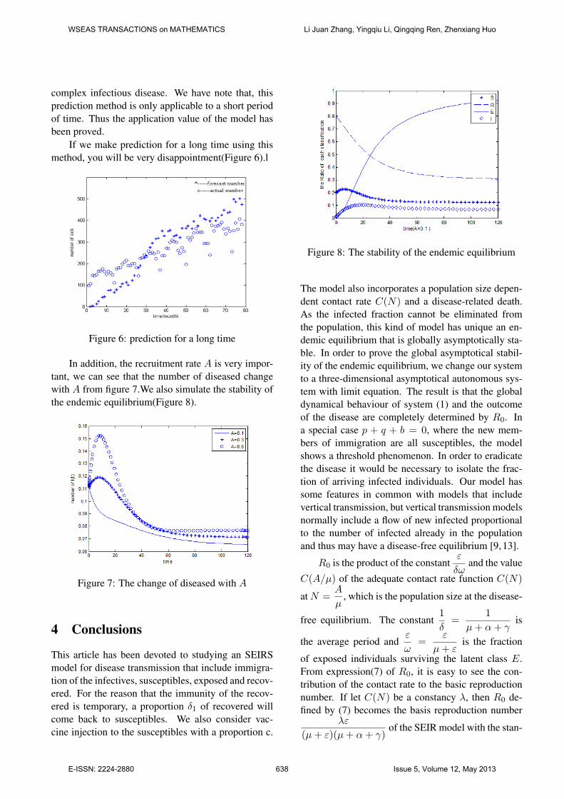
Figure 8: The stability of the endemic equilibrium

The model also incorporates a population size depen-dent contact rate C(N) and a disease-related death.As the infected fraction cannot be eliminated fromthe population, this kind of model has unique an en-demic equilibrium that is globally asymptotically sta-ble. In order to prove the global asymptotical stabil-ity of the endemic equilibrium, we change our systemto a three-dimensional asymptotical autonomous sys-tem with limit equation. The result is that the globaldynamical behaviour of system (1) and the outcomeof the disease are completely determined by R0. Ina special case p + q + b = 0, where the new mem-bers of immigration are all susceptibles, the modelshows a threshold phenomenon. In order to eradicatethe disease it would be necessary to isolate the frac-tion of arriving infected individuals. Our model hassome features in common with models that includevertical transmission, but vertical transmission modelsnormally include a flow of new infected proportionalto the number of infected already in the populationand thus may have a disease-free equilibrium [9, 13].

R0 is the product of the constantε

δωand the value

C(A/µ) of the adequate contact rate function C(N)

atN =A

µ, which is the population size at the disease-

free equilibrium. The constant1

δ=

1

µ+ α+ γis

the average period andε

ω=

ε

µ+ εis the fraction

of exposed individuals surviving the latent class E.From expression(7) of R0, it is easy to see the con-tribution of the contact rate to the basic reproductionnumber. If let C(N) be a constancy λ, then R0 de-fined by (7) becomes the basis reproduction number

λε

(µ+ ε)(µ+ α+ γ)of the SEIR model with the stan-



dard incidenceλSI

Nin [8]. If δ=0, c = 0, the outcome

will be the same to article [10].Finally, we discussed syphilis incidence and

transmission characteristics and predict the develop-ment in China. Computer simulation shows that themodel can reflect the dynamic and immigration be-havioural for disease transmission. So we can takereasonable prevention and intervention methods toprovide reference, basing on the theory.

Acknowledgements: The research was supportedby the Scientific Research Plan Projects for HigherSchools in Hebei Province (Z2012139) and waspartially supported by the Teachers Scientific &Research Fund of China Earthquake Administra-tion(20110116).

References:

[1] H. R. Thieme, Castillo-Chavez C, On the role ofvariable infectivity in the dynamics of the humanimmui-deficiency virus epidemic. In: Castillo-Chavez C, Ed. Mathematical and Statistical Ap-proaches to AIDS Epidemiology (Lect NotesBiomath Vol.83), Berlin, Heidelberg, New York:Springer, 1989, pp.157-177.

[2] R. M. Anderson, Transmission dynamics andcontrol of infectious diseases. In: Anderson RM, May M R, Ed. Population Biology of Infec-tious Diseases, Life Sciences Research Report25, Dahlem Conference. Berlin: Springer, 1982,pp.149-176.

[3] K. Dietz, Overall population patterns in thetransmission cycle of infectious disease agents.In: R. M. Anderson, R. M. May, Ed. PopulationBiology of Infectious Diseases, Berlin, Heidel-berg, New York: Springer, 1982.

[4] D. Greenhalgh, Some results for a SEIR epi-demic model with density dependence in thedeath rate, IMA J.Math Apple Medicine & Bi-ology, No.9, 1992, pp.67-106.

[5] K. Cooke, van den Driessche, Analysis of anSEIRS epidemic model with two delays, J.Math. Biol., 1996, pp.240-260.

[6] D. Greenhalgh, Hopf bifurcation in epidemicmodels with a latent period and nonperma-nent immunity, Math Comput Modelling, Vol.25,No.2, 1997, pp.85-107.

[7] M. Y. Li, J. S. Muldowney, Global stability forthe SEIR model in epidemiology, J. Math Biosci,No.125, 1995, pp. 155-164.

[8] M. Y. Li, R. J. Graef, L. Wang, Global dynamicsof a SEIR model with varying total populationsize, J. Math. Biosci., No.160, 1999, pp.191-213.

[9] Li M Y, Smith H L, Wang L. Global dynamics ofan SEIR epidemic model with vertical transmis-sion, SIAM J Appl Math., Vol.62, No.1, 2001,pp.58-69.

[10] Zhang Juan, Li jianquan, Global Dynamics of anSEIR epidemic Model With Immigration of Dif-ferent Compartments, Acta Mathematica Scien-tia, Vol.26B, No.3, 2006, pp.551-567.

[11] S. Busenberg, K. L. Cooke, Vertical TransmittedDiseases: Models and Dynamics, Biomathemat-ics, Vol 53. Berlin: Springer, 1993.

[12] F. Brauer, Models for Diseases with VerticalTransmission and Nonlinear Population Dynam-ics, J. Math. Biosci., No.128, 1995, pp.13-24.

[13] J. K. Hale, Ordinary Differential Equations,New York: Wiley-Interscience, 1969.

[14] M. Y. Li, J. S. Muldowney, A geometric ap-proach to global stability problems, SIAM JMath Anal., Vol.27, No.4, 1996, pp.1070-1083.

[15] H. R.Thieme, Convergence results and aPoicare-Bendixso trichotomy for asymptoti-cally autonomous differential equations, J. MathBio., No.30, 1992, pp. 755-763.

[16] G. Butler, P. Waltman, Persistence in dynami-cal systems, Proc Amer Math Soc., No.96, 1986,pp.425-430.

[17] Freedman H I, Tang M X, Ruan S G. Uniformpersitence and flows near a closed positively in-variant set, J. Dynam Diff Equat., No.6,1994,pp.583-600.

[18] Smith R A. Some applications of Hausdorffdimension inequalities for ordinary differentialequations. Proc Roy Soc Edinburgh Sect A,No.104, 1986, pp. 235-259.

[19] http://www.moh.gov.cn/publicfiles/business/htmlfiles/mohjbyfkzj/s3578/201207/55376.htm

[20] Jun Li, Linna Wang, Heyi Zheng, SyphilisAerum IgM Antibodies and Infectious [In Chi-nese]. Chinese Journal of Dermatology, Vol.7,No.26, 2012, pp.591-593.



[21] Wanwei Zhou, Yongfang Feng, One Case ofSyphilis in Stage Two [In Chinese], Journalof Clinical Dermatology, Vol.3, No.41, 2012,pp.183-183.

[22] Yi Wang, Jie Xu, Zhijun Li, Mianyang City,Male Sexual Behavior Cohort Baseline of HIV/syphilis infection and analysis of its influencingfactors[In Chinese], Chinese Journal of PublicHealth, Vol.5, No.26, 2012, pp.410-144.



Date post:	17-Apr-2018
Category:	Documents
Upload:	haphuc
View:	229 times
Download:	3 times

Global Dynamics of an SEIRS Epidemic Model with … Dynamics of an SEIRS Epidemic Model with...

Documents