University of Rhode Island University of Rhode Island DigitalCommons@URI DigitalCommons@URI Open Access Dissertations 2019 GLOBAL DYNAMICS OF DISCRETE MONOTONE MAPS IN THE GLOBAL DYNAMICS OF DISCRETE MONOTONE MAPS IN THE PLANE AND IN R PLANE AND IN R N James Marcotte University of Rhode Island, [email protected]Follow this and additional works at: https://digitalcommons.uri.edu/oa_diss Recommended Citation Recommended Citation Marcotte, James, "GLOBAL DYNAMICS OF DISCRETE MONOTONE MAPS IN THE PLANE AND IN R N " (2019). Open Access Dissertations. Paper 1101. https://digitalcommons.uri.edu/oa_diss/1101 This Dissertation is brought to you for free and open access by DigitalCommons@URI. It has been accepted for inclusion in Open Access Dissertations by an authorized administrator of DigitalCommons@URI. For more information, please contact [email protected].
Transcript
University of Rhode Island University of Rhode Island
DigitalCommons@URI DigitalCommons@URI
Open Access Dissertations
2019
GLOBAL DYNAMICS OF DISCRETE MONOTONE MAPS IN THE GLOBAL DYNAMICS OF DISCRETE MONOTONE MAPS IN THE
Follow this and additional works at: https://digitalcommons.uri.edu/oa_diss
Recommended Citation Recommended Citation
Marcotte, James, "GLOBAL DYNAMICS OF DISCRETE MONOTONE MAPS IN THE PLANE AND IN RN" (2019). Open Access Dissertations. Paper 1101. https://digitalcommons.uri.edu/oa_diss/1101
This Dissertation is brought to you for free and open access by DigitalCommons@URI. It has been accepted for inclusion in Open Access Dissertations by an authorized administrator of DigitalCommons@URI. For more information, please contact [email protected].
3. An equilibrium point (x, y) of (3) is locally a saddle point if the charac-
teristic equation has one root that lies inside the unit circle and one root that lies
outside the unit circle, that is, if
|trJT (x, y)| > |1 + detJT (x, y)|
By using these theorems we can characterize each of the equilibrium points of
(3) which gives the local dynamics of (3).
1.3 Monotone Systems of Difference Equations
Since this thesis will be discussing monotone systems of difference equations
throughout, we also provide basic definitions and theorems for monotone systems.
Consider (3) with T the map associated with (3). Then we have the following
definitions and theorems about monotone systems.
Definition 4 The North-east partial order ≤NE is defined by (x, y) ≤NE (w, z)
if and only if x ≤ w and y ≤ z. Also set (x, y) <NE (w, z) if (x, y) ≤NE (w, z)
and (x, y) 6= (w, z), and (x, y) <<NE (w, z) if and only if x < w and y < z. The
South-east partial order ≤SE is defined by (x, y) ≤SE (w, z) if and only if x ≤ w
and y ≥ z. The symbols <SE and <<SE are similarly defined to <NE and <<NE.
Definition 5 A map T is called cooperative if T (x, y) ≤NE T (w, z) whenever
(x, y) ≤NE (w, z). T is called strongly cooperative if T (x, y) <<NE T (w, z) when-
ever (x, y) <NE (w, z). Similarly, a map T is called competitive if T (x, y) ≤SE
5
T (w, z) whenever (x, y) ≤SE (w, z). T is called strongly competitive if T (x, y) <
<SE T (w, z) whenever (x, y) <SE (w, z).
Definition 6 The order interval [p, q]NE is the set [p, q]NE = {x ∈ R2 : p ≤NE
x ≤NE q}. This definition is similar for a South-east order interval.
The following theorem and corollary is a theorem of Dancer and Hess in [2].
Theorem 3 (The Order Trichotomy Theorem) Let X = [a, b], where a < b. Let
the map T : X → X be monotone and T (X) have compact closure in X. Then, at
least one of the following holds:
1. There is a fixed point c such that a < c < b.
2. There exists an entire orbit from a to b that is increasing, and strictly
increasing if T is strictly monotone.
3. There exists an entire orbit from b to a that is decreasing, and strictly
decreasing if T is strictly monotone.
Corollary 1 Let X = [a, b], where a < b and a, b are stable fixed points. Let the
map T : X → X be monotone and T (X) have compact closure in X. Then there
is a third fixed point in [a, b].
These definitions and theorem are essential for understanding the analysis of
monotone systems. The focus of this thesis is to provide some general results for
the basins of attraction of fixed points in some planar cooperative maps.
List of References
[1] E.N. Dancer and P. Hess, Stability of fixed points for order-preserving discretetime dynamical systems, J. reine angew. Math. 419 (1991), 125-129.
[2] Hirsch, M. and Smith, H.L. 2005a. “Monotone dynamical systems”. In Hand-book of Differential Equations, Edited by: Canada, A., Drabek, P. and Fonda,A. Vol. 2, Amsterdam: Elsevier.
6
[3] M. R. S. Kulenovic and O. Merino (2018) Invarient curves for planar competi-tive and cooperative maps, Journal of Difference Equations and Applications,24:6, 898-915, DOI: 10.1018/10236198.2018.1438418
[4] M. R. S. Kulenovic and O. Merino, Discrete Dynamical Systems and DifferenceEquations with Mathematica, Chapman and Hall/CRC, Boca Raton, London,2002.
7
MANUSCRIPT 2
Properties of Basins of Attraction for Planar Discrete CooperativeMaps
M. R. S. Kulenovic1, J. Marcotte and O. Merino
Department of Mathematics,
University of Rhode Island,
Kingston, Rhode Island 02881-0816, USA
Publication status:
Submitted to Discrete and Continuous Dynamical Systems, Ser.B
has three fixed points: the point (0, 0) which is LAS, and the points
10
(−0.617,−0.851) and (0.617, 0.851) which are saddle points. In addition, there
are two repelling minimal period-two points (−1.349, 1.105), (1.349,−1.105). It
can be shown with results from [9] that the basin B of the origin is bounded, and
that ∂B consists of the union of stable manifolds of the two nonzero fixed points,
and that the period two points are endpoints to both manifolds. See figure Figure
2.1 (b). The map G is cooperative and G2 is strongly cooperative.
o
p2
p1
o
p2
p1
q2
q1
(a) (b)
Figure 1. (a) The basin of attraction B of the zero fixed point o of the map T (x, y) =(y, x3 + y3). Note that B is unbounded, and ∂B contains two fixed points p1 and p2
which are saddle points. The union of the stable manifolds of p1 and p2 gives ∂B. (b)The basin of attraction B of the zero fixed point of the map T (x, y) = (y3, x3 + y3). Theset B is bounded, and ∂B contains two fixed points p1 and p2 (saddles) and a repellingminimal period-two pair q1 and q2. The union of the stable manifolds of p1 and p2 gives∂B.
The previous examples suggest the question of whether the geometry of the
basin of locally asymptotically stable fixed or periodic points of planar monotone
maps is particularly simple and amenable to a “nice” characterization.
We note that the maps in (5) and (7) are (locally) invertible, and that in each
of both cases the boundary of the basin B of the origin contains two saddle points.
This allows, by using the results from [9] for example, the characterization of ∂B
as the union of stable manifolds of the saddle points. However, local invertibility
of a cooperative or competitive map is not always true. Also, there is the question
of the components of the basin of attraction in other cases, in addition to the
11
possible presence of other fixed points (perhaps nonhyperbolic) on the boundary
of the basin.
In general, the basin of attraction B(E) of locally asymptotically stable fixed
point E of a map T satisfies
B(E) =∞⋃k=0
T−kB0(E), (8)
where B0(E) is a largest connected invariant set containing E, and T 0 is the identity
function. The problem of characterization of B(E) is finding the properties of
T−kB0(E) for an arbitrary map. In this paper we show that if T is a monotone
(cooperative or competitive) map, one can characterize those components of the
basin of attraction. Our main results will show that the previous two examples are
indicative of the structure of such basin of attraction. In addition, the components
of the basin form an unordered chain of non-invariant sets which eventually map
into B0(E). These components will be ordered in the south-east ordering which
we define next.
This paper is organized as follows. In the rest of this section we give some
basic notions about monotone maps in the plane. The second section presents our
main results and some corollaries. The third section presents examples and the
fourth section gives proofs of the main results.
Consider a partial ordering � on R2. Two points x, y ∈ R2 are said to be
related if x � y or x � y. Also, a strict inequality between points may be defined
as x ≺ y if x � y and y 6= x. A stronger inequality may be defined as x =
(x1, x2) � y = (y1, y2) if x � y with x1 6= y1 and x2 6= y2. If x � y, the order
interval [x, y] is the set {z : x � z � y}. A map T on a nonempty set R ⊂ R2 is a
continuous function T : R → R. A point x in R is a fixed point of T if T (x) = x.
The basin of attraction of a fixed point x of a map T , denoted as B(x), is defined
12
as the set of all initial points x0 for which the sequence of iterates T n(x0) converges
to x. The map T is monotone if x � y implies T (x) � T (y) for all x, y ∈ R, and
it is strongly monotone on R if x ≺ y implies that T (x) � T (y) for all x, y ∈ R.
The map is strictly monotone on R if x ≺ y implies that T (x) ≺ T (y) for all
x, y ∈ R. Throughout this paper we shall use the North-East ordering (NE) for
which the positive cone is the first quadrant, i.e. this partial ordering is defined
by (x1, y1) �ne (x2, y2) if x1 ≤ x2 and y1 ≤ y2 and the South-East (SE) ordering
defined as (x1, y1) �se (x2, y2) if x1 ≤ x2 and y1 ≥ y2. A map T on a nonempty
set R ⊂ R2 which is monotone with respect to the North-East ordering is called
cooperative and a map monotone with respect to the South-East ordering is called
competitive. If T is continuously differentiable on an open set, a sufficient condition
for T to be strongly cooperative (respectively, strongly competitive) is that at every
point of the set, the jacobian matrix has positive entries (resp. positive diagonal
entries and negative off-diagonal entries). For x ∈ R2, define Qi(x) for i = 1, . . . , 4
to be the usual four quadrants based at x and numbered in a counterclockwise
direction, for example, Q1(x) = {y ∈ R2 : x �ne y}. A set A is said to be order
convex if for every x, y ∈ A, the order interval [x, y] is a subset of A. A general
reference for difference equations and maps is [2]. For some basic notions about
monotone discrete systems in the plane, see [1, 5, 6, 7, 8, 9, 10, 18].
2.2 Main Results
The main result applies to cooperative maps on an order interval whose k-th
power (for some k ≥ 1) is strongly cooperative. Smoothness of the map is not
assumed, but it is considered later in Theorems 5 and 6. Unbounded domains
are discussed in Remark 2, competitive maps in Remark 3, and periodic points in
Remark 5.
Theorem 4 Let R be an order interval in R2 with nonempty interior, and let
13
T : int(R) → int(R) be a cooperative map whose k-th power (for some k ≥ 1)
is strongly cooperative. Suppose x ∈ R, and set B := {x ∈ int(R) : Tm(x) →
x as m → ∞}. If there exists an open set O′ in R2 containing x such that
O := O′ ∩ int(R) ⊂ B, then
(i) The boundary of each connected component B′ of B is the union of two curves
C− and C+ (termed the lower and upper boundary curves of B′, respectively).
Points on a boundary curve that are interior to R are non-comparable. The
boundary curves C− and C+ have common endpoints, and these are their only
common points.
(ii) If B′ and B′′ are any two distinct components of B, then either B′ <<se B′′
or B′′ <<se B′.
(iii) Denote with B∗ the connected component of B whose closure in R contains
x. The set B∗ is T -invariant. The intersection of each boundary curve of B∗
with the interior of R is T -invariant.
(iv) If B′ is a component of B such that B′ 6= B∗, then there exists a positive
integer n that depends on B′ such that T n−1(B′) ∩ B∗ = ∅ and T n(B′) ⊂ B∗.
If C ′± and C± are the boundary curves of of B′ and B∗ respectively, set C ′± :=
C ′± ∩ int(R) and C± := C± ∩ int(R). Then T n(C ′−) ⊂ C− and T n(C ′+) ⊂ C+
Remark 1 If in Theorem 4 the point x is in int(R), then x is a fixed point and
the set B is the basin of attraction of x in int(R). However, the map need not be
defined at x for Theorem 4 to apply, see Example 2 in Section 2.3.
Remark 2 The conclusions of Theorem 4 are valid for maps T on unbounded
domains R of either one is of the forms {x : x � p}, {x : p � x}, or R2. To prove
this, consider the natural extension of the partial order to the extended plane
14
R2 = [−∞,∞] × [−∞,∞]. The set R is a subset of R2. Also modify the notion
of boundary curve so that points common to a boundary curve and the boundary
of the domain of the map may have one or both coordinates equal to −∞ or +∞.
The proof is essentially the same as that for Theorem 4. See Example 1 in Section
2.3, where the domain of the map is R2.
R
txC+C−
B∗
B′
B′′
R
C+
C−
pt
vx
B
(a) (b)
Figure 2. (a) the basin B of the fixed point x has three components B′, B∗, B′′ whoseclosure is in int(R) and such that B′ <<se B∗ <<se B′′. Each component has boundarycurves C+ and C−. (b) The set B has only one component, which has part of its boundaryin ∂R. Also, x ∈ ∂R. The point p is an endpoint of both boundary curves C− and C+.The point p is a fixed point of T .
By (i) and (iii) of Theorem 4, the set of endpoints of the boundary curves C+
and C− of B∗ that belong to int(R) is invariant. Such set has at most two points
in int(R), hence any such point is periodic with period two. Therefore we have
the following result.
Corollary 2 Let p be an endpoint of a boundary curve of B∗. If p is in int(R),
then p is a fixed point or a minimal period-two point of T .
From (ii.) of Theorem 4 and Corollary 2 we have the following result.
15
Corollary 3 If there are no period-two points in Q2(x)∪Q4(x) other than x, then
there is only one component of B, and the corresponding boundary curves have
endpoints on R.
Smoothness of the map implies that the boundary of the basin B in Theorem
4 is guaranteed to have additional properties.
Theorem 5 Let R, T and B be as in Theorem 4. Assume the hypotheses of
Theorem 4. Suppose z is a minimal period k point of T in int(R) ∩ ∂B, and that
T is of class C1 in a neighborhood of z. If the jacobian matrix of T k at z has
positive entries, then ∂B is tangential at z to the line ` with direction given by
the eigenspace associated to the characteristic value of T at z with the smallest
modulus.
Theorem 6 Assume the hypotheses of Theorem 4. Suppose T is a continuously
differentiable map on int(R) such that the jacobian matrix at every point in int(R)
has positive entries. Let B′ be a component of the basin B of x, and let C− and C+
be the corresponding boundary curves. Then,
i. Each of the curves C− and C+ of B′ is the graph of a Lipschitz function of a
real variable.
ii. If C− and C+ intersect at a hyperbolic periodic point p ∈ int(R), then p is a
source.
Remark 3 A version of Theorems 4, 5 and 6 and corollaries 2 and 3 are valid
for maps T that are competitive (instead of cooperative). To obtain these results,
replace the word cooperative by the word competitive, and replace the north-east
partial order by the south-east partial order and vice-versa. With these modifica-
tions, the proofs carry over word for word, so those will be omitted. See Example
2 in Section 2.3.
16
Remark 4 If the boundary of the set B∗ in Theorem 4 has a fixed or periodic
saddle point, the local stable manifold can be extended to a global stable manifold
by using topological arguments or results such as those in [9]. In these cases it
is possible to obtain a description of ∂B∗. But often the sufficient conditions for
global stable manifold are difficult to verify or are not applicable at all. In these
cases, Theorems 4, 5, 6 and corollaries give the existence of invariant Lipschitz
curves where other methods fail.
Remark 5 The results of this section are applicable to locally asymptotically
stable minimal period k points p of a map T . To do this, consider the iterates p,
T (p),. . . , T k−1(p) as a fixed points of T k. The basin of the orbit of p is then the
union of the basins of points of the orbit as fixed points of T k.
2.3 Examples
In this section we provide two applications. Example 1 is a discussion on the
global dynamics of a strongly cooperative map whose domain is R2. We show that
the origin is LAS, with basin of attraction that has more than one component.
Admittedly the example is somewhat contrived, but it is the only example of co-
operative map known to the authors with the property that the basin of attraction
of a point consists of several components. A feature of the method used to pro-
duce the example is that it can be used to generate other examples with basins
of attraction consisting of many components, even a countably infinite number of
them. In Example 2 we consider a class of parametrized competitive maps defined
on the nonnegative quadrant minus the origin. The maps have the origin as a
singular point that has a substantial substantial set attracted to it. Our results in
this paper can be applied to characterize the boundary of the set attracted to the
origin. This characterization is valid for all values of the parameters.
17
Example 1 We begin by defining a cooperative map U on the plane for which
the origin is a LAS fixed point with unbounded basin of attraction. Then a map
V is defined as a specific perturbation of U , so that the origin has bounded basin
p4(12.798,−12.798). See Figure 6. The invariant component of the basin of
19
y = ϕ( t )
y = t
0 a b c dt
a
y
Figure 4. Graphs of φ from (13) and the identity function on the nonnegative semi axis.φ has locally asymptotically stable fixed points 0, b = 2.06, and a repelling fixed pointa = 0.95. The real numbers c = 6.03 and d = 12.80 are pre-images of a. The basin ofattraction of 0 on the semi-axis consists of the intervals 0 ≤ t < a and c < t < d. Alldecimal numbers have been rounded to two decimals.
z = V11(x, y) z = V12(x, y) z = V21(x, y) z = V22(x, y)
Figure 5. The partial derivatives of V (x, y). Also shown in the plane z = 0.
attraction of the origin is bounded by the global stable manifolds of two saddle
fixed points which have endpoints at period-two points.
Example 2 Consider maps of the form
T (x, y) :=
(x3
αx+ (1− α) y,
y3
(1− δ)x+ δ y
), (x, y) ∈ R2
+ \ {0, 0}, α, δ ∈ (0, 1)
(14)
The map T is competitive on its domain and strongly competitive on its interior,
the open positive quadrant, as can be concluded from the jacobian matrix
(x2 ( 2xα+3 y (1−α) )
((αx+(1−α) y)2 − x3 (1−α)((αx+(1−α) y)2
− y3 (1−δ)((δ)x+δ y)2
y2 (2 y δ−3x(δ−1))((1−δ)x+δ y)2
)(15)
The origin o is a singular point, and there are three fixed points, namely
a(α, 0), d(0, δ) and b(1, 1). A straightforward calculation gives that a and d are
20
s
p1 p2
p3
p4
r
q1
q2
q3
q4q1
p1
o
r
s
(a) (b)
Figure 6. (a) Three components of the basin of attraction of the fixed point zero ofthe map V (x, y) in Example 1. Here r, s are saddle fixed points, p1 and q1 are a saddleperiod-two pair, p2 and q2 are repelling fixed points, and p3, p4, q3, q4 are eventualperiod-two points. The boundary of the invariant part of the basin of attraction consistof stable manifolds of saddle fixed points with a period-two endpoints. In addition, thereare two eventually period-two points which are end points of another piece of the basinof attraction which is mapped into the invariant part. (b) The invariant component ofthe basin of the origin o.
saddle points, each with an open semiaxis as unstable manifold. Also b is a repeller,
with characteristic values 2, 4 − α − δ, and corresponding eigenvectors (1, 1) and
(α− 1, 1− δ). The ray {(x, x) : x > 0}, is invariant, more specifically we have
T (x, x) = (x2, x2) for all x > 0, α, δ ∈ (0, 1). (16)
The following is a complete characterization of the global dynamics of map
(14) for all allowed values of the parameters. See Figure 7.
Proposition 1 Let T be as in (14). For all values of α and δ in (0, 1), the set
B := {(x, y) : T n(x, y)→ (0, 0)} is bounded by north-east ordered Lipschitz curves
C+ and C−, which have endpoints a, b and d, b respectively. Also, C+ and C− are
tangential to the line y = x at the point b. If (x, y) 6= b is in C+ (resp. C−) then
21
T n(x, y) → a (resp. T n(x, y) → d), while if (x, y) is in the complement of the
closure of B, then ‖T n(x, y)‖ → ∞.
d
ao
b
C+
C−
B
Figure 7. Global dynamics for map (14) as given in Proposition 1. Here α = 0.4 andδ = 0.7.
Proof. We begin by verifying that the origin has a relative neighborhood that is
a subset of B. This can be seen as follows. The relations T (x, 0) �se (x, 0) for
0 < x < α, and (0, y) �se (0, y) for 0 < y < δ imply that for (u, v) with 0 < u < x
and 0 < v < y, T n(0, y) �se T n(u, v) �se T n(x, 0). Since T n(x, 0) → (0, 0) and
T n(0, y) → (0, 0), we have T n(u, v) → (0, 0). Thus the set O′ = {(x, y) : 0 < x <
α , 0 < y < δ} satisfies O′ ⊂ B. Therefore the hypotheses of Theorems 4, 5 and 6
are satisfied.
We now show that B has only one component. By Theorem 4, all components
of B are non-comparable in the south-east ordering, therefore they are comparable
in the north-east ordering. By (16) the open line segment L := {(x, x) : 0 <
x < 1} consists of points (x, x) such that T n(x, x) → (0, 0). Also by (16) the ray
S := {(x, x) : 1 < x <∞} consists of points (x, x) such that ‖T n(x, x)‖ → ∞. For
any point (z, w) with z > 1 or w > 1 one may choose x so that (x, x) �se (z, w) or
22
(z, w) �se (x, x). It follows T n(x, x) �se T n(z, w) or T n(z, w) �se T n(x, x). Since
T n(x, x) = (x2n, x2
n), we have ‖T n(z, w)‖ → ∞. In particular, it follows that B
has only one component.
Note {a, d, b } ⊂ ∂B. Let C− and C+ be as in Theorem 4. Since no points
outside of the unit square belong to B, it follows that b is an endpoint of both
C+ and C−. Also a is an endpoint of C− and d is an endpoint of C+, due to the
fact that the axes are unstable manifolds of a and d. The rest of the proposition
follows from Theorems 4, 5 and 6, and their corollaries. 2
2.4 Proofs
Proof of Theorem 4. It is sufficient to consider the case where T is strongly
monotonic. To see this, let T , B, k and O be as in Theorem 4, and let Bk :=
{x ∈ int(R) : Tmk(x) → x as m → ∞}. If x ∈ Bk, then Tmk(x) ∈ O for m
large enough, which implies x ∈ B. Thus Bk ⊂ B, and since B ⊂ Bk it follows
B = Bk. Without loss of generality we assume for the rest of this section that T is
a strongly monotonic map (k = 1).
We prove several claims first. The first two claims are about certain properties
of B and its boundary set.
Claim 1 The set B is open and order convex, and it has either a finite or countably
infinite number of connected components.
Proof. If x ∈ B, then for sufficiently large m ∈ N we have Tm(x) ∈ O. Then
x is an element of (Tm)−1(O), which is an open subset of B. Thus B is open.
If {x, z} ⊂ B, then by monotonicity of T , for every y ∈ int(R) and all m ∈ N,
x � y � z implies Tm(x) � Tm(y) � Tm(z). Hence Tm(y)→ x and we conclude B
is order-convex. If the number of connected components of B is not finite, choose
a point in each of the components with rational entries. The collection of such
points is countable, hence so is the collection of components of B. 2
23
Claim 2 The set ∂B does not contain a linearly ordered line segment contained
in int(R).
Proof. Arguing by contradiction, suppose ∂B contains a �ne linearly ordered line
segment L(x, z) ⊂ int(R). Choose y a point In L(x, z) with y 6= x, z. Then T (x) <
<ne T (y) <<ne T (z) by strong monotonicity of T . But then V <<ne T (y) <<ne W
for some open neighborhoods V of T (x) and W of T (z). Now both V and W
contain points in B, say v and w. In particular, v <<ne T (y) <<ne w. Since B is
order-convex, it follows that T (y) ∈ B, which contradicts invariance of ∂B. 2
We now proceed to define functions φ± of a real variable that are key to
establishing further properties of the boundary of B. Denote with π1 the projection
operator on R2 given by π1(x, y) = x. Let I := π1(B), that is, I is the set consisting
of all t in R for which there exists y in R such that (t, y) ∈ B. The set I is open
in R, and it has a finite or countable number of connected components (intervals).
For each connected component of I choose a rational number q in the component,
and label the component as Iq. Let Q be the set consisting of all such indices
q. Then for each q ∈ Q, the sets Iq are open in R, pairwise disjoint, and satisfy
Rearranging terms in (29) and using (28) and (30) we have
T (tn, φ(tn))− T (t∗, φ(t∗))
= (tn − t∗)(a+ g
(1)n + (b− g(1)n )φ(tn)−φ(t∗)
tn−t∗ , c+ g(2)n + (d− g(2)n )φ(tn)−φ(t∗)
tn−t∗
).
(31)
By (28) and (30) and the assumption that a, b, c and d are positive, both co-
ordinates in the right-hand side of (31) are negative for large n, and therefore
T (tn, φ(tn)) � T (t∗, φ(t∗)). But this contradicts (i) of Theorem 4, which requires
points on C+ to be non-comparable. Thus φ is Lipschitz.
(ii) We present the proof for the case when p is a fixed point of T . Note p is
necessarily unstable since p ∈ ∂B. Since it is hyperbolic, it is either a saddle point
or a source. If p is a saddle point, then it has a local stable manifold M s, which is
tangential to v with v not comparable to the origin by the Krein-Rutman theorem.
There exist points x in B∗ that are arbitrarily close to p and which belong to to the
union of quadrants Q2(p) and Q4(p). Furthermore, such points x may be chosen
to be comparable to points on M s, which would prevent the iterates of such points
from converging to p, thus contradicting the definition of stable manifold. 2
31
List of References
[1] A. Brett and M. R. S. Kulenovic, Basins of Attraction of Equilibrium Pointsof Monotone Difference Equations. Sarajevo J. Math., 5(18): 211–233, 2009.
[2] S. Elaydi, An introduction to difference equations. Third edition. Undergrad-uate Texts in Mathematics. Springer, New York, 2005.
[3] M. Garic-Demirovic, M. R. S. Kulenovic and M. Nurkanovic, Basins of At-traction of Certain Homogeneous Second Order Quadratic Fractional Differ-ence Equation, Journal of Concrete and Applicable Mathematics, Vol. 13 (1-2)(2015), 35-50.
[4] J. Guckenheimer and P. Holmes, Nonlinear oscillations, dynamical systems,and bifurcations of vector fields. Revised and corrected reprint of the 1983original. Applied Mathematical Sciences, 42. Springer-Verlag, New York, 1990.
[5] P. Hess, Periodic-parabolic boundary value problems and positivity, PitmanResearch Notes in Mathematics Series, 247. Longman Scientific and Technical,Harlow; copublished in the United States with John Wiley and Sons, Inc., NewYork, 1991.
[6] M. Hirsch and H. Smith, Monotone Dynamical Systems, Handbook of Differ-ential Equations, Ordinary Differential Equations (second volume), 239-357,Elsevier B. V., Amsterdam, 2005.
[7] M. Hirsch and H. L. Smith, Monotone Maps: A Review, J. Difference Equ.Appl. 11(2005), 379-398.
[8] M. R. S. Kulenovic and O. Merino, Global Bifurcations for Competitive Sys-tems in the Plane, Discrete Contin. Dyn. Syst. Ser. B 12(2009), 133–149.
[9] M. R. S. Kulenovic and O. Merino, Invariant manifolds for planar competitiveand cooperative maps, Journal of Difference Equations and Applications, Vol.24 (6) (2018), 898-915.
[10] M.R.S. Kulenovic, O. Merino and M. Nurkanovic, Global dynamics of cer-tain competitive system in the plane, Journal of Difference Equations andApplications, Vol. 18 (12) (2012), 1951-1966.
[11] M.R.S. Kulenovic, S. Moranjkic and Z. Nurkanovic Global Dynamics and Bi-furcation of a Perturbed Sigmoid Beverton-Holt Difference Equation, Mathe-matical Methods in Applied Sciences, 39(2016), 2696–2715.
[12] S. W. McDonald, C. Grebogi, E. Ott and J. A. Yorke, Fractal basin bound-aries. Phys. D 17 (1985), no. 2, 125–153.
[13] J. W. Milnor (2006) Attractor. Scholarpedia, 1(11):1815
32
[14] H. E. Nusse and J. A. Yorke, Basins of attraction. Science 271 (1996), no.5254, 1376–1380.
[15] H. E. Nusse and J. A. Yorke, The structure of basins of attraction and theirtrapping regions. Ergodic Theory Dynam. Systems 17 (1997), no. 2, 463–481.
[16] H. E. Nusse and J. A. Yorke, Characterizing the basins with the most entan-gled boundaries. Ergodic Theory Dynam. Systems 23 (2003), no. 3, 895–906.
[17] H. E. Nusse and J. A. Yorke, Bifurcations of basins of attraction from theview point of prime ends. Topology Appl. 154 (2007), no. 13, 2567–2579.
[18] H.L. Smith, Planar competitive and cooperative difference equations, Journalof Difference Equations and Applications, Vol. 3, No.5-6,335-357,1998.
33
MANUSCRIPT 3
Global Dynamics Results for Discrete Planar Cooperative Maps
M. R. S. Kulenovic1, J. Marcotte and O. Merino
Department of Mathematics,
University of Rhode Island,
Kingston, Rhode Island 02881-0816, USA
Publication status:
Submitted to Journal of Difference Equations and Appl.
where the transition functions f, g are non-decreasing in all its arguments and its
corresponding map F = (f, g). Sufficient conditions are given for such planar
cooperative map to have the qualitative global dynamics determined by local sta-
bility information obtained from fixed and minimal period-two points. The results
are given for a class of strongly cooperative planar maps of class C1 defined on an
order interval. The maps are assumed to have a finite number of strongly ordered
fixed points and minimal period-two points. Our results holds in hyperbolic case as
well as in some non-hyperbolic cases as well. Our results are motivated by global
dynamic results for the systems
xn+1 = a xn +b ynδ + yn
yn+1 =c xnδ + xn
+ d yn, n = 0, 1, . . .(33)
35
and
xn+1 = a xn +b y2nδ + y2n
yn+1 =c x2nδ + x2n
+ d yn, n = 0, 1, . . . .(34)
see [3, 4, 5, 17]. System (33) was considered in [3] and it was proved that all
bounded solutions exhibited global attractivity to either the zero equilibrium or
to the unique positive equilibrium. More precisely, it was shown in [3] the global
dynamics of system (33) where a, b, c, d, δ > 0, x0, y0 ≥ 0 is simple and can be de-
scribed in terms of bifurcation theory as the transcritical bifurcation which causes
an exchange of stability when (1− a)(1− d)δ2 − bc passes through the value 0.
The system (34), studied in [4] exhibited the appearance of period-two solu-
tions, which played an important role in the global dynamics of this system. Cases
where provided for such system which had 1, 2 or 3 period-two solutions and in
the last case one of these period-two solutions had substantial basin of attraction
[4]. Papers [3, 4] extensively used the algebraic techniques to find the regions of
existence and stability of equilibrium solutions and period-two solutions. The re-
sults in this paper will be proven through the geometric analysis of the equilibrium
curves and by using some major results about the global stable and unstable man-
ifolds of cooperative systems in the plane [21]-[24]. The results of this paper are
applicable to systems (33) and (34). Our results have immediate extension to the
competitive systems of difference equations in the plane.
The paper is organized as follows. In Section 3.2 we list some basic results
that are relevant to this paper, see [21]-[24]. See also [1, 2, 6, 9, 10, 11, 12, 15,
16, 19, 20, 25, 26, 27, 28] for some related competitive systems. In Section 3.3
we present the three main theorems. In section 3.4 we apply the theorems from
Section 3.3 to a parametrized cooperative system whose transition functions are of
the Holling’s type [17]. Finally the proofs of the results in Section 3.3 are presented
36
in Section 3.5.
3.2 Preliminaries
Let � be a partial order on Rn with nonnegative cone P . For x, y ∈ Rn the
order interval Jx, yK is the set of all z such that x � z � y. We say x ≺ y if x � y
and x 6= y, and x � y if y − x ∈ int(P ). A map T on a subset of Rn is order
preserving if T (x) � T (y) whenever x ≺ y, strictly order preserving if T (x) ≺ T (y)
whenever x ≺ y, and strongly order preserving if T (x)� T (y) whenever x ≺ y.
Let T : R→ R be a map with a fixed point x and let R′ be an invariant subset
of R that contains x. We say that x is stable (asymptotically stable) relative to
R′ if x is a stable (asymptotically stable) fixed point of the restriction of T to
R′. The basin of attraction of a fixed point x, denoted as B(x) is defined as
B(x) = {y : T n(y) → x}. Subsolution (resp. supersolution) for the map T is a
point which satisfies x � T (x) (resp. T (x) � x). A fixed point u ∈ V is said to be
order stable from below if there exists a strictly increasing sequence of subsolutions
vn in V convergent to u. A fixed point u ∈ V is said to be strongly order stable
from below if there exists a strictly increasing sequence of strict subsolutions vn
in V convergent to u. The notions of order stable from above and strongly order
stable from above are defined similarly. A (strongly) order stable fixed point has
the respective stability property from above and below [7].
Throughout this paper we shall use the North-East ordering (NE) for which
the positive cone is the first quadrant, i.e. this partial ordering is defined by
(x1, y1) �ne (x2, y2) if x1 ≤ x2 and y1 ≤ y2 and the South-East (SE) ordering
defined as (x1, y1) �se (x2, y2) if x1 ≤ x2 and y1 ≥ y2.
A map T on a nonempty set R ⊂ R2 which is monotone with respect to the
North-East (NE) ordering is called cooperative and a map monotone with respect
to the South-East (SE) ordering is called competitive. A map T on a nonempty
37
set R ⊂ R2 which second iterate T 2 is monotone with respect to the North-East
(resp. South-East) ordering is called anti-cooperative (resp. anti-competitive).
If T is differentiable map on a nonempty set R, a sufficient condition for T to
be strongly monotone with respect to the NE ordering is that the Jacobian matrix
at all points x has the sign configuration
sign (JT (x)) =
[+ +
+ +
], (35)
provided that R is open and convex.
The next result in [24] is stated for order-preserving maps on Rn. See [14] for
a more general version valid in ordered Banach spaces.
Theorem 7 For a nonempty set R ⊂ Rn and � a partial order on Rn, let T : R→
R be an order preserving map, and let a, b ∈ R be such that a ≺ b and Ja, bK ⊂ R.
If a � T (a) and T (b) � b, then Ja, bK is an invariant set and
i.) There exists a fixed point of T in Ja, bK.
ii.) If T is strongly order preserving, then there exists a fixed point in Ja, bK which
is stable relative to Ja, bK.
iii.) If there is only one fixed point in Ja, bK, then it is a global attractor in Ja, bK
and therefore asymptotically stable relative to Ja, bK.
The following result is a direct consequence of the Trichotomy Theorem, see
[14, 24], and is helpful for determining the basins of attraction of the equilibrium
points.
Corollary 4 If the nonnegative cone of a partial ordering � is a generalized quad-
rant in Rn, and if T has no fixed points in Ju1, u2K other than u1 and u2, then the
38
interior of Ju1, u2K is either a subset of the basin of attraction of u1 or a subset of
the basin of attraction of u2.
Next result is a simple and useful geometric test for checking when the fixed
point of the cooperative map is non-hyperbolic.
Lemma 2 Let (x, y) be an interior fixed point of a cooperative map R(x, y) =
(f(x, y), g(x, y)), and let r be the spectral radius of the Jacobian matrix JR(x, y).
Suppose the tangent lines to f(x, y) = x and g(x, y) = y at (x, y) are not parallel
to one of the axes. Denote with m1 and m2 respectively the slopes of the tangent
lines. The following statements are true:
(i) If 0 < m2 < m1, then r < 1.
(ii) If 0 < m1 = m2, then r = 1.
(iii) If 0 < m1 < m2, then r > 1.
Proof. Without loss of generality assume (x, y) = (0, 0). Let J =(α βγ δ
)be the
jacobian of R at the origin. Note the tangent lines to f(x, y) = x and g(x, y) = y
at (0, 0) are given by αx + β y = x and γ x + δ y = y. Thus the entries of J are
nonzero, and m1 and m2 are respectively the slopes of the lines αx+ β y = x and
γ x + δ y = y. Since m1 = (1 − α)/β and m2 = γ/(1 − δ), from m1 > 0 and
m2 > 0, we obtain 0 < α < 1 and 0 < δ < 1. The characteristic polynomial of J ,
p(t) := t2 − (a + d) t + a d − b c, has real and distinct roots s and r, with |s| < r.
Then,
m1 −m2 =1− αβ− γ
1− δ=
1− α− δ + α δ − β γβ(1− δ)
=p(1)
β(1− δ)(36)
Note the minimum of y = p(t) is attained at t = α+δ2
< 1. If m1 > m2, then
p(1) > 0, which implies r < 1. If m1 = m2, then p(1) = 0, hence r = 1. Similarly,
if m1 < m2, then p(1) < 0, so r > 1 in this case. 2
39
3.3 Main Results
In this section we present three theorems. Theorem 8 gives a qualitative
characterization of global dynamics of a class of bounded planar cooperative maps.
The maps are assumed to have hyperbolic fixed points that are strongly ordered
and to have no minimal period-two points. A result for maps with a non-hyperbolic
fixed point is considered in Theorem 9. If minimal period-two points are present,
Theorem 10 gives information that in many situations is sufficient to produce a
description of the global dynamics of the map.
Suppose R = [a, b] is an order interval in R2, and T : R → R is a given
cooperative map. When the number of fixed points of T is one or two, global
dynamics of T can be determined from basic properties of monotone maps and the
The Trichotomy Theorem [15]. Indeed, since T is continuous andR is compact and
connected, T must have a fixed point. If the fixed point is unique, by monotonicity
of T it is a global attractor. Now suppose T has exactly two fixed points x and y
such that x ≺ y. Then a is a supersolution and b is a subsolution, and therefore
∩∞n=0Tn([a, b]) = [x, y]. The Trichotomy Theorem implies that one fixed point
is order stable and the other one is unstable, with the interior of [x, y] being
attracted to either x or y. For bounded strongly cooperative maps with three or
more hyperbolic strongly ordered fixed points and with no minimal period-two
points, the following result gives a qualitative global dynamics description.
Theorem 8 Let R be an order interval (with respect to the north-east ordering)
in R2. Let T : R → R be a map that is strongly cooperative, bounded, and of
class C1 in the interior of R. Assume (H1) The set F of fixed points of T satisfies
3 ≤ |F| < ∞, (H2) F is strongly ordered, and (H3) F ∩ int(R) consists only of
hyperbolic fixed points.
If T has no minimal period-two points, then there exists an integer k with
40
1 ≤ k ≤ |F| − 2, and there exist k invariant strongly south-east ordered pairwise
disjoint curves C1, . . . , Ck in R such that C` has endpoints in ∂R, C` contains a
fixed point of T and only one. Every orbit in C` converges to the fixed point in C`,
which is a saddle fixed point. Each connected component of R \ ∪{C1, . . . , Ck} is
the basin of attraction of an order stable fixed point.
Corollary 5 If T has no interior repelling fixed points, then every orbit converges
to a fixed point.
The following result is useful in the study of planar cooperative maps with non-
hyperbolic fixed points.
Theorem 9 For a, b ∈ R2 with a ≺ b, let T : [a, b]→ [a, b] be a strongly coopera-
tive map that is of class C1 in the interior of [a, b] and such that
(H1) a and b are fixed points of T , and [a, b] contains a unique interior fixed point
c.
(H2) a and c are order stable from above or b and c are order stable from below.
(H3) There are no minimal period-two points in [a, b].
Then there exists a strongly south-east ordered invariant Lipschitz curve C through
c and with endpoints on the boundary of [a, b], such that each of the two connected
components of [a, b] \ C is a subset of the basin of attraction of a fixed point. Also,
for x ∈ C, T n(x)→ c.
Remark 6 By hypothesis (H1) of Theorem 9, in (H3) it is enough to require
x ∈ Q2(c) ∩ Q4(c). Also, hypothesis (H2) implies that the spectral radius of the
jacobian matrix of T at c equals 1. In particular, c is non-hyperbolic.
41
If a bounded strongly cooperative map T with T : R → R has a minimal
period-two point p, then there exist fixed points a and b such that p is in the
interior of [a, b]. Indeed, just choose x and y in R such that x � z � y for all
y ∈ T (R). Then x � T (x) and T (y) � y, that is, x is a super solution and y
is a sub solution. Both have bounded iterates that satisfy T n(x) ≺ p ≺ T n(y),
for n = 1, 2, . . .. Such iterates must converge to fixed points a and b such that
a ≺ p ≺ b. The next result implies that, under hypotheses that include (among
others) the non-existence of minimal period-four points and the existence of a
unique interior fixed point, the global dynamics picture of T on [a, b] is quite
simple.
Theorem 10 For a, b ∈ R2 with a ≺ b, let T : [a, b] → [a, b] be a strongly
cooperative map that is of class C1 in the interior of [a, b] and such that
(H1) a and b are order stable fixed points of T , and [a, b] contains a unique interior
fixed point c,
(H2) There are no minimal period-four points in [a, b].
(H3) If x ∈ [a, b] satisfies T (x) = c, then x = c.
(H4) The smaller characteristic value of T at each fixed point or minimal period-
two point in [a, b] is not −1.
Then the following statements are true.
(i) If {p1, T (p1)} is a unique minimal period two orbit in [a, b], then c is a
repeller and p1 is a periodic saddle point. The basins of a and b in [a, b]
have a common boundary in the interior of [a, b] which is a strongly south-
east ordered invariant curve C1 that contains {p1, T (p1)} and c, and that has
endpoints in the boundary of [a, b]. If x ∈ C1 satisfies x 6= c, then T n(x) is
attracted to {p1, T (p1)}.
42
(ii) If {p1, T (p1)} and {p2, T (p2)} are the only minimal period two orbits in [a, b]
and if p1 ≺ p2, then the boundary of the basin of a in the interior of [a, b]
is a strongly south east ordered invariant curve C1 that contains {p1, T (p1)}
and c, and the boundary of the basin of b in the interior of [a, b] is a strongly
south east ordered invariant curve C2 that contains {p2, T (p2)} and c, both
C1 and C2 have endpoints on the boundary of [a, b], and C1 ∩ C2 = {c}. The
point c is a repelling fixed point, one of p1, p2 minimal period-two periodic
point is a saddle, and the other is a non-hyperbolic semistable periodic point.
If x ∈ C1 satisfies x 6= c, then T n(x) is attracted to {p1, T (p1)}. If x ∈ C2
satisfies x 6= c, then T n(x) is attracted to {p2, T (p2)}. The region bounded
R1 bounded by C1 and C2 is invariant. If x ∈ R1, then T n(x) is attracted to
the orbit of the non-hyperbolic periodic point.
(iii) Suppose T has exactly k ≥ 3 minimal period-two orbits
{p1, T (p1)}, . . . , {pk, T (pk)} where p1, . . . , pk are hyperbolic and
p1 ≺ p2 ≺ . . . ≺ pk. Then c is a repelling fixed point, k is odd, and
for 1 ≤ ` ≤ k, p` is a periodic saddle if ` is odd, while p` is LAS if ` is even.
There exist strongly south east ordered invariant curves C1, . . . , C 12(k+1) with
endpoints on the boundary of [a, b] such that for i, j ∈ {1, . . . 12(k + 1)} with
i 6= j, Ci ∩ Cj = {c}, {p2i−1, T (p2i−1)} ⊂ Ci, and {p2i, T (p2i)} is a subset of
the open region Ri bounded by C2i−1 and C2i+1. For every x ∈ Ci that satisfies
x 6= c, T n(x) is attracted to {p2i−1, T (p2i−1)}. For every x in Ri, Tn(x) is
attracted to {p2i, T (p2i)}. The region Ri is invariant. The boundary of the
basin of a (respectively, b) in the interior of [a, b] is C1 (resp. Ck).
Remark 7 Suppose in Theorem 10 the map T has a bounded and smooth strongly
cooperative extension T on a domain R which contains [a, b] so that a and b
are locally asymptotically stable, and such that fixed points are strongly ordered
43
and all minimal period-two points are contained in [a, b]. Assume also T has no
minimal period-four points in R, and that the equation T (x) = c has x = c as its
only solution in R. By Theorem 4 in [18] there exist south-east strongly ordered
curves C+(a) through a and C−(b) through b that are part of the boundary of
the basin of a and b respectively, and so that c ∈ C+(a) ∩ C−(b). Thus necessarily
C ⊂ C+(a)∩C−(b). Now endpoints of both C+(a) and C−(b) belong to the boundary
of R, since otherwise any such endpoint is a fixed point or minimal period-two
point, by Corollary 2 in [18]. This is not possible because of the assumptions
on T . Boundedness of T can now be used to prove that points on both C+(a)
and C−(b) have iterates that converge to a minimal period-two point. Finally, we
prove C+(a) = C−(b). If C+(a) and C−(b) are not the same curve, then points x
and y can be chosen in C+(a) and C−(b) respectively so that x ≺ y. Then for all
n ≥ 1, T n(x) ≺ T n(y). But for n large enough, T n(x) and T n(y) both belong to
C, which is strongly ordered in the southeast order. This contradiction completes
the argument.
3.4 Global dynamics of a cooperative system
The purpose of this section is to illustrate the application of the results in
this paper. Consider the following parametrized system of difference equations of
Holling type:
xn+1 =a xn
δ1 + xn+
b y2nδ2 + y2n
yn+1 =c x2n
δ2 + x2n+
d ynδ1 + yn
, n = 0, 1, 2, . . . (37)
44
where a, b, c, d, δ1, δ2 > 0, x0, y0 ≥ 0. Let T : R2+ → R2
+ be the map associated to
(37), that is
T (x, y) =
(a x
δ1 + x+
b y2
δ2 + y2,c x2
δ2 + x2+
d y
δ1 + y
). (38)
The results in Section 3.3 imply that if certain properties of the map in question are
satisfied, then the qualitative global dynamics pictures of T can be deduced from
the study of fixed and periodic points. We now proceed to establish properties of
the parametrized family of maps.
Proposition 2 For a, b, c, d, δ1, δ2 > 0, let e0 := (0, 0) and u := ( aδ1
+ bδ2, cδ2
+ dδ1
).
Then the map T in (38) is bounded and satisfies T (R2+) ⊂ [e0, u], T is strongly
monotonic on its domain and it is smooth on a neighborhood of R2+. The set F of
fixed points of T is strongly ordered, finite, and contains the origin.
Proof. The jacobian matrix of T at (x, y) is
JT (x, y) =
(a δ1
(x+δ1)22 b δ2
(y2+δ2)22 c x δ2
(x2+δ2)2d δ1
(y+δ1)2
)(39)
Since JT (x, y) has positive entries, T is strongly monotonic on R2+. The increasing
character of the coordinate entries of T with respect to each variable gives that T
is bounded with range [0, aδ1
+ bδ2
)× [0, cδ2
+ dδ1
). By direct substitution in (38) we
have the origin e0 is a fixed point for all values of the parameters. Fixed points of
T are common points of the equilibrium curves
(C1) : x =a x
δ1 + x+
b y2
δ2 + y2(40)
(C2) : y =c x2
δ2 + x2+
d y
δ1 + y(41)
45
It is obvious that the origin is a fixed point. Since (40) and (41) may be written as
polynomial (quartic) equations, Bezout’s theorem gives that there are at most 16
fixed points. For (x, y) in the positive quadrant, (40) and (41) may be rewritten
as
y =
√−δ2 x (x+ δ1 − a)
x2 + (δ1 − a− b)x− b δ1, max(a− δ1, 0) < x < A , (42)
x =
√−δ2 y (y + δ1 − d)
y2 + (δ1 − c− d) y − c δ1, max(d− δ1, 0) < x < B , (43)
where A := 12
(a+ b− δ1 +
√(a+ b− δ1)2 + 4 b δ1
)and B :=
12
(c+ d− δ1 +
√(c+ d− δ1)2 + 4 c δ1
). Some basic calculations that we
skip show that (42) defines y as an increasing function of x in [0, A), and (43)
defines x as an increasing function of y in [0, B). Thus the set F of fixed points
of T is linearly ordered in the north-east order, and F ⊂ [0, A)× [0, B). 2
Proposition 2 establishes that the parametrized family of maps (38) satisfies
some of the hypotheses of the results in Section 3.3. The remaining hypotheses
concern fixed and periodic points. In the present case, number and type of fixed
and periodic points naturally depends on the choice of parameters that appear
in the definition of the map. Equations (40) and (41) are to be solved to obtain
fixed points, but these equations do not lend themselves to a simple criterion
for classifying fixed points; the number of parameters is just too high and the
polynomial equations that can be obtained have a high degree.
Numerical searches performed by the authors of this article suggest that four
is the maximum number of fixed points for system (37), and that three is the
maximum number of minimal period-two orbits.
In the rest of this section we illustrate the application of the results of this
paper for different parameter choices given in Table 1. The different cases are
46
presented in Figures 9 – 14. For specific values of the map T , fixed points and
minimal period-two points can be easily found with a computer algebra system
(CAS). Also a CAS can be used to determine that a specific fixed point has only
one pre-image. CAS do not work to investigate existence of minimal period-four
points algebraically due to the complexity of the equations involved. In this case
one can use other means such as the approach mentioned in Figure 15.
Case a b δ1 c d δ2(1) 0.345 2 1.585 1.04 0.435 0.73(2) 0.500 2 1.585 0.65 0.435 0.73(3) 0.375 2. 0.98 0.505 1.098 0.73(4) 0.347447 5.26514 4.54021 0.774986 0.137048 9.06053(5) 0.277479 8.91088 0.115188 3.74014 0.4013 7.43602(6) 0.277479 8.91088 3.39209 0.331034 0.115188 7.43602
Table 1. Parameter values used in Figs. 9 – 14
47
0 1 20
1
2
e0
e1
C1
C2
0 1 20
1
2
e0
e1
C
(a) (b)
Figure 9. Case 1 in Table 1. There exists a unique interior fixed point e1, which isnon-hyperbolic and stable from above. The origin e0 is stable from above. There are nominimal period-two points. (a) shows the equilibrium curves, which have a tangentialcontact point at e1, as implied by Lemma 2. (b) By Theorem 9 applied to the restrictionof the map to the invariant order interval [e0,u], there exists a southeast ordered curveC through e1, such that points below C are attracted to e0 and points on or above C areattracted to e1. Since there are no period-two points outside [e0, u], the curve C has anextension to a southeast ordered curve on R2
+ with endpoints on the boundary whichseparates the basins of attraction of e0 and e1.
3.5 Proofs of Theorems
Proof of Theorem 8. Denote with x`, ` = 1, . . . ,m the fixed points of T ordered
so that x` ≺ x`+1, for 1 ≤ ` ≤ m − 1. Choose ` ∈ {1, . . . ,m − 1}. Then [x`, x`+1]
has only two fixed points, so by the Trichotomy Theorem one of the fixed points
is stable and the other is unstable. Thus either all even indexed fixed points are
stable, or all odd indexed fixed points are stable. By boundedness of T , interior
unstable fixed points belong to an order interval in R determined by two stable
fixed points. Suppose x` and x`+2 are stable, and x`+1 is unstable. By Theorem 4
and Theorem 6 in [18] there exist south-east ordered Lipschitz curves C`+, C`−, such
that ∂B(x`) = C`+ ∪ C`−, and whose only possible common points are endpoints,
and in this case such points are either fixed points or minimal period-two points.
Neither of those two possibilities is allowed by the hypotheses of the Theorem,
hence endpoints do not coincide. Note that x`+1 ∈ C`+. Thus the dynamics of T
48
0 1 20
1
2
e0
e1
e2
C1
C2
e0
e1
e2
C
(a) (b)
Figure 10. Case 2 in Table 1. There exist interior fixed points e1 (unstable) and e2(stable). The origin e0 is stable. There are no minimal period-two points. (a) showsthe equilibrium curves, which have a nontangential contact points at e1 and e2. Eithera calculation or Lemma 2 may be used to determine local stability of e1 and e2. (b)By Theorem 9 applied to the restriction of the map to the invariant order interval[e0, e2], there exists a southeast ordered curve C through e1, such that points below Care attracted to e0 points above C are attracted to e2, and points on C are attracted toe1. Since there are no period-two points outside [e0, e2], the curve C has an extension toa southeast ordered curve on R2
+ with endpoints on the boundary which separates thebasins of attraction of e0 and e2.
on the curve C`+ and C`− is one-dimensional, bounded, with only one fixed point,
namely x`+1 and no minimal period-two points. By Theorem C.3 in [8], the iterates
of each point on C`+ must converge to a fixed point. Such point can only be x`+1.
We conclude that x`+1 is a saddle point. A similar argument can be made with
the point x`+1 and the curve C`+2− . Thus C`+ and C`+2
− coincide with a section of the
local stable manifold W sloc of T at x`+1. We claim that C`+ = C`+2
− . To prove this,
assume the contrary statement. Then there exist points x ∈ C`+ and y ∈ C`+2− such
that x ≺ y. Hence T n(x) ≺ T n(y) for all n ≥ 1. Now for n large enough, both
T n(x) and T n(y) enter W sloc, which is strongly ordered in the south-east order, so in
particular T n(x) and T n(y) are not comparable in the north-east order. It follows
that C`+ = C`+2− . 2
Proof of Theorem 9 Assume both a and c are order stable from above. By The-
orem 4 in [18] the boundary of the basin of attraction of a is a strongly south-east
49
0 0.5 10
0.5
1
e0
e1
e2
e3
C1
C2
0 0.5 10
0.5
1
e0
e1
e2
e3
C
(a) (b)
Figure 11. Case 3 in Table 1. There exist hyperbolic interior fixed points e1 (stable), e2(unstable) and e3 (stable). The origin e0 is unstable. There are no minimal period-twopoints. (a) shows the equilibrium curves, which have a nontangential contact points ate`, ` = 1, 2, 3. Either a calculation or Lemma 2 may be used to determine local stabilityof interior fixed points. (b) By Theorem 9 applied to the restriction of the map to theinvariant order interval [e0, e3], there exists a southeast ordered curve C through ee, suchthat non-zero points below C are attracted to e1, points above C are attracted to e2, andpoints on C are attracted to e2. Since there are no period-two points outside [e0, e3],the curve C has an extension to a southeast ordered curve on R2
+ with endpoints on theboundary which separates the basins of attraction of e1 and e3.
ordered curve C. By the strong monotonicity of T and the Trichotomy Theorem,
c ∈ C, [a, b] \ {b} ⊂ B(a), and [c, b] \ {c} ⊂ B(b). The dynamics of the restriction
of T to C is one-dimensional on a compact interval with only one fixed point. Thus
for every x in C, T n(x) converges to c. Now for every y above C with y 6= b, there
exists x in C such that x ≺ y and consequently T n(x) ≺ T n(y). Since T n(x) → c,
then accumulation points z of {T n(y)} satisfy c � z. Now if z 6= c, then T (z)
belongs to the interior of [c, b]. Thus T n(y) enters [c, b] for some n ∈ N, and
therefore it converges to b. 2
Lemma 3 Let a, b be fixed points of T with a ≺ b such that a and b are order stable
with respect to [a, b], and such that there exists a unique fixed point c of T satisfying
a ≺ b ≺ c. Suppose C := ∂B(a) ∩ [a, b] has one and only one minimal period-
two orbit {p, T (p)}, and C has no minimal period-four points. If both smallest
characteristic values of T 2 at c and at p are not ±1, then c is a repeller and p is
50
e0
e1
e2
e3T (p1)
p1
C
Figure 12. Case 4 in Table 1. T has hyperbolic fixed points e0, e1, e2, e3, of whiche1 and e3 are LAS, e0 and e2 are repellers. Also T has minimal period-two pointsp1, T (p2), which are saddle points. Also, {p1, T (p2)} ⊂ [e1, e3]. By Theorem 10,there exists a south-east ordered curve C that separates the basins of e1 and e3 in[e1, e3] and which contains p1, e2, T (p1). By Remark 7 the curve C has an extensionwith endpoints on the boundary of the nonnegative quadrant. Points on C otherthan e2 are attracted to the period-two orbit {p1, T (p1)}.
e0e1
e2
e3
T (p1)
p1
T (p2)
p2C2
C1Figure 13. Case 5 in Table 1. Theorem 10 guarantees the existence of curves C ′1and C ′2 in [e1, e3] and through the period-two points and the point e2. These curvesseparate [e1, e3] in regions attracted to e1, e3, and {p2, T (p2)}. Theorem 4 andCorollary 2 in [18] implies that C ′1 and C ′2 can be extended to invariant curves C1and C2 that bound the basin of attraction of e1 and e3 in R2
+ respectively. C1 andC2 are south-east ordered and extend to the boundary of R2
+. The restriction ofthe map T 2 to each of the curves C1 and C2 exhibits one-dimensional dynamics ofa bounded map on the real line that has two fixed points and no minimal period-two points. By Theorem C.3 in [8], iterates of points on C1 and C2 must convergeto a fixed point of T 2. The point e2 is a repeller with only itself as pre-image.Consequently for ` = 1, 2, for every point x in C` \ {e2} T n(x) is attracted to{p`, T (p`)}. In particular, iterates of points x ∈ (C1 ∪ C2) \ [e1, e3] must enter[e1, e3] after a finite number of iterations. Since for every z in region between thecurves there exist x ∈ C1 and y ∈ C2 such that x ≺ y ≺ z, Then T n(z) must enter[e1, e3], and it is attracted to the nonhyperbolic minimal period two orbit. Thecurves C1 and C2 separate R2
+ into regions attracted to e1, e3, and {p2, T (p2)}.
51
e0
e1
e2
e3T (p3)
p1 p2
p3T (p1)
T (p2)
C2
C1Figure 14. Case 6 in Table 1. T has hyperbolic fixed points e0, e1, e2, e3, ofwhich e1 and e3 are LAS, e0 and e2 are repellers. Also T has minimal period-twopoints p1, T (p1), p3, T (p3) (saddle points), and p2, T (p2) (LAS). Also, all minimalperiod-two points are in [e1, e3]. By Theorem 10, there exist south-east orderedcurves C1 through e2, p1, T (p1) and C2 through e2, p2, T (p2). Iterates of pointson C` other than e2 are attracted to the orbit {p`, T (p`)}, and points between thecurves are attracted to {p2, T (p2)}. The curves C1 and C2 are part of the boundaryof the basin of e1 and e3 respectively, thus by by Remark 7 they have an extensionto the boundary of the nonnegative quadrant.
a saddle point or a non-hyperbolic point of stable type. Furthermore, if no points
in C \ {c} are mapped by T to c, then under iteration by T every point in C \ {c}
is attracted to {p, T (p)}. An analogous statement holds true for the point b.
Proof. By Theorem 2 in [18], C is a strongly ordered curve in the south-east
ordering, with endpoints in ∂[a, b]. Due to strong monotonicity of T , the {p, T (p)}
is a subset of the interior of [a, b]. We need the following statement.
Claim: Suppose z is a fixed point or minimal period-two point of T in C, and
let τ and ρ be the characteristic values of T 2 at z, where |τ | < ρ. If τ < 1, then
in every neighborhood V of y there exist x, y ∈ C ∩ V such that x <<se T4(x) ≤se
z ≤se T 4(y) <<se y, and if τ > 1, then in every neighborhood V of z there exist
x, y ∈ C ∩ V such that T 4(x) <<se x ≤se z ≤se y <<se T4(y). By Theorem 3 in
[18], C is tangential at z to the eigenspace associated to the characteristic value τ .
The claim follows from this fact.
The set C ′ := C ∩ Q4(c) is an unordered closed curve with c at one endpoint
52
Investigating existence of minimalperiod-four points through graphicalmeans. Boundedness of the map implies thatany minimal periodic point is in the orderinterval given by the smallest and largestfixed points. This determines the initialdomain for a contour plot of ‖T 4(x) − x‖.This first plot shows approximate locationsof period four points, see the plot on theright. Then contour plots of ‖T 2(x) − x‖and ‖T 4(x) − x‖ are produced with domainsnear these locations. If these plots show thesame locations for values near zero, then thissuggests that period-four points are actuallyperiod-two points, implying that there are nominimal period-four points.
Figure 15. Zooming in on specific regions of the first contour plot shows more detail. (a)and (c) are contour plots of ‖T 2(x)−x‖, and (b) and (d) are contour plots of ‖T 4(x)−x‖.The plots suggest that the map has no minimal period-four points.
and with p (say) an interior fixed point. Denote with d the second endpoint of C ′.
Note that C ′ is invariant for T 2, and that both c and p are the only fixed points of
T 2 in C ′, and by hypothesis T 2 has no minimal period-two points in C ′.
We now introduce a parametrization of C ′. With c = (c1, c2) and d = (d1, d2),
for t ∈ [0, 1] define φ : [0, 1] → C ′ by φ(t) := (x, y) if x = (1 − t) c1 + t d1 and
y is such that (x, y) ∈ C ′. The function φ is well defined due to the strongly
monotonic character of C ′. It is straightforward to verify that φ is one-to-one and
onto, continuous, and satisfies φ(0) = c, φ(1) = d. Define f : [0, 1] → [0, 1] by
f(t) = φ−1 ◦ T 4 ◦ φ, i.e., the following diagram commutes:
53
[0, 1]
φ��
f // [0, 1]
φ��
C ′ T 4// C ′
Thus f has exactly two fixed points, namely 0 and a fixed point t∗ ∈ (0, 1)
where φ(t∗) = p. Note by the hypothesis on the point c the relation f(t) = 0 is only
satisfied by t = 0. To see that p is not a repeller, assume it is. By the Claim above,
the function f(t) satisfies f(t) > t for t ∈ (t∗, d1], which is not possible. Thus p is
locally asymptotically stable or non-hyperbolic of stable type. In particular, t∗ is
locally asymptotically stable for f(t). We now prove that c is a repeller. Assume
the contrary, i.e., c is a saddle point. By the Claim and the fact that f(t) has only
two fixed points, it follows that f(t) < t for t ∈ [c1, t∗). But this contradicts the
Claim’s conclusion of p being locally asymptotically stable. Thus c is a repeller.
Finally, by Theorem C.3 in [8] applied to f(t) on [0, 1], under iteration of f
every point in [0, 1] converges to 0 or t∗. But the basin of 0 consists of 0 only.
Thus every point other than 0 converges under iteration to t∗, which implies the
last statement in the Lemma. 2
The following result is a corollary to P. Hartman’s Lemma 5.1 and Corollary 5.1
in [13].
Lemma 4 Let c ∈ R2 be a fixed point of a planar map F which is of class C1 in a
neighborhood of c. Suppose that the characteristic values of F at c are real numbers
τ and ρ such that |τ | < min(1, ρ). Then there exists a C1 curve C∗ through c that
is locally invariant under F which is tangential to the eigenspace V associated with
τ , such that for any x, if x ∈ C∗ then T n(x) → c, and if x 6∈ C∗ and F n(x) → c
tangentially to V, then there exists n0 ∈ N such that F n(x) ∈ C∗ for n ≥ n0.
Proof. There is no loss of generality in assuming c = (0, 0) and that the map F
54
has the form
F (x, y) = (τ x+ f1(x, y), ρ y + f2(x, y)) (44)
where f1, f2 and their first partial derivatives are all zero at (0, 0). By Hartman’s
Lemma 5.1 there exists a function y = φ(x) of class C1 for small |x| satisfying
φ(0) = φ′(0) = 0, and such that the graph of φ is locally invariant under F . By
the same Lemma it may be assumed φ(x) = 0 and f2(x, 0) = 0 for small |x|,
by performing a C1 change of variables if necessary. The curve C∗ is now taken
to consist of points x = (x, 0) with small |x|. Choose a real number θ0 so that
0 < θ0 < min(ρ−τ4, 1−τ
2). If x = (x, 0) ∈ C∗, then F (x, 0) = (τ x + f1(x, 0), 0), and
by the proof of Corollary 5.1 in page 238 of [13], |F (x, 0)| < (τ + θ0)|x| < 1+τ2|x|.
Hence F n(x)→ (0, 0). Now consider x such that (xn, yn) := F n(x) satisfies xn 6= 0
for all n ≥ 0, (xn, yn) → (0, 0) and yn/xn → 0. To complete the proof it must be
shown that yn = 0 for all large enough n. If for some m the point (xm, ym) satisfies
ym = 0 and |xm| is small enough, then ym+k = 0 for k = 0, 1, 2, . . . and there is
nothing else to prove. Now assume yn 6= 0 for all n ≥ 0. The proof of Corollary
5.1 in page 238 of [13] gives the inequality |yn+1| ≥ (ρ − 2θ0) |yn|, which by the
definition of θ0 implies
|yn+1| ≥ 12(ρ+ τ) |yn|. (45)
Since f1(x, y) and its derivatives are zero at the origin, we have
f1(xn, yn)
xn=o(|xn|+ |yn|)
xn= o
(1 + | yn
xn|). (46)
The assumption yn/xn → 0 and (46) imply that there exists n0 ∈ N such that
which contradicts the assumptions yn 6= 0 and yn/xn → 0. Thus (xn, yn) ∈ C∗ for
all n large enough. 2
Proof of Theorem 10. Lemma 3 and Theorem 3 in [18] imply most of
statement (i), the only thing left to verify is that ∂B(a) = ∂B(b). By Lemma 4
there is an invariant local curve C∗ through p that is tangential to the eigenvector
associated with the smallest characteristic value of T at p. Since {p, p′} ⊂ ∂B(a)∩
∂B(b), we have C∗ ⊂ ∂B(a) ∩ ∂B(b). Arguing by contradiction, suppose ∂B(a) 6=
∂B(b). Then there exist x ∈ C1, y ∈ C2 such that x <ne y neither point is a
fixed point or a period-two point. Iterates T n(x) and T n(y) eventually enter C∗
by Lemma 4, so either they are non-comparable, or they are the same point. But
either possibility is not allowed by the strongly cooperative character of the map
T . Thus ∂B(a) = ∂B(b).
To prove (ii), consider p1 and p2 as fixed points of the strongly cooperative
map T 2. Set C ′` := C` ∩Q4(C), ` = 1, 2. Assume p1 is a saddle point.
Since p1 � p2, The Trichotomy Theorem [14] and p1 being a saddle imply
that [p1, p2] \ {p1} ⊂ B(p2). By Lemma 3, C ′` \ {C} ⊂ B(p`), ` = 1, 2. If x is
a point in the (interior of) region between C ′1 and C ′2, there exist points y1 ∈ C ′1
and y2 ∈ C ′2 such that y1 � x � y2. Therefore T 2n(y1) � T 2n(x) � T 2n(y2) for
56
n = 1, 2, . . .. Since T 2n(y`)→ p` for ` = 1, 2, for n large enough T 2n(x) ∈ [p1, p2],
and consequently T 2n(x)→ p2 and T n(x)→ p2 as well. This completes the proof
of (ii).
To prove (iii), note that for T 2, the points p1 and p3 are saddle points and
consequently p2 is locally asymptotically stable. Note that [p1, p3] \ {p1, p3} ⊂
B(p2). The argument used in the proof of part (ii) can be used here to conclude
that the region between C ′1 and C ′2 is precisely the basin of p2 as a fixed point of
T 2. This completes the proof of the theorem. 2
List of References
[1] L. J. S. Allen, An Introduction to Mathematical Biology, Prentice Hall, (2006).
[2] L. Assas, G. Livadiotis, S. Elaydi, E. Kwessi and D. Ribble, Competitionmodels with Allee effects, J. Difference Equ. Appl., 20(2014), 1127–1151.
[3] A. Bilgin and M. R. S. Kulenovic, Global Asymptotic Stability for DiscreteSingle Species Population Models, Discrete Dyn. Nat. Soc., Volume 2017,(2017), 15 p.
[4] A. Bilgin, A. Brett, M. R. S. Kulenovic and E. Pilav, Global Dynamics of ACooperative Discrete System in the Plane, Int. J. of Bifurcations and Chaos,28(2018), 17p.
[5] A. Brett and M. R. S. Kulenovic, Two Species Competitive Model with theAllee Effect, Advances in Difference Equations, Volume 2014 (2014):307, 28p.
[6] J. M. Cushing, S. Levarge, N. Chitnis and S. M. Henson, Some discrete com-petition models and the competitive exclusion principle , J. Difference Equ.Appl. 10(2004), 1139-1152.
[7] E.N. Dancer and P. Hess, Stability of fixed pionts for order-preserving discrete-time dynamical systems, J. reine. angew. Math. 49(1991), 125-139.
[8] S. Elaydi, An introduction to difference equations. Third edition. Undergrad-uate Texts in Mathematics. Springer, New York, 2005.
[9] J. E. Franke and A-A. Yakubu, Mutual exclusion versus coexistence for dis-crete competitive systems, J. Math. Biol. 30(1991), 161–168.
57
[10] J. E. Franke and A-A. Yakubu, Global attractors in competitive systems,Nonlin. Anal. TMA 16(1991), 111–129.
[11] J. E. Franke and A-A. Yakubu, Geometry of exclusion principles in discretesystems, J. Math. Anal. Appl. 168(1992), 385–400.
[12] J. Guckenheimer, John and P. Holmes, Nonlinear oscillations, dynamical sys-tems, and bifurcations of vector fields. Revised and corrected reprint of the1983 original. Applied Mathematical Sciences, 42. Springer-Verlag, New York,1990.
[13] P. Hartman, Ordinary Differential Equations, 2nd. Ed., SIAM 2002.
[14] P. Hess, Periodic-parabolic boundary value problems and positivity, PitmanResearch Notes in Mathematics Series, 247. Longman Scientific and Technical,Harlow; copublished in the United States with John Wiley and Sons, Inc., NewYork, 1991.
[15] M. Hirsch and H. Smith, Monotone Dynamical Systems, Handbook of Differ-ential Equations, Ordinary Differential Equations (second volume), 239-357,Elsevier B. V., Amsterdam, 2005.
[16] M. Hirsch and H. L. Smith, Monotone Maps: A Review, J. Difference Equ.Appl. 11(2005), 379-398.
[17] C. S.Holling, “The functional response of predators to prey density and itsrole in mimicry and population regulation,” Memoirs of the EntomologicalSociety of Canada, vol. 97, supplement 45, pp. 5–60, 1965.
[18] M. R. S. Kulenovic, J. Marcotte and O. Merino, Properties of Basins of At-traction for Planar Discrete Cooperative Maps, (to appear).
[19] M.R.S. Kulenovic and O. Merino, Discrete Dynamical Systems and DifferenceEquations with Mathematica, Chapman & Hall/CRC, Boca Raton, London,2002.
[20] M.R.S. Kulenovic and O. Merino, A Global Attractivity Result for Maps withInvariant Boxes, Discrete Contin. Dyn. Sys. B,6(2006), 97–110.
[21] M.R.S. Kulenovic and O. Merino, Competitive-exclusion versus competitive-coexistence for systems in the plane, Discrete Contin. Dyn. Sys. B,6(2006),1141–1156.
[22] M.R.S. Kulenovic and O. Merino, Global bifurcations for competitivesystemin the plane, Discrete Contin. Dyn. Syst. Ser. B 12 (2009), 133–149.
[23] M.R.S. Kulenovic and O. Merino, Invariant manifolds for competitive discretesystems in the plane, Int. J. Bifur. Chaos 20 (2010),2471-2486.
58
[24] M.R.S. Kulenovic and O. Merino, Invariant curves for planar competitive andcooperative maps, J. Difference Equ. Appl., Vol. 24 (6) (2018), 898-915.
[25] Robert M. May, Stability and Complexity in Model Ecosystems, PrincetonUniversity Press Princeton, NJ, 2001. xx+292 pp.
[26] H. L. Smith, Planar competitive and cooperative difference equations. J. Dif-fer. Equations Appl. 3 (1998), 335–357.
[27] A-A. Yakubu, The effect of planting and harvesting on endangered species indiscrete competitive systems, Math. Biosci. 126(1995), 1–20.
[28] A-A. Yakubu, A discrete competitive system with planting, J. Difference Equ.Appl., 4(1998), 213–214.
59
MANUSCRIPT 4
Cones for Coordinate-wise Monotone Functions and Dynamics ofMonotone Maps
M. R. S. Kulenovic1, J. Marcotte and O. Merino
Department of Mathematics,
University of Rhode Island,
Kingston, Rhode Island 02881-0816, USA
Publication status:
In preparation for submission to International Journal of Difference Equations.
Keywords: global attractivity, invariant, manifold, monotone, stability
Consider the case when A > 0. A > 0 if and only if bce > F (1) by definition
of A and F (λ). Also, bce > F (1) if and only if G(1) < 0 by definition of G(λ).
So G(1) < 0, and G(∞) = ∞, therefore there must exist a λ ∈ (1,∞) such that
G(λ) = 0. Thus E0 is a repeller, so by Theorem 4 in [4] E1 must be an attractor
inside the order interval [[E0, E1]] = {y : E0 ≤ y ≤ E1}. For points outside of
[[E0, E1]], we consider the following claim.
Claim: If (α, α, α) is our initial point with α large, we have the following inequal-
ities:b
1−a < 1 + αc
1−d < 1 + αe
1−f < 1 + α(77)
Proof of claim: If (α, α, α) is our initial point with α large, we have the following:
T (α, α, α) =
(aα + b
α
1 + α, dα + c
α
1 + α, fα + e
α
1 + α
)
81
Consider first aα + b α1+α
< α. Then a+ b1+α
< 1 if and only if b1+α
< 1− a if and
only if b1−a < 1+α. For α large enough, this inequality holds. A similar calculation
yields dα + c α1+α
< α if and only if c1−d < 1 + α and fα + e α
1+α< α if and only if
e1−f < 1 + α, proving the claim.
By the claim, for any initial point (x0, y0, z0) outside of [[E0, E1]], E1 is an
attracting point. Since E1 is an attractor for points inside and outside of [[E0, E1]],
limn→∞(xn, yn, zn) = (x, y, z).
Next the case when A ≤ 0. By (73) there is only one equilibrium point
E0(0, 0, 0). Now A < 0 if and only if bce < F (1) by definition of A and F (λ)
and bce < F (1) if and only if G(1) > 0 by definition of G(λ). So G(1) > 0,
therefore all roots of G(λ) must be in the interval (0, 1). Since all roots of the
characteristic polynomial are less than 1, E0 is a locally asymptotically stable in
this case. Now A = 0 if and only if G(1) = 0, so in this case E0 is non-hyperbolic,
but we will show that E0 is still an attractor in this instance. Consider A ≤ 0,
and the previous claim. Since E0 is the only equilibrium point and the inequalities
from the claim still hold, E0 is an attractor. Thus limn→∞(xn, yn, zn) = (0, 0, 0)
for A ≤ 0, completing the proof.
Example 8 Consider the following system of equations:
xn+1 = xn(1− αe−yn)e−zn
yn+1 = (αxn + βyn)e−zn
zn+1 = Ae−xn +Be−ynzn
(78)
where α < 1, β, A,B > 0, n = 0, 1, 2, ... and x0, y0, z0 ≥ 0.
To discuss the dynamics of (78), we will first consider the case when x = 0.
This restriction gives the system below in the yz plane.
yn+1 = βyne−zn
zn+1 = A+Be−ynzn(79)
82
The fixed points of (79) satisfy :
y = βye−z
z = A+Be−yz(80)
Thus (79) has two possible fixed points(0, A
1−B
)when B < 1 and(
ln(B lnβlnβ−A
), ln β
)when 1−B < A
lnβ< 1 < β.
For convenience, set (0, z1) =(0, A
1−B
)and (y2, z2) =
(ln(B lnβlnβ−A
), ln β
)Theorem 18 The hyperbolic fixed points of system (18) are given by the chart
below,
Case E1(0, z1) E2(y2, z2) Conditions Global Behavior
If y0 = 0, limn→∞
(yn, zn) =
(0,
A
1− B
).
1 Saddle DNE B < 1, ln β > A1−B If y0 > 0,
limn→∞
(yn, zn) = (∞, A).
2 LAS DNE B, β < 1 limn→∞
(yn, zn) =
(0,
A
1− B
)(0, A
1−B
)and (∞, A)
3 LAS Saddle B < 1, y2 <4 ln β−2A
ln β(ln β−A)have significant basins of attraction
bounded by a monotonic curve.(0, A
1−B
)and (∞, A)
4 LAS Source B < 1, y2 >4 ln β−2A
ln β(ln β−A)have significant basins of attraction
bounded by a monotonic curve(s).(0,∞) and (∞, A)
5 DNE Saddle B > 1, y2 <4 ln β−2A
ln β(ln β−A)have significant basins of attraction
bounded by a monotonic curve.(0,∞) and (∞, A)
6 DNE Source B > 1, y2 >4 ln β−2A
ln β(ln β−A)have significant basins of attraction
bounded by a monotonic curve(s).
7 DNE DNE B > 1, β < 1 limn→∞
(yn, zn) = (0,∞)
Proof. The characteristic polynomial given by the Jacobian of the map of
(79) evaluated at E1 is
λ2 − (B + e−A
1−B )λ+Bβe−A
1−B = 0
Thus the two solutions are λ1 = B and λ2 = βe−A
1−B . Since 0 < B < 1 is a
condition for E1 to exist, |λ1| < 1 whenever E1 exists, which are cases 1-4. So the
stability character depends on βe−A
1−B . So, βe−A
1−B > 1 if and only if ln β > A1−B
83
thus E1 is a saddle in this case 1. Similarly, βe−A
1−B < 1 if and only if ln β < A1−B .
So E1 is LAS in these cases 2-4.
The characteristic polynomial given by the Jacobian of the map of (79) eval-
uated at E2 is
λ2 −(
2− A
ln β
)λ−
(A
ln β+ ln βy2 − Ay2 − 1
)= 0
Next let P = 2− Alnβ
and Q = Alnβ
+ ln βy2−Ay2− 1. Then P > 1−Q if and only
if 0 > − ln βy2 + Ay2 if and only if ln β > A which is always true. In addition,
P > Q−1 if and only if 4−2 Alnβ
> y2(ln β−A) if and only if y2 <4 lnβ−2A
lnβ(lnβ−A) . Thus
by the Schur-Cohn conditions E2 is a saddle point in cases 3 and 5 as |P | > |1−Q|.
Also, P < Q−1 if and only if 4−2 Alnβ
< y2(ln β−A) if and only if y2 >4 lnβ−2A
lnβ(lnβ−A) .
Additionally, Q > 1 if and only if y2(ln β − A) > 2 − Alnβ
if and only if y2 >
2 lnβ−Alnβ(lnβ−A) , which is true since y2 >
4 lnβ−2Alnβ(lnβ−A) . Thus by the Schur-Cohn conditions
E2 is a source in cases 4 and 6 as |P | < |1−Q| and |Q| > 1.
Now to discuss the global behavior of system (79). In case 1, if y0 = 0 then
(79) is reduced to zn+1 = A+Bzn whose solution is A1−B as B < 1. Now if y0 > 0,
then {yn} → ∞ as n → ∞ since ln β > A1−B . Thus {zn} → A as n → ∞. Thus
limn→∞
(yn, zn) = (∞, A). In case 2, since β < 1 and e−zn < 1 (as zn > 0), {yn} → 0
as n → ∞. Also since B < 1, zn+1 = A + Bzn whose solution is A1−B . Thus
limn→∞
(yn, zn) =
(0,
A
1−B
). In case 3, there is an interior fixed point which is a
saddle point. Therefore by Theorem 1 in [20] there exists a curve through the
fixed point which divides the basins of attraction of(0, A
1−B
)and (∞, A). In case
4, there is an interior fixed point which is a source. Therefore by Theorem 2 in
[20] there exists at most two curves whose endpoints are on the boundary which
pass through the fixed point and bounds the basins of attraction of(0, A
1−B
)and
(∞, A). Case 5 is similar to case 3 only this curve separates the basins of attraction
84
of (0,∞) and (∞, A). Case 6 is similar to case 4 except these curves will bound
the basins of attraction of (0,∞) and (∞, A). In case 7, since β < 1 and e−zn < 1
(as zn > 0), {yn} → 0 as n → ∞. Also since B > 1, zn+1 = A + Bzn whose
solution is unbounded. Thus {zn} → ∞ as n→∞, so Thus limn→∞
(yn, zn) = (0,∞).
2
85
List of References
[1] D. Clark and M. R. S. Kulenovic, On a Coupled System of Rational DifferenceEquations, Comput. Math. Appl. 43 (2002), 849-867.
[2] D. Clark, M. R. S. Kulenovic, and J.F. Selgrade, Global Asymptotic Behaviorof a Two Dimensional Difference Equation Modelling Competition, NonlinearAnal., TMA 52(2003), 1765-1776.
[3] J. H. Cushing, S. Levarge, N. Chitnis and S. M. Henson, Some discrete com-petition models and the competitive exclusion principle , J. Differ. Equ. Appl.10(2004), 1139-1152.
[4] E.N. Dancer and P. Hess, Stability of fixed pionts for order-preserving discrete-time dynamical systems, J. reine. angew. Math. 49(1991), 125-139.
[5] S. Elaydi, Discrete Chaos, Chapman and Hall/CRC, Boca Raton, London,2000.
[6] J.E. Franke and A.-A. Yakubu, Mutual exclusion versus coexistence for dis-crete competitive systems, J. Math. Biol. 30 (1991), 161-168.
[7] J.E. Franke and A.-A. Yakubu, Geometry of exclusion principles in discretesystems, J. Math. Anal. and Appl. 168 (1992), 385-400.
[8] M.P. Hassell and H.N. Comins, Discrete time models for two-species compe-tition, Theor. Pop. Biol. 9 (1976), 202-221.
[9] P. Hess, Periodic-parabolic boundary value problems and positivity. PitmanResearch Notes in Mathematics Series, 247, Longman Scientific & Technical,Essex, UK, 1991.
[10] M. Hirsch and H. Smith, Monotone Dynamical Systems, Handbook of Differ-ential Equations, Ordinary Differential Equations (second volume), 239-357,Elsevier B. V., Amsterdam, 2005.
[11] M. Hirsch and H. L. Smith, Monotone Maps: A Review, J. Difference Equ.Appl. 11(2005), 379-398.
[12] M. R. S. Kulenovic and G. Ladas, Dynamics of Second Order RationalDifference Equations with Open Problems and Conjectures, Chapman andHall/CRC, Boca Raton, London, 2001.
[13] M. R. S. Kulenovic, J. Marcotte and O. Merino, Properties of Basins of At-traction for Planar Discrete Cooperative Maps, (to appear).
[14] M. R. S. Kulenovic and D. McArdle, Global Dynamics of Leslie-Gower Com-petitive Systems in the Plane, Mathematics, 2019; 7(1):76 p.18.
86
[15] M.R.S. Kulenovic and O. Merino, Discrete Dynamical Systems and DifferenceEquations with Mathematica, Chapman & Hall/CRC, Boca Raton, London,2002.
[16] M.R.S. Kulenovic and O. Merino, A Global Attractivity Result for Maps withInvariant Boxes, Discrete Contin. Dyn. Sys. B,6(2006), 97–110.
[17] M.R.S. Kulenovic and O. Merino, Competitive-exclusion versus competitive-coexistence for systems in the plane, Discrete Contin. Dyn. Sys. B,6(2006),1141–1156.
[18] M.R.S. Kulenovic and O. Merino, Global bifurcations for competitivesystemin the plane, Discrete Contin. Dyn. Syst. Ser. B 12 (2009), 133–149.
[19] M.R.S. Kulenovic and O. Merino, Invariant manifolds for competitive discretesystems in the plane, Int. J. Bifur. Chaos 20 (2010),2471-2486.
[20] M.R.S. Kulenovic and O. Merino, Invariant curves for planar competitive andcooperative maps, J. Difference Equ. Appl., Vol. 24 (6) (2018), 898-915.
[21] M. R. S. Kulenovic and M. Nurkanovic, Global asymptotical behavior of a twodimensional system of difference equations modelling cooperation, J. Differ.Equ. Appl. 1(2003), 149-159.
[22] M. R. S. Kulenovic and M. Nurkanovic, Asymptotic behavior of two dimen-sional linear fractional system of difference equations, Rad. Mat., 11 (2002),59-78.
[23] M. R. S. Kulenovic and M. Nurkanovic, Asymptotic Behavior of a LinearFractional System of Difference Equations, J. Ineq. Appl., (2005) (2005), 127–144.
[24] P. Liu and S. N. Elaydi, Discrete competeitive and cooperative models ofLotka-Volterra type, J. Comp. Anal. Appl. 3 (2001), 53–73.
[25] J.F. Selgrade and M. Ziehe, Convergence to equilibrium in a genetic modelwith differential viability between the sexes, J. Math. Biol. 25 (1987), 477–490.
[26] A. Shapiro, On concepts of directional differentiability, Journal of Optimiza-tion Theory and Applications, 66, No. 3 (1990), 477–487.
[27] H. L. Smith, Planar Competitive and Cooperative Difference Equations,J.Differ. Equ. Appl. 3(1998), 335-357.


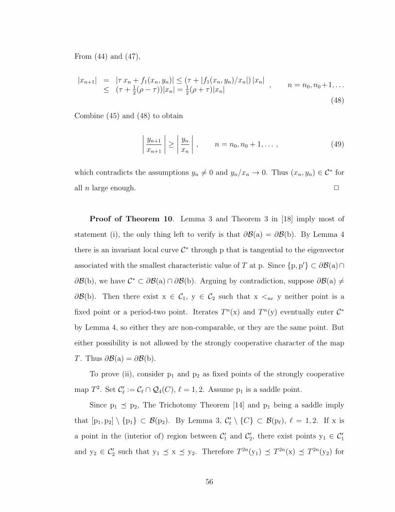


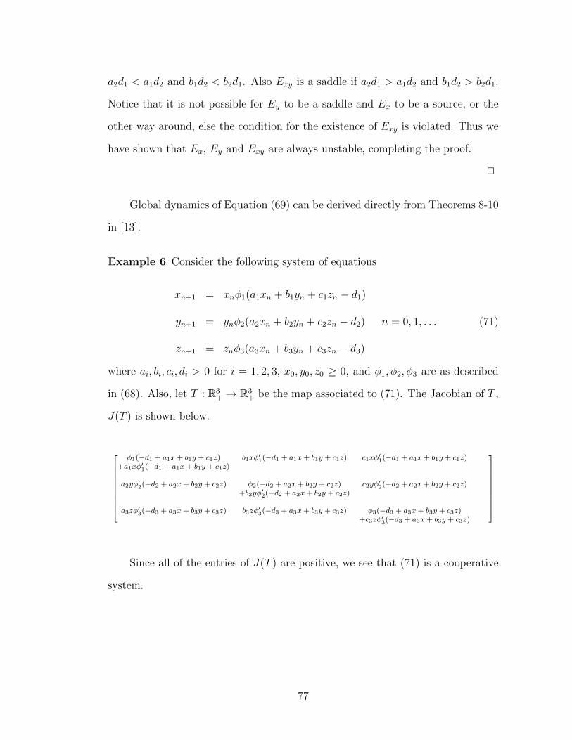


![Dualization of a Monotone Boolean Function · Monotone separable inequalities where, monotone & P-computable Th [Boros, Elbassioni, Gurvich, Khachiyan, Makino, 03] All minimal integral](https://static.documents.pub/doc/80x56/5f85d9e5a3ab42653e78ea84/dualization-of-a-monotone-boolean-function-monotone-separable-inequalities-whereioe.jpg)


