Air Force Institute of Technology Air Force Institute of Technology

AFIT Scholar AFIT Scholar

Theses and Dissertations Student Graduate Works

3-2020

Global Gradient-Based Phase Unwrapping Algorithm for Increased Global Gradient-Based Phase Unwrapping Algorithm for Increased

Performance in Wavefront Sensing Performance in Wavefront Sensing

Bryan R. Bartelt

Follow this and additional works at: https://scholar.afit.edu/etd

Part of the Optics Commons, and the Theory and Algorithms Commons

Recommended Citation Recommended Citation Bartelt, Bryan R., "Global Gradient-Based Phase Unwrapping Algorithm for Increased Performance in Wavefront Sensing" (2020). Theses and Dissertations. 4328. https://scholar.afit.edu/etd/4328

This Thesis is brought to you for free and open access by the Student Graduate Works at AFIT Scholar. It has been accepted for inclusion in Theses and Dissertations by an authorized administrator of AFIT Scholar. For more information, please contact richard.mansfield@afit.edu.

GLOBAL GRADIENT-BASED PHASE UNWRAPPING ALGORITHM

FOR INCREASED PERFORMANCE IN WAVEFRONT SENSING

THESIS

Bryan R. Bartelt, Captain, USAF

AFIT-ENG-MS-20-M-006

DEPARTMENT OF THE AIR FORCE AIR UNIVERSITY

AIR FORCE INSTITUTE OF TECHNOLOGY

Wright-Patterson Air Force Base, Ohio

DISTRIBUTION STATEMENT A.

APPROVED FOR PUBLIC RELEASE; DISTRIBUTION UNLIMITED.

The views expressed in this document are those of the author and do not reflect the

official policy or position of the United States Air Force, the United States Department of

Defense, or the United States Government. This material is declared a work of the U.S.

Government and is not subject to copyright protection in the United States.

AFIT-ENG-MS-20-M-006

GLOBAL GRADIENT-BASED PHASE UNWRAPPING ALGORITHM

FOR INCREASED PERFORMANCE IN WAVEFRONT SENSING

THESIS

Presented to the Faculty

Department of Electrical and Computer Engineering

Graduate School of Engineering and Management

Air Force Institute of Technology

Air University

Air Education and Training Command

In Partial Fulfillment of the Requirements for the

Degree of Master of Science in Electrical Engineering

Bryan R. Bartelt, B.S.E.E.

Captain, USAF

26 March 2020

DISTRIBUTION STATEMENT A

APPROVED FOR PUBLIC RELEASE; DISTRIBUTION UNLIMITED

AFIT-ENG-MS-20-M-006

GLOBAL GRADIENT-BASED PHASE UNWRAPPING ALGORITHM

FOR INCREASED PERFORMANCE IN WAVEFRONT SENSING

THESIS

Bryan R. Bartelt, B.S.E.E.

Captain, USAF

Committee Membership:

Stephen C. Cain, PhD

Chair

Maj David Becker, PhD

Member

Capt Joseph Tompkins, MS

Member

iv

AFIT-ENG-MS-20-M-006

Abstract

As the reliance on satellite data for military and commercial use

increases, more effort must be exerted to protect our space-based assets. In

order to help increase our space domain awareness (SDA), new approaches to

ground-based space surveillance via wavefront sensing must be adopted.

Improving phase-unwrapping algorithms in order to assist in phase retrieval

methods is one way of increasing the performance in current adaptive optics

(AO) systems.

This thesis proposes a new phase-unwrapping algorithm that uses a

global, gradient-based technique to more rapidly identify and correct for

areas of phase wrapping during particular phase retrieval methods. This is

beneficial in regard to the speed and accuracy within which a wrapped phase

estimate is unwrapped using a new algorithm, and doing so without having

to change current AO systems or physical setups.

v

Acknowledgements

I’d like to thank Dr. Cain, for his never-ending guidance and patience

throughout my research and writing process. His expertise and dedication

truly made my time at AFIT extremely fascinating, informative and

enjoyable.

I’d also like to thank my wife, for her continued support and her never-

wavering enthusiasm during my long nights and weekends of writing.

- Bryan Bartelt

vi

Table of Contents

Page

Table of Contents ................................................................................................ vi

List of Figures .................................................................................................. viii

List of Tables ...................................................................................................... xi

I. Introduction .................................................................................................. 1

1.1 Motivation ............................................................................................... 2

1.2 Wavefront Sensors ................................................................................. 3

1.3 Thesis Overview ..................................................................................... 5

II. Background ................................................................................................... 7

2.1) Essential Optics Theory ......................................................................... 7

2.1.1) Light Propagation ........................................................................... 7

2.1.2) Wave Front Construction ............................................................... 8

2.2) Phase Retrieval .................................................................................... 10

2.2.1) The Intensity Based Least Squares Method ............................... 11

2.2.2) The Electric Field Correlation Method ........................................ 12

2.2.3) The Gerchberg-Saxton Method .................................................... 13

2.2.4) Phase unwrapping ........................................................................ 15

2.2.5) Zingarelli Combined Method ........................................................ 20

III. MATLAB Simulation .............................................................................. 21

3.1) MATLAB Simulation Methodology ..................................................... 21

3.1.1) Generating Random Turbulent Phase Screens ........................... 22

3.1.2) Generating Point Spread Functions ............................................ 25

3.1.3) Testing Motivation/Objectives ...................................................... 27

3.2) Phase Unwrapping Simulation ............................................................ 28

3.2.1) Testing Procedure – Phase Unwrapping Methods ...................... 28

3.2.2) Phase Unwrapping Results .......................................................... 33

3.3) Phase Retrieval Simulations ............................................................... 38

3.3.1) Testing Procedure – Phase Retrieval Methods ........................... 39

3.3.2) Phase Retrieval Results ............................................................... 43

vii

IV. Lab Simulation ........................................................................................ 48

4.1) Lab Setup .............................................................................................. 48

4.2) Evaluation Methodology ...................................................................... 48

4.3) Results from Lab Data ......................................................................... 53

4.4) Conclusion ............................................................................................ 56

V. Conclusion ................................................................................................... 57

5.1) Thesis Conclusions ............................................................................... 57

5.2) Future Work ......................................................................................... 58

Works Cited ....................................................................................................... 59

viii

List of Figures

Page

Figure 1: An example of how WFSs and lenslets detect atmospheric

turbulence. ................................................................................................ 4

Figure 2: Phase descriptions of the first 21 Zernike polynomials ..................... 9

Figure 3: An example of a generated phase screen with discontinuity caused

by an aperture. ........................................................................................ 15

Figure 4: An example of a wrapped phase screen. ........................................... 16

Figure 5: An overhead look at the wrapped phase screen from Figure 4. ...... 16

Figure 6: An example of the K(x,y) matrix, which attempts to locate the

regions where the phase wraps and seeks to add radians back to the

wrapped phase with integer values. ...................................................... 18

Figure 7: Simulated telescope aperture. ......................................................... 22

Figure 8: Non-turbulent PSF generated from a plane wave clearly shows

perfect symmetry across the detector plane. ......................................... 26

Figure 9: Turbulent PSF on the detector plane generated from a turbulent

wavefront passing through simulated optical aperture. ....................... 27

Figure 10: Example of a wrapped phase shows the discontinuity when phase

values exceed π/- π radians. ................................................................... 29

Figure 11: GBU and LSU performance with turbulence of D/r0 = 1. ............ 35

ix

Figure 12: Close up of the GBU and LSU performance with turbulence of

D/r0 = 1. The difference of the average values between 108 Hz and 143

Hz is approximately = 0.0032, in favor of the LSU. .............................. 35

Figure 13: GBU and LSU performance with turbulence of D/r0 = 1.1. ......... 36

Figure 14: Close up of the GBU and LSU performance with turbulence of

D/r0 = 1.1. The difference of the average values between 108 Hz and

143 Hz is approximately = 0.00049, in favor of the LSU. ..................... 36

Figure 15: GBU and LSU performance with turbulence of D/r0 = 2. ............ 37

Figure 16: Close up of the GBU and LSU performance with turbulence of

D/r0 = 2. The difference of the average values between 108 Hz and 143

Hz is approximately = 0.01089, in favor of the GBU. ........................... 37

Figure 17: Noisy, wrapped phase outputted from the Gerchberg-Saxton ..... 44

Figure 18: GS-LSU Zernike difference at D/r0 = 1 greatly exceeds difference

of other phase retrieval methods. .......................................................... 44

Figure 19: GS-LSU Zernike difference at D/r0 = 2 greatly exceeds difference

of other phase retrieval methods. .......................................................... 45

Figure 20: The GS-GBU outperforms the other phase retrieval methods at all

bandwidths with D/r0 = 1. ...................................................................... 45

Figure 21: The GS-GBU outperforms the other phase retrieval methods at all

bandwidths with D/r0 = 1.5. ................................................................... 46

x

Figure 22: The GS-GBU and other phase retrieval methods have comparable

differences from 1Hz – 47Hz at D/r0 = 2. However, the IBLS and EFC

method’s max bandwidth is much smaller than that of the GS-GBU. . 46

Figure 23: The cross-sections of the collected PSFs and the theoretical PSF

given a D/r0 value of 1.515 match up nearly perfect. ........................... 49

Figure 24: Example of an altered PSF for more simplistic computations. ..... 51

Figure 25: Flowchart explaining evaluation methodology. ............................. 52

Figure 26: The groupings of Zernike polynomials given their variances as

D/r0 increases. ........................................................................................ 53

Figure 27: The means of the estimated Zernike coefficients derived from the

GS-GBU and GS-LSU phase retrieval techniques. ............................... 54

Figure 28: The GS-GBU variances are much more realistic to the theoretical

by slightly exceeding them. The GS-LSU variances are much lower

than should be expected. ........................................................................ 55

xi

List of Tables

Page

Table 1: Average iteration time for phase unwrappers……………………….. 31

Table 2: Rate at which generated wavefronts exceed tilt constraint……….. 34

Table 3: Average iteration time for phase retrieval methods………………... 41

Table 4: Max iterations the phase retrieval methods can execute/second…. 42

Equation Section (Next)

1

GLOBAL GRADIENT-BASED PHASE UNWRAPPING

ALGORITHM FOR INCREASED PERFORMANCE IN

WAVEFRONT SENSING

I. Introduction

On December 20, 2019, the United States Space Force was stood up in

order to protect US and allied assets and ensure the peaceful use of space for

all responsible actors, consistent with applicable law, including international

law [1]. In order to achieve this mission, the ability to thoroughly survey all

commercial, friendly and hostile space material is of utmost importance.

Using ground-based imaging systems are among the most cost-effective and

convenient ways to ensure the Space Force maintains its Space Domain

Awareness (SDA). These imaging systems are vital to the detection and

surveillance of known and unknown space objects in Geosynchronous, Low-

Earth and Highly Elliptical orbits, as well as objects passing near to the

earth.

There are three main areas of concern in space for the continued

safeguarding of US assets and the Earth: space debris, micro-satellites and

near-earth asteroids (NEAs) [2, 3, 4]. These all pose a threat to the earth and

satellite networks that perform communication, security and research

objectives for many public, private and state-run organizations, including the

US Space Force and the US Department of Defense. In an already clustered

2

space environment where the number of all three of these threats are

increasingly being detected, ground-based optical systems must continue to

adapt new and improved image registration techniques that can account for

the optical turbulence caused by the Earth’s atmosphere.

1.1 Motivation

This thesis aims to explore a common ground-based image restoration

method that compensates for phase aberrations due to atmospheric

turbulence. This common method is to be implemented in wavefront sensors

(WFS) in order to improve the quality of images collected. The theoretical

method should work independently of an optical system’s physical attributes,

and solely seek to update and inform the system’s WFS as quickly and

accurately as possible.

These image restoration methods that attempt to counter atmospheric

turbulence can be called phase retrieval. In mathematical terms, phase

retrieval is described as recovering a complex signal, given only the

magnitude-squared of its Fourier transform. This means that phase retrieval

methods attempt to estimate the phase of a complex signal without any

initial phase information given. This concept is used for many different signal

and image processing problems.

However, unlike some other applications, when used in conjunction

with telescope optics, information about the imaging system can also be

included. This extra information includes the physical properties of the

3

imaging system and can help recover a better estimate of the unknown

phase.

Phase retrieval methods used in telescopes and WFS’s attempt to

recover the unknown phase value from a wavefront that is incident to the

system’s aperture given only the intensity data, 𝐼𝑑(𝑥′, 𝑦′), in the detector

plane. See Equations (1.1) & (1.2), where taking the Fourier Transform of

𝐴(𝑥, 𝑦), which is a mathematical 2-D representation of the aperture’s shape

and size, and 𝜃(𝑥, 𝑦), which is the unknown turbulent wavefront, results in

the complex field in the detector plane, 𝐻𝑑(𝑥′, 𝑦′).

2( ', ') | ( ', ') |d dI x y H x y= (1.1)

( ( , ))( ', ') ( , ) j x y

dH x y F A x y e −= (1.2)

In the effort to try and recover the unknown phase value, the

estimated phase screens can become “wrapped” due to the limitations in both

hardware and software. This is another hurdle that will be explored in this

thesis.

1.2 Wavefront Sensors

Resolving an image of a space-based object from a ground-based

imaging system can prove difficult when atmospheric turbulence is present.

Wavefront sensors, which aim to counter the effects of atmospheric

turbulence, sometimes need to operate around the millisecond level. This

4

ensures that the aberrations in the image can be measured and accounted for

prior to the wavefront distorting the image further.

Common wavefront sensors, like the Shack-Hartmann WFS, consist of

an array of small, identical lenses, called lenslets. When a plane wave is

incident to the telescope pupil, these lenslets divide the light entering the

aperture into sub-apertures that project the image onto a CCD at positions

determined by the array’s geometry. When the incident wave has been

disrupted by the atmosphere, the images projected by the lenslets will no

longer fall on the CCD in geometric fashion (See Figure 1). These

displacement measurements are passed on to the other adaptive optics (AO)

components and are used to account for the tilt aberrations caused by the

atmosphere over each sub-aperture. Local tilt information can be used to

reconstruct the wave front over the entire aperture.

Figure 1: An example of how WFSs and lenslets detect atmospheric turbulence [5].

5

1.3 Thesis Overview

Exploring new phase unwrapping and phase retrieval methods will

bolster the ability of ground-based telescopes to resolve and refine images

taken through the atmosphere. This will increase the detection rates for

space debris, micro-satellites and NEAs, resulting in more comprehensive

SDA.

Chapter II lays the foundation with background information and

assumptions needed to explore the concept of phase unwrapping and phase

retrieval. Several existing phase retrieval methods, as well as related

research are introduced to establish a baseline of knowledge for the reader.

The new phase unwrapping approach is also examined.

Chapter III motivates the reader and outlines the materials and

process used for simulation and comparison of the aforementioned phase

unwrappers and phase retrieval methods. This chapter also analyzes the

results from simulation, as the next chapter will examine the concepts with

real world lab data.

Chapter IV dives into the feasibility of the phase unwrapping and

phase retrieval methods by using collected lab data to evaluate and compared

methods. The materials and process used for data collection and evaluation

are discussed, as well as the results of the evaluation.

6

Chapter V concludes the thesis with a summary of takeaways from the

comparisons of phase retrieval methods. Potential for future work is also

discussed.

Equation Section (Next)

7

II. Background

As mentioned in Chapter 1, the method of phase retrieval is an

extremely complex concept that has yet to be fully mastered or implemented

to its fullest potential. This chapter covers the basic optical theory behind the

phase retrieval problem and explores a few of the current methods that are

used in detail.

2.1) Essential Optics Theory

This thesis builds upon many fundamentals of Fourier optics derived

by Joseph Goodman [6]. Relevant subject matter includes the understanding

of light propagation through wave-optics.

2.1.1) Light Propagation

It is well known that the propagation of light to a given location can be

mathematically described using 2-D Fourier Transforms. In this thesis it is

assumed that the light source being imaged by the ground-based telescope is

normalized and far enough away to be considered a point source, with its

phase, 𝜔(𝑥, 𝑦), described as a plane wave. These assumptions also satisfy the

Fraunhofer propagation criteria [6]. Once the wavefront comes into contact

with the Earth’s atmosphere, it inherits an unknown phase delay, 𝜃(𝑥, 𝑦),

which distorts the light incident to the telescope’s aperture, 𝐴(𝑥, 𝑦). The

phase delay is caused due to the “boiling effect” or churning and fluctuation

in the density of the atmosphere [7]. Assuming the telescope is properly

8

focused on this normalized light source, and that 𝜔(𝑥, 𝑦) is a plane wave, the

pupil function, 𝑃(𝑥, 𝑦), at the aperture of the telescope can be expressed as:

( ( , ) ( , ))( , ) j x y x yP x y e − += (2.1)

( , )( , ) ( , ) j x yP x y A x y e −= (2.2)

Propagating from the pupil plane to the telescope’s detector plane can

be mathematically expressed using a Fourier Transform, where ( , )x y are

coordinates in the pupil plane and ( ', ')x y are coordinates in detector plane.

Taking the magnitude squared of this propagation gives us the measured

intensity, 𝐼𝑑(𝑥′, 𝑦′), on the detector plane.

2( ', ') | { ( , )} |dI x y F P x y= (2.3)

This intensity pattern is the measured data that is of most interest to

observers but is often distorted due to the phase delay, 𝜃(𝑥, 𝑦), caused by the

atmosphere. Throughout this paper, the Lens Maker’s equation is considered

satisfied, which implies that there are no additional focus aberrations

inherent to the intensity measurement.

2.1.2) Wave Front Construction

Expressing light’s phase using Zernike polynomials is a common way

to quantify the turbulence that the wave fronts acquire while traveling

through the atmosphere. They are an orthogonal set of polynomials used to

parameterize specific phase aberrations and carry coefficients to weight each

9

respective type of aberration. Figure 2 shows the aberration types that

Zernike polynomials describe like piston, tilt, focus, astigmatism, coma, and

more.

Figure 2: Phase descriptions of the first 21 Zernike polynomials [8].

Due to their orthogonality, these polynomials, 𝜙𝑛(𝑥, 𝑦), and their

respective coefficients, 𝑧𝑛, can be summed together to create a simulated

phase screen, 𝜃(𝑥, 𝑦). See Equation (2.4) below.

1

( , ) ( , )N

n n

n

x y z x y =

= (2.4)

All of the phase screens in this thesis do not include piston error, or 𝑧1,

as this is a term for delay and does not affect the shape of the wavefront.

10

As shown above, it is easy to see how a wavefront can be constructed

using Zernike coefficients, but in some instances, it is important to know how

to derive Zernike coefficients given only a wavefront, 𝜃(𝑥, 𝑦). This is done

using a decomposition of the wavefront into coefficients as shown below.

2

( , ) ( , )

( , )

n

x y

n

n

x y

x y x y

zx y

=

(2.5)

The comprehension of both Zernike polynomials and basic light

propagation are crucial in the understanding of imaging systems, wavefront

sensors, and the motivation behind phase retrieval.

2.2) Phase Retrieval

As stated in Section 1.1, phase retrieval is the attempt to reconstruct

the complex wavefront of a light source given only the measurement of its

intensity. It is a technique used in ground-based imaging systems that drive

optical components to account for atmospheric turbulence, helping to create a

more resolute image in the detector plane. Mathematically, phase retrieval

can be expressed as in Equation (2.6). Where 𝜃(𝑥, 𝑦) is the phase attempting

to be recovered given 𝐼𝑑(𝑥′, 𝑦′).

( , ) 2( ', ') | { ( , ) } |j x y

dI x y F A x y e −= (2.6)

The following phase retrieval methods seek to reconstruct 𝜃(𝑥, 𝑦) using

iterative or gradient based approaches with a focus in Zernike polynomials.

11

2.2.1) The Intensity Based Least Squares Method

This phase retrieval method is a gradient decent method that seeks to

determine the value of Zernike coefficients that best model the true phase

using an iterative sum of squared errors comparison of the measured PSF

and estimated PSF [9]. The process begins by choosing a step size, Δ, and a

guess phase, 𝜃𝑖(𝑥, 𝑦), built from a set of N Zernike coefficients. Next, new

estimation wavefronts are created by altering each Zernike coefficient, one at

a time by +Δ and -Δ. This results in 2N new wavefronts, each one differencing

positively and negatively by Δ. We will call this process of altering Zernike

coefficients by Δ, ‘stepping,’ and 𝑊 will represent an array of the newly

constructed wavefronts.

2 2

2 2

3 3

3 3

( , )

( , )

( , )

( , )

( , )

( , )

i

i

i

i

N i N

N i N

x y

x y

x y

W x y

x y

x y

+

−

+

−

+

−

= +

= − = +

= = −

= + = −

(2.7)

Once the new wavefronts are produced, their intensity’s can be

computed using Equation (2.6). The 2N newly estimated intensity models can

then be compared to the true measured PSF. The resulting comparison that

yields the minimum sum of squared error passes on their respective Zernike

coefficients that become the new guessed wavefront, 𝜃𝑖(𝑥, 𝑦), for the next

iteration of the Intensity Based Least Squares (IBLS) method. Below, the

12

comparisons between the PSFs are calculated where 𝐼𝑑(𝑥′, 𝑦′) is the true,

measured PSF, and 𝐼𝑊(𝑥′, 𝑦′) is each estimated PSF and WQ is the sum

squared error associated between the two.

2ˆ[ ( ', ') ( ', ')]W d W

x y

Q I x y I x y= − (2.8)

This iterative process is continued until a maximum amount of

iterations has been met, or WQ breaks an error threshold, producing an

estimate of the true waveform through Zernike coefficients. It is worth

mentioning that this method performs better if something is already known

about the incident phase screen and its respective Zernike coefficients prior

to the first iteration.

2.2.2) The Electric Field Correlation Method

There is another phase retrieval method that uses Zernike coefficient

stepping and estimation but instead uses the estimate electric-field in the

detector plane. Similar to the IBLS, the Electric-Field Correlation (EFC)

method evaluates a model of the system’s E-field, and a set of altered,

Zernike-weighted E-fields. The initial E-field model, ˆ ( ', ')H x y , is calculated by

propagating a given, user-chosen, input phase derived from Zernike

coefficients, 𝜃𝑖(𝑥, 𝑦), through the known aperture of the optical system.

( , )ˆ ( ', ') { ( , ) }ij x yH x y F A x y e

−= (2.9)

13

Similar to the IBLS algorithm, this technique produces estimation

wavefronts by altering N Zernike coefficients by a pre-determined step size,

Δ. Next a comparison of the 2N estimated electric fields, 𝐻𝑤(𝑥′, 𝑦′), versus the

modeled electric field, ��(𝑥′, 𝑦′) is calculated by seeing how correlated they

are.

ˆ ( ', '), ( ', ')*

ˆ( ( ', '), ( ', '))ˆ ˆ( ', ') ( ', ')* ( ', ') ( ', ')*

W

x y

W W

W W

x y x y

H x y H x y

H x y H x yH x y H x y H x y H x y

=

(2.10)

The estimated electric field with the highest correlation value, W , will

have its respective Zernike coefficients used to build the input wavefront for

the next iteration. Like the IBLS method, this iterative process is continued

until a maximum amount of iterations has been met, orW breaks a

threshold, producing an estimate of the true Zernike coefficients and

inherently an estimate of the true waveform. It is worth mentioning that this

method performs better if something is already known about the incident

phase screen and its respective Zernike coefficients prior to the first iteration.

2.2.3) The Gerchberg-Saxton Method

Another common phase retrieval method was conceived by R.W.

Gerchberg and W.O. Saxton in the 1980’s [10]. This iterative method begins

14

with the known intensity measurement, the aperture’s physical

characteristics and a guess at the wavefront adherent to the aperture.

Gerchberg and Saxton used simple Fourier optics to propagate and

reverse-propagate the wavefront back and forth from the detector plane to

the aperture plane ensuring that the true aperture, 𝐴(𝑥, 𝑦), and measured

intensity, 𝐼𝑑, are inputted before each propagation, while the phase value is

left to fluctuate. This can be shown in the 4 steps below.

1 ( ', ') ( , )

( , ) ( , )

( , ) ( ', ')

( ', ') ( ', ')

ˆ{ ( ', ') } ( , )

( , ) ( , )

{ ( , ) } ( ', ')

ˆ( ', ') ( ', ')

j x y j x y

d

j x y j x y

j x y j x y

d

j x y j x y

d d

F I x y e A x y e

A x y e A x y e

F A x y e I x y e

I x y e I x y e

− − −

− −

− −

− −

=

→

=

→

(2.11)

This method can eventually lead to the phase converging closely to

what the original incident phase screen looked like if the first guessed phase

was chosen wisely. A parabolic wavefront of any type is usually a good choice

for the guess input phase.

An issue with this method is that it outputs a wrapped phase. Phases

are wrapped when the phase exceeds values of -π or π radians, which results

in the algorithm losing track of how many radians the phase has spanned.

This can happen with turbulent wavefronts and the more iterations of

Gerchberg-Saxton that are executed, the more wrapped the phase becomes.

15

2.2.4) Phase unwrapping

As discussed, the Gerchberg-Saxton phase retrieval method concludes

with a wrapped phase, where all values are constrained between -π and π

radians. This is a common problem among other optical devices and

algorithms, where the surpassing of 360 degrees cannot be accounted for due

to excess noise, discontinuities or software limitations. Currently one of the

industry standards for phase unwrapping, and one of the techniques that will

be explored further in this paper, is the Calibrated Phase Unwrapping based

on Least-Squares and Iterations (CPULSI) [11]. Although it excels with

generic noisy wrapped phases, its performance seems to depreciate when

there are moments of discontinuity across the wavefronts from places like a

telescope aperture. See Figure 3 below. This technique will be referred to in

this paper as the Least Squares Unwrapper (LSU).

Figure 3: An example of a generated phase screen with discontinuity caused by an aperture.

16

Figure 4: An example of a generated wrapped phase screen.

Figure 5: An overhead look at the wrapped phase screen from Figure 4.

17

The proposed phase unwrapping technique attempts to unwrap phase

screens with large amounts of noise, as well as more effectively account for

moments of discontinuity. This iterative, gradient-based approach will

theoretically unwrap phase screens more quickly and more accurately given

optical systems that have places of discontinuity. This method will be

referred to as the Gradient-Based Unwrapper (GBU). To begin, it can be

helpful to think about a wrapped phase as in Equation (2.12) below, where

( , )K x y is a matrix consisting of negative and non-negative integer values,

( , )x y is a turbulent phase screen, and ( , )x y is its wrapped phase.

( , ) ( , ) 2 ( , )x y x y K x y = + (2.12)

Figure 6: Wrapped phases are true phases that have exceeded a threshold of +/- 2 radians.

The ( , )K x y matrix attempts to locate the moments where the phase is

wrapped, and to add or subtract the lost amounts of 2 radians of delay

across phase screen. Note: in the first iteration of the GBU, the ( , )K x y

matrix is initially set to zero.

18

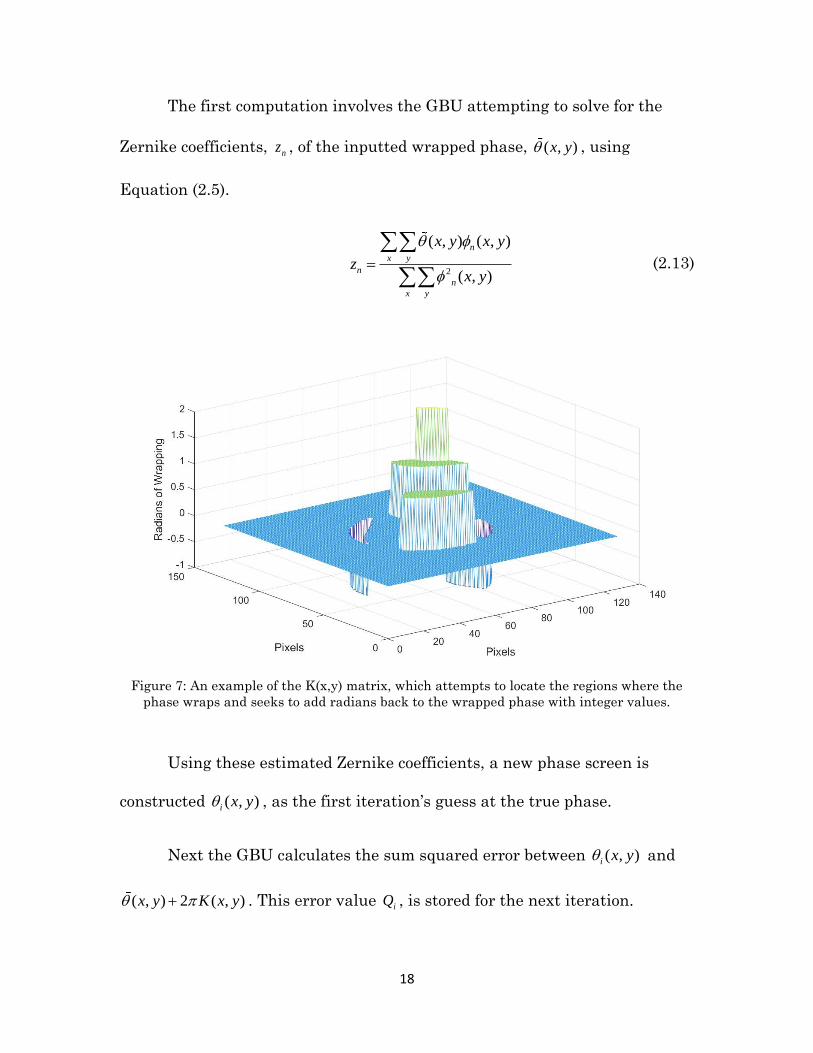
The first computation involves the GBU attempting to solve for the

Zernike coefficients, nz , of the inputted wrapped phase, ( , )x y , using

Equation (2.5).

2

( , ) ( , )

( , )

n

x y

n

n

x y

x y x y

zx y

=

(2.13)

Figure 7: An example of the K(x,y) matrix, which attempts to locate the regions where the

phase wraps and seeks to add radians back to the wrapped phase with integer values.

Using these estimated Zernike coefficients, a new phase screen is

constructed ( , )i x y , as the first iteration’s guess at the true phase.

Next the GBU calculates the sum squared error between ( , )i x y and

( , ) 2 ( , )x y K x y + . This error value iQ , is stored for the next iteration.

19

( )2

( , ) ( , ) 2 ( , )i i

x y

Q x y x y K x y = − − (2.14)

Next, the gradient of the difference between ( , )i x y and ( , )x y in

respect to ( , )K x y is evaluated to identify the moments of wrapping.

( )0 0

0 0 0 0

( , )4 ( , ) ( , ) 2 ( , )

( , ) ( , )x y

dQ dK x yx y x y K x y

dK x y dK x y

= − − −

(2.15)

( )0 0 0 0

0 0

4 ( , ) ( , ) 2 ( , )( , )

dQx y x y K x y

dK x y = − − − (2.16)

The moments where the gradient exceeds the threshold correspond to

the regions where ( , )K x y will be increased or decreased by one.

0 0

0 0

0 0

0 0

0 0

if ( , ) 1( , )

( , ) if ( , ) 1( , )

Otherwise ( , ) 0

i

i

dQK x y

dK x y

dQK x y K x y

dK x y

K x y

− = −

= = =

(2.17)

Once ( , )K x y is revised with the logic above, the iteration is complete.

( , )K x y and ( , )i x y are then passed onto the next iteration. The algorithm is

considered converged when the difference between the error values of

consecutive iterations, iQ and 1iQ − are lessened to beat a user defined

threshold. This infers that the algorithm could not find any other regions to

compensate for lost radians in the wrapped phase.

20

2.2.5) Zingarelli Combined Method

Unfortunately, gradient decent methods, like the IBLS, often get

trapped in local minima [9]. Others, like Zingarelli, have attempted to avoid

problems like this by combining techniques. Zingarelli’s resulting method

involves the IBLS and EFC algorithms, plus the Gerchberg-Saxton phase

retrieval method.

Using the intensity measurement, Zingarelli first estimates the E-field

through an iteration of the Gerchberg-Saxton method in order to retrieve

estimated Zernike coefficients from the EFC method. Once the Zernike

coefficients are estimated, they become the initial conditions for the IBLS

method.

The output of the IBLS method produces Zernike coefficients as well

that create a phase that is checked against a error threshold. If this threshold

is not breached, then the phase is used as the input guess for another

iteration of the GS algorithm, which initiates another iteration of the whole

process.

This method has been shown to improve the accuracy for phase

retrieval problems, but its speed and feasibility in wavefront sensors have not

been tested.

Equation Section (Next)

21

III. MATLAB Simulation

In this chapter, MATLAB R2018a was used to test, evaluate and

compare the different phase retrieval methods to the proposed method. The

computer used to perform this simulation possessed an 8th generation, i7 core

processor. For both situations the impulse responses of the telescope, or in an

optical system’s case: the Point Spread Functions (PSFs), were generated

with known waveform aberrations. These aberrations are known to the

observers but are not passed on to the phase retrieval methods as any sort of

initial parameter and will have no effect on the performance of any of the

methods.

Another condition of the simulation is that each PSF was measured

independently in time to all other PSFs. Therefore, this simulation is

theoretically built to evaluate completely independent short exposure frames

of an optical system (>20ms). The wavelength of the light theoretically does

not matter, meaning that the following techniques could be used in any

imaging system for any region of the electromagnetic spectrum.

3.1) MATLAB Simulation Methodology

The MATLAB simulations rely upon creating PSFs using a

mathematical representation of an optical system’s physical features, as well

as the using the generation of turbulent, statistically independent,

wavefronts.

22

The particular scenario being looked at for the following simulations

are that of an optical system undergoing an attempt to image a single star,

given an arbitrary wavelength, from Earth’s surface. The star in question is

far enough away from Earth to be considered a perfect point source. The

resulting PSFs, phase screens and optical system aperture are all expressed

via 128x128 pixel matrices, with the circular pupil of the aperture having a

diameter of 64 pixels. This leaves an area of discontinuity across the aperture

like a true telescope as shown in Figure 7.

Figure 8: Simulated telescope aperture.

3.1.1) Generating Random Turbulent Phase Screens

First, the turbulent phase screen is calculated based on a finite set of

Zernike polynomials with coefficients, 𝑧𝑛. This set of coefficients, 𝑍→

, will

represent the random atmospheric aberrations to the simulated optical

system: focus, astigmatism, coma, etc.

23

1

2

n

z

zZ

z

=

(3.1)

In order to build a realistic phase screen, we need to account for the

Zernike Coefficient’s covariance. According to Roddier [12], a spectral

decomposition of the coefficients is required. This is achieved by using a

Cholesky Factorization effort once the coefficient’s covariance matrix is

found.

Using Noll’s derivation given that the Zernike coefficients are

Gaussian random variables, with zero mean, the resulting covariance matrix,

𝐶, for the Zernike coefficients is given below [13].

0.4536 0 0 0 0 0 0.0143 0 0 0

0 0.4536 0 0 0 0.0143 0 0 0 0

0 0 0.0235 0 0 0 0 0 0 0.0039

0 0 0 0.0235 0 0 0 0 0 0

0 0 0 0 0.0235 0 0 0 0 0

0 0.0143 0 0 0 0.0063 0 0 0 0

0.0143 0 0 0 0 0 0.0063 0 0 0

0 0 0 0 0 0 0 0.0063 0 0

0 0 0 0 0 0 0 0 0.0063 0

0 0 0.0039 0 0 0 0 0 0 0.0025

C

−

− −

= −

−

−

(3.2)

These values theoretically make sense because we know that the lower

order Zernike polynomials carry more of the phase screen’s error. Luckily,

wave front sensors are able to automatically adjust for the tilt coefficients, 𝑧2

and 𝑧3. This is achieved by the sensor automatically tracking the PSF across

24

the detector plane using a center of mass technique. This infers that the tilt

coefficients can be ignored, and the algorithms can focus solely on estimating

the higher order Zernike’s (𝑧4 and higher), and not have to worry about the

position of the PSF.

Next, the overall magnitude of 𝐶 also changes depending on the

relationship between the diameter of the system’s aperture, 𝐷, and the Fried

parameter, 𝑟0, which is a scalar measurement of the quality of optical

transmission through the atmosphere.

The ratio of 𝐷/𝑟0 has a direct effect on the magnitude of turbulence

seen in the generated waveform, and therefore a direct effect on the resulting

noise seen in the PSF. In order to mitigate the effects of the atmosphere,

most wave front sensors are designed with the average Fried parameter

value of the surrounding environment in mind. This keeps the ratio of 𝐷/𝑟0 as

close to 1 as possible as often as possible. The resulting equation, based on

coefficients 𝑧4 through 𝑧11, is computed to be:

(5/3)

0.0235 0 0 0 0 0 0 0.0039

0 0.0235 0 0 0 0 0 0

0 0 0.0235 0 0 0 0 0

0 0 0 0.0063 0 0 0 0

0 0 0 0 0.0063 0 0 0

0 0 0 0 0 0.0063 0 0

0 0 0 0 0 0 0.0063 0

0.0039 0 0 0 0 0 0 0.00

0

25

DC

r

−

= −

(3.3)

25

Then, the result of a Cholesky factorization of the covariance matrix,

𝑊, can be used to calculate a set of true Zernike coefficients, ��, using the

following formula [12]. Where 𝑛→

is a set of Gaussian random variables with

zero mean and unit variance.

TC WW= (3.4)

Z nW= (3.5)

Now we are able to accurately depict a distorted wavefront due to

atmospheric optical aberrations. The resulting randomly generated phase

screen, 𝜃(𝑥, 𝑦), is computed using a sum of the products of the true aberration

values, 𝑧𝑛

^, and their respective Zernike polynomials, 𝜙𝑛(𝑥, 𝑦).

11

4

ˆ ˆ( , ) ( , )n n

n

x y z x y =

= (3.6)

Note that the covariance values in 𝐶 are subject to change if the

Zernike coefficient’s variances are altered.

3.1.2) Generating Point Spread Functions

Next, the physical characteristics of the optical system’s aperture,

𝐴(𝑥, 𝑦), are considered and mathematically described (usually as a rect or circ

function) and multiplied with the incident waveform’s complex field as show

below to produce the system’s pupil function, 𝑃(𝑥, 𝑦).

ˆ( , )( , ) ( , ) j x yP x y A x y e −= (3.7)

26

Finally, we can produce the simulated PSF, 𝐼𝑑(𝑥′, 𝑦′), by taking the

magnitude and square of the two-dimensional Fourier transform of the pupil

function [6]. The PSF is the only bit of information known to the observer and

is the only bit of measured data passed to the phase retrieval algorithms.

2ˆ ( ', ') ( , )dI x y F P x y= (3.8)

An example of what a non-turbulent PSF, where 𝜃(𝑥, 𝑦) is a plane

wave, and therefore has Zernike coefficient values equal to 0, would look like

is shown below in Figure 8. Assume 𝐷/𝑟0 = 1.

Figure 9: Non-turbulent PSF generated from a plane wave clearly shows perfect symmetry

across the detector plane.

Comparatively, a turbulent PSF is shown in Figure 9. It is the result of

aberrations in the respective wave front caused from atmospheric turbulence.

In other words, its Zernike coefficients ≠ 0.

27

Figure 10: Turbulent PSF on the detector plane generated from a turbulent wavefront

passing through simulated optical aperture.

3.1.3) Testing Motivation/Objectives

Understanding the primary focus for comparison of these phase

unwrapping and phase retrieval methods is to understand how well they

perform when implemented into an AO system. AO systems rely on making

small adjustments to their components within milliseconds to measure and

adapt to atmospheric turbulence. That is why this simulation will look to

evaluate these methods based off of their speed, as well as their accuracy.

This is in order to realistically evaluate the algorithms as if they were

employed in a true WFS, where the atmosphere is changing on a millisecond

timescale [5]. Concerning the accuracy of these algorithms, the sum squared

error of the estimated phase screens with the true phase screen will be

calculated once the resulting time restraint given by the AO system is

expired, or when the algorithm has converged to an estimate.

Several of the phase retrieval methods use Zernike coefficients to

generate their estimated wave fronts, which can then be used as another

accuracy metric. As explained in Section 2.1.2 an existing wavefront can use

28

the inverse tactic and use the Zernike decomposition technique using

Equation (2.5) to produce a set of coefficients based on a measured phase

screen. Simply put, the difference between the sets of true Zernike

coefficients and estimated coefficients become data that can also be compared

for accuracy.

For the purpose of this simulation, the effectiveness of the two phase

unwrappers will be assessed first. This will serve as a good segway and

support piece to the phase retrieval evaluations to follow.

3.2) Phase Unwrapping Simulation

As stated prior, phase unwrapping methods are very important to

phase retrieval methods and AO systems in general. Optical components and

even phase retrieval methods like Gerchberg-Saxton can leave a system stuck

with trying to unwrap a phase screen. Therefore, it is worth exploring and

comparing the effectiveness of the LSU versus the GBU.

In order to simulate how well the LSU and GBU would theoretically

work in an AO system, they will be tested to see how accurately and timely

they can unwrap and converge to a true phase screen at different 𝐷/𝑟0 values

and different operating bandwidths.

3.2.1) Testing Procedure – Phase Unwrapping Methods

For the process of evaluating the phase unwrappers, phase screens

with atmospheric noise are generated via Equations (3.3) through (3.6) using

29

𝐷/𝑟0 values between 0.7 and 2. This generates a true set of Zernike

coefficients, ��, and a resulting true phase screen, 𝜃(𝑥, 𝑦). In order to ensure

most of the wavefronts that are being passed to the algorithms are wrapped

wavefronts, a random piston value is added to the phase screen. The piston

value, η, will be uniformly distributed between -π and π. Next, the phase

angle of the true wavefront’s field is calculated in order to produce a wrapped

phase, ��(𝑥, 𝑦).

ˆ( ( , ) )( , ) j x yx y e − += (3.9)

Figure 11: Example of a wrapped phase shows the discontinuity when phase values exceed

π/- π radians.

This wrapped phase is one of two common inputs needed to compare

the LSU and GBU. The other common input is the error threshold, ε.

Between each iteration of the trial, the unwrappers will check if the absolute

difference between the current iteration, 𝑖𝑛, and previous iteration’s

estimated unwrapped phase screen has changed less than ε. The arbitrary

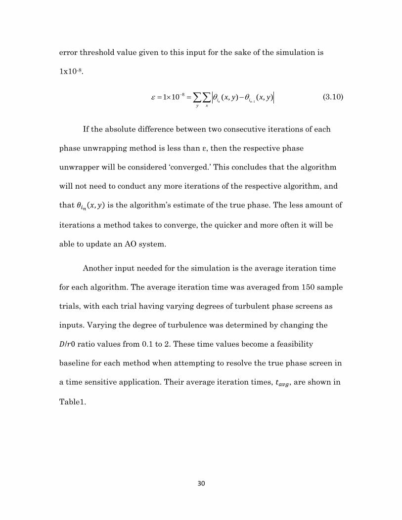
30

error threshold value given to this input for the sake of the simulation is

1x10-8.

1

81 10 ( , ) ( , )n ni i

y x

x y x y −

−= = − (3.10)

If the absolute difference between two consecutive iterations of each

phase unwrapping method is less than ε, then the respective phase

unwrapper will be considered ‘converged.’ This concludes that the algorithm

will not need to conduct any more iterations of the respective algorithm, and

that 𝜃𝑖𝑛(𝑥, 𝑦) is the algorithm’s estimate of the true phase. The less amount of

iterations a method takes to converge, the quicker and more often it will be

able to update an AO system.

Another input needed for the simulation is the average iteration time

for each algorithm. The average iteration time was averaged from 150 sample

trials, with each trial having varying degrees of turbulent phase screens as

inputs. Varying the degree of turbulence was determined by changing the

𝐷/𝑟0 ratio values from 0.1 to 2. These time values become a feasibility

baseline for each method when attempting to resolve the true phase screen in

a time sensitive application. Their average iteration times, 𝑡𝑎𝑣𝑔, are shown in

Table1.

31

Phase Unwrapping Method Iteration Time (sec/iteration), 𝒕𝒂𝒗𝒈

Least Squares Unwrapper 0.00233

Gradient Based Unwrapper 0.00231

Table 1: Average iteration time for phase unwrappers.

Using these time values, one can calculate on average how many

iterations can be accomplished in a trial. Given an AO system’s operating

bandwidth, 𝑏𝑤, the maximum amount of iterations a method can manage in a

trial of the simulation, 𝑖max, is simply:

max

1

avg

ibw t

=

(3.11)

These bandwidths will reflect certain operating speeds that AO

system’s physical components can operate at. In order to capture enough data

to be statistically sound, the operating bandwidths will be increased from

1Hz to 300Hz, evaluating a set of 300 different wrapped phases at each

observed bandwidth value. The 𝐷/𝑟0 value will be varied to particular values

of interest.

In each trial, a random, yet true, phase screen is built from its

respective Zernike coefficients. Each phase unwrapping method will attempt

to resolve the true phase screen with only their respective 𝑖max values. Once

the unwrappers converge or hit their iteration limit, each method will have

produced a guess-phase screen, 𝜃method(𝑥, 𝑦), that attempts to depict the true

phase screen value, 𝜃(𝑥, 𝑦). A set of estimated Zernike coefficient values,

32

��method, can then be decomposed from the estimated phase screen. See

Equation (2.5).

This guess-phase screen is the main output of the LSU and GBU

algorithms, as they have attempted to reconstruct the complex waveform that

was incident to the optical system’s aperture given a measured PSF.

The following metrics aim to evaluate and compare the Least Squares

Unwrapper against the Gradient Based Unwrapper’s accuracy and their

feasibility for use in an AO system.

1. The sum of the absolute differences between true and estimated

Zernike coefficients.

𝑧𝑒𝑟𝑛_𝑒𝑟𝑟𝑚𝑒𝑡ℎ𝑜𝑑 = ∑ |��𝑛 − ��𝑛|

𝑛

2. Evaluate the algorithms at different bandwidths and different

𝐷/𝑟0 values.

Metric 1 has one stipulation: During the decomposition from the phase

screen into Zernike coefficients, both the GBU and LSU will occasionally

attribute some of the aberrations to tilt (coefficients 2 and 3) when there

should be no value for the tilt coefficients. This is due to the fact that our true

phase screens are generated without tilt aberrations, but the phase

unwrappers are not disallowed to calculate tilt as part contributor to the

turbulence.

33

In order to account for instances where tilt is estimated to be a major

aberration, a simple check is implemented to see if the sum of the

magnitudes of 𝑧2 and 𝑧3 exceed 0.1. If this is the case, the algorithm is

assuming the aberrations are largely caused by tilt and it is then considered

“broken” and the iteration will not count. In real world scenarios, this could

just be considered a skipped iteration in the control loop. The value of 0.1 was

chosen to limit the number of breaks to below 30% in all instances of 𝐷/𝑟0 < 2.

Also, the number of “breaks” the GBU encounters has a linear relationship

with the 𝐷/𝑟0 value. It varies from 15.4% of the time at 𝐷/𝑟0 = 1, up to 27.3%

of the time at 𝐷/𝑟0 = 2. See Table 2.

Table 2: Rate at which generated wavefronts exceed tilt constraint for GBU.

3.2.2) Phase Unwrapping Results

Given their respective 𝑖max values, the GBU and LSU method’s

accuracies were evaluated at varying bandwidths. Knowing that the

unwrapper’s performance changes based on the 𝐷/𝑟0 value, the simulation

was conducted at varying values between 𝐷/𝑟0 = 0.7, and 𝐷/𝑟0 =2.

Observing the average absolute difference in Zernike’s at the different

bandwidths shows the pros and cons of both the LSU and GBU. Across all

D/r0 Difference at imax = 3 GBU % Break LSU % Break

0.7 0.00809 0.114396456 0.011074197

1 0.0032 0.154606866 0.044950166

1.1 0.00049 0.166987818 0.058361019

1.2 0.000045 0.178117386 0.073820598

1.5 0.00418 0.214119601 0.109590255

2 0.01089 0.273543743 0.16572536

34

simulations with the differing 𝐷/𝑟0 values, it is easy to see that the LSU’s

average absolute difference in Zernike coefficients increases in a stepwise

fashion. This is due to the decreasing amount of iterations the LSU is able to

perform due to the bandwidth restrictions. Although more difficult to see due

to the higher variance in the GBU’s results, the average absolute differences

for the GBU follow a stepwise pattern as well. The average differences of the

unwrappers given an iteration count are shown on the graph to assist in

showing these stepwise patterns.

Based on the findings, the average Zernike difference favors the LSU

for all cases under 107 Hz. This corresponds to cases where the unwrapping

methods are allowed to use 4 or more iterations. Upon reaching a bandwidth

where only 3 iterations are executed, the results on which unwrapper has the

lowest absolute Zernike difference varies based off of the 𝐷/𝑟0 value. As long

as 𝐷/𝑟0 is roughly greater than 1.1, the GBU’s Zernike decomposition

outperforms the LSU. The results completely transition in favor of the GBU,

independent of 𝐷/𝑟0 value, when 𝑖max is equal to 2 or less, or when an AO

system’s operating bandwidth is greater than 143 hertz.

35

Figure 12: GBU and LSU performance with turbulence of D/r0 = 1.

Figure 13: Close up of the GBU and LSU performance with turbulence of D/r0 = 1. The

difference of the average values between 108 Hz and 143 Hz is approximately = 0.0032, in

favor of the LSU.

36

Figure 14: GBU and LSU performance with turbulence of D/r0 = 1.1.

Figure 15: Close up of the GBU and LSU performance with turbulence of D/r0 = 1.1. The

difference of the average values between 108 Hz and 143 Hz is approximately = 0.00049, in

favor of the LSU.

37

Figure 16: GBU and LSU performance with turbulence of D/r0 = 2.

Figure 17: Close up of the GBU and LSU performance with turbulence of D/r0 = 2. The

difference of the average values between 108 Hz and 143 Hz is approximately = 0.01089, in

favor of the GBU.

38

In conclusion, the GBU phase unwrapping method performs better

than the LSU when an operating bandwidth of 144 Hz or greater is required.

And it could be said that the GBU would be the preferred method at

operating bandwidths between 108-143 Hz even though it performs inferiorly

to the LSU when 𝐷/𝑟0 < 1.1. Due to the fact that the 𝐷/𝑟0 ratio is close to 1

means that the optical system is better physically equipped to handle the

amounts of atmospheric turbulence incident to the aperture than when 𝐷/𝑟0

is larger. With the difference in the method’s average values being roughly

0.0032 in favor of the LSU at 𝐷/𝑟0 = 1, the argument could be made that the

GBU is the better performing algorithm at all instances where an operating

bandwidth of 108 Hz or greater is required.

3.3) Phase Retrieval Simulations

The next simulation will include a comparison of four phase retrieval

methods. Attempting to recover and account for an atmospherically turbulent

wavefront, given only the measurement of its PSF, is the cornerstone to AO

systems. The more accurately and efficiently these wavefronts can be

resolved, the more resolute an image can be formed in the detector plane of

an optical system. Now that the differences between the two phase

unwrappers have been explored, we can use them with some phase retrieval

methods.

39

Since the Gerchberg-Saxton phase retrieval method produces a

wrapped phase as an output, the simulation will run two instances of the

method, one in conjunction with the GBU and one with the LSU.

In order to simulate how well the Gerchburg-Saxton with the Least

Squares Unwrapper (GS-LSU), the Gerchberg-Saxton with the Gradient

Based Unwrapper (GS-GBU), the Intensity Based Least Squares (IBLS), and

the Electric-Field Correlation (EFC) methods would theoretically work in an

AO system, they will be tested to see how accurately and timely they can

converge to an unknown phase screen at different operating bandwidths

given different 𝐷/𝑟0 values.

3.3.1) Testing Procedure – Phase Retrieval Methods

To begin the simulation, 150 independent sets of Zernike coefficients

are generated in order to produce 150 phase screens and consequently, 150

PSFs, at each varying bandwidth. These values become the simulation’s

truth data. The simulation calls for an iterative based approach where each

PSF is assessed independently. As in the phase unwrapping simulation, the

𝐷/𝑟0 values will be fixed when assessing the bandwidth capabilities but will

occasionally be altered per simulation to explore areas of interest. The IBLS,

EFC, GS-LSU and GS-GBU will be cross-examined using this Monte Carlo

approach in order to measure results relating to the speed and accuracy of

each method.

40

To begin each evaluation of the individual PSFs, the phase retrieval

methods will be given the known aperture characteristics, 𝐴(𝑥, 𝑦), and true

PSF, 𝐼𝑑(𝑥′, 𝑦′) as common inputs. Each phase retrieval algorithm also

requires a guess-phase as an input. For all simulations in this paper, the

guess-phase for the IBLS and EFC methods will be a plane wave, meaning

that all Zernike coefficients are initially equal to zero. Because using a plane

wave as the first guess in the Gerchberg-Saxton algorithm seldomly results

in meaningful data, a simple parabolic wavefront is generated as the initial

guess phase. It is simply calculated using Zernike polynomial, 𝜙4(𝑥, 𝑦), and a

weighted coefficient estimated based off of application. In the case of this

simulation, the coefficient, 𝑧4 = 0.2.

No other inputs are needed to evaluate the GS-LSU and GS-GBU

phase retrieval methods. However, the EFC and IBLS require a coefficient

step value, Δ, which will be equal to 0.005 throughout this MATLAB

simulation. All other specifics concerning the inputs given to the GS, IBLS

and EFC methods are described in Chapter 2.

Once all of the proper inputs were fed to the phase retrieval

algorithms, the average iteration time from 150 samples of each phase

retrieval method was calculated to understand how quickly each method

could operate. Using the same inspiration from the LSU and GBU

assessment, evaluating how quickly each phase retrieval method operates is

crucial to understanding its feasibility in AO systems. One thing of note is

41

that the two unwrapping method’s times were calculated using the

Gerchberg-Saxton method twice before passing it’s wrapped phase onto the

GBU and LSU. Two iterations of GS fostered the best results for the

unwrappers due to the amount of noise added to the phase screen per

iteration of GS. The average iteration time for the phase retrieval methods

are shown in Table 3.

Phase Retrieval Method Iteration Time (sec), 𝒕𝒂𝒗𝒈

Intensity Based Least Squares 0.02084

Electric-Field Correlation 0.02004

Gerchberg-Saxton w/ GBU 0.00502

Gerchberg-Saxton w/ LSU 0.00504

Table 3: Average iteration time for phase retrieval methods.

Using these time values, we can calculate how many iterations can be

accomplished in a simulation given a time restriction. In this simulation the

bandwidth, 𝑏𝑤, is increased with each simulation trial in order to evaluate

how well each method can operate as the need for more iterations per second

increases. Therefore, the maximum amount of iterations a method can

generate in a trial of the simulation, 𝑖max, is simply calculated the same as

Equation (3.11). Table 4 shows the maximum number of iterations per

method.

42

Phase Retrieval Method Maximum Iterations/second, 𝒊𝐦𝐚𝐱

Intensity Based Least Squares 47

Electric-Field Correlation 49

Gerchberg-Saxton w/ GBU 199

Gerchberg-Saxton w/ LSU 198

Table 4: Max iterations the phase retrieval methods can execute in a second.

One important thing to note is that after every iteration, the phase

retrieval method’s estimates of the phase screens are generated into PSFs

and compared against the true PSF for error. This ensures that if any of the

algorithms converge to an estimated PSF within an arbitrary error value of

the true PSF, then that algorithm will stop, and the trial for that respective

method will be considered complete. As with the phase unwrapping

simulation, the arbitrary error threshold, ε, is set to 1x10-8. From here, the

accuracy and speed within which each phase retrieval algorithm can recover

an estimate of the true Zernike’s, ��, are to be evaluated.

In order to capture enough data to be statistically sound, 150 trials will

be conducted per given bandwidth value. In each trial, a random PSF is

generated for the phase retrieval methods to try and resolve. Consequently,

this means that each trial has separate truth data for a PSF, and it’s Zernike

coefficients. Each phase retrieval method will only be allowed to execute their

respective max iteration values, 𝑖max, and then will be stopped. At this point

43

in the simulation each method will have produced a set of estimated Zernike

coefficient values, ��method, that attempt to depict the true phase screen value.

In order to thoroughly evaluate the capabilities of each method, several

metrics are used to measure their accuracy and feasibility for use in an AO

system.

1. The sum of the differences between true and estimated Zernike

coefficients.

𝑧𝑒𝑟𝑛_𝑒𝑟𝑟𝑚𝑒𝑡ℎ𝑜𝑑 = ∑ |��𝑛 − ��𝑛|

𝑛

2. Evaluate the algorithms via metrics 1 and 2 at different

bandwidths and different 𝐷/𝑟0 values.

Using these metrics, this simulation will break down how well the

aforementioned phase retrieval methods compare.

3.3.2) Phase Retrieval Results

The first thing that was noticed during the phase retrieval simulations

was the poor performance of the GS-LSU. Due to the estimated output phase

of the GS algorithm having several points of discontinuity and overall noisy

characteristics compared to the wrapped phases tested in Section 3.2, the

LSU struggled mightily to recover the true Zernike coefficients.

44

Figure 18: Noisy, wrapped phase outputted from the Gerchberg-Saxton

The sum of the absolute difference between true and GS-LSU

estimated Zernike coefficients ranged between 15 and 40 – a full order of

magnitude larger than the other three phase retrieval methods. This

difference was consistent no matter the 𝐷/𝑟0 value. See Figure 18 and Figure

19 below.

Figure 19: GS-LSU Zernike difference at D/r0 = 1 greatly exceeds difference of other phase

retrieval methods.

45

Figure 20: GS-LSU Zernike difference at D/r0 = 2 greatly exceeds difference of other phase

retrieval methods.

Figure 21: The GS-GBU outperforms the other phase retrieval methods at all bandwidths

with D/r0 = 1.

46

Figure 22: The GS-GBU outperforms the other phase retrieval methods at all bandwidths

with D/r0 = 1.5.

Figure 23: The GS-GBU and other phase retrieval methods have comparable differences from

1Hz – 47Hz at D/r0 = 2. However, the IBLS and EFC method’s max bandwidth is much

smaller than that of the GS-GBU.

47

The GBU algorithm worked much better given the noisy and

discontinuous output phase from Gerchberg-Saxton, and therefore the GS-

GBU method was more worthwhile to study versus the IBLS and EFC

methods.

Based off of the simulation results, it is easy to see that the GS-GBU

outperforms the IBLS and EFC no matter the bandwidth value and as long

as 𝐷/𝑟0 < 2. This bodes well for AO systems that would consider

implementing the GS-GBU method, as it would have the ability to operate at

higher bandwidths, and in most instances be able to more accurately account

for the atmospheric turbulence incident to the optical system.

Equation Section (Next)

48

IV. Lab Simulation

It is constructive to observe the phase retrieval methods given real

data. In this chapter we will explore the Gradient Based Unwrapper with

Gerchberg-Saxton and the Least Squares Unwrapper with Gerchberg-Saxton

with physical data created to simulate a ground-based telescope imaging

through atmospheric turbulence.

4.1) Lab Setup

An LED with a 532nm wavelength was secured on an optical lab bench

behind a pinhole, simulating a point source. The light was columnated and

then propagated across the lab bench through 8 inches, or 20.3cm, of

turbulent air into a circular aperture with a diameter of 5mm. Behind the

aperture was a focusing lens that focused the light onto a camera’s detector.

The camera model used to capture the data was a ThorLabs 8050M-GE-8

camera with a 3296 x 2472 pixel detector. The pixel size was 5.5um x 5.5um.

The turbulent air was created using a variable heat source and blower

that affected the lights path to the camera. The camera collected 200 images

of the point source at a rate of 1 frame per second. The shutter speed, or

integration time, of each frame was 20 milliseconds, with a gain of 120dB.

4.2) Evaluation Methodology

First, it was necessary to find the approximate seeing parameter value,

r0, that was introduced to the experiment. Comparing the normalized

49

average of the collected intensity data with theoretical PSFs generated from

long exposure optical transfer functions is one way we can approximate that

environmental r0 value.

Matching the width of the cross-section of the long exposure PSFs with

the width of the cross-section of the average of the 200 data points, provided

an r0 value of approximately 3.3mm, giving the experiment an environmental

D/r0 value of 1.515. See Figure 23 below. Although the D/r0 value is the

same in all of the collected intensity measurements, just as in Chapter 3, the

individual PSFs and frames collected of the point source are treated as

statistically independent moments for the purpose of this thesis.

Figure 24: The cross-sections of the collected PSFs and the theoretical PSF given a D/r0

value of 1.515 match up nearly perfect.

After the seeing parameter was calculated, the images were cropped to

128x128 pixel matrices surrounding the PSF to allow for a more

50

computationally friendly process. The PSFs were further altered using the

steps described below.

1. Filter out the background light.

- Subtract each frame’s median value from each respective

pixel.

- Zero-pad pixels surrounding the PSF.

2. Normalize the PSFs.

- Zero-pad all remaining negative values in the frame.

- Divide each PSF frame by the sum of its individual pixels.

3. Center the PSFs in the matrix to remove tilt.

- This is normally accomplished in real data scenarios by

using an intensity weighting algorithm.

4. Conduct GS-GBU and GS-LSU phase retrieval methods on

collected/altered intensity measurements.

An example of a resulting altered frame ends up looking like Figure

24, on the following page.

Each frame will undergo a trial using the two phase retrieval methods

and produce a set of Zernike coefficients for each respective method. The GS-

GBU and GS-LSU will be limited to a bandwidth restriction of 108Hz or

51

quicker, implying that each method will use 3 iterations maximum for their

respective phase unwrapper.

Figure 25: Example of an altered PSF for more simplistic computations.

Ensuring that Nyquist sampling criteria is met, the steps described in

Section 2.2.3 and Section 2.2.4 are used with the lab PSFs and the known

aperture to conduct 20 iterations of the Gerchberg-Saxton method before the

estimated phase screen is handed over to the two unwrapping algorithms for

comparison. Noise in the form of random piston error was implemented in

order to ensure most of the resulting phase estimates passed on to the

unwrappers by the GS algorithm were actually wrapped. The initial phase

passed to the GS algorithm was a wavefront with 1/10 radians of defocus

error (𝑧4).

52

Figure 26: Flowchart explaining evaluation methodology.

It is useful for analytic purposes to know that Zernike coefficients are

zero mean random variables that possess a given theoretical variance based

on the D/r0 value. Calculating the mean and variances of the phase

unwrapper’s Zernike coefficients can give insight into how well the two phase

retrieval methods are performing. The theoretical variances of Zernike

coefficients 4-11, given D/r0, are shown in graph form below.

53

Figure 27: The groupings of Zernike polynomials given their variances as D/r0 increases.

4.3) Results from Lab Data

By excluding instances where the added piston error could not ensure

a wrapped phase, the algorithm was given 113 out of the 200 frames to

process. This infers that the other 87 frames did not have large enough

aberrations to produce a wrapped phase after 20 iterations of Gerchberg-

Saxton.

Next, using the data collected from the 113 trials, the means of the

estimated Zernike coefficients were found and plotted to find out if the

algorithms were producing realistic zero-mean Zernike coefficients.

54

Figure 28: The means of the estimated Zernike coefficients derived from the GS-GBU and

GS-LSU phase retrieval techniques.

First, it is easy to notice that 𝑧4 (defocus aberration) and 𝑧11 (spherical

aberration) have larger, non-zero mean, values. This is could be caused based

off of the initial guess phase that is fed to the GS phase retrieval method. As

stated in Section 4.2, the initial phase given to the GS method is a wavefront

with 1/10 radians defocus error. Thus, having validated that the data

collected is currently agreeable because the phase retrieval methods are

estimating close to zero-mean Zernike values, another step to see how well

the methods are performing is used by observing the variances in their

calculated coefficients. The theoretical variances in Zernike coefficients for a

D/r0 value of 1.515 are shown along with the calculated variances for the

GS-GBU and GS-LSU methods.

55

Figure 29: The GS-GBU variances are much more realistic to the theoretical by slightly

exceeding them. The GS-LSU variances are much lower than should be expected.

Theoretical Coefficient Variances:

𝑧4 − 𝑧6 = 0.0469 , 𝑧7 − 𝑧10 = 0.0125 , 𝑧11 = 0.005

It is notable that the variances in GS-LSU’s Zernike coefficients

remain a full order of magnitude below the theoretical variances. This can be

interpreted as the GS-LSU failing to properly conform to realistic wavefronts

given a series of wrapped phases, either due to the discontinuity caused by

the aperture or bandwidth restrictions.

The GS-GBU does not beat the theoretical variances in any instance -

but it is close, which implies that its phase unwrapping algorithm is

producing fair and sensible Zernike coefficients. This is evidence that when

paired with the Gerchberg-Saxton phase retrieval method, the Gradient-

Based Unwrapper is much more equipped to handle turbulent wavefronts at

56

higher bandwidths than the Least Squares Unwrapper, one of the industry

standards.

4.4) Conclusion

Given the findings from the lab, it is satisfying to see the simulated

data from Chapter 3 backed up by real lab data. It clearly shows that the GS-

GBU is more capable of estimating phase values given a turbulent, wrapped

phase. It produces much more sensible Zernike coefficients based on the

comparison of their means and variances to the theoretical mean and

variance values.

Equation Section (Next)

57

V. Conclusion

The evermore important matter of Space Domain Awareness motivates

for more robust and efficient ground-based imaging methods. The Gradient

Based Unwrapper used concurrently with the Gerchberg-Saxton Phase

retrieval method gives those interested in imaging assets or hostile bodies in

space a way forward to better resolve images saturated with atmospheric

turbulence.

5.1) Thesis Conclusions

In this thesis the GBU demonstrates that it outperforms other phase

unwrappers when put under conditions where higher bandwidths to perform

phase retrieval efforts are required. The other phase retrieval methods prove

to be either too cumbersome or too inaccurate to be viable options for phase

retrieval when these bandwidth conditions are implemented.

The data gathered from the MATLAB simulations show that the GBU

algorithm is always comparable or better than one of the industry’s current

standards when operating at bandwidths higher than 108Hz. This is an

important data point for AO devices that work with very short exposure

times, like daytime imaging. Lab results also show that when the atmosphere

is extremely turbulent (based on a high D/r0 value) and there are high

bandwidth requirements, the GBU can theoretically conform to a more

accurate representation of what the true wavefront might look like based on

58

the calculations and comparison to the Zernike coefficient’s theoretical

variance. This is significant due to the fact that it was proved that the LSU

does not have enough time to conform to a realistic wavefront based on the

measured variances.

These findings provide wavefront sensors and other AO devices with

an algorithm that can more accurately resolve turbulent images by quickly

estimating the incoming phase, notably for daytime imaging.

5.2) Future Work

Moving forward with the exploration and implementation of the GBU

includes trying to improve the algorithm by processing a set of temporally

coherent intensity measurements and using their statistical dependence to

more quickly estimate the fluctuation in the wavefront’s shape between

measurements. This infers that the r0 value would be calculated real-time by

the AO system and passed to the GBU.

Another piece of future work with the GBU would be applying the

algorithm in other lab scenarios and in real-time phase retrieval efforts that

use AO devices. More data could be gathered using comparisons of the

theoretical variance values in Zernike coefficients with differing D/r0 values.

Collecting more real data would bolster the confidence in the GBU’s

theoretical and simulated results and prime it for implementation into AO

systems.

59

Works Cited

1. D. of Defense, “UNITED STATES SPACE FORCE,” 2019.

2. U. Congress, “National Aeronautics and Space Administration

Authorization Act of 2005,” pp. 2135–2321, 2005.

3. United Nations, Technical report on space debris: Text of the report

adopted by the Scientific and Technical Subcommittee of the United

Nations Committee on the Peaceful Uses of Outer Space. 1999.

4. J. L. Gustetic, V. Friedensen, J. L. Kessler, S. Jackson, and J. Parr,

“NASA’s Asteroid Grand Challenge: Strategy, Results, and Lessons

Learned,” Space Policy, vol. 44–45, pp. 1–13, 2018.

5. A. Tokovinin “Adaptive Optics Tutorial at CTIO” National Optical

Astronomy Observatory, CTIO, May 28, 2001. [Online]. Available:

http://www.ctio.noao.edu/~atokovin/tutorial/part3/wfs.html

6. J. W. Goodman, “Introduction to Fourier Optics, Second Edition,” Opt.

Eng., vol. 35, no. 5, p. 1513, 1996.

7. I. B. Putnam and S. C. Cain, “Modeling a Temporally Evolving

Atmosphere with Zernike Polynomials,” AMOS Tech. Conf., 2012.

8. “Zernike Polynomials” Wikipedia, 30 November 2019. [Online].

Available: https://en.wikipedia.org/wiki/Zernike_polynomials

9. J. C. Zingarelli and S. C. Cain, “Phase retrieval and Zernike

decomposition using measured intensity data and the estimated

electric field,” Appl. Opt., vol. 52, no. 31, p. 7435, 2013.

10. J. R. Fienup, “Phase retrieval algorithms: a comparison,” Appl. Opt.,

vol. 21, no. 15, p. 2758, 1982.

11. H. Xia et al., “Phase calibration unwrapping algorithm for phase data

corrupted by strong decorrelation speckle noise,” Opt. Express, vol. 24,

no. 25, p. 28713, 2016.

12. N. A. Roddier, “Atmospheric wavefront simulation using Zernike

polynomials,” Opt. Eng., vol. 29, no. 10, p. 1174, 1990.

13. R. J. Noll, “Zernike polynomials and atmospheric turbulence*,” vol.

06856, no. October 1975, pp. 207–211, 1976.

Standard Form 298 (Rev. 8/98)

REPORT DOCUMENTATION PAGE

Prescribed by ANSI Std. Z39.18

Form Approved OMB No. 0704-0188

The public reporting burden for this collection of information is estimated to average 1 hour per response, including the time for reviewing instructions, searching existing data sources, gathering and maintaining the data needed, and completing and reviewing the collection of information. Send comments regarding this burden estimate or any other aspect of this collection of information, including suggestions for reducing the burden, to Department of Defense, Washington Headquarters Services, Directorate for Information Operations and Reports (0704-0188), 1215 Jefferson Davis Highway, Suite 1204, Arlington, VA 22202-4302. Respondents should be aware that notwithstanding any other provision of law, no person shall be subject to any penalty for failing to comply with a collection of information if it does not display a currently valid OMB control number. PLEASE DO NOT RETURN YOUR FORM TO THE ABOVE ADDRESS. 1. REPORT DATE (DD-MM-YYYY) 2. REPORT TYPE 3. DATES COVERED (From - To)

4. TITLE AND SUBTITLE 5a. CONTRACT NUMBER

5b. GRANT NUMBER

5c. PROGRAM ELEMENT NUMBER

5d. PROJECT NUMBER

5e. TASK NUMBER

5f. WORK UNIT NUMBER

6. AUTHOR(S)

7. PERFORMING ORGANIZATION NAME(S) AND ADDRESS(ES) 8. PERFORMING ORGANIZATIONREPORT NUMBER

9. SPONSORING/MONITORING AGENCY NAME(S) AND ADDRESS(ES) 10. SPONSOR/MONITOR'S ACRONYM(S)

11. SPONSOR/MONITOR'S REPORTNUMBER(S)

12. DISTRIBUTION/AVAILABILITY STATEMENT

13. SUPPLEMENTARY NOTES

14. ABSTRACT

15. SUBJECT TERMS

16. SECURITY CLASSIFICATION OF:a. REPORT b. ABSTRACT c. THIS PAGE

17. LIMITATION OFABSTRACT

18. NUMBEROFPAGES

19a. NAME OF RESPONSIBLE PERSON

19b. TELEPHONE NUMBER (Include area code)

Standard

72

Stephen Cain, Associate Professor

(937) 255-3636 ext. 4716 Stephen.Cain@afit.edu