Global impacts of tropospheric halogens (Cl, Br, I)...

Global impacts of tropospheric halogens (Cl, Br, I) on oxidants andcomposition in GEOS-ChemT. Sherwen1, J. A. Schmidt2, M. J. Evans1,3, L. J. Carpenter1, K. Großmann4,a, S. D. Eastham5, D. J.Jacob5, B. Dix6, T. K. Koenig6,7, R. Sinreich6, I. Ortega6,7, R. Volkamer6,7, A. Saiz-Lopez8,C. Prados-Roman8,b, A. S. Mahajan9, and C. Ordóñez10

1Wolfson Atmospheric Chemistry Laboratories (WACL), Department of Chemistry,University of York, York, YO10 5DD, UK2Department of Chemistry, Copenhagen University, Universitetsparken, DK-2100 Copenhagen O, Denmark3National Centre for Atmospheric Science (NCAS), University of York, York, YO10 5DD, UK4Institute of Environmental Physics, University of Heidelberg, Heidelberg, Germany5School of Engineering and Applied Sciences, Harvard University, Cambridge, MA, USA6Department of Chemistry and Biochemistry, University of Colorado, Boulder, CO 80309-0215, USA7Cooperative Institute for Research in Environmental Sciences, University of Colorado, Boulder, CO 80309-021, USA8Department of Atmospheric Chemistry and Climate, Institute of Physical Chemistry Rocasolano, CSIC, Madrid, 28006,Spain9Indian Institute of Tropical Meteorology, Maharashtra, 411008, India10Dpto. Física de la Tierra II, Facultad de Ciencias Físicas, Universidad Complutense de Madrid, 28040 Madrid, SpainaNow at: Joint Institute For Regional Earth System Science and Engineering (JIFRESSE), University of California LosAngeles, Los Angeles, CA, 90095, USAbAtmospheric Research and Instrumentation Branch, National Institute for Aerospace Technology (INTA), Madrid, Spain

Correspondence to: Tomás Sherwen ([email protected])

Abstract. We present a simulation of the global composition of the troposphere which includes the chemistry of halogens (Cl,

Br, I). Building on previous work within the GEOS-Chem model we include emissions of inorganic iodine from the oceans,

anthropogenic and biogenic sources of halogenated gases, gas phase chemistry, and a parameterised approach to heterogeneous

halogen chemistry. Consistent with Schmidt et al. (2016) we do not include sea-salt de-bromination. Observations of halogen

radicals (BrO, IO) are sparse but the model has some skill in reproducing these. IO shows both high and low biases in different5

datasets, BrO concentrations though appear to be modelled low. Comparisons to the very sparse observations dataset of reactive

Cl species suggests the model represents a lower limit on impacts due to likely underestimates in emissions and therefore

burdens. Inclusion of Cl, Br, I results in a general improvement in simulation of ozone (O3) concentrations, except in polar

regions where the model now underestimates O3 concentrations. Halogen chemistry reduces the global tropospheric O3 burden

by ∼15 %, with the O3 lifetime reducing from 26 days to 22 days. Global mean OH concentrations of 1.34 x106 molecules10

cm−3 are 4.5 % lower than in a simulation without halogens, leading to an increase in the CH4 lifetime (6.5 %) due to OH

oxidation from 7.48 years to 7.96 years. Oxidation of CH4 by Cl is small (∼1 %) but Cl oxidation of other VOCs (ethane,

acetone, and propane) can be significant (∼9-18 %). Oxidation of VOCs by Br is smaller, representing 2.1% of the loss of

acetaldehyde and 0.6% of the loss of formaldehyde.

1

Atmos. Chem. Phys. Discuss., doi:10.5194/acp-2016-424, 2016Manuscript under review for journal Atmos. Chem. Phys.Published: 20 May 2016c© Author(s) 2016. CC-BY 3.0 License.

1 Introduction

To address problems such as air quality degradation and climate change, we need to understand the composition of the tropo-

sphere and its oxidative capacity. A complicated relationship exists between key chemical families and species such as ozone

(O3), HOX (HO2+OH), NOX (NO2+NO) and organic compounds which include carbon monoxide (CO), methane (CH4), hy-

drocarbons and oxygenated volatile organic compounds (VOCs) (see for example Monks et al. (2015)). The most important of5

tropospheric oxidants is OH, which is itself produced indirectly through photolysis of O3. Oxidants control the concentrations

of key climate and air-quality gases and aerosols (including O3, methane, sulfate aerosol, and secondary organic aerosols)

(Monks et al., 2009; Prather et al., 2012; Unger et al., 2006). O3 itself is not directly emitted, and it’s tropospheric burden is

controlled by its sources through chemical productions from NOX and organic compounds, transport from the stratosphere,

and loss via deposition and chemical reactions (Monks et al., 2015).10

Halogens (Cl, Br, I) are known to destroy O3 through catalytic cycles, such as that shown in reactions 1-3 (Chameides and

Davis, 1980). Tropospheric halogens have also been shown to change OH concentrations (Bloss et al., 2005) and perturb OH

to HO2 ratios towards OH (Chameides and Davis, 1980). Halogens perturb the NO to NO2 ratio and reduce NOX concentra-

tions by hydrolysis of XNO3. These perturbations also indirectly decrease O3 formation (von Glasow et al., 2004). Halogens

directly oxidise organics species, with Cl radical reactions proceeding the fastest (Atkinson et al., 2006; Sander et al., 2011).15

They also play an important role in determining the chemistry of mercury (Holmes et al., 2009; Parrella et al., 2012; Wang

et al., 2015; Coburn et al., 2016). The literature on tropospheric halogens has been the topic of several recent reviews, which

cover the background in more detail (Simpson et al., 2015; Saiz-Lopez et al., 2012b). However, many uncertainties still exist,

notably with heterogeneous halogen chemistry (Abbatt et al., 2012), and gas-phase iodine chemistry (Saiz-Lopez et al., 2014;

Sommariva and von Glasow, 2012).20

O3 +X →XO + O2 (1)

HO2 + XO→HOX + O2 (2)

HOX +hν→OH + X (3)

Net: HO2 + O3→ 2O2 + OH

Tropospheric halogen chemistry has been studied in box model studies (see Simpson et al. 2015 and citations within) and25

more recently in global models ( e.g. Parrella et al. 2012; Saiz-Lopez et al. 2012a, 2014; Schmidt et al. 2016; Sherwen et al.

2016). Modelling has sought to quantify emissions budgets and evaluate these on a global scale (Bell et al., 2002; Ziska et al.,

2013; Hossaini et al., 2013; Ordóñez et al., 2012). Global studies have considered impacts of halogens in the troposphere

(Parrella et al., 2012; Saiz-Lopez et al., 2012a, 2014; Schmidt et al., 2016; Sherwen et al., 2016) and reported reductions in the

tropospheric O3 burden by up to ∼15 %. However, this field of research is quickly evolving, with new halogen sources such30

as inorganic ocean iodine (Carpenter et al., 2013; MacDonald et al., 2014) and ClNO2 produced from N2O5 hydrolysis on

sea-salt (Roberts et al., 2009; Bertram and Thornton, 2009; Sarwar et al., 2014) now appearing to be globally important.

2


Previous studies of halogen chemistry within the GEOS-Chem (www.geos-chem.org) model have focussed on either bromine

or iodine chemistry. Parrella et al. (2012) presented a bromine scheme and its effects on oxidants in the past and present

atmosphere. Eastham et al. (2014) presented the Unified tropospheric-stratospheric Chemistry eXtension (UCX), which added

a stratospheric bromine and chlorine scheme. This chlorine scheme was then employed in the troposphere with an updated

heterogeneous bromine and chlorine scheme by Schmidt et al. (2016). An iodine scheme was employed in the troposphere to5

consider present day impacts of iodine on oxidants (Sherwen et al., 2016), which used the representation of bromine chemistry

from Parrella et al. (2012). Up this point, however, the coupling of chlorine, bromine, and iodine in the GEOS-Chem model

and its subsequent impact on the simulated composition of the atmosphere has not been described.

Here we present such a coupled halogen scheme within GEOS-Chem and consider tropospheric impacts of halogens. This

simulation includes recent updates to chlorine (Eastham et al., 2014; Schmidt et al., 2016), bromine (Parrella et al., 2012;10

Schmidt et al., 2016), and iodine (Sherwen et al., 2016) chemistry with further updates and additions described in Section 2.

In Section 3 we describe the modelled distribution of inorganic halogens (Section 3.1-3.3), and compare with observations

(Section 3.4). We then outline the impact on oxidants (Section 4.1-4.2), organic compounds (Section 4.3), and other species

(Section 4.4).

2 Model Description15

This work uses the GEOS-Chem chemical transport model (www.geos-chem.org, version 10) run at 4◦x5◦ spatial resolution.

The model is forced by assimilated meteorological and surface fields from NASA’s Global Modelling and Assimilation Office

(GEOS-5) . The model chemistry scheme includes OX, HOX, NOX, and VOC chemistry as described in Mao et al. (2013).

Dynamic and chemical time-step are 30 and 60 minutes, respectively. Stratospheric chemistry is modelled using a linearised

mechanism as described by Murray et al. (2012).20

We update the standard model chemistry to give a representation of chlorine, bromine and iodine chemistry. We describe

this version of the model as “Cl+Br+I” in this paper. It is based on the iodine chemistry described in Sherwen et al. (2016)

with updates to the bromine and chlorine scheme described by Schmidt et al. (2016) and Eastham et al. (2014). We have made

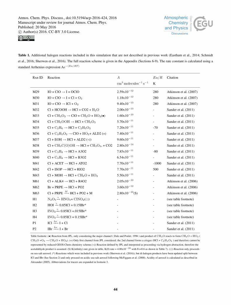
a range of updates beyond these. Updated or new reactions not included in Sherwen et al. (2016), Schmidt et al. (2016), or

Eastham et al. (2014) are given in Table 1 with a full description of the halogen chemistry scheme used given in Appendix25

Tables 6-9.

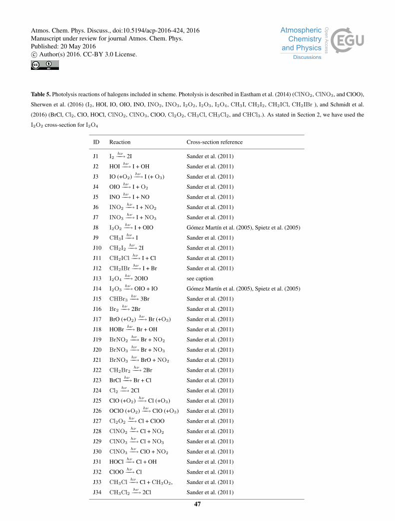
For the photolysis of I2OX (X=2,3,4) we have adopted the absorption cross-sections reported by Gómez Martín et al. (2005)

and Spietz et al. (2005) and used the I2O2 cross-section for I2O4. A quantum yield of unity was assumed for all I2OX species.

It is noted that recent work has used an unpublished spectrum for I2O4 that is much lower that I2O3 Saiz-Lopez et al. (2014),

but this is not expected to have a large effect on conclusions presented here.30

The parameterisation for oceanic iodide concentration was changed from Chance et al. (2014) to MacDonald et al. (2014)

as the latter resulted in an improved comparison with observations (see Section 7.5 of Sherwen et al. 2016).

3


The product of acid catalysed di-halogen release following I+ (HOI, INO2, INO3) uptake was updated from I2 as Sherwen

et al. (2016) to yield IBr and ICl following McFiggans et al. (2002). Acidity is calculated online through titration of sea salt

aerosol by uptake of sulfate dioxide (SO2), nitric acid (HNO3) and sulfuric acid (H2SO4) as described by Alexander (2005).

Re-release of IX (X=Cl,Br) is only permitted to proceed if the sea salt is acidic (Alexander, 2005). Thus aerosol cycling of

IX in the model is not a net source of IY (and may be a net sink on non-acid aerosol) but alters the speciation (Sherwen et al.,5

2016). The ratio between IBr and ICl was set to be 0.15:0.85 (IBr:ICl), instead of the 0.5:0.5 used previously (Saiz-Lopez

et al., 2014; McFiggans et al., 2000). A ratio of 0.5:0.5 gives a large overestimate of BrO with respect to the observations used

in Section 3.4.2 (Read et al., 2008; Volkamer et al., 2015). We attributed this reduction to the de-bromination of sea-salt which

we do not consider here, and the potential for the model to over estimate the BrOx lifetime. This is discussed further in the next

section but future laboratory and field studies of these heterogenous process are needed to help constrain these parameters.10

Iodine on aerosol is represented in the model with separate tracers based on the aerosol on which irreversible uptake occurs

(see Table 8). We include 3 iodine aerosol tracers to represent iodine on accumulation and coarse mode sea-salt and on sulfate

aerosol. The physical properties of the iodine aerosol tracers are assumed to be the same as its parent aerosol as previously

described for sulfate (Alexander et al., 2012) and sea-salt aerosol (Jaeglé et al., 2011).

We have added to the chlorine chemistry scheme described by Eastham et al. (2014) to include more tropospheric relevant15

reactions based on the JPL 10-6 compilation (Sander et al., 2011) and IUPAC (Atkinson et al., 2006). The heterogenous reaction

of N2O5 on aerosols was updated to yield products of ClNO2 and HNO3 (Bertram and Thornton, 2009; Roberts et al., 2009)

on sea salt, and 2HNO3 on other aerosol types. Reaction probabilities are unchanged (Evans and Jacob, 2005).

Deposition and photolysis of inter-halogen species (ICI, BrCl, IBr) and the reaction between ClO and IO were also included

(Sander et al., 2011).20

3 Model results

We run the model for two years (1/1/2004 to 1/1/2006), discarding the first year as a “spin-up” period and using the second year

(2005) for analysis. Non-halogen emissions are described in Sherwen et al. (2016). A reference simulation without any halogens

(“NOHAL”) was also performed. Where comparisons with observations are shown, the model is run for the appropriate year

with a 3 months “spin-up” before the observational dates, unless explicitly stated otherwise. The appropriate month from the25

2005 simulation is used as the initialisation for these observational comparisons to account for inter-annual variations. The

model is sampled at the nearest timestamp and grid box. The model only calculates chemistry in the troposphere. To avoid

confusion we do not show results above the tropopause (lapse rate of temperature falls below 2 K/km).

3.1 Emissions

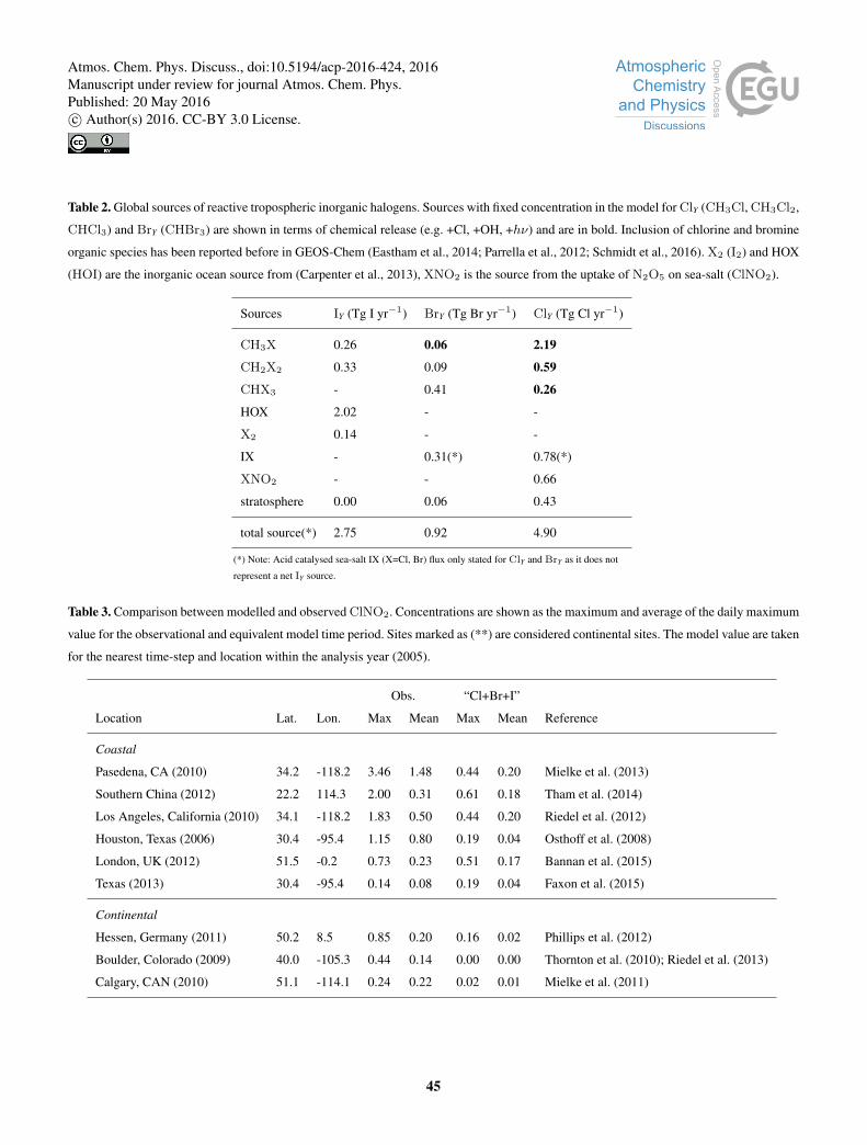
The emissions fluxes of chlorine, bromine, and iodine species are shown in Figure 1 with global totals in Table 2. We do not30

consider the Cl and Br contained within sea-salt as emitted in our simulation, following Schmidt et al. (2016) until a chemical

4


process liberates them into the gas-phase. These processes are the uptake of N2O5 on sea-salt and uptake of I+ species on

sea-salt. We do not include explicit sea-salt de-bromination for reasons described in Schmidt et al. (2016).

The organic iodine (CH3I, CH2I2, CH2ICl, CH2IBr) emissions are from Ordóñez et al. (2012) as described in Sherwen

et al. (2016). Inorganic iodine emissions (HOI, I2) (Carpenter et al., 2013; MacDonald et al., 2014) are 28 % lower here than

reported by Sherwen et al. (2016), due to use of the MacDonald et al. (2014) parameterisation for ocean surface iodide rather5

than that of Chance et al. (2014). Heterogeneous iodine aerosol chemistry (Section 2 and Appendix Section B1) does not lead

to a net release of iodine, instead just recycling it from less active forms (INO2, INO3, HOI) into more active forms (ICl/IBr).

The organic bromine (CH3Br, CHBr3, CH2Br2) emissions have been reported previously (Parrella et al., 2012; Schmidt

et al., 2016) and our simulation is consistent with this work. A further source of 0.031 Tg Br yr−1 (3.4 % of total) is included

here from CH2IBr photolysis. The heterogeneous cycling for BrY (defined in footnote below1) has been updated here from10

Schmidt et al. (2016), as described in Section 2/Appendix B1. An additional BrY source not considered by Schmidt et al.

(2016) is iodine activated IBr release from sea salt, which amounts to 0.31 Tg Br yr−1 and the majority (67 %) of this is

tropical (22◦N-22◦S). With all these updates, the tropospheric mean daytime (07:00-19:00) BrO concentration is 1.1 pmol

mol−1 (0.64 pmol mol−1 24 hr average), which is 13 % higher than reported in Schmidt et al. (2016).

The organic chlorine emission (CH3Cl, CHCl3, CH2Cl2) for this simulation (Table 2) has been described previously15

Schmidt et al. (2016) and set using fixed surface concentrations. An additional source of 0.046 Tg Cl yr−1(0.94 % of to-

tal) is present from CH2ICl photolysis (Sherwen et al., 2016). ClNO2 production from the heterogeneous uptake of N2O5

provides a source of 0.66 Tg Cl yr−1 (14 % of total) with the vast majority (95 %) being in the northern hemisphere, with

strongest sources in coastal regions north of 20oN. For June we calculate a global source of 21 Gg Cl month−1 which is

substantially less than the 62 Gg Cl month−1 (Pers. com. Sarwar Golam 2016) calculated in a previous study (Sarwar et al.,20

2014). The difference in NOX concentrations due to differences in model resolution probably contributes to this. Uptake of

HOI, INO2 and INO3 to sea-salt aerosol leads to the emission of ICl, giving an additional source of 0.78 Tg Cl yr−1 (17.6 %

of total) mostly (67 %) in tropical (22◦N-22◦S) locations.

Most of the emissions of Br and I species in our simulation occur in the tropics. It is notable that the chlorine emissions are

more widely distributed. This is as a result of longer lifetimes of chlorine precursor gases which moves their destruction further25

from their emissions and that the ClNO2 source is primarily in the northern extra tropics.

3.2 Deposition of halogens

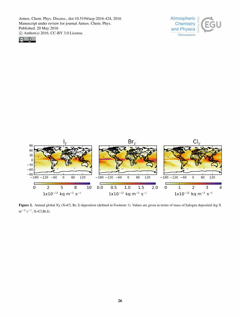
Figure 2 shows the global annual integrated wet and dry deposition of inorganic XY (X=Cl, Br,I). Much of the deposition of the

halogens occurs over the oceans (69 %, 83 %, and 90 % for ClY, BrY and IY respectively). It is high over regions of significant

tropical precipitation (ITCZ, Maritime continents, Indian Ocean) and much lower at the poles reflecting lower precipitation30

and emissions.

We find that the the major ClY depositional sink is HCl (85 %), with HOCl contributing 11 % and ClNO3 3.2 %. The BrY

sink is split between HBr, HOBr and BrNO3 with fractional contributions of 38, 30 and 24 % respectively. The major IY sink

1Here XY (X=Cl,Br,I) is the sum of gas-phase inorganic species of a given halogen in units of that halogen

5


is HOI deposition which represents 59 % of the depositional flux. The two next largest sinks are deposition of INO3 and iodine

aerosol (22 % and 15 %).

3.3 Halogen species concentrations

Figure 3 shows the surface and zonal concentration of annual mean IY, BrY, ClY, with Figure 4 showing the same for IO, BrO

and Cl, key halogen compounds in the atmosphere. Figure 5 showing the global molecule weighted mean vertical profile of the5

halogen speciation.

Inorganic iodine concentrations are highest in the tropical marine boundary layer consistent with their dominant emissions

regions. The highest concentrations are calculated in the coastal tropical regions, where enhanced O3 concentrations from in-

dustrial areas flow over high predicted oceanic iodide concentrations and lead to increased oceanic inorganic iodine emissions.

Within the vertical there is an average of ∼0.5-1 pmol mol−1 of IY consistent with previous model studies (Saiz-Lopez et al.,10

2014; Sherwen et al., 2016). The lowest concentrations of IY are seen just above the marine boundary layer where IY loss via

wet deposition is most favourable due to partitioning towards water soluble HOI. At higher altitudes, lower temperature and

high photolysis rates push the IY speciation to less water soluble compounds (IO, INO3) and hence the IY lifetime is longer. IO

concentrations (Figure 4) follow the concentrations of Iy with high concentrations in the tropical marine boundary layer. The

IO concentration increases into the upper troposphere reflecting a partitioning of Iy in this region towards IO (and IONO2) and15

away from HOI. The global mean tropospheric lifetimes of IY and IOX are 2.3 days and 1.3 minutes, respectively.

Total reactive bromine is more equally spread through the atmosphere than iodine. This reflects the longer lifetime of source

species with respect to photolysis which gives a more significant source higher in the atmosphere. The highest concentrations

are still found in the tropics. Unlike IY, BrY increases significantly with altitude, with BrNO3 and HOBr being the two most

dominant species. BrO concentrations (Figure 4) follows the concentration of inorganic bromine. In the boundary layer the20

highest concentrations are found in the tropical marine boundary layer concentrations are in the tropical marine boundary. BrO

and IO do not strongly correlate in the tropical marine boundary layer reflecting their differing sources. BrO concentrations

increase towards the upper troposphere associated with the increase in total Bry . The global annual average (molecule weighted)

tropospheric BrO mixing ratio in our simulation is 0.64 pmol mol−1 (Bry=4.5 pmol mol−1). When previous implementations

(Parrella et al., 2012; Schmidt et al., 2016) are run for the same year and model version as this work (GEOS-Chem v10), the25

modelled BrO concentrations are found to be 12 % lower than Schmidt et al. (2016), but 17 % higher than Parrella et al. (2012).

We calculate a tropospheric lifetime of BrY of 17 days and a BrOX lifetime of 15 minutes.

Total inorganic chlorine has a highly non-uniform distribution at the surface reflecting the dominance of the ClNO2 source

from N2O5 uptake on sea-salt. At the surface ClNO2, HCl, BrCl and HOCl represent around 25 % of the total ClY each. Away

from the surface the ClNO2 concentrations drop off rapidly due to the short lifetime of sea salt. HCl concentrations increase30

significantly into the middle and upper troposphere and dominate the ClY distribution. This suggests that stratospheric chlorine

freed from CFCs and organic chlorine strongly contributes to free tropospheric concentrations of ClY. However modelled ClY

is likely a lower limit on the concentrations in the uppermost troposphere (Froidevaux et al., 2008). Cl mixing ratios are very

low 0.075 fmol mol−1 or 2000 cm−3 in the marine boundary layer. Reactive Cl (ie not HCl) drop from the surface to around

6


10km where it then increases again towards to stratosphere. Cl shows a wider distrbution than IO and BrO reflecting the source

wider distribution of Cly . We calculate a tropospheric lifetime of ClY of 15 days, a ClOX lifetime of 2 seconds, and a global

tropospheric mean inorganic chlorine (ClY) concentration of 70 pmol mol−1 in our simulation.

The chemistry of halogens and sea-salt is highly uncertain (Simpson et al., 2015; Saiz-Lopez et al., 2012b; Abbatt et al.,

2012). Estimates for sea-salt de-bromination range from 0.51 Tg yr−1 (Parrella et al. 2012 implemented in GEOS-Chem v105

and v9-2) to 2.9 Tg yr−1 (Fernandez et al., 2014). Some studies have also not included sea-salt de-bromination (von Glasow

et al., 2004; Schmidt et al., 2016) as we do not in this work. Arguably this work therefore provides a lower estimate of bromine

and chlorine sources in the troposphere.

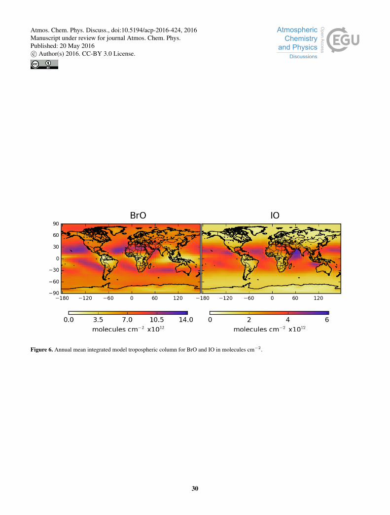
Figure 6 shows column integrated BrO and IO, which are the major halogen species for which we have observations (see

Section 3.4). Tropospheric ClO concentrations within the troposphere are small (see Figure 5) and are therefore not shown10

in Fig 6. Tropical maxima are seen for both BrO and IO, with BrO concentrations decreasing towards the equator. For IO a

localised maximum is seen in the Arabian Sea. The IO maximum in Antarctica reported from satellite retrievals (Schönhardt

et al., 2008) is not reproduced in our model potentially reflecting the lack of polar specific processes in the model.

3.4 Comparison with halogen observations

The observational dataset of tropospheric halogen compounds is sparse. Previous studies that this work is based on have shown15

comparisons for the oceanic precursors for chlorine (Eastham et al., 2014; Schmidt et al., 2016), bromine (Parrella et al., 2012;

Schmidt et al., 2016), and iodine (Bell et al., 2002; Sherwen et al., 2016; Ordóñez et al., 2012). The model performance in

simulating these compounds has not changed since these previous publications so we focus here on the available observations

of concentrations of IO, BrO, and some inorganic chlorine species (ClNO3, HCl and Cl2).

3.4.1 Iodine monoxide (IO)20

A comparison of IO to a suite of recent remote surface observations is shown in Fig 7. The model shows an overall negative

bias of 21 %. This compares with the 90 % positive bias previously reported in (Sherwen et al., 2016). This reduction in bias

is due to the use of the MacDonald et al. (2014) iodide parameterisation over that of Chance et al. (2014) which has reduced

the inorganic emission of iodine, along with the restriction of iodine recycling to acidic aerosol.

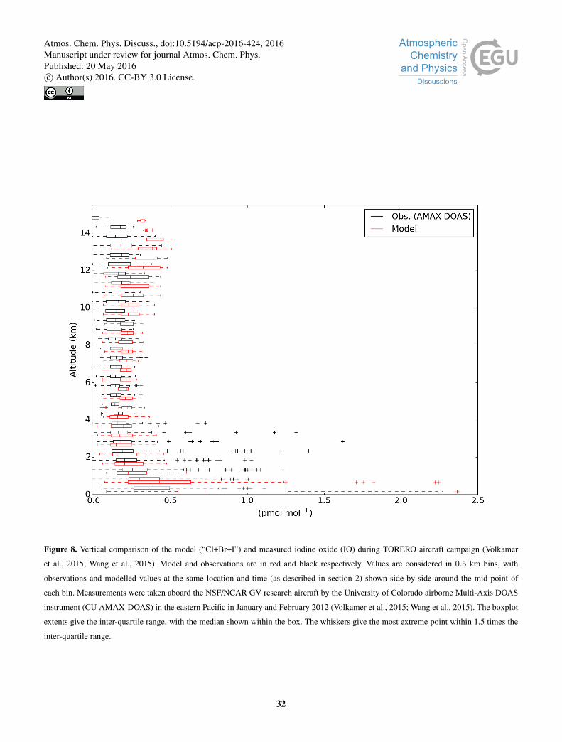
Figure 8 shows a comparison between modelled IO with altitude against observations in the eastern Pacific (Volkamer et al.,25

2015; Wang et al., 2015). In general, the model agreement with observations is good. There is an average bias of +40 % in

the free troposphere (350 hPa<p< 900 hPa), which increases to +58 % in the upper troposphere (350 hPa>p> tropopause).

As with the surface measurements, the model bias when comparing to IO observations (Volkamer et al., 2015; Wang et al.,

2015) in the free and upper troposphere is decreased from previously reported positive biases of 73 % and 96 %, respectively

(Sherwen et al., 2016).30

7


3.4.2 Bromine monoxide (BrO)

Comparisons of BrO against seasonal satellite tropospheric BrO observations from GOME-2 (Theys et al., 2011) are shown

in Figure 9. As shown previously (Parrella et al., 2012; Schmidt et al., 2016) the model has some skill in capturing both

the latitudinal and monthly variations in tropospheric BrO columns. However it underestimates the column BrO in the lower

southern latitudes (60◦S-90◦S), and to a smaller degree also in lower northern latitudes (60◦N-90◦N) which may reflect the5

lack of bromine from polar (blown snow, frost flowers etc.) sources and sea-salt de-bromination processes.

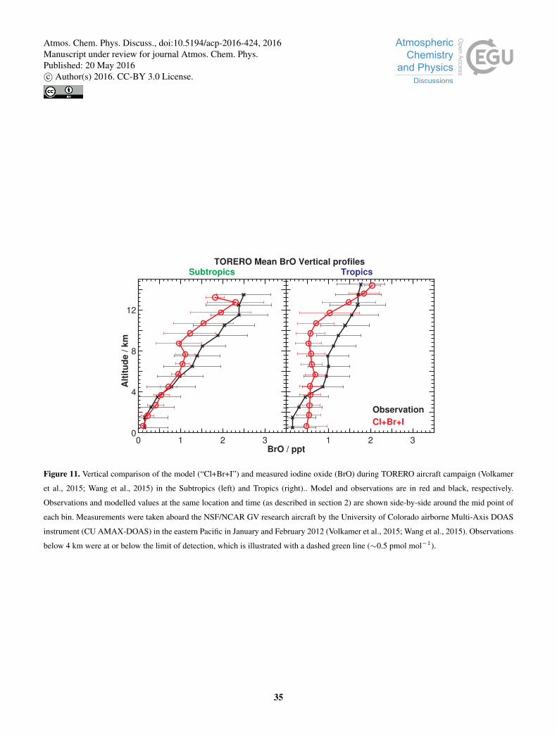
Figure 11 shows modelled vertical BrO concentrations against observations in the eastern Pacific (Volkamer et al., 2015;

Wang et al., 2015). We find a reasonable agreement within the free troposphere (350 hPa<p< 900 hPa) in both the tropics

and subtropics, with an average negative bias of 15 and 34 %, respectively. A similar comparisons is seen in the upper tropo-

sphere (350 hPa>p> tropopause) show similar negative biases for the tropics and subtropics, of 20 and 24 %, respectively.10

The decrease in agreement seen in the TORERO comparison (Fig. 11) relative to that previously presented in Schmidt et al.

(2016) is due to reduced BrCl and BrO production from slower cloud multiphase chemistry (see Sections B1-B3). We model

hihjer BrO concentrations in the tropical marine boundary layer above those observed (Volkamer et al., 2015). Our modelled

concentrations are lower than those reported previously (Miyazaki et al., 2016; Long et al., 2014; Pszenny et al., 2004; Keene

et al., 2009).15

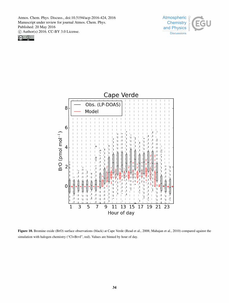
As shown in Fig. 10, comparisons between the model and observations of BrO made at Cape Verde (Read et al., 2008;

Mahajan et al., 2010) show a negative bias of 50 %. We attribute this to the high local sea-salt loadings at this site (Carpenter

et al., 2010), which is situated in the surf zone. This may locally increase the BrO concentrations. The model concentrations of

∼1 pmol mol−1 are however consistent with other ship borne observations made in the region (Leser et al., 2003).

Our model does not include sea-salt de-bromination and yet calculated roughly the correct concentrations of BrO. Inclu-20

sion of sea-salt de-bromination leads to excessively high BrO concentration in the model (Schmidt et al., 2016). Sea-salt

de-bromination is well observed, thus the success of the model despite the lack of inclusion of this process suggest model

failure in other areas. The BrOX lifetime may be too long. This is dominate by the reaction between Br and organics to produce

HBr. Oceanic sources of VOCs such as acetaldehyde have been proposed (Millet et al., 2010; Volkamer et al., 2015) and a

significant increase in the concentration of these species would lead to lower BrOX concentrations. Alternatively, a reduction25

in the efficiency of cycling of BrY through aerosol would also have a similar effect. The aerosol phase chemistry is complex

and the parameterisations used here may be too simple or fail to capture key processes (e.g. pH, organics). These all require

further study in order to help reconcile the rapidly growing body of observation of both gas and aerosol phase bromine in the

atmosphere with models.

3.4.3 Nitryl chloride (ClNO2), hydrochloric acid (HCl), hypochlorous acid (HOCl) and molecular chlorine (Cl2)30

Very few constraints on the concentration of tropospheric chlorine species are available.

An increasing number of ClNO2 observations are available (Table 3). We find that the model does reasonably well in coastal

regions, but does not reproduce observations in continental regions or regions with very high NOX.

8


Lawler et al. (2011) reports measurements of HOCl and Cl2 at Cape Verde for a week in June 2009. For the first 4 days

of the campaign, HOCl concentrations were higher and peaked at ∼100 pmol mol−1 with Cl2 concentrations peaking at ∼30

pmol mol−1. For the later days, HOCl concentrations dropped to around 20 pmol mol−1 and Cl2 concentrations to ∼0-10

pmol mol−1. We calculate much lower concentrations of Cl2 ( 1x10−3 pmol mol−1) and slightly lower HOCl ( 10 pmol

mol−1) throughout the same days of the year in our analysis year (2005). This is similar to findings of Long et al. (2014), who5

also found better comparisons with the cleaner period of observations. Similar to the comparison with observed ClNO2, our

simulation underestimates HOCl and Cl2.

The model does not include many sources of reactive chlorine. The failure to reproduce continental ClNO2 is likely due

to a lack of representation of sources such as salt plains, direct emission from power station and swimming pools, and HCl

acid displacement. The inability to reproduce the very high ClNO2 found in cities (Pasadena) and industrialised regions(Texas)10

may be due to the coarse resolution of the model compared to the spatial inhomogeneity of these observations. The failure to

reproduce the Cape Verde observations may be due to the very simple aerosol phase chlorine chemistry included in the model.

Overall we suggest that the model provides a lower limit estimate of the chlorine emissions and therefore burdens within the

troposphere, but constraints at the surface concentrations are limited and vertical profiles are not available. Further laboratory

work to better define aerosol processes and observations will be necessary to investigate the role of chlorine on tropospheric15

chemistry.

4 Impact of halogens

We now investigate the impact of the halogen chemistry on the composition of the troposphere. We start with O3 and OH and

then move onto other components of the troposphere.

4.1 Ozone (O3)20

Figure 12 shows changes in column, surface and zonal O3 both in absolute and fractional terms between simulations with and

without halogen emissions (“Cl+Br+I” vs “NOHAL”). Globally the mass-weighted, annual-average mixing ratio is reduced by

7.4 pmol mol−1 (14.6%) with the inclusion of halogens (“Cl+Br+I”-“NOHAL”)/“NOHAL”*100). A much larger percentage

decrease of 25.0 % (7.2 pmol mol−1) is seen over the ocean surface. Large percentage losses are seen in the oceanic southern

hemisphere as reported previously (Long et al., 2014; Schmidt et al., 2016; Sherwen et al., 2016) reflecting the significant25

ocean-atmosphere exchange in this regions. The majority (65 %) of the change in O3 mass due to halogens occurs in the free

troposphere (350 hPa<p<900 hPa).

Comparisons of the model and observed surface and sonde O3 concentrations are given in Figures 13 and 14. In the tropics

the fidelity of the simulation improves with the inclusion of halogens (Schmidt et al., 2016; Sherwen et al., 2016). Sonde and

surface comparisons north of ∼50◦N and south of ∼60◦S however show that the model now underestimates O3.30

9


The global odd oxygen budget (OX, as defined in the footnote below2) in the troposphere with (“Cl+Br+I”) and without

halogens (“NOHAL”) is shown in Table 4. The OX loss through chlorine, bromine, and iodine represents 0.46, 5.8 and 12 %

of the total OX loss respectively, thus halogens constitute 18.2 % of the overall O3 loss. The sum of halogen driven OX loss is

900 Tg OX yr−1 , which is similar to the magnitude of loss via reaction of O3 with HO2 of ∼1100 Tg OX yr−1 (23 % of total).

Halogen cross-over reactions (BrO+IO, BrO+ClO, IO+ClO) contribute little to the overall O3 loss. This number compares with5

∼930 Tg OX yr−1 reported in GEOS-Chem previously by Sherwen et al. (2016). Saiz-Lopez et al. (2014) found that, between

50◦S-50◦N and over ocean only, halogens are responsible for the loss of 640 Tg OX yr−1. We find a comparable value of 670

OX yr−1 with our model.

The majority of the halogen driven O3 loss (58.1 %) occurs in the free troposphere (350 hPa<p<900 hPa). Halogens

represent 34.9 and 31.0 % of OX loss in the upper troposphere (350 hPa>p> tropopause) and marine boundary layer (90010

hPa<p ) respectively as shown in Figure 15. The marine boundary layer OX loss attributable to halogens is equal to the 31

% reported by Prados-Roman et al. (2015a) previously, and it is slightly higher than that reported solely for iodine of 26 %

(Sherwen et al., 2016).

Although the partitioning between the OX loss processes is significantly different between the simulations with halogens

and without (Table 4), the overall annual OX loss only increases by 2.2 % (4933 vs 4829 Tg yr−1). The OX production term15

decreases by 1.0 %. This decrease is due to a reduction in NOX concentrations due to hydrolysis of XNO3 (X=Cl, Br, I). Our

tropospheric NOX burden decreases by 1.7 % to 168 Gg N (see table 10) on inclusion of halogens consistent with observations

and previous model studies (Long et al., 2014; von Glasow et al., 2004; Parrella et al., 2012; Schmidt et al., 2016). Globally

NOX loss through ClNO3 and BrNO3 hydrolysis is approximately equal (1:0.86), and overall proceeds at a rate of ∼10 %

of the NOX loss through the NO2+OH pathway. Iodine nitrite and nitrate (INO2, INO3) hydrolysis is much less significant20

(∼0.25 % of rate of NO2+OH). Net OX is the difference between the production and loss terms and the change here is much

greater leading to an overall decrease in net production of tropospheric O3 (POX-LOX) of 26 % (159 Tg yr−1), and a resultant

in decrease O3 lifetime of 14 %.

4.2 HOX (OH+HO2)

We find that global molecule weighted average HOX (OH+HO2) concentrations are reduced by 8.5 % with the inclusion of25

halogens, with OH decreasing by 4.5 % from 1.40x106 to 1.34x106 molecules cm−3. Lower O3 concentrations decrease the

primary OH source (O3hν−→2OH) by 15.5 %, and the secondary OH source from HO2+NO by 2.2 %.

The reduction in the sources of OH is buffered by an additional OH source from the photolysis of HOX (X=Cl, Br, I) which

acts to increase the conversion of HO2 to OH. Previously, Sherwen et al. (2016) showed an increase of 1.8 % in global OH

concentrations on inclusion of iodine. However, increased BrY and reduced IY concentrations in the simulations described here30

mean that the increased OH source from HOX photolysis does not compensate fully for the reduced primary source, resulting

2Here OX is defined as O3 +NO2 +2NO3 +PAN+PMN+PPN+HNO4 +3N2O5 +HNO3 +MPN+XO+HOX+XNO2 +2XNO3 +

2OIO+2I2O2 +3I2O3 +4I2O4 +2Cl2O2 +2OClO, where X=Cl, Br, I; PAN = peroxyacetyl nitrate; PPN = peroxypropionyl nitrate; MPN = methyl

peroxy nitrate; and PMN = peroxymethacryloyl nitrate.

10


in an overall 4.5 % reduction in global mean OH. This buffering contributes to a smaller change in OH than report previously

by Schmidt et al. (2016) of 11 %. As reported previously (Long et al., 2014; Schmidt et al., 2016), we also find the net effect

of halogens on the OH:HO2 ratio is a small increase (4.4 %).

4.3 Organic Compounds

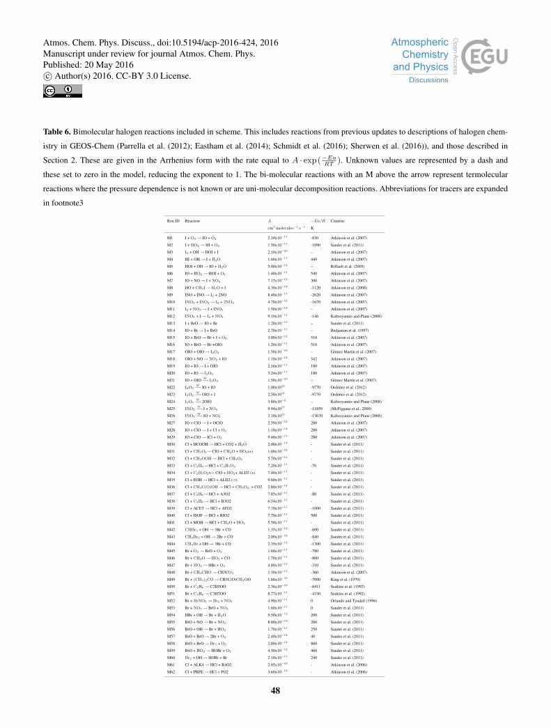
The oxidation of volatile organic compounds (VOCs) by halogens is included in this simulation (see Table 6 for reactions).5

The global fractional loss due to OH, Cl, Br, NO3, and photolysis for a range of organics is shown in Figure 16.

Globally, Br oxidation is small in our simulation and contributes 2.0 % to the loss of acetaldehyde (CH3CHO), 0.6 %

of the loss of formaldehyde (CH2O), 0.26 % of the loss of >C4 alkenes, and < 0.001 % of the loss of other compounds.

Recent work has suggests a significant source of oceanic oxygenated VOCs (Millet et al., 2010; Coburn et al., 2014; Sinreich

et al., 2010; Mahajan et al., 2014; Lawson et al., 2015; Volkamer et al., 2015; Myriokefalitakis et al., 2008) which we do not10

include in this simulation. Furthermore although our modelled BrY is broadly comparable to some previous work (Schmidt

et al., 2016; Parrella et al., 2012), it is lower in the marine boundary layer than in other recent work (Long et al., 2014). The

combination of these two factors suggest that our model provides a lower bounds of impacts of bromine on VOCs. Significantly

higher concentrations of oVOC would decrease the BrO concentrations in the model and might then allow an increased sea-salt

source of reactive bromine.15

The oxidation of Volatile Organic Compounds (VOCs) by chlorine is more significant. In our simulation chlorine accounts

for 18, 9, and 9 % of the global loss of ethane (C2H6), propane (C3H8), and acetone (CH3C(O)CH3)), respectively. Loss

of other VOCs is globally small. This increased loss due to Cl is to some extent compensated for by the reduction in the OH

concentrations that we calculate. Thus the overall lifetime of ethane, propane, and acetone changes from 131, 38, 85 days in

the simulation without halogens to 120, 37, 82 in the simulation with halogens. Notably the ethane lifetime without halogens20

is 10% longer than it is with. Given that we consider the chlorine in the model to be a lower limit, ethane oxidation by chlorine

may in reality be more significant than found here.

Methane is a significant climate gas, as it has the second highest forcing amongst well-mixed greenhouse gases from prein-

dustrial to present day (Myhre et al., 2013). In our simulation without halogens we calculate a tropospheric chemical lifetime

due to OH of 7.48 years. With the inclusion of halogen chemistry the OH concentration drops, extending the methane lifetime25

due to OH of become to 7.96 years (an increase of 6.5 %). However, in our halogen simulations, chlorine radicals also oxidise

methane (∼1 % of the total loss) shortening the lifetime to 7.89 years (0.85 %). As noted previously, the model’s chlorine

concentrations appear to be underestimated. Allan et al. (2007) estimate a 25 Tg yr−1 sink for methane from Cl (∼4 %), sig-

nificantly higher than our estimate. Overall the model’s CH4 lifetime still appears to be short compared to the observationally

based estimation of 9.1 ± 0.9 from Prather et al. (2012), but halogens decrease this bias.30

In our simulations, halogens (essentially chlorine) have a significant but not overwhelming role in the concentrations of

hydrocarbons (from∼1 % of methane loss to∼18 % of ethane loss). However, as discussed earlier the low biases seen with the

very limited observational dataset of chlorine compounds would suggest that the impacts calculated here are probably lower

limits.

11


4.4 Other species

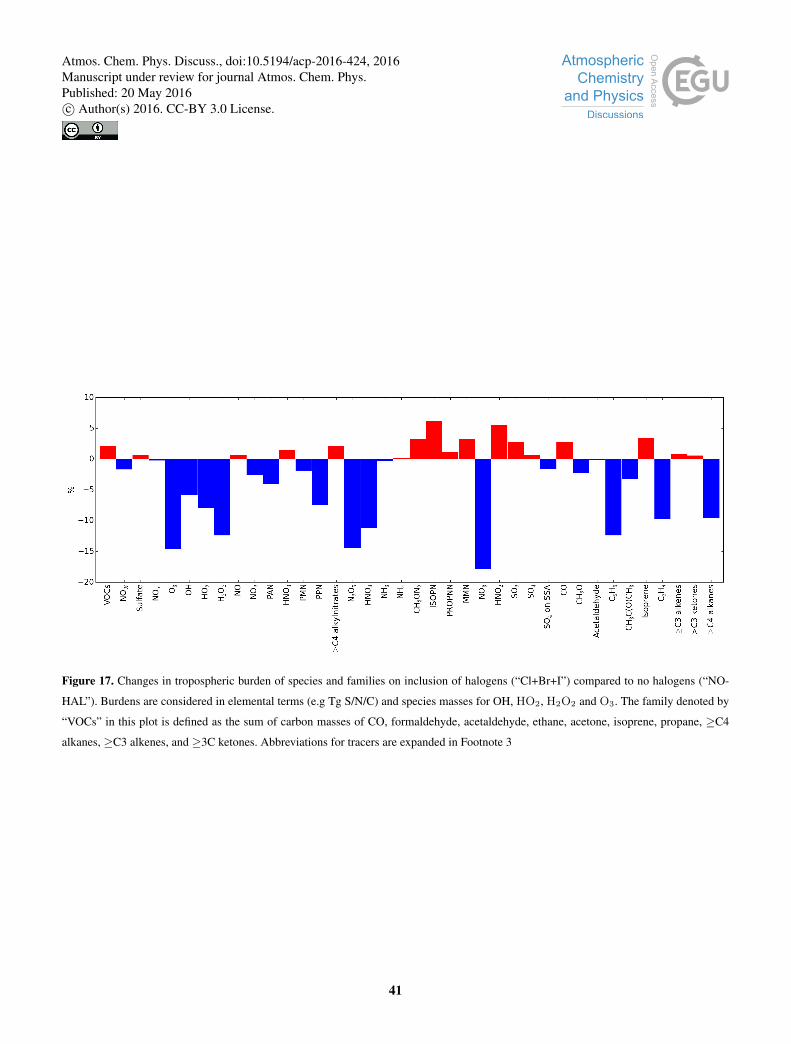
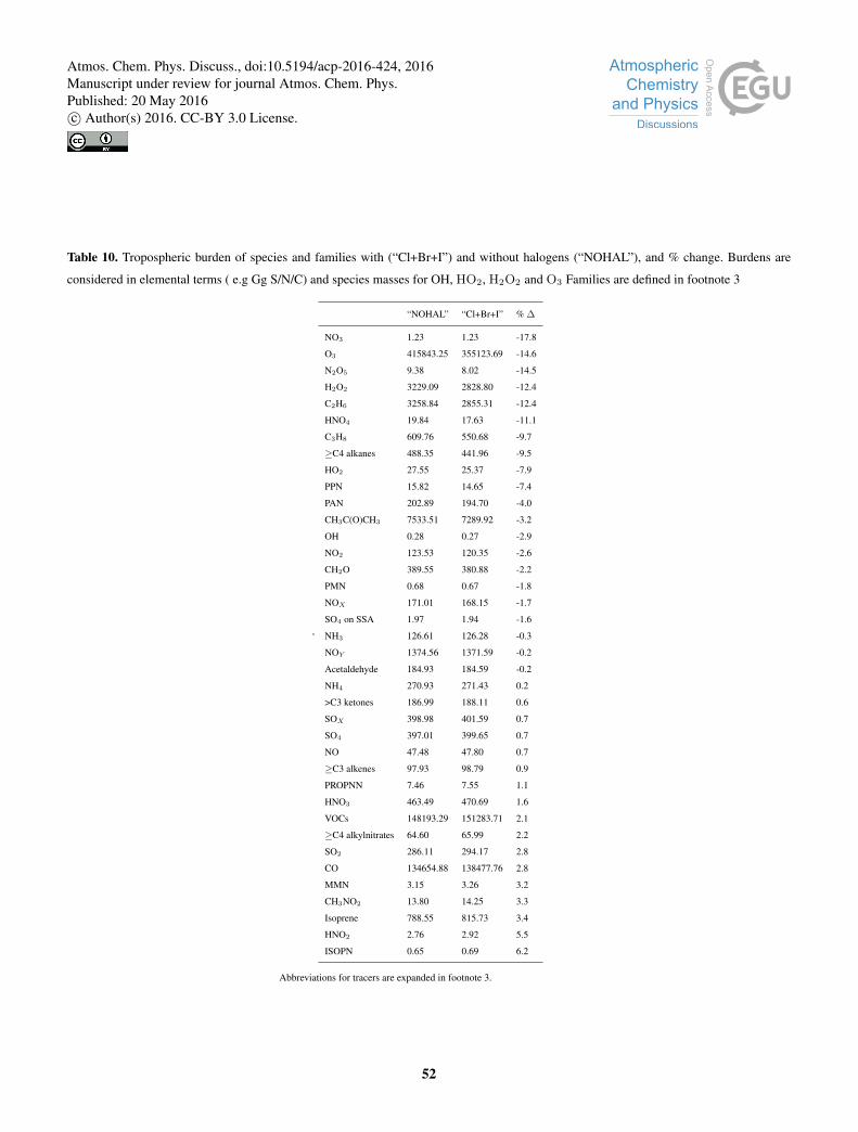
With the inclusion of halogens in the troposphere there are a large number of changes in the composition of the troposphere.

Figure 17 illustrates the fractional global change in burden by species (for abbreviation see footnote3). The spatial and zonal

distribution of these changes by species family (HOX, NOX, SOX as defined in footnote4) are shown in Figure 18 and for a few

VOCs (C3H8, C2H6, acetone, and >C4 alkanes) in Figure 19. A tabulated form of these changes is given within the Appendix5

(Table 10)

As discussed in section 4.1 and 4.1, a clear decrease in oxidants (O3, OH, HO2, H2O2) is seen. This drives an increase in

the concentrations of some VOCs (2.1 % on a per carbon basis), including CO (2.8 %) and Isoprene (3.4 %). However, as

discussed, it also adds an additional Cl sink term which leads to an overall decrease in some species (e.g. C2H6, (CH3)2CO,

C3H8) particularly in the northern hemisphere oceanic regions. The SOX burden increases slightly (0.7 %), which can be10

attributed to decreases in oxidants.

5 Summary and Conclusions

We have presented a model of tropospheric composition which has attempted to include the major routes of halogen chemistry

impacts. Assessment of the model performance is limited as observations of halogen species are extremely sparse. However,

given the available observations we conclude that the model has some useful skill in predicting the concentration of iodine and15

bromine species and appears to underestimate the concentrations of chlorine species.

Consistent with previous studies, our model shows significant halogen driven changes in the concentrations of oxidants.

The tropospheric O3 burden and global mean OH decreased by 14.6 %, and 4.5 % respectively, on inclusion of halogens. The

methane lifetime increases by 6.5 %, improving agreement with observations.

There are a range of changes in the concentrations of other species. Direct reaction with Cl atoms leads to enhanced oxida-20

tion of hydrocarbons with ethane showing a significant response. Given the model appears to provide a lower limit for atomic

Cl concentrations this suggests a major missing oxidation pathway for ethane which is currently not considered. NOX concen-

trations are reduced by aerosol hydrolysis of the halogen nitrates which leads to reduced global O3 production. Our simulation

of BrO appears to be relatively consistent with those observed, however we do not include sea-salt de-bromination mechanism.

This would suggest that either the cycling of bromine in our model is generally too fast, or that we do not have sufficiently25

large BrOX sinks (potentially oVOCs). Both hypothesis warrant further research.

Significant uncertainties however remain in our understanding of halogens in the troposphere. The gas phase chemistry and

photolysis parameters of iodine compounds are uncertain, together with the emissions of their organic and inorganic precursors

(Sherwen et al., 2016). For chlorine, bromine and iodine heterogeneous chemistry, little experimental data exists and suitable

3Abbreviated species names are defined in the GEOS-Chem manual (http://acmg.seas.harvard.edu/geos/doc/man/appendix_6.html) and here:

MOH=Methanol, EOH=Ethanol, ALD2=Acetaldehyde, ISOP=Isoprene, ALK4=≥C4 alkanes, CH3O2,=Methylperoxy radical, A3O2= primary RO2 from

C3H8, B3O2=secondary RO2 from C3H8, ATO2=RO2 from Acetone, R4O2=RO2 from ≥C4 alkanes, RIO2=RO2 from Acetone4 Here we define families of HOX, NOX and SOX as follows. HOX: OH + HO2, NOX: NO+NO2, SOX : SO2 + SO4 + SO4 on sea salt.

12


parameterisations for the complex aerosols found in the atmosphere are unavailable (Abbatt et al., 2012; Saiz-Lopez et al.,

2012b; Simpson et al., 2015).

Understanding fully the impact of halogens on tropospheric composition will require significant development of new experi-

mental techniques and more field observations, new laboratory studies and models which are able to exploit these developments.

Appendix A: Tabulated Burden Changes on inclusion of halogens5

Table 10 gives the burdens with and without halogens and the fractional change.

Appendix B: Gas phase Chemistry Scheme

Here is described the full halogen chemistry scheme as presented in previous work (Bell et al., 2002; Eastham et al., 2014;

Parrella et al., 2012; Schmidt et al., 2016; Sherwen et al., 2016) and with updates as detailed in section 2 and Table 1. The

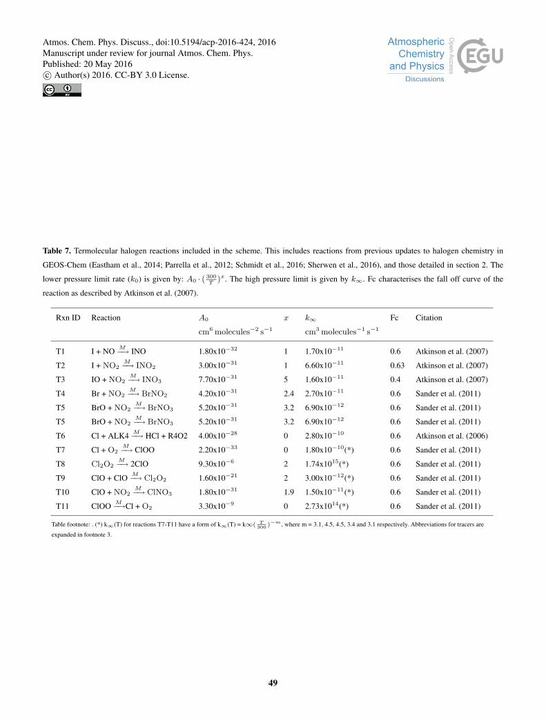
complete gas phase photolysis, bimolecular and termolecular reactions are described in Tables 5 ,6 and 7 .10

B1 Heterogenous reactions

The halogen multiphase chemistry mechanism is based on the iodine mechanism (“Br+I”) described in Sherwen et al. (2016)

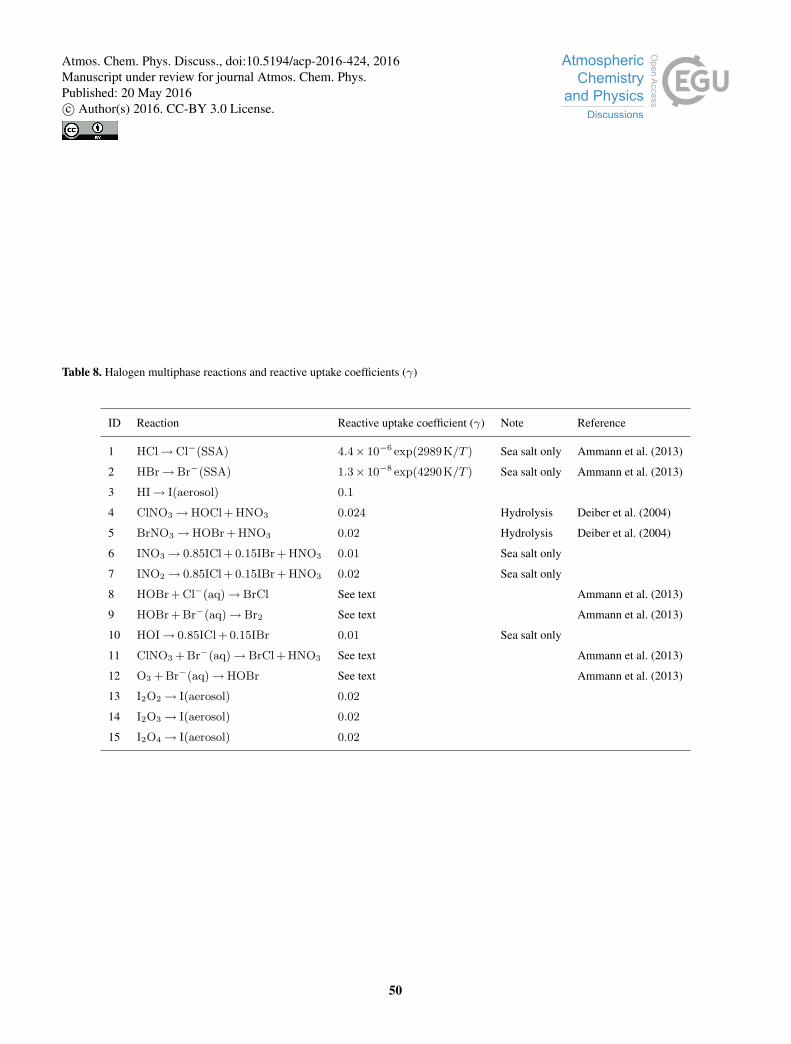
and the coupled mechanism of Schmidt et al. (2016). The heterogenous reactions in the scheme are shown in Table 8 and

with further detail individual detail on certain reactions below. The loss rate of a molecule X due to multiphase processing on

aerosol is calculated following Jacob (2000).15

dnXdt

=−(r

Dg+

4cγ

)−1

AnX , (B1)

where r is the aerosol effective radius, Dg is the gas phase diffusion coefficient of X, c is the average thermal velocity of X,

γ is the reactive uptake coefficient, A is the aerosol surface area concentration, and nX is the gas phase concentration of X.

B2 Aerosols

We consider halogen reactions on sulfate aerosols, sea salt aerosols, and liquid and ice cloud droplets. The implementation of20

sulfate type aerosols in GEOS-Chem is described by Park et al. (2004) and Pye et al. (2009). Sulfate aerosols are assumed to

be acidic with pH=0.

The GEOS-Chem sea salt aerosol simulation is as described by Jaeglé et al. (2011). The transport and deposition of sea

salt bromide follows that of the parent aerosol. Oxidation of bromide on sea-salt produces volatile forms of bromine that are

released to the gas phase. Sea salt aerosol is emitted alkaline, but the alkalinity can be titrated in GEOS-Chem by uptake of25

HNO3, SO2, H2SO4 (Alexander, 2005). Sea salt aerosol with no remaining alkalinity is assumed to have pH=5. We assume

no halide oxidation on alkaline sea salt aerosol.

13


The liquid cloud droplet surface area is modelled using cloud liquid water content from GEOS-FP (Lucchesi, 2013) and

assuming effective cloud droplet radii of 10 µm and 6 µm for marine and continental clouds, respectively. The ice cloud

droplet surface area is modelled in a similar manner assuming effective ice droplet radii of 75 µm. We assume that ice cloud

chemistry is confined to an unfrozen overlayer surrounding the ice crystal, see Schmidt et al. (2016) for details. Cloud water

pH (typically between 4 and 6) is calculated locally in GEOS-Chem following (Alexander et al., 2012).5

The reactive uptake coefficients depend on the aerosol halide concentration. For sea salt aerosol, the bromide concentration

is calculated directly from the bromide content and the aerosol mass. Sea salt aerosol chloride is assumed to be in excess (see

below). For clouds and sulfate aerosol, the bromide and chloride concentration is estimated assuming equilibrium between gas

phase HX and aerosol phase X−.

B3 Reactive uptake coefficients10

B3.1 HOBr +Cl−/Br−

The reactive uptake coefficient is calculated as

γ =(Γ−1 +α−1

)−1, (B2)

where the mass accomodation coefficient for HOBr is α= 0.6 and

Γ =4HHOBrRTkHOBr+X− [X−][H+]lrf(r, lr)

c, (B3)15

with kHOBr+Cl− = 5.9× 109 M−2s−1 and kHOBr+Br− = 1.6× 1010 M−2s−1. In the equation above c is the average thermal

velocity of HOBr, and f(lr, r) is a reacto-diffusive correction factor,

f(lr, r) = coth(r

lr

)− lrr, (B4)

with r being the radius of the aerosol. For sea salt aerosol HOBr + Cl− is assumed to be limited by mass accommodation, i.e.

Γ� α, due to high concentration of Cl− in sea salt aerosol. The reacto-diffusive length scale is20

lr =

√Dl

kHOBr+X− [X−][H+], (B5)

where Dl = 1.4× 10−5 cm2s−1 is the aqueous phase diffusion coefficient for HOBr. The listed parameters are taken from

Ammann et al. (2013), and kHOBr+Br− is from Beckwith et al. (1996).

B3.2 ClNO3 + Br−

The reactive uptake coefficient is calculated as25

γ =(Γ−1 +α−1

)−1, (B6)

14


where the mass accomodation coefficient for ClNO3 is α= 0.108 and

Γ =4WRT

√[Br−]Dl

c, (B7)

where c is the average thermal velocity of ClNO3, Dl = 5.0× 10−6 cm2s−1 is the aqueous phase diffusion coefficient for

ClNO3, and W = 106√

Ms bar−1.

B3.3 O3 + Br−5

The reactive uptake coefficient is calculated as

γ = Γb + Γs, (B8)

where Γb is the bulk reaction coefficient,

Γb =4HO3RTkO3+Br− [Br−]lrf(r, lr)

c, (B9)

with kO3+Br− = 6.8× 108 exp(−4450K/T )M−1s−1. In the equation above c is the average thermal velocity of O3, and10

f(lr, r) is a reacto-diffusive correction factor,

f(lr, r) = coth(r

lr

)− lrr, (B10)

with r being the radius of the aerosol. The reacto-diffusive length scale is

lr =

√Dl

kO3+Br− [Br−], (B11)

where Dl = 8.9× 10−6 cm2s−1 is the aqueous phase diffusion coefficient for O3.15

The surface reaction coefficient is calculated as,

Γs =4ks[Br−(surf)]KLangCNmax

c(1 +KLangC[O3(g)]), (B12)

where the surface reaction rate constant is ks = 10−16 cm2s−1, the equilibrium constant for O3 is KLangC = 10−13 cm3, and

the maximum number of available sites is taken as Nmax = 3×1014 cm−2. The surface bromide concentration is estimated as,

20

[Br−(surf)] = min(3.41× 1014 cm−2M−1 [Br−],Nmax). (B13)

Acknowledgements. This work was funded by NERC quota studentship NE/K500987/1 with support from the NERC BACCHUS and CAST

projects NE/L01291X/1, NE/J006165/1.

J. A. Schmidt acknowledges funding through a Carlsberg Foundation post-doctoral fellowship (CF14-0519)

R. Volkamer acknowledges funding from US National Science Foundation CAREER award ATM-0847793, AGS-1104104, and AGS-25

1452317. The involvement of the NSF-sponsored Lower Atmospheric Observing Facilities, managed and operated by the National Center

for Atmospheric Research (NCAR) Earth Observing Laboratory (EOL), is acknowledged.

T. Sherwen would like to acknowledge constructive comments and input from GEOS-Chem Support Team.

15


References

Abbatt, J. P. D., Lee, A. K. Y., and Thornton, J. A.: Quantifying trace gas uptake to tropospheric aerosol: recent advances and remaining

challenges, Chem. Soc. Rev., 41, 6555–6581, doi:10.1039/c2cs35052a, 2012.

Alexander, B.: Sulfate formation in sea-salt aerosols: Constraints from oxygen isotopes, J. Geophys. Res., 110, D10 307,

doi:10.1029/2004JD005659, 2005.5

Alexander, B., Allman, D. J., Amos, H. M., Fairlie, T. D., Dachs, J., Hegg, D. A., and Sletten, R. S.: Isotopic constraints on the formation

pathways of sulfate aerosol in the marine boundary layer of the subtropical northeast Atlantic Ocean, J. Geophys. Res., 117, D06 304,

doi:10.1029/2011JD016773, 2012.

Allan, W., Struthers, H., and Lowe, D. C.: Methane carbon isotope effects caused by atomic chlorine in the marine boundary layer: Global

model results compared with Southern Hemisphere measurements, J Geophys. Res-Atmos., 112, doi:10.1029/2006JD007369, 2007.10

Ammann, M., Cox, R. A., Crowley, J. N., Jenkin, M. E., Mellouki, A., Rossi, M. J., Troe, J., and Wallington, T. J.: Evaluated kinetic and

photochemical data for atmospheric chemistry: Volume VI – heterogeneous reactions with liquid substrates, Atmos. Chem. Phys., 13,

8045–8228, doi:10.5194/acp-13-8045-2013, 2013.

Atkinson, R., Baulch, D. L., Cox, R. A., Crowley, J. N., Hampson, R. F., Hynes, R. G., Jenkin, M. E., Rossi, M. J., Troe, J., and IUPAC

Subcommittee: Evaluated kinetic and photochemical data for atmospheric chemistry: Volume II – gas phase reactions of organic15

species, Atmos. Chem. Phys., 6, 3625–4055, doi:10.5194/acp-6-3625-2006, 2006.

Atkinson, R., Baulch, D. L., Cox, R. A., Crowley, J. N., Hampson, R. F., Hynes, R. G., Jenkin, M. E., Rossi, M. J., and Troe, J.: Evaluated

kinetic and photochemical data for atmospheric chemistry: Volume III - gas phase reactions of inorganic halogens, Atmos. Chem. Phys.,

7, 981–1191, 2007.

Atkinson, R., Baulch, D. L., Cox, R. A., Crowley, J. N., Hampson, R. F., Hynes, R. G., Jenkin, M. E., Rossi, M. J., Troe, J., and Wallington,20

T. J.: Evaluated kinetic and photochemical data for atmospheric chemistry: Volume IV - gas phase reactions of organic halogen species, J.

Phys. Chem. Ref. Data, 8, 4141–4496, 2008.

Bannan, T. J., Booth, A. M., Bacak, A., Muller, J. B. A., Leather, K. E., Le Breton, M., Jones, B., Young, D., Coe, H., Allan, J., Visser,

S., Slowik, J. G., Furger, M., Prévôt, A. S. H., Lee, J., Dunmore, R. E., Hopkins, J. R., Hamilton, J. F., Lewis, A. C., Whalley, L. K.,

Sharp, T., Stone, D., Heard, D. E., Fleming, Z. L., Leigh, R., Shallcross, D. E., and Percival, C. J.: The first UK measurements of nitryl25

chloride using a chemical ionization mass spectrometer in central London in the summer of 2012, and an investigation of the role of Cl

atom oxidation, J Geophys. Res-Atmos., 120, 5638–5657, doi:10.1002/2014JD022629, 2015.

Beckwith, R. C., Wang, T. X., and Margerum, D. W.: Equilibrium and Kinetics of Bromine Hydrolysis, Inorg. Chem., 35, 995–1000,

doi:10.1021/ic950909w, 1996.

Bedjanian, Y., Le Bras, G., and Poulet, G.: Kinetic study of the Br + IO, I + BrO and Br + I2 reactions. Heat of formation of the BrO radical,30

Chem. Phys. lett., 266, 233–238, doi:http://dx.doi.org/10.1016/S0009-2614(97)01530-3, 1997.

Bell, N., Hsu, L., Jacob, D. J., Schultz, M. G., Blake, D. R., Butler, J. H., King, D. B., Lobert, J. M., and Maier-Reimer, E.: Methyl iodide:

Atmospheric budget and use as a tracer of marine convection in global models, J. Geophys. Res-Atmos., 107, ACH 8–1–ACH 8–12,

doi:10.1029/2001jd001151, 2002.

Bertram, T. H. and Thornton, J. A.: Toward a general parameterization of N2O5 reactivity on aqueous particles: the competing effects of35

particle liquid water, nitrate and chloride, Atmos. Chem. Phys., 9, 8351–8363, doi:10.5194/acp-9-8351-2009, 2009.

16


Bloss, W. J., Evans, M. J., Lee, J. D., Sommariva, R., Heard, D. E., and Pilling, M. J.: The oxidative capacity of the troposphere: Coupling

of field measurements of OH and a global chemistry transport model, Faraday Discuss., 130, 425–436, doi:10.1039/b419090d, 2005.

Carpenter, L. J., Fleming, Z. L., Read, K. A., Lee, J. D., Moller, S. J., Hopkins, J. R., Purvis, R. M., Lewis, A. C., Muller, K., Heinold, B.,

Herrmann, H., Fomba, K. W., van Pinxteren, D., Muller, C., Tegen, I., Wiedensohler, A., Muller, T., Niedermeier, N., Achterberg, E. P.,

Patey, M. D., Kozlova, E. A., Heimann, M., Heard, D. E., Plane, J. M. C., Mahajan, A., Oetjen, H., Ingham, T., Stone, D., Whalley, L. K.,5

Evans, M. J., Pilling, M. J., Leigh, R. J., Monks, P. S., Karunaharan, A., Vaughan, S., Arnold, S. R., Tschritter, J., Pohler, D., Friess,

U., Holla, R., Mendes, L. M., Lopez, H., Faria, B., Manning, A. J., and Wallace, D. W. R.: Seasonal characteristics of tropical marine

boundary layer air measured at the Cape Verde Atmospheric Observatory, J. Atmos. Chem., 67, 87–140, doi:10.1007/s10874-011-9206-1,

2010.

Carpenter, L. J., MacDonald, S. M., Shaw, M. D., Kumar, R., Saunders, R. W., Parthipan, R., Wilson, J., and Plane, J. M. C.: Atmospheric10

iodine levels influenced by sea surface emissions of inorganic iodine, Nature Geosci., 6, 108–111, doi:10.1038/ngeo1687, 2013.

Chameides, W. L. and Davis, D. D.: Iodine: Its possible role in tropospheric photochemistry, J Geophys. Res-Oceans, 85, 7383–7398,

doi:10.1029/JC085iC12p07383, 1980.

Chance, R., Baker, A. R., Carpenter, L., and Jickells, T. D.: The distribution of iodide at the sea surface, Environ. Sci.: Processes Impacts,

16, 1841–1859, doi:10.1039/C4EM00139G, 2014.15

Coburn, S., Ortega, I., Thalman, R., Blomquist, B., Fairall, C. W., and Volkamer, R.: Measurements of diurnal variations and eddy co-

variance (EC) fluxes of glyoxal in the tropical marine boundary layer: description of the Fast LED-CE-DOAS instrument, Atmospheric

Measurement Techniques, 7, 3579–3595, doi:10.5194/amt-7-3579-2014, 2014.

Coburn, S., Dix, B., Edgerton, E., Holmes, C. D., Kinnison, D., Liang, Q., ter Schure, A., Wang, S., and Volkamer, R.: Mercury oxidation

from bromine chemistry in the free troposphere over the Southeastern US, Atmos. Chem. Phys., 16, 3363–3378, doi:doi:10.5194/acp-16-20

3743-2016, 2016.

Dean, J. A.: Lange’s Handbook of Chemistry, McGraw-Hill, Inc., 1992.

Deiber, G., George, C., Le Calvé, S., Schweitzer, F., and Mirabel, P.: Uptake study of ClONO2 and BrONO2 by Halide containing droplets,

Atmos. Chem. Phys., 4, 1291–1299, doi:10.5194/acp-4-1291-2004, 2004.

Eastham, S. D., Weisenstein, D. K., and Barrett, S. R. H.: Development and evaluation of the unified tropospheric–stratospheric25

chemistry extension (UCX) for the global chemistry-transport model GEOS-Chem, Atmos. Environ., 89, 52–63,

doi:http://dx.doi.org/10.1016/j.atmosenv.2014.02.001, 2014.

Evans, M. J. and Jacob, D. J.: Impact of new laboratory studies of N2O5 hydrolysis on global model budgets of tropospheric nitrogen oxides,

ozone, and OH, Geophys. Res. Lett., 32, L09 813, doi:10.1029/2005GL022469, 2005.

Faxon, C. B., Bean, J. K., and Ruiz, L. H.: Inland Concentrations of Cl2 and ClNO2 in Southeast Texas Suggest Chlorine Chemistry30

Significantly Contributes to Atmospheric Reactivity, Atmosphere, 6, 1487, doi:10.3390/atmos6101487, 2015.

Fernandez, R. P., Salawitch, R. J., Kinnison, D. E., Lamarque, J.-F., and Saiz-Lopez, A.: Bromine partitioning in the tropical tropopause

layer: implications for stratospheric injection, Atmospheric Chemistry and Physics, 14, 13 391–13 410, doi:10.5194/acp-14-13391-2014,

2014.

Frenzel, A., Scheer, V., Sikorski, R., George, C., Behnke, W., and Zetzsch, C.: Heterogeneous Interconversion Reactions of BrNO2, ClNO2,35

Br2, and Cl2, J. Phys. Chem. A, 102, 1329–1337, doi:10.1021/jp973044b, 1998.

Froidevaux, L., Jiang, Y. B., Lambert, A., Livesey, N. J., Read, W. G., Waters, J. W., Fuller, R. A., Marcy, T. P., Popp, P. J., Gao, R. S.,

Fahey, D. W., Jucks, K. W., Stachnik, R. A., Toon, G. C., Christensen, L. E., Webster, C. R., Bernath, P. F., Boone, C. D., Walker, K. A.,

17


Pumphrey, H. C., Harwood, R. S., Manney, G. L., Schwartz, M. J., Daffer, W. H., Drouin, B. J., Cofield, R. E., Cuddy, D. T., Jarnot, R. F.,

Knosp, B. W., Perun, V. S., Snyder, W. V., Stek, P. C., Thurstans, R. P., and Wagner, P. A.: Validation of Aura Microwave Limb Sounder

HCl measurements, Journal of Geophysical Research: Atmospheres, 113, doi:10.1029/2007JD009025, 2008.

Gómez Martín, J. C., Spietz, P., and Burrows, J. P.: Spectroscopic studies of the I2/O3 photochemistry: Part 1: Determina-

tion of the absolute absorption cross sections of iodine oxides of atmospheric relevance, J Photoch. Photobio. A, 176, 15–38,5

doi:http://dx.doi.org/10.1016/j.jphotochem.2005.09.024, 2005.

Gómez Martín, J. C., Spietz, P., and Burrows, J. P.: Kinetic and Mechanistic Studies of the I2/O3 Photochemistry, J. Phys. Chem. A, 111,

306–320, doi:10.1021/jp061186c, 2007.

Großmann, K., Frieß, U., Peters, E., Wittrock, F., Lampel, J., Yilmaz, S., Tschritter, J., Sommariva, R., von Glasow, R., Quack, B., Krüger,

K., Pfeilsticker, K., and Platt, U.: Iodine monoxide in the Western Pacific marine boundary layer, Atmos. Chem. Phys., 13, 3363–3378,10

doi:10.5194/acp-13-3363-2013, 2013.

Holmes, C. D., Jacob, D. J., Mason, R. P., and Jaffe, D. A.: Sources and deposition of reactive gaseous mercury in the marine atmosphere,

Atmos. Environ., 43, 2278–2285, doi:10.1016/j.atmosenv.2009.01.051, 2009.

Hossaini, R., Mantle, H., Chipperfield, M. P., Montzka, S. A., Hamer, P., Ziska, F., Quack, B., Krüger, K., Tegtmeier, S., Atlas, E., Sala, S.,

Engel, A., Bönisch, H., Keber, T., Oram, D., Mills, G., Ordóñez, C., Saiz-Lopez, A., Warwick, N., Liang, Q., Feng, W., Moore, F., Miller,15

B. R., Marécal, V., Richards, N. A. D., Dorf, M., and Pfeilsticker, K.: Evaluating global emission inventories of biogenic bromocarbons,

Atmos. Chem. Phys., 13, 11 819–11 838, doi:10.5194/acp-13-11819-2013, 2013.

Jacob, D. J.: Heterogeneous chemistry and tropospheric ozone, Atmos. Environ., 34, 2131–2159, doi:http://dx.doi.org/10.1016/S1352-

2310(99)00462-8, 2000.

Jaeglé, L., Quinn, P. K., Bates, T. S., Alexander, B., and Lin, J. T.: Global distribution of sea salt aerosols: new constraints from in situ and20

remote sensing observations, Atmos. Chem. Phys., 11, 3137–3157, doi:10.5194/acp-11-3137-2011, 2011.

Kaltsoyannis, N. and Plane, J. M. C.: Quantum chemical calculations on a selection of iodine-containing species (IO, OIO, INO3, (IO)2,

I2O3, I2O4 and I2O5) of importance in the atmosphere, Phys. Chem. Chem. Phys., 10, 1723–1733, 2008.

Keene, W. C., Long, M. S., Pszenny, A. A. P., Sander, R., Maben, J. R., Wall, A. J., O’Halloran, T. L., Kerkweg, A., Fischer, E. V., and

Schrems, O.: Latitudinal variation in the multiphase chemical processing of inorganic halogens and related species over the eastern North25

and South Atlantic Oceans, Atmospheric Chemistry and Physics, 9, 7361–7385, doi:10.5194/acp-9-7361-2009, 2009.

King, K. D., Golden, D. M., and Benson, S. W.: Kinetics of the gas-phase thermal bromination of acetone. Heat of formation and stabilization

energy of the acetonyl radical, J. Am. Chem. Soc, 92, 5541–5546, doi:10.1021/ja00722a001, 1970.

Lawler, M. J., Sander, R., Carpenter, L. J., Lee, J. D., von Glasow, R., Sommariva, R., and Saltzman, E. S.: HOCl and Cl2 observations in

marine air, Atmos. Chem. Phys., 11, 7617–7628, doi:10.5194/acp-11-7617-2011, 2011.30

Lawson, S. J., Selleck, P. W., Galbally, I. E., Keywood, M. D., Harvey, M. J., Lerot, C., Helmig, D., and Ristovski, Z.: Seasonal in situ

observations of glyoxal and methylglyoxal over the temperate oceans of the Southern Hemisphere, Atmospheric Chemistry and Physics,

15, 223–240, doi:10.5194/acp-15-223-2015, 2015.

Leser, H., Hönninger, G., and Platt, U.: MAX-DOAS measurements of BrO and NO2 in the marine boundary layer, Geophys. Res. Lett., 30,

1537, doi:10.1029/2002GL015811, http://dx.doi.org/10.1029/2002GL015811, 2003.35

Long, M. S., Keene, W. C., Easter, R. C., Sander, R., Liu, X., Kerkweg, A., and Erickson, D.: Sensitivity of tropospheric chemical composi-

tion to halogen-radical chemistry using a fully coupled size-resolved multiphase chemistry–global climate system: halogen distributions,

aerosol composition, and sensitivity of climate-relevant gases, Atmos. Chem. Phys., 14, 3397–3425, doi:10.5194/acp-14-3397-2014, 2014.

18


Lucchesi, R.: No TitleFile Specification for GEOS-5 FP. GMAO Office Note No. 4 (Version 1.0), Tech. rep., 2013.

MacDonald, S. M., Gómez Martín, J. C., Chance, R., Warriner, S., Saiz-Lopez, A., Carpenter, L. J., and Plane, J. M. C.: A laboratory

characterisation of inorganic iodine emissions from the sea surface: dependence on oceanic variables and parameterisation for global

modelling, Atmos. Chem. Phys., 14, 5841–5852, doi:10.5194/acp-14-5841-2014, 2014.

Mahajan, A. S., Plane, J. M. C., Oetjen, H., Mendes, L., Saunders, R. W., Saiz-Lopez, A., Jones, C. E., Carpenter, L. J., and McFiggans,5

G. B.: Measurement and modelling of tropospheric reactive halogen species over the tropical Atlantic Ocean, Atmos. Chem. Phys., 10,

4611–4624, doi:10.5194/acp-10-4611-2010, 2010.

Mahajan, A. S., Gómez Martín, J. C., Hay, T. D., Royer, S.-J., Yvon-Lewis, S., Liu, Y., Hu, L., Prados-Roman, C., Ordóñez, C., Plane, J.

M. C., and Saiz-Lopez, A.: Latitudinal distribution of reactive iodine in the Eastern Pacific and its link to open ocean sources, Atmos.

Chem. Phys., 12, 11 609–11 617, doi:10.5194/acp-12-11609-2012, 2012.10

Mahajan, A. S., Prados-Roman, C., Hay, T. D., Lampel, J., Pöhler, D., Groβmann, K., Tschritter, J., Frieß, U., Platt, U., Johnston, P., Kreher,

K., Wittrock, F., Burrows, J. P., Plane, J. M. C., and Saiz-Lopez, A.: Glyoxal observations in the global marine boundary layer, Journal of

Geophysical Research: Atmospheres, 119, 6160–6169, doi:10.1002/2013JD021388, 2014.

Mao, J., Paulot, F., Jacob, D. J., Cohen, R. C., Crounse, J. D., Wennberg, P. O., Keller, C. A., Hudman, R. C., Barkley, M. P., and Horowitz,

L. W.: Ozone and organic nitrates over the eastern United States: Sensitivity to isoprene chemistry, J Geophys. Res-Atmos., 118, 11,256–15

11,268, doi:10.1002/jgrd.50817, 2013.

McFiggans, G., Plane, J. M. C., Allan, B. J., Carpenter, L. J., Coe, H., and O’Dowd, C.: A modeling study of iodine chemistry in the marine

boundary layer, J Geophys. Res-Atmos., 105, 14 371–14 385, doi:10.1029/1999JD901187, 2000.

McFiggans, G., Cox, R. A., Mossinger, J. C., Allan, B. J., and Plane, J. M. C.: Active chlorine release from marine aerosols: Roles for

reactive iodine and nitrogen species, J Geophys. Res-Atmos., 107, doi:10.1029/2001jd000383, 2002.20

McGrath, M. P. and Rowland, F. S.: Ideal Gas Thermodynamic Properties of HOBr, J Phys Chem-US, 98, 4773–4775,

doi:10.1021/j100069a001, 1994.

Mielke, L. H., Furgeson, A., and Osthoff, H. D.: Observation of ClNO2 in a Mid-Continental Urban Environment, Environ. Sci. Technol.,

45, 8889–8896, doi:10.1021/es201955u, 2011.

Mielke, L. H., Stutz, J., Tsai, C., Hurlock, S. C., Roberts, J. M., Veres, P. R., Froyd, K. D., Hayes, P. L., Cubison, M. J., Jimenez, J. L.,25

Washenfelder, R. A., Young, C. J., Gilman, J. B., de Gouw, J. A., Flynn, J. H., Grossberg, N., Lefer, B. L., Liu, J., Weber, R. J., and

Osthoff, H. D.: Heterogeneous formation of nitryl chloride and its role as a nocturnal NOx reservoir species during CalNex-LA 2010, J

Geophys. Res-Atmos., 118, 10,610–638,652, doi:10.1002/jgrd.50783, 2013.

Millet, D. B., Guenther, A., Siegel, D. A., Nelson, N. B., Singh, H. B., de Gouw, J. A., Warneke, C., Williams, J., Eerdekens, G., Sinha,

V., Karl, T., Flocke, F., Apel, E., Riemer, D. D., Palmer, P. I., and Barkley, M.: Global atmospheric budget of acetaldehyde: 3-D model30

analysis and constraints from in-situ and satellite observations, Atmospheric Chemistry and Physics, 10, 3405–3425, doi:10.5194/acp-10-

3405-2010, 2010.

Miyazaki, Y., Coburn, S., Ono, K., Ho, D. T., Pierce, R. B., Kawamura, K., and Volkamer, R.: Contribution of dissolved organic matter to

submicron water-soluble organic aerosols in the marine boundary layer over the eastern equatorial Pacific, Atmospheric Chemistry and

Physics Discussions, 2016, 1–24, doi:10.5194/acp-2016-164, 2016.35

Monks, P. S., Granier, C., Fuzzi, S., Stohl, A., Williams, M. L., Akimoto, H., Amann, M., Baklanov, A., Baltensperger, U., Bey, I., Blake, N.,

Blake, R. S., Carslaw, K., Cooper, O. R., Dentener, F., Fowler, D., Fragkou, E., Frost, G. J., Generoso, S., Ginoux, P., Grewe, V., Guenther,

A., Hansson, H. C., Henne, S., Hjorth, J., Hofzumahaus, A., Huntrieser, H., Isaksen, I. S. A., Jenkin, M. E., Kaiser, J., Kanakidou, M.,

19


Klimont, Z., Kulmala, M., Laj, P., Lawrence, M. G., Lee, J. D., Liousse, C., Maione, M., McFiggans, G., Metzger, A., Mieville, A.,

Moussiopoulos, N., Orlando, J. J., O’Dowd, C. D., Palmer, P. I., Parrish, D. D., Petzold, A., Platt, U., Pöschl, U., Prévôt, A. S. H., Reeves,

C. E., Reimann, S., Rudich, Y., Sellegri, K., Steinbrecher, R., Simpson, D., ten Brink, H., Theloke, J., van der Werf, G. R., Vautard, R.,

Vestreng, V., Vlachokostas, C., and von Glasow, R.: Atmospheric composition change – global and regional air quality, Atmos. Environ.,

43, 5268–5350, doi:http://dx.doi.org/10.1016/j.atmosenv.2009.08.021, 2009.5

Monks, P. S., Archibald, A. T., Colette, A., Cooper, O., Coyle, M., Derwent, R., Fowler, D., Granier, C., Law, K. S., Mills, G. E., Steven-

son, D. S., Tarasova, O., Thouret, V., von Schneidemesser, E., Sommariva, R., Wild, O., and Williams, M. L.: Tropospheric ozone and

its precursors from the urban to the global scale from air quality to short-lived climate forcer, Atmos. Chem. Phys., 15, 8889–8973,

doi:10.5194/acp-15-8889-2015, 2015.

Murray, L. T., Jacob, D. J., Logan, J. A., Hudman, R. C., and Koshak, W. J.: Optimized regional and interannual variability of10

lightning in a global chemical transport model constrained by LIS/OTD satellite data, J Geophys. Res-Atmos., 117, D20 307,

doi:10.1029/2012JD017934, 2012.

Myhre, G., Shindell, D., Bréon, F.-M., Collins, W., Fuglestvedt, J., Huang, J., Koch, D., Lamarque, J.-F., Lee, D., Mendoza, B., Nakajima,

T., Robock, A., Stephens, G., Takemura, T., and H. Zhang, .: Anthropogenic and Natural Radiative Forcing. In: Climate Change 2013:

The Physical Science Basis. Contribution of Working Group I to the Fifth Assessment Report of the Intergovernmental Panel on Climate15

Change, Tech. rep., 2013.

Myriokefalitakis, S., Vrekoussis, M., Tsigaridis, K., Wittrock, F., Richter, A., Brühl, C., Volkamer, R., Burrows, J. P., and Kanakidou, M.:

The influence of natural and anthropogenic secondary sources on the glyoxal global distribution, Atmospheric Chemistry and Physics, 8,

4965–4981, doi:10.5194/acp-8-4965-2008, 2008.

Ordóñez, C., Lamarque, J. F., Tilmes, S., Kinnison, D. E., Atlas, E. L., Blake, D. R., Santos, G. S., Brasseur, G., and Saiz-Lopez, A.: Bromine20

and iodine chemistry in a global chemistry-climate model: description and evaluation of very short-lived oceanic sources, Atmos. Chem.

Phys., 12, 1423–1447, doi:10.5194/acp-12-1423-2012, 2012.

Orlando, J. J. and Tyndall, G. S.: Rate Coefficients for the Thermal Decomposition of BrONO2 and the Heat of Formation of BrONO2, J

Phys Chem-US, 100, 19 398–19 405, doi:10.1021/jp9620274, 1996.

Osthoff, H. D., Roberts, J. M., Ravishankara, A. R., Williams, E. J., Lerner, B. M., Sommariva, R., Bates, T. S., Coff-25

man, D., Quinn, P. K., Dibb, J. E., Stark, H., Burkholder, J. B., Talukdar, R. K., Meagher, J., Fehsenfeld, F. C., and

Brown, S. S.: High levels of nitryl chloride in the polluted subtropical marine boundary layer, Nature Geosci, 1, 324–328,

doi:http://www.nature.com/ngeo/journal/v1/n5/suppinfo/ngeo177_S1.html, 2008.

Park, R. J., Jacob, D. J., Field, B. D., Yantosca, R. M., and Chin, M.: Natural and transboundary pollution influences on sulfate-nitrate-

ammonium aerosols in the United States: Implications for policy, J Geophys. Res-Atmos., 109, n/a—-n/a, doi:10.1029/2003JD004473,30

2004.

Parrella, J. P., Jacob, D. J., Liang, Q., Zhang, Y., Mickley, L. J., Miller, B., Evans, M. J., Yang, X., Pyle, J. A., Theys, N., and Van Roozendael,

M.: Tropospheric bromine chemistry: implications for present and pre-industrial ozone and mercury, Atmos. Chem. Phys., 12, 6723–6740,

doi:10.5194/acp-12-6723-2012, 2012.

Phillips, G. J., Tang, M. J., Thieser, J., Brickwedde, B., Schuster, G., Bohn, B., Lelieveld, J., and Crowley, J. N.: Significant concentrations35

of nitryl chloride observed in rural continental Europe associated with the influence of sea salt chloride and anthropogenic emissions,

Geophys. Res. Lett., 39, doi:10.1029/2012GL051912, 2012.

20


Prados-Roman, C., Cuevas, C. A., Fernandez, R. P., Kinnison, D. E., Lamarque, J.-F., and Saiz-Lopez, A.: A negative feedback between

anthropogenic ozone pollution and enhanced ocean emissions of iodine, Atmos. Chem. Phys., 15, 2215–2224, doi:10.5194/acp-15-2215-

2015, 2015a.

Prados-Roman, C., Cuevas, C. A., Hay, T., Fernandez, R. P., Mahajan, A. S., Royer, S.-J., Galí, M., Simó, R., Dachs, J., Großmann, K.,

Kinnison, D. E., Lamarque, J.-F., and Saiz-Lopez, A.: Iodine oxide in the global marine boundary layer, Atmos. Chem. Phys., 15, 583–5

593, doi:10.5194/acp-15-583-2015, 2015b.

Prather, M. J., Holmes, C. D., and Hsu, J.: Reactive greenhouse gas scenarios: Systematic exploration of uncertainties and the role of

atmospheric chemistry, Geophys. Res. Lett., 39, n/a—-n/a, doi:10.1029/2012GL051440, 2012.

Pszenny, A. A. P., Moldanová, J., Keene, W. C., Sander, R., Maben, J. R., Martinez, M., Crutzen, P. J., Perner, D., and Prinn, R. G.: Halogen

cycling and aerosol pH in the Hawaiian marine boundary layer, Atmospheric Chemistry and Physics, 4, 147–168, doi:10.5194/acp-4-147-10

2004, 2004.

Pye, H. O. T., Liao, H., Wu, S., Mickley, L. J., Jacob, D. J., Henze, D. K., and Seinfeld, J. H.: Effect of changes in climate and emissions on

future sulfate-nitrate-ammonium aerosol levels in the United States, J. Geophys. Res., 114, D01 205, doi:10.1029/2008JD010701, 2009.

Read, K. A., Mahajan, A. S., Carpenter, L. J., Evans, M. J., Faria, B. V. E., Heard, D. E., Hopkins, J. R., Lee, J. D., Moller, S. J., Lewis, A. C.,

Mendes, L., McQuaid, J. B., Oetjen, H., Saiz-Lopez, A., Pilling, M. J., and Plane, J. M. C.: Extensive halogen-mediated ozone destruction15

over the tropical Atlantic Ocean, Nature, 453, 1232–1235, doi:10.1038/nature07035, 2008.

Riedel, T. P., Bertram, T. H., Crisp, T. A., Williams, E. J., Lerner, B. M., Vlasenko, A., Li, S.-M., Gilman, J., de Gouw, J., Bon, D. M., Wagner,

N. L., Brown, S. S., and Thornton, J. A.: Nitryl Chloride and Molecular Chlorine in the Coastal Marine Boundary Layer, Environ. Sci.

Technol., 46, 10 463–10 470, doi:10.1021/es204632r, 2012.

Riedel, T. P., Wagner, N. L., Dubé, W. P., Middlebrook, A. M., Young, C. J., Öztürk, F., Bahreini, R., VandenBoer, T. C., Wolfe, D. E.,20

Williams, E. J., Roberts, J. M., Brown, S. S., and Thornton, J. A.: Chlorine activation within urban or power plant plumes: Vertically

resolved ClNO2 and Cl2 measurements from a tall tower in a polluted continental setting, J Geophys. Res-Atmos., 118, 8702–8715,

doi:10.1002/jgrd.50637, http://dx.doi.org/10.1002/jgrd.50637, 2013.

Riffault, V., Bedjanian, Y., and Poulet, G.: Kinetic and mechanistic study of the reactions of OH with IBr and HOI, J Photoch. Photobio. A,

176, 155–161, doi:http://dx.doi.org/10.1016/j.jphotochem.2005.09.002, 2005.25

Roberts, J. M., Osthoff, H. D., Brown, S. S., Ravishankara, A. R., Coffman, D., Quinn, P., and Bates, T.: Laboratory studies of products of

N2O5 uptake on Cl containing substrates, Geophys. Res. Lett., 36, doi:10.1029/2009GL040448, 2009.

Saiz-Lopez, A., Lamarque, J. F., Kinnison, D. E., Tilmes, S., Ordonez, C., Orlando, J. J., Conley, A. J., Plane, J. M. C., Mahajan, A. S., Santos,

G. S., Atlas, E. L., Blake, D. R., Sander, S. P., Schauffler, S., Thompson, A. M., and Brasseur, G.: Estimating the climate significance

of halogen-driven ozone loss in the tropical marine troposphere, Atmos. Chem. Phys., 12, 3939–3949, doi:10.5194/acp-12-3939-2012,30

2012a.

Saiz-Lopez, A., Plane, J. M. C., Baker, A. R., Carpenter, L. J., von Glasow, R., Martin, J. C. G., McFiggans, G., and Saunders, R. W.:

Atmospheric Chemistry of Iodine, Chem. Rev., 112, 1773–1804, doi:10.1021/cr200029u, 2012b.

Saiz-Lopez, A., Fernandez, R. P., Ordóñez, C., Kinnison, D. E., Gómez Martín, J. C., Lamarque, J.-F., and Tilmes, S.: Iodine chemistry in

the troposphere and its effect on ozone, Atmos. Chem. Phys.., 14, 19 985–20 044, doi:10.5194/acpd-14-19985-2014, 2014.35

Sander, R.: Compilation of Henry’s law constants (version 4.0) for water as solvent, Atmos. Chem. Phys., 15, 4399–4981, doi:10.5194/acp-

15-4399-2015, 2015.

21


Sander, S. P., Golden, D. M., Kurylo, M. J., Moortgat, G. K., Wine, P. H., Ravishankara, A. R., Kolb, C. E., Molina, M. J., Finlayson-Pitts,

B. J., Huie, R. E., and Orkin, V. L.: Chemical kinetics and photochemical data for use in Atmospheric Studies Evaluation Number 15,

2006.

Sander, S. P., Friedl, R. R., Abbatt, J. P. D., Barker, J. R., Burkholder, J. B., Golden, D. M., Kolb, C. E., Kurylo, M. J., Moortgat, G. K.,

Wine, P. H., Huie, R. E., and Orkin, V. L.: Chemical kinetics and photochemical data for use in atmospheric studies, Evaluation Number5

17, Tech. rep., NASA Jet Propulsion Laboratory, 2011.

Sarwar, G., Simon, H., Xing, J., and Mathur, R.: Importance of tropospheric ClNO2 chemistry across the Northern Hemisphere, Geophys.

Res. Lett., 41, 4050–4058, doi:10.1002/2014GL059962, 2014.

Schmidt, J. A., Jacob, D. J., Horowitz, H. M., Hu, L., Sherwen, T., Evans, M. J., Liang, Q., Suleiman, R. M., Oram, D. E., Breton, M. L.,

Percival, C. J., Wang, S., Dix, B., and Volkamer, R.: Modeling the observed tropospheric BrO background: Importance of multiphase10

chemistry and implications for ozone, OH, and mercury, J Geophys. Res-Atmos., 2016.

Schönhardt, A., Richter, A., Wittrock, F., Kirk, H., Oetjen, H., Roscoe, H. K., and Burrows, J. P.: Observations of iodine monoxide columns

from satellite, Atmos. Chem. Phys., 8, 637–653, doi:10.5194/acp-8-637-2008, 2008.

Schweitzer, F., Mirabel, P., and George, C.: Uptake of Hydrogen Halides by Water Droplets, J Phys Chem A, 104, 72–76,

doi:10.1021/jp992621o, http://dx.doi.org/10.1021/jp992621o, 2000.15

Seakins, P. W., Pilling, M. J., Niiranen, J. T., Gutman, D., and Krasnoperov, L. N.: Kinetics and thermochemistry of R + HBr <=> RH + Br

reactions : determinations of the heat of formation of C2H5, i-C3H7, sec-C4H9, and t-C4H9, J. Phys. Chem., 96, 9847–9855, 1992.

Sherwen, T., Evans, M. J., Carpenter, L. J., Andrews, S. J., Lidster, R. T., Dix, B., Koenig, T. K., Sinreich, R., Ortega, I., Volkamer, R.,

Saiz-Lopez, A., Prados-Roman, C., Mahajan, A. S., and Ordóñez, C.: Iodine’s impact on tropospheric oxidants: a global model study in

GEOS-Chem, Atmos. Chem. Phys., 16, 1161–1186, doi:10.5194/acp-16-1161-2016, 2016.20

Simpson, W. R., Brown, S. S., Saiz-Lopez, A., Thornton, J. A., and von Glasow, R.: Tropospheric Halogen Chemistry: Sources, Cycling, and

Impacts, Chemical Reviews, 115, 4035–4062, doi:10.1021/cr5006638, 2015.

Sinreich, R., Coburn, S., Dix, B., and Volkamer, R.: Ship-based detection of glyoxal over the remote tropical Pacific Ocean, Atmospheric

Chemistry and Physics, 10, 11 359–11 371, doi:10.5194/acp-10-11359-2010, 2010.

Sofen, E. D., Bowdalo, D., Evans, M. J., Apadula, F., Bonasoni, P., Cupeiro, M., Ellul, R., Galbally, I. E., Girgzdiene, R., Luppo, S., Mimouni,25

M., Nahas, A. C., Saliba, M., and Tørseth, K.: Gridded global surface ozone metrics for atmospheric chemistry model evaluation, Earth

Syst Sci Data, 8, 41–59, doi:10.5194/essd-8-41-2016, 2016.

Sommariva, R. and von Glasow, R.: Multiphase halogen chemistry in the tropical Atlantic Ocean, Environ. Sci. Technol., 46, 10 429–10 437,

doi:10.1021/es300209f, 2012.

Spietz, P., Gómez Martín, J. C., and Burrows, J. P.: Spectroscopic studies of the I2/O3 photochemistry: Part 2. Im-30

proved spectra of iodine oxides and analysis of the IO absorption spectrum, J Photoch. Photobio. A, 176, 50–67,

doi:http://dx.doi.org/10.1016/j.jphotochem.2005.08.023, 2005.

Tham, Y. J., Yan, C., Xue, L., Zha, Q., Wang, X., and Wang, T.: Presence of high nitryl chloride in Asian coastal environment and its impact

on atmospheric photochemistry, Chin. Sci. Bull, 59, 356–359, doi:10.1007/s11434-013-0063-y, 2014.

Theys, N., Van Roozendael, M., Hendrick, F., Yang, X., De Smedt, I., Richter, A., Begoin, M., Errera, Q., Johnston, P. V., Kreher, K., and35

De Mazière, M.: Global observations of tropospheric BrO columns using GOME-2 satellite data, Atmos. Chem. Phys., 11, 1791–1811,

doi:10.5194/acp-11-1791-2011, 2011.

22


Thornton, J. A., Kercher, J. P., Riedel, T. P., Wagner, N. L., Cozic, J., Holloway, J. S., Dubé, W. P., Wolfe, G. M., Quinn, P. K., Middlebrook,

A. M., Alexander, B., and Brown, S. S.: A large atomic chlorine source inferred from mid-continental reactive nitrogen chemistry, Nature,

464, 271–274, 2010.

Unger, N., Shindell, D. T., Koch, D. M., and Streets, D. G.: Cross influences of ozone and sulfate precursor emissions changes on air quality

and climate, Proc. Natl. Acad. Sci. U.S.A., 103, 4377–4380, doi:10.1073/pnas.0508769103, 2006.5

Vogt, R., Sander, R., Von Glasow, R., and Crutzen, P. J.: Iodine chemistry and its role in halogen activation and ozone loss in the marine

boundary layer: A model study, J Atmos. Chem., 32, 375–395, doi:10.1023/a:1006179901037, 1999.

Volkamer, R., Baidar, S., Campos, T., Coburn, S., DiGangi, J., Dix, B., Eloranta, E., Koenig, T., Moley, B., Ortega, I., Pierce, B., Reeves, M.,

Sinreich, R., Wang, S.-Y., Zondlo, M., and Romashkin, P.: Aircraft measurements of BrO, IO, glyoxal, NO2, H2O, O2-O2 and aerosol

extinction profiles in the tropics: Comparison with aircraft-/ship-based in situ and lidar measurements, Atmos. Meas. Tech., 8, 623–687,10

doi:10.5194/amt-8-2121-2015, 2015.

von Glasow, R., von Kuhlmann, R., Lawrence, M. G., Platt, U., and Crutzen, P. J.: Impact of reactive bromine chemistry in the troposphere,

Atmos. Chem. Phys., 4, 2481–2497, doi:10.5194/acp-4-2481-2004, 2004.

Wang, S.-Y., Schmidtd, J., Baidar, S., Coburn, S., Dix, B., Koenig, T., Apel, E., Bowdalo, D., Campos, T., Eloranta, E., Evans, M., DiGangii,

J., Zondlo, M., Gao, R.-S., Haggerty, J., Hall, S., Hornbrook, R., Jacob, D., Morley, B., Pierce, B., Reeves, M., Romashkin, P., ter Schure,15

A., and Volkamer, R.: Active and widespread halogen chemistry in the tropical and subtropical free troposphere, Proc. Natl. Acad. Sci.

U.S.A., 112, 9281–9286, doi:10.1073/pnas.1505142112, 2015.

WOUDC: WOUDC Ozone Monitoring Community, World Meteorological Organization-Global Atmosphere Watch Program (WMO-

GAW)/World Ozone and Ultraviolet Radiation Data Centre (WOUDC) [Data]., doi:10.14287/10000001, http://www.woudc.org, 2014.

Young, P. J., Archibald, A. T., Bowman, K. W., Lamarque, J. F., Naik, V., Stevenson, D. S., Tilmes, S., Voulgarakis, A., Wild, O., Bergmann,20

D., Cameron-Smith, P., Cionni, I., Collins, W. J., Dalsøren, S. B., Doherty, R. M., Eyring, V., Faluvegi, G., Horowitz, L. W., Josse, B.,

Lee, Y. H., MacKenzie, I. A., Nagashima, T., Plummer, D. A., Righi, M., Rumbold, S. T., Skeie, R. B., Shindell, D. T., Strode, S. A.,

Sudo, K., Szopa, S., and Zeng, G.: Pre-industrial to end 21st century projections of tropospheric ozone from the Atmospheric Chemistry

and Climate Model Intercomparison Project (ACCMIP), Atmos. Chem. Phys., 13, 2063–2090, doi:10.5194/acp-13-2063-2013, 2013.

Ziska, F., Quack, B., Abrahamsson, K., Archer, S. D., Atlas, E., Bell, T., Butler, J. H., Carpenter, L. J., Jones, C. E., Harris, N. R. P., Hepach,25

H., Heumann, K. G., Hughes, C., Kuss, J., Krüger, K., Liss, P., Moore, R. M., Orlikowska, A., Raimund, S., Reeves, C. E., Reifenhäuser,

W., Robinson, A. D., Schall, C., Tanhua, T., Tegtmeier, S., Turner, S., Wang, L., Wallace, D., Williams, J., Yamamoto, H., Yvon-Lewis,

S., and Yokouchi, Y.: Global sea-to-air flux climatology for bromoform, dibromomethane and methyl iodide, Atmos. Chem. Phys., 13,

8915–8934, doi:10.5194/acp-13-8915-2013, 2013.

23


Figure 1. Average annual halogen surface emission of species and column integrated fluxes for species that have fixed surface concentrations

in the model (CH3Cl, CH3Cl2, CHCl3, CHBr3) or those with vertically variable sources ( ClNO2 from N2O5 uptake on sea-salt and IX

(X=Cl,Br) production from HOI, lNO2, and lNO3 uptake). Values are given in kg X m−2 s−1 (X=Cl,Br,I).

24


Figure 1. Continued.

25


Figure 2. Annual global Xy (X=Cl, Br, I) deposition (defined in Footnote 1). Values are given in terms of mass of halogen deposited (kg X

m−2 s−1, X=Cl,Br,I).

26


Figure 3. Tropospheric distribution of ClY, BrY, and IY (defined in Footnote 1) concentrations. Upper plots show surface and lower plots

show zonal values. Only boxes that are entirely tropospheric are included in this plot. The ClY colourbar is capped at 20 pmol mol−1, with a

maximum plotted value of 118 pmol mol−1 at the surface over the North Sea. The IY colorer is capped at 10 pmol mol−1, with a maximum

plotted value of 17 pmol mol−1 at the surface over the Red Sea.

27


Figure 4. Tropospheric distribution of IO, BrO and Cl concentrations. Upper plots show surface and lower plots show zonal values. Only

boxes that are entirely tropospheric are included in this plot.

28


Figure 5. Modelled global average vertical Xy (X=Cl, Br, I) (defined in Footnote 1). Units are pmol mol−1 of X (where X=Cl, Br, I). For

ClY the y-axis is capped at 20 pmol mol−1 to show speciation. A ClY maximum of 1062 pmol mol−1 is found within the altitudes shown due

to additional HCl contributions increasing with altitude.

29


Figure 6. Annual mean integrated model tropospheric column for BrO and IO in molecules cm−2.

30


Figure 7. Iodine oxide (IO) surface observations (black) by campaign compared against the simulation with halogen chemistry (“Cl+Br+I”,

red). Cape Verde measurements are shown against hour of day and others are shown as a function of latitude. Values are considered in 20◦

bins, with observations and modelled values at the same location and time (as described in section 2) shown side-by-side around the mid point

of each bin. The extent of the bins is highlighted with grey dashed lines. Observations are from Cape Verde (Tropical Atlantic, Mahajan et al.

2010; Read et al. 2008), TransBrom (West Pacific, Großmann et al. 2013), the Malaspina circumnavigation (Prados-Roman et al., 2015b),

HaloCAST-P (East Pacific, Mahajan et al. 2012), and TORERO ship (East Pacific, Volkamer et al. 2015). The number of data points within

latitudinal bin are shown as “n”. The boxplot extents give the inter-quartile range, with the median shown within the box. The whiskers give

the most extreme point within 1.5 times the inter-quartile range.

31


Figure 8. Vertical comparison of the model (“Cl+Br+I”) and measured iodine oxide (IO) during TORERO aircraft campaign (Volkamer

et al., 2015; Wang et al., 2015). Model and observations are in red and black respectively. Values are considered in 0.5 km bins, with

observations and modelled values at the same location and time (as described in section 2) shown side-by-side around the mid point of

each bin. Measurements were taken aboard the NSF/NCAR GV research aircraft by the University of Colorado airborne Multi-Axis DOAS

instrument (CU AMAX-DOAS) in the eastern Pacific in January and February 2012 (Volkamer et al., 2015; Wang et al., 2015). The boxplot

extents give the inter-quartile range, with the median shown within the box. The whiskers give the most extreme point within 1.5 times the

inter-quartile range.

32


60N-30N

0

2

4

90N-60N

Tropospheric BrO Column: Seasonal Variation

Eq.-30S

0

2

4

30N-Eq.GOME-2

Cl+Br+I

F M A M J J A S O N D

60S-90S

J F M A M J J A S O N 0

2

4

30S-60S

Tro

po

sp

heri

c B

rO c

olu

mn

/ 1

013 c

m2

Month

Figure 9. Seasonal variation of zonal mean tropospheric BrO columns in different latitudinal bands. 2007 observations from the GOME-2

satellite instrument (Theys et al., 2011) are compared to GEOS-Chem values at the GOME- 2 local overpass time (9:00-11:00).

33


Figure 10. Bromine oxide (BrO) surface observations (black) at Cape Verde (Read et al., 2008; Mahajan et al., 2010) compared against the

simulation with halogen chemistry (“Cl+Br+I”, red). Values are binned by hour of day.

34


0 1 2 3 0

4

8

12

SubtropicsTORERO Mean BrO Vertical profiles

1 2 3

Tropics

Observation

Cl+Br+I

Alt

itu

de / k

m

BrO / ppt

Figure 11. Vertical comparison of the model (“Cl+Br+I”) and measured iodine oxide (BrO) during TORERO aircraft campaign (Volkamer

et al., 2015; Wang et al., 2015) in the Subtropics (left) and Tropics (right).. Model and observations are in red and black, respectively.

Observations and modelled values at the same location and time (as described in section 2) are shown side-by-side around the mid point of

each bin. Measurements were taken aboard the NSF/NCAR GV research aircraft by the University of Colorado airborne Multi-Axis DOAS

instrument (CU AMAX-DOAS) in the eastern Pacific in January and February 2012 (Volkamer et al., 2015; Wang et al., 2015). Observations

below 4 km were at or below the limit of detection, which is illustrated with a dashed green line (∼0.5 pmol mol−1).

35


Figure 12. Change in tropospheric O3 on inclusion of halogen chemistry. Column (left), surface (middle) and zonal (right) change are shown.

Upper plots show absolute change and lower plots below give change in % terms ( (“Cl+Br+I”-“NOHAL”)/“NOHAL”*100).

36


Figure 13. Seasonal cycle of near-surface O3 at a range of Global Atmospheric Watch (GAW) sites . Observational data shown are 6 year

monthly averages (2006-2012). Model data is for 2005. Data is from GAW compiled and processed as described in (Sofen et al., 2016). Blue

and red lines represent simulations without halogens (“NOHAL”) with halogens (“Cl+Br+I”), respectively.

37


Figure 14. Comparison between annual modelled O3 profiles and sonde data (2005). Profiles shown are the annual mean of available

observations from World Ozone and Ultraviolet Radiation Data Centre (WOUDC, 2014) and model data for 2005 at given locations. Blue

and red lines represent simulations without halogens (“NOHAL”) with halogens (“Cl+Br+I”), respectively. Observations (in black) show

mean concentrations with upper and lower quartiles given by whiskers.

38


Figure 15. Global annual average tropospheric vertical odd oxygen loss (OX) through different reaction routes (Photolysis, HOX, IOX, BrOX,

and ClOX).

39


Figure 16. Global loss routes (+hν, +Br, +NO3, +Cl, +OH) of organic compounds shown as % of total tropospheric losses.

40


Figure 17. Changes in tropospheric burden of species and families on inclusion of halogens (“Cl+Br+I”) compared to no halogens (“NO-

HAL”). Burdens are considered in elemental terms (e.g Tg S/N/C) and species masses for OH, HO2, H2O2 and O3. The family denoted by

“VOCs” in this plot is defined as the sum of carbon masses of CO, formaldehyde, acetaldehyde, ethane, acetone, isoprene, propane, ≥C4

alkanes, ≥C3 alkenes, and ≥3C ketones. Abbreviations for tracers are expanded in Footnote 3

41


Figure 18. Global annual average surface and zonal change (%) in HOX, NOX and SOX families (as defined in Footnote 4) on inclusion of

halogens

42


Figure 19. Global annual average surface and zonal change (%) in ethane (C2H6), propane (C3H8), ≥C4 alkanes, and acetone

(CH3C(O)CH3) on inclusion of halogens. For species where all average changes are negative a continuous colourbar is used (C3H8 and

C2H6) and for species where both negative and positive changes are present a divergent colourbar is used (≥C4 alkanes and CH3C(O)CH3)

43


Table 1. Additional halogen reactions included in this simulation that are not described in previous work (Eastham et al., 2014; Schmidt

et al., 2016; Sherwen et al., 2016). The full reaction scheme is given in the Appendix (Sections 6-9). The rate constant is calculated using a

standard Arrhenius expression Ae−(Ea/RT )

Rxn ID Reaction A Ea/R Citation

cm3 molecules−1 s−1 K

M29 IO + ClO→ I + OClO 2.59x10−12 280 Atkinson et al. (2007)

M30 IO + ClO→ I + Cl + O2 1.18x10−12 280 Atkinson et al. (2007)

M31 IO + ClO→ ICl + O2 9.40x10−13 280 Atkinson et al. (2007)

M32 Cl + HCOOH→ HCl + CO2 + H2O 2.00x10−13 - Sander et al. (2011)

M33 Cl + CH3O2→ ClO + CH2O + HO2(•) 1.60x10−10 - Sander et al. (2011)

M34 Cl + CH3OOH→ HCl + CH3O2 5.70x10−11 - Sander et al. (2011)

M35 Cl + C2H6→ HCl + C2H5O2 7.20x10−11 -70 Sander et al. (2011)

M36 Cl + C2H5O2→ ClO + HO2+ ALD2 (?) 7.40x10−11 - Sander et al. (2011)

M37 Cl + EOH→ HCl + ALD2 (C) 9.60x10−11 - Sander et al. (2011)

M38 Cl + CH3C(O)OH→ HCl + CH3O2, + CO2 2.80x10−14 - Sander et al. (2011)

M39 Cl + C3H8→ HCl + A3O2 7.85x10−11 -80 Sander et al. (2011)

M40 Cl + C3H8→ HCl + B3O2 6.54x10−11 - Sander et al. (2011)

M41 Cl + ACET→ HCl + ATO2 7.70x10−11 -1000 Sander et al. (2011)

M42 Cl + ISOP→ HCl + RIO2 7.70x10−11 500 Sander et al. (2011)

M43 Cl + MOH→ HCl + CH2O + HO2 5.50x10−11 - Sander et al. (2011)

M61 Cl + ALK4→ HCl + R4O2 2.05x10−10 - Atkinson et al. (2006)

M62 Br + PRPE→ HCl + PO2 3.60x10−12 - Atkinson et al. (2006)

M63 Cl + PRPE M−→ HCl + PO2 + M 2.80x10−10($) - Atkinson et al. (2006)

H1 N2O5γ−→ HNO3+ ClNO2() - - (see table footnote)

H2 HOIγ−→ 0.85ICl + 0.15IBr* - - (see table footnote)

H3 INO2γ−→ 0.85ICl +.015IBr* - - (see table footnote)

H4 INO3γ−→ 0.85ICl + 0.15IBr* - - (see table footnote)

P1 ICl hν−−→ I + Cl - - Sander et al. (2011)

P2 IBr hν−−→ I + Br - - Sander et al. (2011)

Table footnote: (•) Reaction from JPL, only considering the major channel ( Dale and Poulet. 1996 ) and product of CH3O reacts to form CH2O + HO2 (

CH3O +O2→ CH2O + HO2). (?) Only first channel from JPL considered. the 2nd channel forms a criegee (HCl + C2H4O2 ) and therefore cannot be

represented by reduced GEOS-Chem chemistry scheme.(C) Reaction defined by JPL and interpreted as proceeding via hydrogen abstraction, therefore the

acetaldehyde product is assumed. ($) K(infinity) rate given in table, K(0) rate = 4.00x10−28 with Fc=0.6 as shown in Table 7). () Reaction only proceeds

on sea-salt aerosol. (*) Reactions which were included in previous work (Sherwen et al. (2016)), but di-halogen products have been updated split between

ICl and IBr (See Section 2) and only proceed on acidic sea-salt aerosol following McFiggans et al. (2000). Acidity of aerosol is calculated as described in

Alexander (2005). Abbreviations for tracers are expanded in footnote 3.

44


Table 2. Global sources of reactive tropospheric inorganic halogens. Sources with fixed concentration in the model for ClY (CH3Cl, CH3Cl2,

CHCl3) and BrY (CHBr3) are shown in terms of chemical release (e.g. +Cl, +OH, +hν) and are in bold. Inclusion of chlorine and bromine

organic species has been reported before in GEOS-Chem (Eastham et al., 2014; Parrella et al., 2012; Schmidt et al., 2016). X2 (I2) and HOX

(HOI) are the inorganic ocean source from (Carpenter et al., 2013), XNO2 is the source from the uptake of N2O5 on sea-salt (ClNO2).

Sources IY (Tg I yr−1) BrY (Tg Br yr−1) ClY (Tg Cl yr−1)

CH3X 0.26 0.06 2.19

CH2X2 0.33 0.09 0.59

CHX3 - 0.41 0.26

HOX 2.02 - -

X2 0.14 - -

IX - 0.31(*) 0.78(*)

XNO2 - - 0.66

stratosphere 0.00 0.06 0.43

total source(*) 2.75 0.92 4.90

(*) Note: Acid catalysed sea-salt IX (X=Cl, Br) flux only stated for ClY and BrY as it does not

represent a net IY source.

Table 3. Comparison between modelled and observed ClNO2. Concentrations are shown as the maximum and average of the daily maximum

value for the observational and equivalent model time period. Sites marked as (**) are considered continental sites. The model value are taken

for the nearest time-step and location within the analysis year (2005).

Obs. “Cl+Br+I”

Location Lat. Lon. Max Mean Max Mean Reference

Coastal

Pasedena, CA (2010) 34.2 -118.2 3.46 1.48 0.44 0.20 Mielke et al. (2013)

Southern China (2012) 22.2 114.3 2.00 0.31 0.61 0.18 Tham et al. (2014)

Los Angeles, California (2010) 34.1 -118.2 1.83 0.50 0.44 0.20 Riedel et al. (2012)

Houston, Texas (2006) 30.4 -95.4 1.15 0.80 0.19 0.04 Osthoff et al. (2008)

London, UK (2012) 51.5 -0.2 0.73 0.23 0.51 0.17 Bannan et al. (2015)

Texas (2013) 30.4 -95.4 0.14 0.08 0.19 0.04 Faxon et al. (2015)

Continental

Hessen, Germany (2011) 50.2 8.5 0.85 0.20 0.16 0.02 Phillips et al. (2012)

Boulder, Colorado (2009) 40.0 -105.3 0.44 0.14 0.00 0.00 Thornton et al. (2010); Riedel et al. (2013)

Calgary, CAN (2010) 51.1 -114.1 0.24 0.22 0.02 0.01 Mielke et al. (2011)

45


Table 4. Comparison between global tropospheric OX budgets of simulations “Cl+Br+I” (with halogen chemistry) and “NOHAL” (without

halogen chemistry). Recent average model values from ACCENT (Young et al., 2013) are also shown for comparison. For the X1O + X2O

halogen crossover reactions where X1O 6=X2O we split the O3 loss equally between the two routes. Values are rounded to the nearest

integer value.

"Cl+Br+I" "NOHAL" ACCENT

O3 burden (Tg) 355 416 340 ± 40

OX chemical sources (Tg yr−1 )

NO + HO2 3526 3607 -

NO + CH3O2 1327 1316 -

NO + RO2 524 508 -

Total chemical OX sources (POX) 5376 5431 5110 ± 606

OX chemical sinks (Tg yr−1 )

O3 + H2Ohν−−→ 2OH + O2 2102 2489 -

O3 + HO2→ OH + O2 1136 1432 -

O3 + OH→ HO2 + O2 611 737 -

HOBr hν−−→Br + OH 214 - -

HOBr + HCl→ BrCl 28 - -

HOBr + HBr→ Br2 + H2O (aq. aerosol) 13 - -

BrO + BrO→ 2Br + O2 8 - -

BrO + BrO→ Br2 + O2 3 - -

BrO + OH→ Br + HO2 9 - -

IO + BrO→ Br + I + O2 9 - -

ClO + BrO→ Br + ClOO/OClO 2 - -

Other bromine OX sinks 0 - -

Total bromine OX sinks 284 - -

HOI hν−−→I + OH 457 - -

OIO hν−−→I + O2 125 - -

IO + BrO→ Br + I + O2 9 - -

IO + ClO→ I + Cl + O2/ ICl + O2 0 - -

Other iodine OX sinks 2 - -

Total iodine OX sinks 593 - -

HOCl hν−−→Cl + OH 15 - -

CH3O2 + ClO→ ClOO 4 - -

ClO + BrO→ Br + ClOO/OClO 2 - -

ClNO3 + HBr→ BrCl 1 - -

IO + ClO→ I + Cl + O2/ ICl + O2 0 - -

Other chlorine OX sinks 1 - -

Total chlorine OX sinks 23 - -

Other OX sinks 184 172 -

Total chem. OX sinks (LOX) 4933 4829 4668 ± 727

O3 POX-LOX (Tg yr−1 ) 443 602 618 ± 251

O3 Dry deposition (Tg yr−1 ) 832 980 1003 ± 200

O3 Lifetime (days) 22 26 22 ± 2

O3 STE (POX-LOX-Dry dep.) (Tg yr−1 ) 389 378 552 ± 168

46


Table 5. Photolysis reactions of halogens included in scheme. Photolysis is described in Eastham et al. (2014) (ClNO2, ClNO3, and ClOO),

Sherwen et al. (2016) (I2, HOI, IO, OIO, INO, INO2, INO3, I2O2, I2O3, I2O4, CH3I, CH2I2, CH2ICl, CH2IBr ), and Schmidt et al.

(2016) (BrCl, Cl2, ClO, HOCl, ClNO2, ClNO3, ClOO, Cl2O2, CH3Cl, CH3Cl2, and CHCl3.). As stated in Section 2, we have used the

I2O2 cross-section for I2O4

ID Reaction Cross-section reference

J1 I2hν−−→ 2I Sander et al. (2011)

J2 HOI hν−−→ I + OH Sander et al. (2011)

J3 IO (+O2) hν−−→ I (+ O3) Sander et al. (2011)

J4 OIO hν−−→ I + O2 Sander et al. (2011)

J5 INO hν−−→ I + NO Sander et al. (2011)

J6 INO2hν−−→ I + NO2 Sander et al. (2011)

J7 INO3hν−−→ I + NO3 Sander et al. (2011)

J8 I2O2hν−−→ I + OIO Gómez Martín et al. (2005), Spietz et al. (2005)

J9 CH3Ihν−−→ I Sander et al. (2011)

J10 CH2I2hν−−→ 2I Sander et al. (2011)

J11 CH2IClhν−−→ I + Cl Sander et al. (2011)

J12 CH2IBrhν−−→ I + Br Sander et al. (2011)

J13 I2O4hν−−→ 2OIO see caption

J14 I2O3hν−−→ OIO + IO Gómez Martín et al. (2005), Spietz et al. (2005)

J15 CHBr3hν−−→ 3Br Sander et al. (2011)

J16 Br2hν−−→ 2Br Sander et al. (2011)

J17 BrO (+O2) hν−−→ Br (+O3) Sander et al. (2011)

J18 HOBr hν−−→ Br + OH Sander et al. (2011)

J19 BrNO2hν−−→ Br + NO2 Sander et al. (2011)

J20 BrNO3hν−−→ Br + NO3 Sander et al. (2011)

J21 BrNO3hν−−→ BrO + NO2 Sander et al. (2011)

J22 CH2Br2hν−−→ 2Br Sander et al. (2011)

J23 BrCl hν−−→ Br + Cl Sander et al. (2011)

J24 Cl2hν−−→ 2Cl Sander et al. (2011)

J25 ClO (+O2) hν−−→ Cl (+O3) Sander et al. (2011)

J26 OClO (+O2) hν−−→ ClO (+O3) Sander et al. (2011)

J27 Cl2O2hν−−→ Cl + ClOO Sander et al. (2011)

J28 ClNO2hν−−→ Cl + NO2 Sander et al. (2011)

J29 ClNO3hν−−→ Cl + NO3 Sander et al. (2011)

J30 ClNO3hν−−→ ClO + NO2 Sander et al. (2011)

J31 HOCl hν−−→ Cl + OH Sander et al. (2011)

J32 ClOO hν−−→ Cl Sander et al. (2011)

J33 CH3Clhν−−→ Cl + CH3O2, Sander et al. (2011)

J34 CH3Cl2hν−−→ 2Cl Sander et al. (2011)

47


Table 6. Bimolecular halogen reactions included in scheme. This includes reactions from previous updates to descriptions of halogen chem-

istry in GEOS-Chem (Parrella et al. (2012); Eastham et al. (2014); Schmidt et al. (2016); Sherwen et al. (2016)), and those described in

Section 2. These are given in the Arrhenius form with the rate equal to A · exp(−EaRT

). Unknown values are represented by a dash and

these set to zero in the model, reducing the exponent to 1. The bi-molecular reactions with an M above the arrow represent termolecular

reactions where the pressure dependence is not known or are uni-molecular decomposition reactions. Abbreviations for tracers are expanded

in footnote3

Rxn ID Reaction A −Ea/R Citation

cm3 molecules−1 s−1 K

M1 I + O3→ IO + O2 2.10x10−11 -830 Atkinson et al. (2007)

M2 I + HO2→ HI + O2 1.50x10−11 -1090 Sander et al. (2011)

M3 I2 + OH→ HOI + I 2.10x10−10 – Atkinson et al. (2007)

M4 HI + OH→ I + H2O 1.60x10−11 440 Atkinson et al. (2007)

M5 HOI + OH→ IO + H2O 5.00x10−12 – Riffault et al. (2005)

M6 IO + HO2→ HOI + O2 1.40x10−11 540 Atkinson et al. (2007)

M7 IO + NO→ I + NO2 7.15x10−12 300 Atkinson et al. (2007)

M8 HO + CH3I→ H2O + I 4.30x10−12 -1120 Atkinson et al. (2008)

M9 INO + INO→ I2 + 2NO 8.40x10−11 -2620 Atkinson et al. (2007)

M10 INO2 + INO2→ I2 + 2NO2 4.70x10−12 -1670 Atkinson et al. (2007)

M11 I2 + NO3→ I + INO3 1.50x10−12 – Atkinson et al. (2007)

M12 INO3 + I→ I2 + NO3 9.10x10−11 -146 Kaltsoyannis and Plane (2008)

M13 I + BrO→ IO + Br 1.20x10−11 – Sander et al. (2011)

M14 IO + Br→ I + BrO 2.70x10−11 – Bedjanian et al. (1997)

M15 IO + BrO→ Br + I + O2 3.00x10−12 510 Atkinson et al. (2007)

M16 IO + BrO→ Br +OIO 1.20x10−11 510 Atkinson et al. (2007)

M17 OIO + OIO→ I2O4 1.50x10−10 – Gómez Martín et al. (2007)

M18 OIO + NO→ NO2 + IO 1.10x10−12 542 Atkinson et al. (2007)

M19 IO + IO→ I + OIO 2.16x10−11 180 Atkinson et al. (2007)

M20 IO + IO→ I2O2 3.24x10−11 180 Atkinson et al. (2007)

M21 IO + OIO M−→ I2O3 1.50x10−10 – Gómez Martín et al. (2007)

M22 I2O2M−→ IO + IO 1.00x1012 -9770 Ordóñez et al. (2012)

M23 I2O2M−→ OIO + I 2.50x1014 -9770 Ordóñez et al. (2012)

M24 I2O4M−→ 2OIO 3.80x10−2 – Kaltsoyannis and Plane (2008)

M25 INO2M−→ I + NO2 9.94x1017 -11859 (McFiggans et al., 2000)

M26 INO3M−→ IO + NO2 2.10x1015 -13670 Kaltsoyannis and Plane (2008)

M27 IO + ClO→ I + OClO 2.59x10−12 280 Atkinson et al. (2007)

M28 IO + ClO→ I + Cl + O2 1.18x10−12 280 Atkinson et al. (2007)

M29 IO + ClO→ ICl + O2 9.40x10−13 280 Atkinson et al. (2007)

M30 Cl + HCOOH→ HCl + CO2 + H2O 2.00x10−13 - Sander et al. (2011)

M31 Cl + CH3O2→ ClO + CH2O + HO2(?) 1.60x10−10 - Sander et al. (2011)

M32 Cl + CH3OOH→ HCl + CH3O2 5.70x10−11 - Sander et al. (2011)

M33 Cl + C2H6→ HCl + C2H5O2 7.20x10−11 -70 Sander et al. (2011)

M34 Cl + C2H5O2=> ClO + HO2+ ALD2 (?) 7.40x10−11 - Sander et al. (2011)

M35 Cl + EOH→ HCl + ALD2 (C) 9.60x10−11 - Sander et al. (2011)

M36 Cl + CH3C(O)OH→ HCl + CH3O2, + CO2 2.80x10−14 - Sander et al. (2011)

M37 Cl + C3H8→ HCl + A3O2 7.85x10−11 -80 Sander et al. (2011)

M38 Cl + C3H8→ HCl + B3O2 6.54x10−11 - Sander et al. (2011)

M39 Cl + ACET→ HCl + ATO2 7.70x10−11 -1000 Sander et al. (2011)

M40 Cl + ISOP→ HCl + RIO2 7.70x10−11 500 Sander et al. (2011)

M41 Cl + MOH→ HCl + CH2O + HO2 5.50x10−11 - Sander et al. (2011)

M42 CHBr3 + OH→ 3Br + CO 1.35x10−12 -600 Sander et al. (2011)

M43 CH2Br2 + OH→ 2Br + CO 2.00x10−12 -840 Sander et al. (2011)

M44 CH3Br + OH→ 3Br + CO 2.35x10−12 -1300 Sander et al. (2011)

M45 Br + O3→ BrO + O2 1.60x10−11 -780 Sander et al. (2011)

M46 Br + CH2O→ HO2 + CO 1.70x10−11 -800 Sander et al. (2011)

M47 Br + HO2→ HBr + O2 4.80x10−12 -310 Sander et al. (2011)

M48 Br + CH3CHO→ CH3CO3 1.30x10−11 -360 Atkinson et al. (2007)

M49 Br + (CH3)2CO→ CH3C(O)CH2OO 1.66x10−10 -7000 King et al. (1970)

M50 Br + C2H6→ C2H5OO 2.36x10−10 -6411 Seakins et al. (1992)

M51 Br + C3H8→ C3H7OO 8.77x10−11 -4330 Seakins et al. (1992)

M52 Br + BrNO3→ Br2 + NO3 4.90x10−11 0 Orlando and Tyndall (1996)

M53 Br + NO3→ BrO + NO2 1.60x10−11 0 Sander et al. (2011)

M54 HBr + OH→ Br + H2O 5.50x10−12 200 Sander et al. (2011)

M55 BrO + NO→ Br + NO2 8.80x10−12 260 Sander et al. (2011)

M56 BrO + OH→ Br + HO2 1.70x10−11 250 Sander et al. (2011)

M57 BrO + BrO→ 2Br + O2 2.40x10−12 40 Sander et al. (2011)

M58 BrO + BrO→ Br2 + O2 2.80x10−14 860 Sander et al. (2011)

M59 BrO + HO2→ HOBr + O2 4.50x10−12 460 Sander et al. (2011)

M60 Br2 + OH→ HOBr + Br 2.10x10−11 240 Sander et al. (2011)

M61 Cl + ALK4→ HCl + R4O2 2.05x10−10 - Atkinson et al. (2006)

M62 Cl + PRPE→ HCl + PO2 3.60x10−12 - Atkinson et al. (2006)

48


Table 7. Termolecular halogen reactions included in the scheme. This includes reactions from previous updates to halogen chemistry in

GEOS-Chem (Eastham et al., 2014; Parrella et al., 2012; Schmidt et al., 2016; Sherwen et al., 2016), and those detailed in section 2. The

lower pressure limit rate (k0) is given by: A0 · ( 300T

)x. The high pressure limit is given by k∞. Fc characterises the fall off curve of the

reaction as described by Atkinson et al. (2007).

Rxn ID Reaction A0 x k∞ Fc Citation

cm6 molecules−2 s−1 cm3 molecules−1 s−1

T1 I + NO M−→ INO 1.80x10−32 1 1.70x10−11 0.6 Atkinson et al. (2007)

T2 I + NO2M−→ INO2 3.00x10−31 1 6.60x10−11 0.63 Atkinson et al. (2007)

T3 IO + NO2M−→ INO3 7.70x10−31 5 1.60x10−11 0.4 Atkinson et al. (2007)

T4 Br + NO2M−→ BrNO2 4.20x10−31 2.4 2.70x10−11 0.6 Sander et al. (2011)

T5 BrO + NO2M−→ BrNO3 5.20x10−31 3.2 6.90x10−12 0.6 Sander et al. (2011)

T5 BrO + NO2M−→ BrNO3 5.20x10−31 3.2 6.90x10−12 0.6 Sander et al. (2011)

T6 Cl + ALK4 M−→ HCl + R4O2 4.00x10−28 0 2.80x10−10 0.6 Atkinson et al. (2006)

T7 Cl + O2M−→ ClOO 2.20x10−33 0 1.80x10−10(*) 0.6 Sander et al. (2011)

T8 Cl2O2M−→ 2ClO 9.30x10−6 2 1.74x1015(*) 0.6 Sander et al. (2011)

T9 ClO + ClO M−→ Cl2O2 1.60x10−21 2 3.00x10−12(*) 0.6 Sander et al. (2011)

T10 ClO + NO2M−→ ClNO3 1.80x10−31 1.9 1.50x10−11(*) 0.6 Sander et al. (2011)

T11 ClOO M−→Cl + O2 3.30x10−9 0 2.73x1014(*) 0.6 Sander et al. (2011)

Table footnote: . (*) k∞(T) for reactions T7-T11 have a form of k∞(T) = k∞( T300 )−m, where m = 3.1, 4.5, 4.5, 3.4 and 3.1 respectively. Abbreviations for tracers are

expanded in footnote 3.

49


Table 8. Halogen multiphase reactions and reactive uptake coefficients (γ)

ID Reaction Reactive uptake coefficient (γ) Note Reference

1 HCl→ Cl−(SSA) 4.4× 10−6 exp(2989K/T ) Sea salt only Ammann et al. (2013)

2 HBr→ Br−(SSA) 1.3× 10−8 exp(4290K/T ) Sea salt only Ammann et al. (2013)

3 HI→ I(aerosol) 0.1

4 ClNO3→HOCl + HNO3 0.024 Hydrolysis Deiber et al. (2004)

5 BrNO3→HOBr + HNO3 0.02 Hydrolysis Deiber et al. (2004)

6 INO3→ 0.85ICl + 0.15IBr + HNO3 0.01 Sea salt only

7 INO2→ 0.85ICl + 0.15IBr + HNO3 0.02 Sea salt only

8 HOBr + Cl−(aq)→ BrCl See text Ammann et al. (2013)

9 HOBr + Br−(aq)→ Br2 See text Ammann et al. (2013)

10 HOI→ 0.85ICl + 0.15IBr 0.01 Sea salt only

11 ClNO3 + Br−(aq)→ BrCl + HNO3 See text Ammann et al. (2013)

12 O3 + Br−(aq)→HOBr See text Ammann et al. (2013)

13 I2O2→ I(aerosol) 0.02



50


Table 9. Henry’s law coefficients and molar heats of formation of iodine species. Where Henry’s law constant equals infinity a very large

values is used within the model (1× 1020 M atm−1). The INO2 Henry’s law constant is assumed equal to that of BrNO3, from Sander

(2015), by analogy. For I2OX (X = 2,3,4) a Henry’s law constant of infinity is assumed by analogy with INO3. (∗) Effective Henry’s law of

HX is calculated for acid conditions through K∗H(T ) = KH(T )× (1 + Ka[H+]

).

Species Henry’s Law Reference d(ln H) Reference

Constant (H) d(1/T)

at 298K

M atm−1 K

HOBr 6.1x103 Frenzel et al. (1998) 6.01x103 McGrath and Rowland (1994)

HBr(*) 7.1x1013 Frenzel et al. (1998) 1.02x104 Schweitzer et al. (2000)

BrNO2 0.3 Frenzel et al. (1998) - -

BrNO3 ∞ Sander (2015) - -

Br2 0.76 Dean (1992) 3.72x103 Dean (1992)

HOCl 6.5x103 Sander (2015) 5.9x103 Sander (2015)

HCl(*) 7.1x1015 Sander (2015) 5.9x103 Sander (2015)

ClNO3 ∞ Sander (2015) - -

BrCl 0.97 Sander (2015) - -

ICl 1.11x102 Sander (2015) 2.11x103 Sander et al. (2006)

IBr 2.43x101 Sander (2015) 4.92x103 Sander et al. (2006)

HOI 1.53x104 Sander (2015) 8.37x103 Sander et al. (2006)

HI (*) 7.43x1013 Sander (2015) 3.19x103 Sander et al. (2006)

INO3 ∞ Vogt et al. (1999) 3.98x104 Kaltsoyannis and Plane (2008)

I2O2 ∞ see caption text 1.89x104 Kaltsoyannis and Plane (2008)

I2 2.63 Sander (2015) 7.51x103 Sander et al. (2006)

INO2 0.3 see caption text 7.24x103 Sander et al. (2006)



51


Table 10. Tropospheric burden of species and families with (“Cl+Br+I”) and without halogens (“NOHAL”), and % change. Burdens are

considered in elemental terms ( e.g Gg S/N/C) and species masses for OH, HO2, H2O2 and O3 Families are defined in footnote 3

.

“NOHAL” “Cl+Br+I” % ∆

NO3 1.23 1.23 -17.8

O3 415843.25 355123.69 -14.6

N2O5 9.38 8.02 -14.5

H2O2 3229.09 2828.80 -12.4

C2H6 3258.84 2855.31 -12.4

HNO4 19.84 17.63 -11.1

C3H8 609.76 550.68 -9.7

≥C4 alkanes 488.35 441.96 -9.5

HO2 27.55 25.37 -7.9

PPN 15.82 14.65 -7.4

PAN 202.89 194.70 -4.0

CH3C(O)CH3 7533.51 7289.92 -3.2

OH 0.28 0.27 -2.9

NO2 123.53 120.35 -2.6

CH2O 389.55 380.88 -2.2

PMN 0.68 0.67 -1.8

NOX 171.01 168.15 -1.7

SO4 on SSA 1.97 1.94 -1.6

NH3 126.61 126.28 -0.3

NOY 1374.56 1371.59 -0.2

Acetaldehyde 184.93 184.59 -0.2

NH4 270.93 271.43 0.2

>C3 ketones 186.99 188.11 0.6

SOX 398.98 401.59 0.7

SO4 397.01 399.65 0.7

NO 47.48 47.80 0.7

≥C3 alkenes 97.93 98.79 0.9

PROPNN 7.46 7.55 1.1

HNO3 463.49 470.69 1.6

VOCs 148193.29 151283.71 2.1

≥C4 alkylnitrates 64.60 65.99 2.2

SO2 286.11 294.17 2.8

CO 134654.88 138477.76 2.8

MMN 3.15 3.26 3.2

CH3NO2 13.80 14.25 3.3

Isoprene 788.55 815.73 3.4

HNO2 2.76 2.92 5.5

ISOPN 0.65 0.69 6.2

Abbreviations for tracers are expanded in footnote 3.

52


Date post:	27-Sep-2018
Category:	Documents
Upload:	vankhanh
View:	219 times
Download:	0 times

Global impacts of tropospheric halogens (Cl, Br, I)...

Documents