Global isoprene measurements from CrIS constrain emissions and atmospheric oxidation Kelley C. Wells 1 , Dylan B. Millet 1 , Vivienne H. Payne 2 , M. Julian Deventer 1 , Kelvin H. Bates 3 , Joost A. de Gouw 4,5 , Martin Graus 6 , Carsten Warneke 4,7 , Armin Wisthaler 6,8 , Jose D. Fuentes 9 1 University of Minnesota; 2 NASA JPL, California Institute of Technology; 3 Harvard University; 4 CIRES; 5 University of Colorado; 6 University of Innsbruck; 7 NOAA ESRL; 8 University of Oslo; 9 Penn State University NASA Sounder Science Team Meeting 13 October 2020 Wells et al., Nature, 2020 doi:10.1038/s41586-020-2664-3
Transcript
Global isoprene measurements from CrIS constrain emissions and atmospheric oxidationKelley C. Wells1, Dylan B. Millet1, Vivienne H. Payne2, M. Julian Deventer1, Kelvin H. Bates3, Joost A. de Gouw4,5, Martin Graus6, Carsten Warneke4,7, Armin Wisthaler6,8, Jose D. Fuentes9
1University of Minnesota; 2NASA JPL, California Institute of Technology; 3Harvard University; 4CIRES; 5University of Colorado; 6University of Innsbruck; 7NOAA ESRL; 8University of Oslo; 9Penn State University
NASA Sounder Science Team Meeting13 October 2020
Wells et al., Nature, 2020doi:10.1038/s41586-020-2664-3
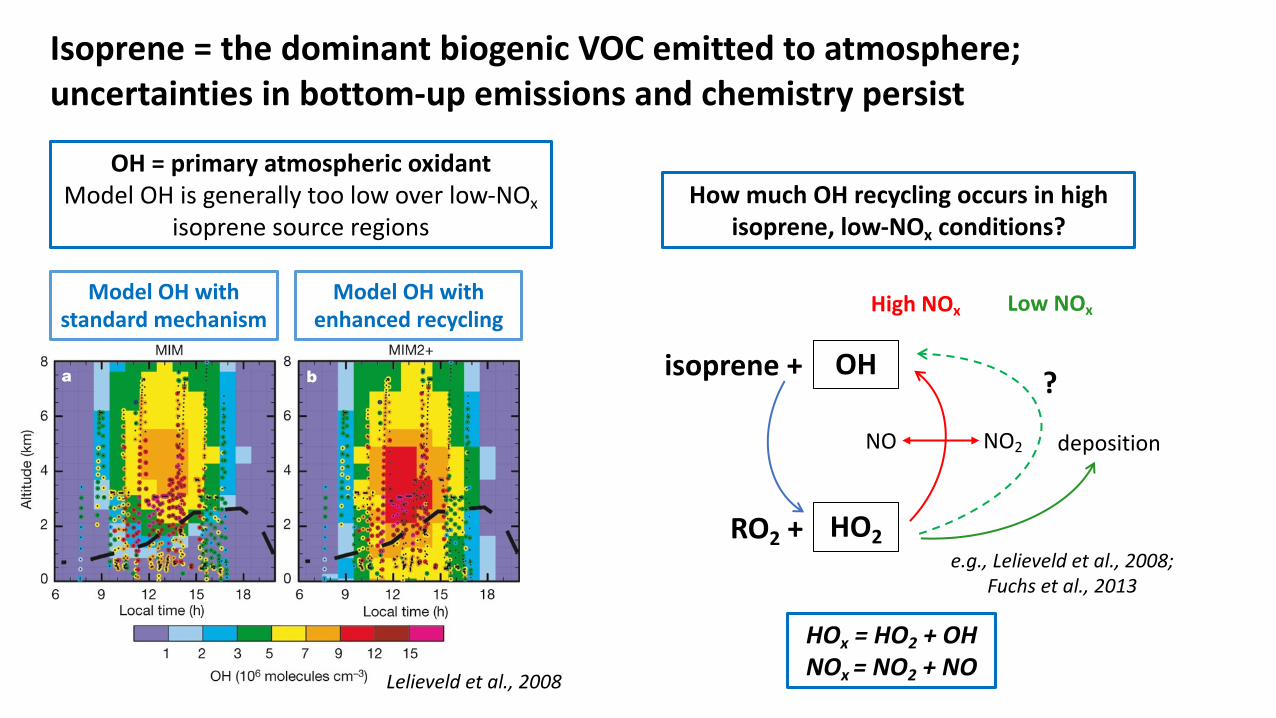
Isoprene = the dominant biogenic VOC emitted to atmosphere; uncertainties in bottom-up emissions and chemistry persist
535 570
150
Isoprene Methane Anth VOCs
Global Annual Emissions (Tg/yr)
Guenther et al., 2012
Bottom-up emissions sensitive to land cover, meteorology, canopy parametrization, etc.
Arneth et al., 2011
Same emission model & met data, different vegetation = 463 v 750 TgC/y
Observed Amazonia hotspots more localized than in GEOS-Chem
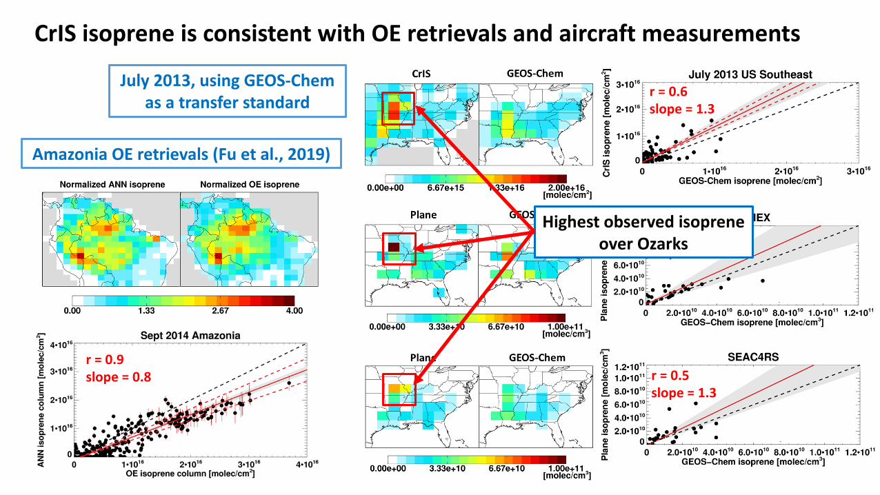
CrIS isoprene is consistent with OE retrievals and aircraft measurements
July 2013, using GEOS-Chem as a transfer standard
r = 0.6slope = 1.3
r = 0.7slope = 1.2
r = 0.5slope = 1.3
Highest observed isoprene over Ozarks
r = 0.9slope = 0.8
Amazonia OE retrievals (Fu et al., 2019)
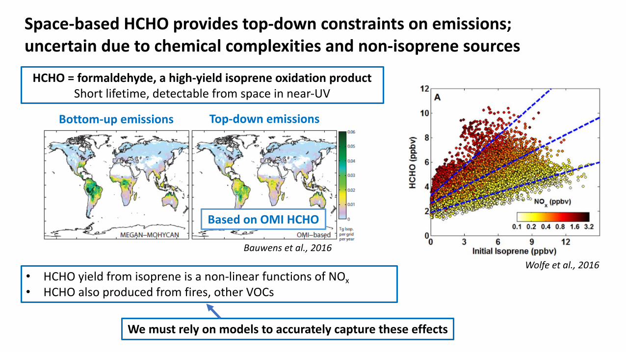
Space-based isoprene and HCHO provide combined constraints on emissions and chemistry in isoprene source regions
Isoprene column
GEOS-Chem, July 2013
Isoprene emissions (MEGANv2.1)
Isoprene BL lifetime
Isoprene column distribution distinct from that of emissions
Highest emissions
Highest columns
τ ~ 1h
τ > 12h
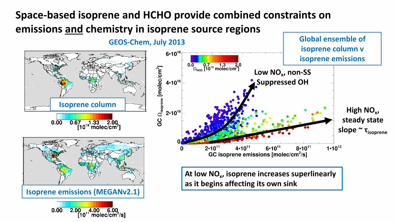
Space-based isoprene and HCHO provide combined constraints on emissions and chemistry in isoprene source regions
Isoprene column
Isoprene emissions (MEGANv2.1)
Isoprene BL lifetime
Isoprene column distribution distinct from that of emissions
Global ensemble of isoprene column v isoprene emissions
High NOx, steady state
slope ~ τisoprene
Low NOx, non-SSSuppressed OH
At low NOx, isoprene increases superlinearlyas it begins affecting its own sink
GEOS-Chem, July 2013
Space-based isoprene and HCHO provide combined constraints on emissions and chemistry in isoprene source regions
GEOS-Chem, July 2013
Isoprene emissions (MEGANv2.1)
HCHO is more buffered to OH variability:• Loss to photolysis still occurs at low OH• Loss proportional to [isoprene]×[OH]
Global ensemble of isoprene:HCHO column ratio v isoprene lifetime
r = 0.94
Isoprene column
Isoprene:HCHO ratio = proxy for atmospheric oxidation capacity in source regions
Space-based isoprene:HCHO ratio supports current model treatment of OH chemistry in isoprene source regions
CrIS isoprene:OMI HCHO GEOS-Chem isoprene:HCHO
GEOS-Chem-CrIS difference
Lowest model NO2 columns not seen in observations
Agreement within 10-40% at low-to-moderate NOx argues against
substantial missing OH recycling
OMI QA4ECV HCHO and NO2
Observed isoprene lifetime consistent with observed NO2 over Amazonia, large scale NOx bias evident in model
slope = 0.18
τisop = Ωisop:ΩHCHO/0.18
Measured lifetime agrees with chemical expectations = additional
confirmation of our approach
Large scale NOx bias likely due to underestimated soil NOx emissions (Liu et al., 2016)
A long-term record of isoprene from CrIS will give us new insights into interannual variability and chemistry-climate couplings
April 2012-October 2018
Onset of 2015/2016 El Niño = warmer temperatures,
drought stress?
Journal of Geophysical Research: Atmospheres 10.1002/2016JD024828
of an arbitrary spectrum y onto the NH3 spectral signature (a spectral Jacobian K corresponding to a change inNH3) resulting in a single pseudoquantitative number (called hereafter HRI, for “hyperspectral range index”):
HRI =KT S−1
y (y − y)√
KT S−1y K
, (1)
with y a mean background spectrum associated with Sy . Note that the HRI defined here is normalized suchthat it has a mean of zero and a standard deviation of 1 for spectra without observable quantities of NH3.When the HRI exceeds 3 or 4 (standard deviations) one can be reasonably confident that detectable NH3
are present in the observed scene. This method is derived from the main formula appearing in optimalleast squares estimates but turns out to be equivalent to the statistical method called “linear discriminationanalysis,” which is commonly used in classification problems [Clarisse et al., 2013]. The HRI detection method isfast and extremely sensitive (up to an order of magnitude more sensitive than brightness temperature differ-ence techniques), because very wide spectral ranges can be used and because it captures spectral correlationbetter than forward models can. A forward model is used only for the calculation of the Jacobian, but sinceJacobians are essentially spectral differences, the majority of the forward model errors cancel out. Thus, theerrors introduced to the HRI by the forward model are, in general, unimportant. As such, the detection methodavoids a lot of the problems of regular optimal estimation methods.
The HRI, a measure for the NH3 signature strength in the spectrum, is not only dependent on the amount ofNH3 but through the radiative transfer also on the thermal state of the atmosphere. The principal parameterhere is the thermal contrast defined as the temperature difference between the atmospheric boundary layerand the surface. For a fixed NH3 column, a larger thermal contrast (TC) will give rise to larger spectral signaturesand vice versa. HRIs can therefore be converted into reasonably accurate columns by taking into accountthe thermal contrast via two-dimensional lookup tables (LUT) mapping the pair (HRI, TC) to NH3 columns.A retrieval algorithm based on this idea was developed in Van Damme et al. [2014a], who also presented away to realistically estimate uncertainties for each measurement. The high sensitivity of this LUT-based HRImethod was apparent in this first study with the discovery of a large number of new highly localized hot spots,retrieval results for the evening overpass of IASI, and for the first time detection of NH3 transport over oceans.Quantitatively, the algorithm showed a good correlation with independent retrievals using optimal estima-tion techniques. These measurements were compared with the LOTOS-EUROS model output in Van Dammeet al. [2014b] and to in situ measurements in Van Damme et al. [2015a], and agreement was overall achievedwithin measurement uncertainty, although limitations of both models and in situ measurements were alsoexposed. These studies also highlighted the difficulties in comparing satellite measurements with models orin situ data and stressed the need to very carefully take into account the measurement uncertainties. They alsoexposed the following limitations of the LUT-based HRI method: (1) Using constant NH3 vertical profiles canintroduce potentially large errors (in Van Damme et al. [2014a], one fixed profile over land is used which peaksat the surface and one over oceans which peaks around 1400m). (2) While TC is taken into account, residualdependencies on, for instance, the complete temperature profile are not. (3) Instrumental noise causes a highbias of the measurements [Van Damme et al., 2015a], as a result of the fact that each HRI is always convertedinto a positive column. Especially for observations where the sensitivity to NH3 is low this can lead to drasticpositive mean biases (even if the associated estimated uncertainty on the individual observations are correct).
In this paper we propose an extension of the LUT-based HRI method from Van Damme et al. [2014a]. Insteadof using a two-dimensional LUT, we use here a feedforward neural network (NN) for the conversion of HRI toNH3 columns. A NN can approximate any (unknown or difficult to calculate) function Y = f (x) (under mildassumptions) by a transfer function F(W, x) which can be readily evaluated. The weights W of the functionF are obtained via training on a training set {yi = f (xi)} (see, e.g., Hadji-Lazaro et al. [1999] and Turquety et al.[2004] for earlier satellite retrieval schemes that used NNs). As both rely on a database of training data, a NNcan be seen as a generalization of a LUT. However, the important difference is that a LUT needs to store anoutput value for each combination of its input parameters, and the size of the LUT therefore grows exponen-tially with the dimension of the table. The great strength of a NN lies in its ability to cope with hundreds ofinput parameters, thereby offering a lot more flexibility than a two-dimensional LUT, while not requiring theexpensive and, in many cases, repetitive calculations of spectral fitting approaches. So rather than using TCas an input parameter, the NN allows use of the full temperature profile as input. Other input parameters thatwe will use are surface emissivity, surface temperature, the pressure and water vapor vertical profiles, satelliteviewing angle, and information on the vertical profile shape of NH3.
WHITBURN ET AL. NEW IASI-NH3 NN RETRIEVAL ALGORITHM 6583
Spectral Jacobian
Background spectral covariance
Mean background spectrum
Measured spectrum
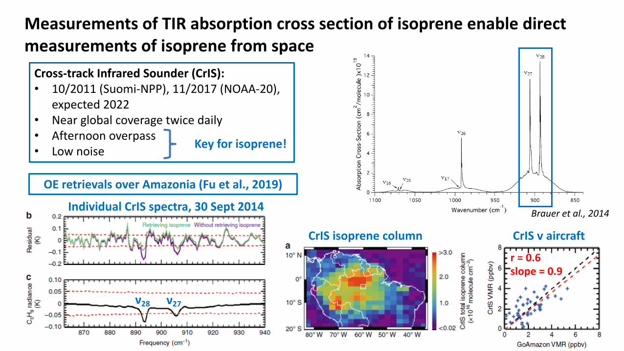
HRI uses full active spectral range for isoprene = enhanced sensitivity,
less subject to interferences
Next steps: next generation CrIS isoprene retrieval based on Hyperspectral Range Index (HRI) CrIS HRI looks more
“isoprene-like” than ΔTb
0.00 0.67 1.33 2.00
[1016 molec/cm2]
0.00 0.04 0.08 0.12
[K]
CrIS ΔTb CrIS HRI
[K]
CrIS isoprene
July 2013
Next steps: apply HRI-based retrieval to look at other species, advance understanding of VOC sources and chemistry-climate-ecosystem interactions
Species Primary SourcesMethanol Biosphere, biomass burning
Ethene Biosphere, biomass burning, vehicles
Ethyne Combustion
Acetone Biosphere, biomass burning
PAN Urban emissions, biomass burning
HCN Biomass burning
Acetic acid Biosphere, biomass burning
Ethane Natural gas, biofuel, biomass burning
Benzene Combustion
VOCs CO, O3, HCHO
SOA
OH, hν
Isoprene +
othersSimultaneous measurements of multiple VOCs from CrIS will provide
powerful new information to better understand biosphere-atmosphere interactions, biomass burning, and pollution across the globe!
Many thanks to:• Dejian Fu, Kevin Bowman, Evan Manning, Ruth Monarrez, Irina Strickland (JPL)• Chris Barnet (STC)• Matthew Alvarado, Karen Cady-Pereira, Daniel Gombos, Jennifer Hegarty (AER)• Eric Edgerton (SEARCH)• Stephen Springston (BNL)
• NASA ACMAP for funding
Science questions to be answered by long-term TIR sounder records
1) What does interannual variability tell us about the links between climate and VOC emission drivers?
2) How are VOC emissions (and OH!) changing over time?3) As anthropogenic emissions decrease in the US and elsewhere, how is atmospheric composition
changing?
We can do A LOT of science with even a weak signal! More species would be key to answering the below questions:
What should be the highest priorities for new trace gas products?
1) A greater suite of species active in TIR (not detectable with other sensors!) for doing detailed source apportionment globally over long timescales
2) Evaluation of sensitivity (AK) over different source types (biogenic versus biomass burning, etc)3) Near-real-time quick look-type product for specific events (e.g., large wildfires)
Species Primary SourcesMethanol Biosphere, biomass burning
Ethene Biosphere, biomass burning, vehicles
Ethyne Combustion
Acetone Biosphere, biomass burning
PAN Urban emissions, biomass burning
HCN Biomass burning
Acetic acid Biosphere, biomass burning
Ethane Natural gas, biofuel, biomass burning
Benzene Combustion
What are the key observational gaps?
1) Diurnal variability: net biogenic VOC emissions are high during the day and low (or negative!) at night; can we quantify emission processes from space versus just net emission strength?
2) Smaller footprints to look at fire impacts and urban plumes; more information about BVOC emissions as a function of plant type


![Evaluating the contribution of changes in isoprene emissions ...3 trends over the eastern United States, in light of current uncertainties in isoprene emissions and chemistry. [4]](https://static.documents.pub/doc/80x56/600324a3a13f5024f86c62ac/evaluating-the-contribution-of-changes-in-isoprene-emissions-3-trends-over-the.jpg)


