DOI: 10.1002/minf.201300172

Global Model for Octanol-Water Partition Coefficients fromProton Nuclear Magnetic Resonance SpectraNan An,[a] Farid Van Der Mei,[a] and Adelina Voutchkova-Kostal*[a]

1 Introduction

The octanol-water partition coefficient (logP) of a chemicalis the equilibrium ratio of concentrations between the octa-nol and water phases, which reflects its molecular hydro-phobicity. logP is a widely used physicochemical propertyin medicinal chemistry and toxicology.[1] Medicinal chemistsroutinely use logP to estimate oral[2] and skin[3] bioavailabil-ity of drug candidates, as well as build QSAR models, whileecotoxicologists and regulators use it to model acute andchronic toxicity to aquatic species[4,5] and potential for bio-accumulation.[6] Rules of thumb for designing minimallytoxic chemicals to aquatic species are also based on logP :for example, compounds with logP less than 2 are ca. 80 %more likely to have low acute and chronic toxicity to aquat-ic species.[7] logP is thus a ubiquitous property that is rou-tinely determined by chemists, toxicologists and regulators,and streamlined, accurate methods for its determinationare highly desirable.

A number of experimental techniques are available fordetermining logP : from the traditional shake-flaskmethod,[8] which requires extensive centrifugation, to themore modern methods involving HPLC,[9] microemulsionelectrokinetic chromatography,[10] and centrifugal partitionchromatography.[11] The modern methods are more conven-ient than the shake-flask method, but are limited to com-pounds with certain ranges of logP or pKa values, and canbe less reliable than the shake-flask method.[12] Someclasses of compounds, such as surfactants, pose a particularchallenge for certain methods. For example, the HPLCmethod for measurement of logP is not applicable to sur-

factants because their retention times on the chromatogra-phy column are also dependent on the surfactant’s prefer-ence for surfaces and interfaces.[13] Furthermore all of thesemethods require prior purification of the chemical.

To provide rapid and convenient methods for logP deter-mination several types of in-silico estimation methods havebeen developed.[14] The group contribution methods, forexample, use the relative contributions of molecular frag-ments or atoms to predict logP. The predictive power ofthe most commonly used group contribution tools, such asALOGP[15] , CLOGP[16] , ACD,[17] KOWWIN[18] is in the range of0.90–0.95 r2 based on training sets of up to 13 000 com-pounds.[19] Although very fast and accurate, these methodsoften show lower accuracy when externally validated (r2 :0.51–0.91),[23] which could be due to limitations in the ap-plicability domains to structures containing predefinedfragments. In addition, group contribution methods do nottake into account whole-molecule attributes, such as sur-face area, dipole moment and connectivity. Methods basedon multiple linear regressions of molecular topology de-scriptors overcome some of these challenges. For example,methods implemented in VLOGP[19b] employ electrotopo-

[a] N. An, F. Van Der Mei, A. Voutchkova-KostalChemistry Department, The George Washington UniversityWashington, DC 20052, USA*e-mail : avoutchkova@gwu.edu

Supporting information for this article is available on the WWWunder http://dx.doi.org/10.1002/minf.201300172.

Abstract : The ability to estimate chemical and physicalproperties from experimental spectra is highly desirable, asit eliminates the need for a priori knowledge of exactchemical structure and allows the property estimation ofmixtures. Here we report the proof of principle that a pre-dictive method for octanol-water partition coefficient (logP)based on 1H-NMR spectra in d3-chloroform is feasible andcan yield accuracy comparable to in silico logP models. TheSpectrometric Data-Activity Relationship (QSDAR) reportedpredicts logP of neutral organic chemicals using descriptorsderived only from 1H-NMR chemical shifts, integrations and

peak widths. Proton NMR spectra of 140 compounds withdiverse structures were used to construct a Multiple LinearRegression (MLR) and a Partial Least Squares (PLS) modelthat predicts logP. The optimized models were internallyvalidated by K-fold cross validation and leave-one-out vali-dation, and externally with a test set of 28 chemicals. Thesquared regression coefficients of prediction for the MLRand PLS regression models were 0.970 and 0.971 respec-tively, showing that the method allows accurate predictionof logP values exclusively from predicted 1H NMR spectra.

Keywords: Octanol-water partition · NMR · QSDAR · PLS · MLR

� 2014 Wiley-VCH Verlag GmbH & Co. KGaA, Weinheim Mol. Inf. 2014, 33, 286 – 292 286

Full Paper www.molinf.com

logical structure quantifiers derived from molecular topolo-gy and achieve r2 of 0.986 with rms of external validation of0.27. Other tools, such as Schrodinger’s QikProp,[20] use de-scriptors derived from Monte Carlo simulations and yieldrobust linear models for logP with broad applicability do-mains (r2 = 0.90, q2 = 0.89, rms = 0.55).[21] Lastly, methodsbased on free energies of solvation in water and octanol(Equation 1) also show great promise but are computation-ally expensive, especially for large molecules.[22]

log P ¼ fDG0S ðwaterÞ � DG0

S ðoctanolÞ g ð2:303RTÞ�1 ð1Þ

Most importantly, the aforementioned in silico estimationmethods require knowledge of the exact chemical struc-ture, which can be a challenge if there is an ambiguity inthe structure, or if the chemicals of interest exist as mix-tures, (e.g. surfactants and natural oils).

The use of descriptors derived from experimental spectraovercomes these challenges (i.e. does not require knowl-edge of exact structure, nor purification of the test chemi-cal), and offers a number of other advantages. For example,descriptors derived from NMR spectra can be directly infor-mative of electronic properties of a chemical. The diamag-netic term of the chemical shift is related to the electrostat-ic potential of the nucleus, while the paramagnetic term isrelated to the orbital configuration.[23] In addition to chemi-cal shift, peak shape can also be used to indicate hydrogenbond donation, which is important for predicting proper-ties and biological activity. Spectrometric Data-Activity Rela-tionship (QSDAR) models may also be able to overcomeerrors introduced by approximations of partial charges,structural conformation and dielectric constants necessaryfor in silico models. Finally, the data acquisition for QSDARsis non-destructive, and is applicable to mixtures.

These advantages of QSDARs have spurred increasing in-terest in development of predictive models for propertiesand biological activity. The reported studies fall into threecategories: those that exclusively use NMR (or other spec-tral) features, those that combine spectral features withstructure-based or property-based descriptors, and thosethat use chemical shift differences from NMR spectra ob-tained in different solvents. The models that rely solely onNMR spectra use a variety of techniques to convert thespectra into descriptors, and subsequently reduce thenumber of descriptors to optimize the final model. For ex-ample, Flumingnan et al have reported a Partial LeastSquares model that uses 13C chemical shifts to predictphysicochemical properties of gasoline.[24] Beger et al havedeveloped QSDAR models for binding to corticosteroidbinding globulin,[25] estrogen receptor,[26] aryl hydrocarbonreceptor[27] and aromatase enzyme.[28] Among models thatcombine spectral descriptors with ones derived from struc-ture, many employ the chemical shift of an atom commonto all compounds in a homologous series. Khadikar et al.have included chemical shifts of SO2NH2 protons in model-ing carbonic anhydrase inhibitory activity,[29] and average

13C chemical shift to model lipophilicity of 29 alcohols withadditional structural indicator parameters.[30] Verma andHansch have used select 1H and 13C NMR shifts as molecu-lar descriptors in models of bioactivity evaluation. Theyhave also employed chemical shift differences of 13C NMRin water and methanol as one of several descriptors usedto build a logP model.[31] However, the use of additional de-scriptors generated from structure eliminates the advantag-es of a model that can be applied when exact structure isambiguous.

The present work describes a QSDAR for estimation oflogP entirely from 1H Nuclear Magnetic Resonance (NMR)data, which would not require knowledge of exact struc-ture, nor purification of the test chemical. This method isnot intended to replace structure-based in silico models,but rather provide a valuable alternative route to estimat-ing logP, which may be especially useful when chemicalstructure is not clearly defined. Since NMR is routinely usedfor structure characterization, such a method can stream-line logP determination in the workflow of a syntheticchemist. Furthermore, the method is non-destructive and isin theory readily applicable to product mixtures, but this re-mains to be experimentally shown in future work. Themethod only requires knowledge of the absolute integra-tion of any one resonance. The integrations of the otherresonances can be calculated relative to this value.

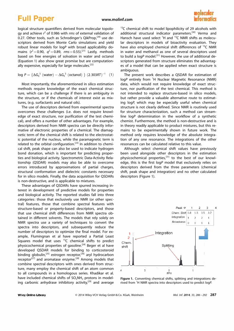
Although select chemical shift values have previouslybeen used alongside other descriptors in the estimationphysicochemical properties,[31] to the best of our knowl-edge, this is the first logP model that exclusively relies ondescriptors derived from the three parameters (chemicalshift, peak shape and integration) and no other calculateddescriptors (Figure 1).

Figure 1. Converting chemical shifts, splitting and integrations de-rived from 1H NMR spectra into descriptors used to predict logP.

� 2014 Wiley-VCH Verlag GmbH & Co. KGaA, Weinheim Mol. Inf. 2014, 33, 286 – 292 287

Full Paper www.molinf.com

2 Materials and Methods

2.1 Data Set

Experimental logP values for 168 compounds were ob-tained from ECOSAR EpiSuite.[29] The compounds were se-lected to represent 17 major functional classes with aliphat-ic and aromatic structural motifs (Figure 2). The selected

compounds thus represent a diverse dataset, with a molecu-lar weight range of 26 to 274 g/mol, a range of dipole mo-ments of 0 to 6.7 D, and a range of logP values between�1.51 to 9.95. These compounds are listed in Table 1. Thedata set was randomly divided into a training set of 140compounds, used for model generation, and a test set of28 compounds, used for validation. The logP range of thevalidation set is �1.36 to 8.65. The experimental logPvalues were used as the dependent variable.

2.2 Descriptor Generation and Preprocessing

Proton NMR spectra were predicted using MNova NMR Pre-dict v8 with CDCl3 as solvent and a 500 MHz magnetic field.The spectra were converted into [n � 4] matrices, where n isthe number of distinct resonances. The matrices containchemical shifts, integration and broadness (width at halfheight) for each of n proton resonances (Figure 1). A scriptin the R environment was used to generate a set of de-scriptors for each compound, which correspond to thenumber of protons with resonances in discrete chemicalshifts ranges.[32] For example, one descriptor corresponds to

the number of protons in the 0–1 ppm bin on a 500 MHzinstrument. The spectrum of 1–12 ppm was thus initiallysplit into 24 bins to generate the model.[38] Data pre-proc-essing included elimination of variables with near zero var-iance as well as any that have cross-correlations greaterthan 0.85.

2.3 MLR Model Generation

Multiple Linear Regression (MLR) models were developedin the R statistical environment.[33] MLR analyses were per-formed to fit the variables derived from NMR spectra to anequation of the following form:

log P ¼X

i

cixi þ b ð2Þ

where ci is the coefficient for each NMR-derived descriptorxi.

The full set of descriptors were used to generate an ini-tial MLR model, which was reduced in a stepwise mannerbased on the Akaike Information Criterion (AIC). AIC isa measure of relative quality of a statistical model and wasused to compare different models. Internal validation con-sisted of (1) Leave One Out algorithm, where each com-pound is systematically excluded from the training set andits logP is predicted by the model, and (2) K-fold cross vali-dation, where the data set is divided into K equal subsetsand each is systematically excluded from the training setand used as a test set.

2.4 PLS Model Generation

The Partial Least Squares regression, and its application toQSARs, has been described in detail in several excellent re-views.[34] The PLS model was selected because it is well-suited for data sets with a relatively large number of de-scriptors and leads to stable and highly predictive models,even when correlated descriptors are present. In brief, themethod assumes that X is the descriptor matrix of dimen-sions [a � b] , while Y[a] is the activity vector. The PLS re-gression reduces the large number of descriptors to a small-er number of orthogonal factors (latent variables). Thelatent variables are chosen to provide maximum correlationwith the dependent variables, which allows the use ofsmall number of factors in the final regression. X and Y aredecomposed into a two-matrix product plus residuals:

X ¼ TP0 þ E ð3Þ

Y ¼ UQ0 þ F ð4Þ

where matrices E and F contain the residuals for X and Y; Tand U are score matrices, and P’ and Q’ are loading matri-ces for X and Y respectively. The multiple regression modelcan be represented as:

Figure 2. Summary of the functional classes in the data set usedto build the model for predicting logP.

Table 1. Statistical model parameters obtained from MLR and PLSmodels.

Parameter MLR PLS

r2 0.949 0.954RMSE 0.484 0.438qext

2 0.971 0.970RMSEP 0.537 0.532Number of latent variables – 5Number of descriptors 13 –

� 2014 Wiley-VCH Verlag GmbH & Co. KGaA, Weinheim Mol. Inf. 2014, 33, 286 – 292 288

Full Paper www.molinf.com

Y ¼ XBþ G ð5Þ

where B is the matrix of regression coefficients.The PLS regression was implemented in the R statistical

environment.

2.5 Predictivity

The predictive power of each of the models was estimatedusing the coefficient of determination for predicted valuesof the validation set (qext

2) and the root mean square errorof prediction.

2.6 Benchmark Predictions of logP

Two well-established tools were used to obtain structure-based predictions of logP for the 168 compounds in themodel. The first is Schrodinger’s QikProp v. 3.0,[20] a validat-ed[35] property prediction software utilized extensively inthe field of drug discovery.[36] The second benchmarkmethod was KOWWIN (part of U.S. E. P. A.’s Estimation Pro-gram Interface Suite),[37] a program that estimates the logPusing an atom/fragment contribution method.[19c] The cur-rent KOWWIN model is based 13,058 compounds and is ex-tensively used and reviewed.[38]

3 Results and Discussion

3.1 Number of Spectral Bins Used for Model Generation

The first step in developing a QSDAR model is to identifya systematic way to generate descriptors from 1H NMRspectra. Our strategy was to derive two types of descrip-tors: one from the absolute integrations of proton reso-nance peaks that fall in distinct bins of the 1H spectrum,and two, from the relative broadness of the peaks in eachbin. We recognized that the number of bins (and thus thenumber of descriptors used) might have a profound impacton the model performance. Thus we varied the number ofbins from 5–26 and generated multivariate linear regression(MLR) models for each using peak integration and broad-ness descriptors. Figure 3 shows the relationship betweenthe number of spectral bins and model accuracy, estimatedby the adjusted coefficient of determination, (radj

2). The useof radj

2 allows us to take into account the spurious increasein r2 when additional explanatory variables are added tothe model. As shown in Figure 3, the radj

2, increases withnumber of bins, reaching an radj

2 value of 0.949 with 24bins. A further increase in the number of bins causes a de-crease in the radj

2, and as a result the optimal number ofbins was set at 24.

3.2 MLR Model Generation

The data set was divided randomly into a training set of140 compounds and a test set of 28 compounds. An initialfull MLR was built from the training set (radj

2 of 0.948). To

reduce this initial model we applied an iterative stepwiseprocedure based on minimization of AIC values. The AICprovides a useful way to balance the number of variableswith the goodness of fit of the reduced model.[39] This pro-cedure eliminated 15 of the variables, yielding a finalmodel with 13 variables. This final model is described inEquation 6, where xi corresponds to the consecutive pa-rameters obtained from absolute integrations of the spec-tral regions, and bn to the three broadness parameters. Themodel fits the Trophsa, Gramatica and Gombar criterion forratio of number of descriptors to number of data points.[41]

logP ¼ 0:229x0:5 þ 0:259x1 þ 0:234x1:5�0:074x2

þ 0:516x4:5 þ 0:322x5 þ 0:407x5:5 þ 0:381x6:5 þ 0:476x7

þ 0:270x7:5�1:494b1�2:198b2�0:538b3 þ 0:390

ð6Þ

r2 ¼ 0:949, radj2 ¼ 0:943, n ¼ 140, F ¼ 179:4

p-value : <2:2� 10�16, RMSE : 0:481:

K-fold cross validation (K = 10) was performed to internal-ly validate the model. This involves dividing the data setinto K subsets, and using each in turn to test the predictivepower of a model built from the remaining data set. Theaverage q2 of 10-fold cross validation was 0.944, with meanroot square error (RMSE) of 0.551. A leave-one-out (LOO)cross validation was also performed, which yielded a qLOO

2

of 0.946 and RMSE of 0.550. These metrics indicate that themodel shows consistent predictive power and robustness.Furthermore, the residuals were randomly distributed forthe predicted logP values (Figure 4 and Supporting Infor-mation Figure 2).

3.3 PLS Model Generation

In preparation for generating the PLS model the descriptorswere scaled and centered. The number of significant latentvariables was determined by the cross-validation method,which optimizes the residual standard error by the leave-one-out method. As shown in Figure 5, the number of

Figure 3. Number of spectral bins vs. model accuracy (adjusted r2)for the initial multivariate logP models.

� 2014 Wiley-VCH Verlag GmbH & Co. KGaA, Weinheim Mol. Inf. 2014, 33, 286 – 292 289

Full Paper www.molinf.com

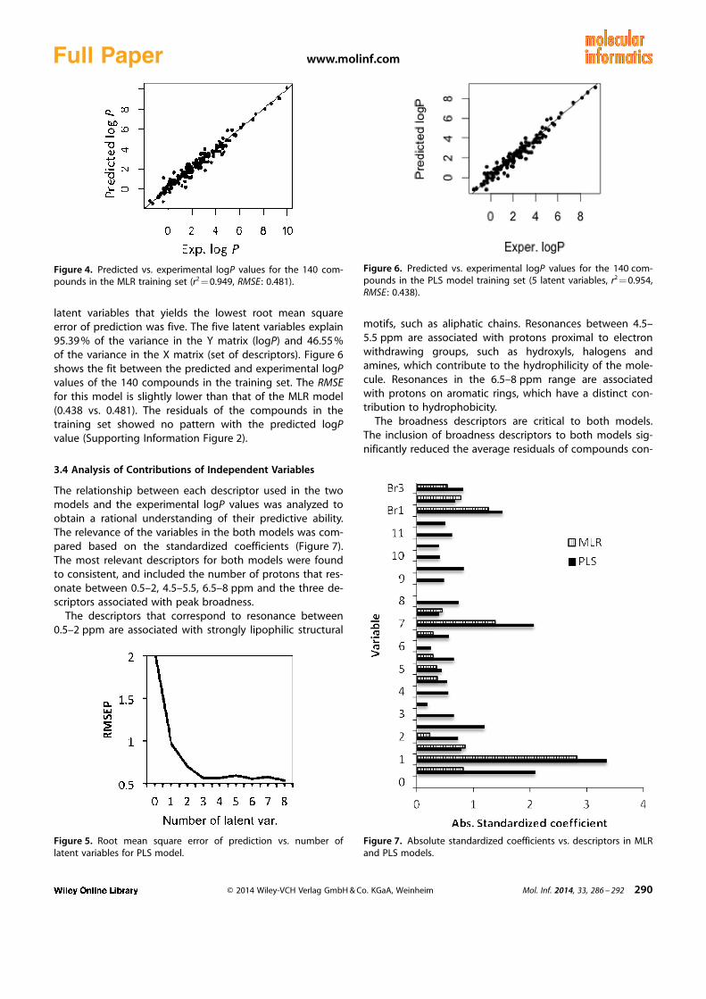
latent variables that yields the lowest root mean squareerror of prediction was five. The five latent variables explain95.39 % of the variance in the Y matrix (logP) and 46.55 %of the variance in the X matrix (set of descriptors). Figure 6shows the fit between the predicted and experimental logPvalues of the 140 compounds in the training set. The RMSEfor this model is slightly lower than that of the MLR model(0.438 vs. 0.481). The residuals of the compounds in thetraining set showed no pattern with the predicted logPvalue (Supporting Information Figure 2).

3.4 Analysis of Contributions of Independent Variables

The relationship between each descriptor used in the twomodels and the experimental logP values was analyzed toobtain a rational understanding of their predictive ability.The relevance of the variables in the both models was com-pared based on the standardized coefficients (Figure 7).The most relevant descriptors for both models were foundto consistent, and included the number of protons that res-onate between 0.5–2, 4.5–5.5, 6.5–8 ppm and the three de-scriptors associated with peak broadness.

The descriptors that correspond to resonance between0.5–2 ppm are associated with strongly lipophilic structural

motifs, such as aliphatic chains. Resonances between 4.5–5.5 ppm are associated with protons proximal to electronwithdrawing groups, such as hydroxyls, halogens andamines, which contribute to the hydrophilicity of the mole-cule. Resonances in the 6.5–8 ppm range are associatedwith protons on aromatic rings, which have a distinct con-tribution to hydrophobicity.

The broadness descriptors are critical to both models.The inclusion of broadness descriptors to both models sig-nificantly reduced the average residuals of compounds con-

Figure 4. Predicted vs. experimental logP values for the 140 com-pounds in the MLR training set (r2 = 0.949, RMSE : 0.481).

Figure 5. Root mean square error of prediction vs. number oflatent variables for PLS model.

Figure 6. Predicted vs. experimental logP values for the 140 com-pounds in the PLS model training set (5 latent variables, r2 = 0.954,RMSE : 0.438).

Figure 7. Absolute standardized coefficients vs. descriptors in MLRand PLS models.

� 2014 Wiley-VCH Verlag GmbH & Co. KGaA, Weinheim Mol. Inf. 2014, 33, 286 – 292 290

Full Paper www.molinf.com

taining amino, hydroxyl, alkyl halide and carboxylic acidgroups. These three descriptors identify protons involved inH/D exchange in deuterated solvents. H/D exchange canbe detected in 1H NMR spectra as broad peaks (width-at-half-height greater than ~75 Hz). Given that broadness alsodepends on concentration, pH and solvent, these factorsmust be controlled in spectral collection. Functional groupsthat exhibit H/D exchange, such as alcohols and amines,participate in hydrogen bonding (electrostatic intermolecu-lar interactions exhibited by molecules containing hydro-gen atoms bound to N, O or F). Hydrogen bonding increas-es water solubility and thus has a negative contribution tologP.[40]

3.5 Model Validation

The predictive power of the MLR and PLS models on thesame test set were compared, as shown in Figure 8 andTable 1. The maximum absolute residuals for the MLRmodel was 1.84 log units, compared to 1.04 for the PLSmodel, on a data set with experimental logP values in therange of �1.51 to 9.95. The external validation subset wasresampled 10 times from the 168-compound data set tocheck the consistency of both models. The average RMSEPfor the MLR model was 0.540, while that for the PLS model :0.531.

These data indicate that although the predictive per-formance of the two models was closely comparable, thatof the PLS model is slightly superior and more stable thanthe MLR model. However, this may change as the trainingset for the models is expanded to include greater structuraldiversity, which will populate any descriptor space that isnot utilized in this model, such as resonances between 8.0–8.5 ppm.

An analysis of predictive ability by functional class indi-cates that nitriles and alkynes (especially internal) have thehighest residuals. This is attributed to the lack of protonson the sp-hybridized carbons, which hinders the ability ofthe model to identify these functional groups. This issue

will be addressed by the inclusion of 13C-NMR spectral datainto the future model.

The applicability domain for this model can be conserva-tively defined by the structural diversity and defining prop-erties of the training set. As such, the applicability domainfor this model consists of compounds with molecularweight <450 Da, which have the functional groups shownin Figure 2, and have no more than 3 functional groupsper molecule.

3.6 Benchmarking to Structure-Based Models

This performance of the model was compared to two well-established methods for structure-based prediction –Schrçdinger’s QikProp[20] and EPI Suite KOWWIN[37] . ThelogP values of the 28 compounds in the external validationset were predicted with both programs. KOWWIN-predictedlogP values showed the highest correlation to experimentaldata (r2 = 0.987, RMSE = 0.234), while those from Qikprop:r2 = 0.959, RMSE : 0.421. The predictions obtained from ourmodel compare well to both of the structure-based tools(r2 = 0.970, residual standard error: 0.532). We note, howev-er, that both of the commercial packages used have beentrained on substantially larger training sets, and anticipatethat expansion of the training set will yield RMSEP valuesthat are even more favorably comparable with structure-based models.

4 Conclusions

This work demonstrates the proof-of-concept that 1H-NMRspectroscopic data can be used exclusively to builda robust model that predicts octanol-water partition coeffi-cient, one of the key properties used to estimate biologicalactivity of drugs and commodity chemicals. The ongoingwork in our laboratory to expand the training set, provideexternal validation with complex biologically-relevant mole-cules, incorporate 13C NMR data and replace the predictedwith experimental NMR spectra will further demonstratethe utility of such QSPRs.

Figure 8. Predicted vs. experimental logP values for 28 compounds in validation set predicted based on (a) MLR model (Equation 6) qext2 =

0.971, RMSEP : 0.537). (b) PLS model (qext2

=0.970, RMSEP = 0.532).

� 2014 Wiley-VCH Verlag GmbH & Co. KGaA, Weinheim Mol. Inf. 2014, 33, 286 – 292 291

Full Paper www.molinf.com

Acknowledgements

We would like to acknowledge Prof. Paul Anastas for the in-spiration of this work, as well as Prof. E. Arthur Robinson forhelpful discussions.

References

[1] A. Leo, C. Hansch, D. Elkins, Chem. Rev. 1971, 71, 525 – 616.[2] C. A. Lipinski, F. Lombardo, B. W. Dominy, P. J. Feeney, Adv.

Drug Deliv. Rev. 1997, 23, 3 – 25.[3] M. P. Edwards, D. A. Price, Annu. Rep. Med. Chem. 2010, 45,

381 – 391.[4] a) M. T. D. Cronin, Curr. Comput-Aid Drug 2006, 2, 405 – 413;

b) J. J. Ellington, F. E. Stancil, Environmental Research Labora-tory (Athens Ga.), Octanol/water partition coefficients for evalu-ation of hazardous waste land disposal : selected chemicals,U.S. Environmental Protection Agency, Environmental Re-search Laboratory, Athens, GA, 1988 ; p. 3.

[5] K. L. Kaiser, S. R. Esterby, Sci. Total Environ. 1991, 109–110,499 – 514.

[6] S. Bintein, J. Devillers, W. Karcher, SAR and QSAR in Environ-mental Research 1993, 1, 29 – 39.

[7] a) A. M. Voutchkova, J. Kostal, J. B. Steinfeld, J. Emerson, B. W.Brooks, P. Anastas, J. B. Zimmerman, Green Chem. 2011, 13,2373 – 2379; b) A. M. Voutchkova, J. Kostal, K. M. Connors,B. W. Brooks, P. Anastas, J. B. Zimmerman, Green Chem. 2012,14, 1001 – 1008; c) G. D. Veith, D. J. Call, L. T. Brooke, Can. J.Fisheries Aqu. Sci. 1983, 40, 743 – 748.

[8] C. Hansch, A. J. Leo, Exploring QSAR: Fundamentals and Appli-cations in Chemistry and Biology, American Chemical Society,Washington, DC, 1995.

[9] J. E. Haky, A. M. Young, J. Liq. Chromatogr. , 1984, 7, 675 – 689.[10] S. J. Gluck, M. H. Benko, R. K. Hallberg, K. Steele, J. Chromatogr.

A 1996, 744, 141 – 146.[11] a) R. A. Menges, G. L. Bertrand, D. W. Armstrong, J. Liq. Chro-

matogr. 1990, 13, 3061 – 3077; b) A. Berthod, Y. Han, D. W.Armstrong, J. Liq. Chromatogr. 1988, 11, 1441 – 1456.

[12] L. G. Danielsson, Y. H. Zhang, TrAC – Trends Anal. Chem. 1996,15, 188 – 196.

[13] H. Wiggins, A. Karcher, J. M. Wilson, I. Robb, “Determining Oc-tanol/Water Partitioning Coefficients for Industrial Surfactants”,in IPEC Conference, 2008.

[14] a) P. Buchwald, N. Bodor, Curr. Med. Chem. 1998, 5, 353 – 380;b) J. Sangster, Octanol-Water Partition Coefficients: Fundamen-tals and Physical Chemistry, Wiley, Chichester, 1997, p. 170.

[15] I. V. Tetko, V. Y. Tanchuk, J. Chem. Inf. Comp. Sci. 2002, 42,1136 – 1145.

[16] Pomona College and BioByte, I. CLOGP, Claremont, CA, 1988–2011.

[17] Advanced Chemistry Development, I. ACD/PhysChem Predictor,Version 10.00, http://www.acdlabs.com, Toronto, ON, Canada,2012.

[18] U. S. Environmental Protection Agency, KOWWIN, implement-ed in EPI Suite, 2000–2012.

[19] a) A. K. Ghose, V. N. Viswanadhan, J. J. Wendoloski, J. Phys.Chem. A 1998, 102, 3762 – 3772; b) V. K. Gombar, K. Enslein, J.

Chem. Inf. Comp. Sci. 1996, 36, 1127 – 1134; c) W. M. Meylan,P. H. Howard, J. Pharm. Sci. 1995, 84, 83 – 92.

[20] W. J. Jorgensen, QikProp, v. 3.0; Schrodinger, LLC, New York,NY, 2003.

[21] a) E. M. Duffy, W. L. Jorgensen, J. Am. Chem. Soc. 2000, 122,2878 – 2888; b) W. L. Jorgensen, E. M. Duffy, Med. Chem. Lett.2000, 10, 1155 – 1158.

[22] E. J. Delgado, J. Mol. Model. 2010, 16, 1421 – 1425.[23] J. W. Emsley, J. Feeney, L. H. Sutcliffe, High Resolution Nuclear

Magnetic Resonance Spectroscopy. , 1st ed. , Pergamon Press,Oxford, New York, 1965.

[24] D. L. Flumignan, R. Sequinel, R. R. Hatanaka, N. Boralle, J. E.de Oliveira, Energy Fuels 2012, 26, 5711 – 5718.

[25] R. D. Beger, J. G. Wilkes, J. Comput. Aid Mol. Des. 2001, 15,659 – 669.

[26] R. D. Beger, J. P. Freeman, J. O. Lay, J. G. Wilkes, D. W. Miller, J.Chem. Inf. Comp. Sci. 2001, 41, 219 – 224.

[27] R. D. Beger, J. G. Wilkes, J. Chem. Inf. Comp. Sci. 2001, 41,1322 – 1329.

[28] R. D. Beger, D. A. Buzatu, J. G. Wilkes, J. O. Lay, J. Chem. Inf.Comp. Sci. 2001, 41, 1360 – 1366.

[29] P. V. Khadikar, V. Sharma, S. Karmarkar, C. T. Supuran, Bioorg.Med. Chem. Lett. 2005, 15, 931 – 936.

[30] P. V. Khadikar, V. Sharma, R. G. Varma, Bioorg. Med. Chem. Lett.2005, 15, 421 – 425.

[31] R. P. Verma, C. Hansch, Chem. Rev. 2011, 111, 2865 – 2899.[32] A. Voutchkova-Kostal, N. An, F. Van Der Mei, Methods of Pre-

dicting Chemical Properties from Spectroscopic Data, Patent Ap-plication No. 61/836,430, 2013.

[33] R Programming Team, R: A Language and Environment forStatistical Computing, R Foundation for Statistical Computing,Vienna, Austria, 2009.

[34] a) K. L. Tang, T. H. Li, Anal. Chim. Acta 2003, 476, 85 – 92; b) T.Mehmood, K. H. Liland, L. Snipen, S. Saebo, Chemometr. Intell.Lab 2012, 118, 62 – 69; c) M. Hubert, K. Vanden Branden, J.Chemometr. 2003, 17, 537 – 549.

[35] L. Ioakimidis, L. Thoukydidis, A. Mirza, S. Naeem, J. Reynisson,QSAR Comb. Sci. 2008, 27, 445 – 456.

[36] E. H. Kerns, L. Di, Drug-like Properties: Concepts, StructureDesign and Methods : from ADME to Toxicity Optimization, Aca-demic Press, Amsterdam, 2008 ; p. 277.

[37] US EPA, Estimation Programs Interface Suite for Microsoft Win-dows, v 4.11, United States Environmental Protection Agency,Washington, DC, USA, 2013.

[38] EPA-SAB-07-11 Science Advisory Board Review of the Estima-tion Programs Interface Suite (EPI Suite), U.S.E.P.A. Office of theAdministrator, Report 2007.

[39] O. A. Raevsky, K. J. Schaper, J. K. Seydel, Quant. Struct.�Act.Relat. 1995, 14, 433 – 436.

[40] R. Gozalbes, J. P. Doucet, F. Derouin, Curr. Drug Target 2002, 2,93 – 102.

[41] A. Tropsha, P. Gramatica, V. K. Gombar, QSAR Comb. Sci. 2003,22, 69 – 77.

Received: December 2, 2013Accepted: February 3, 2014

Published online: April 15, 2014

� 2014 Wiley-VCH Verlag GmbH & Co. KGaA, Weinheim Mol. Inf. 2014, 33, 286 – 292 292

Full Paper www.molinf.com