Global Patterns in Green-up and Green-down

GLOBE® 2014 Global Patterns in Green-Up and Green-Down Learning Activity - 1 Biosphere

Appendix

Welcom

eIntroduction

ProtocolsLearning A

ctivitiesGlobal Patterns in Green-Up and Green-Down

PurposeTo investigate the annual cycle of plant growth and decline using visualizations and graphs

OverviewStudents will analyze visualizations and graphs that show the annual cycle of plant growth and decline. Students will explore patterns of annual change for the globe and each hemisphere in several regions that have different land cover and will match graphs that show annual green-up and green-down patterns with a specific land cover type. The activity begins with a class discussion and then students work in small groups and come together again to discuss their findings.

Student OutcomesAbility to use visualizations to analyze patterns Understanding relationships between visualizations and graphsAbility to describe global, hemispheric, and regional patterns of land cover growth

Science ConceptsPhysical Sciences

Sun is a major source of energy for changes on the Earth’s surface.

Earth and Space SciencesWeather changes from day to day and

over the seasons.Seasons result from variations in solar

insolation resulting from the tilt of the Earth’s rotation axis.

The sun is the major source of energy at Earth’s surface.

Life SciencesOrganisms can only survive in

environments where their needs are met.

Earth has many different environments that support different combinations of organisms.

Organisms’ functions relate to their environment.

Organisms change the environment in which they live.

Humans can change natural environments.

Plants and animals have life cycles.Ecosystems demonstrate the

complementary nature of structure and function.

All organisms must be able to obtain and use resources while living in a constantly changing environment.

Populations of organisms can be categorized by the function they serve in the ecosystem.

Sunlight is the major source of energy for ecosystems.

The number of animals, plants and microorganisms an ecosystem can support depends on the available resources.

Humans can change ecosystem balance.

Energy for life derives mainly from the sun.

Living systems require a continuous input of energy to maintain their chemical and physical organizations.

Scientific Inquiry AbilitiesAnalyzing visualizations for important

patterns in seasonal changeSolving a problem using data in a

visualizationComparing across multiple variablesUsing evidence from graphs and

visualizations to characterize ecosystems

Use appropriate tools and techniques.Develop explanations and predictions

using evidence.Recognize and analyze alternative

explanations.Communicate results and

explanations.

!?


Note: Similar skills for the local scale are taught in the GLOBE phenology protocols. The GLOBE training video Remote Sensing explains how scientists use remote sensing to determine land cover types.

TimeTwo 45-minute class periods

LevelMiddle, Secondary

MaterialsOverhead projector and transparencies

(4) or color visualization pagesScissors for students to shareWork Sheet (2 pages) and flip book

sheetWall map or atlas showing major

topographic regions

PreparationMake copies of the Work Sheets for all of the student groups. Students can work in groups: recommended group size is 2-3.

PrerequisitesExperience working with visualizations. See Learning to Use Visualizations: An Example with Elevation and Temperature and Draw Your Own Visualization (both in the Atmosphere Investigation), or the GLOBE Visualization tools on the GLOBE website. Ability to read an X-Y graph Familiarity with land cover types

BackgroundPlants have adapted their growth patterns to the local environment. Climate features such as temperature and amount of rainfall influence plant growth and dormancy. In many parts of the world, changes in plants can be observed as trees lose their leaves or sprout new growth. When plants sprout new growth we call it green-up; when they lose their leaves it is called green-down. Scientists study the seasonal cycles of plant growth to understand climate change. If climate conditions change, the length of plant growth cycles may differ from that observed in previous years. Vegetation vigor refers to the amount of growth that plants experience. The growing season is the period between spring growth (green-up) and fall decline (green-down). If global warming is occurring and affecting the Earth, scientists would expect to see earlier dates for spring green-up than in past years. Scientists study these changes using data from sensors on satellites that cover large regions of the Earth.Global patterns in green-up and green-down follow the annual climate cycle. This means that just as summer in the Northern Hemisphere occurs during winter in the

Southern Hemisphere, green-up happens in the North while green-down is happening in the South. The Northern Hemisphere experiences a more dramatic green-up and green-down than the Southern Hemisphere does. This trend also occurs with climate patterns; the Northern Hemisphere experiences much colder winters and hotter summers than the Southern Hemisphere does. The reason for this is that the Northern Hemisphere contains most of the land on Earth. Land is more easily heated and cooled than water.Vegetation vigor can be examined at a local level by observing the changes in vegetation that occur seasonally. The Phenology Protocols explore this by tracking changes in plant growth. In order to understand changes in vigor at a global level, satellite data must be used. This activity uses visualizations of vegetation vigor data that were collected by a sensor carried by a satellite. This sensor is called the Advanced Very High Resolution Radiometer (AVHRR) and is operated by the National Oceanic and Atmospheric Agency (NOAA). The vegetation vigor data collected by this sensor shows how much sunlight is being absorbed by plants for photosynthesis in contrast to the amount that is being reflected.


Appendix

Welcom

eIntroduction

ProtocolsLearning A

ctivities

Unfortunately, the AVHRR measurements of vegetation vigor are not precise: the resolution of the data is 1 square kilometer. It is important, then, for GLOBE students to help scientists understand how good the AVHRR measurements are by collecting local data using the Phenology Protocols. Visualizations of vegetation vigor help scientists understand how vegetation in different regions responds to the seasonal changes in weather. (Visualizations are combined with numerical data, in the form of a graph, of the average values per month.) Comparing vigor visualizations with ones showing different land covers in different regions can help scientists understand how different regions respond to the seasons.

What To Do and How To Do ItThis activity can take up to two class periods depending upon the amount of introduction given and the length of the class discussions.Day 1:Conduct a class discussion to orient students to the visualizations and conduct an initial analysis of the difference in vegetation vigor over a year and the relationship between land cover types and vegetation vigor.Day 2:Divide students into small groups to analyze data in order to classify regions based on the change in the vegetation vigor over the year and to answer the Work Sheet questions.Facilitate a class discussion during which the groups of students present their results and discuss the evidence they found for their conclusions.In preparation for the class discussion, make copies of the color visualizations shown in Figures BIO-GP-2 and BIO-GP-3. Color copies for printing onto transparencies or paper, or for projecting, can be obtained at the GLOBE website.Step 1. Class DiscussionThis activity uses both visualizations of data and graphs of data. Each visualization is based on a map of the continents. The first visualization, Figure BIO-GP-1a, shows categories of land cover expressed using

the MUC (Modified UNESCO Classification) System . For simplicity, some MUC classes are combined. The MUC classes of shrubland and barren land are represented as one class. All graminoid with trees classes (tall, medium-tall, and short) are also one category, Graminoid with Trees. Another MUC class, tropical mainly evergreen, is simply distinguished by its location: Tropical Forest. Finally, the MUC class Temperate Broad-leaved Deciduous is simply called Mixed Forest.Each class is shown in a different color: tropical forest (blue-green), cultivated land (orange), graminoid with trees (brown), graminoid (yellow), mixed forest (green), shrubland and barren land (tan), and tundra (gray). Students should be familiar with the plants that grow in these land cover types. For each land cover type, a corresponding value for vegetation vigor in January and July can be seen in Figures BIO-GP-2a and BIO-GP-2b, respectively.Initiate the class discussion by characterizing your local land cover type and discussing the seasonal changes observed in your local vegetation. How do different plants react to seasonal changes? Do all plants respond only to shorter daylight and colder temperatures? Do some react to periods of dryness? Discuss the major climate cycles in your area. Next, orient students to the visualizations shown in Figures BIO-GP-1 and BIO-GP-2 as described in detail below. Figures BIO-GP-2a and BIO-GP-2b illustrate the seasonal extremes of vegetation vigor by showing values during January and July. Figure BIO-GP-1b shows a visualization of the difference in vegetation vigor between January and July to show the amount of seasonal change. Refer back to Figure BIO-GP-1a to explain the observed seasonal variation by showing the type of land cover present in major regions.

Seasonal Extremes in January and July

1. Explain that the visualizations of vegetation vigor in Figure BIO-GP-2 are drawn using shades of green so that higher numeric values (which correspond to more vegetation) are darker shades. Vegetation vigor values in this visualization range from


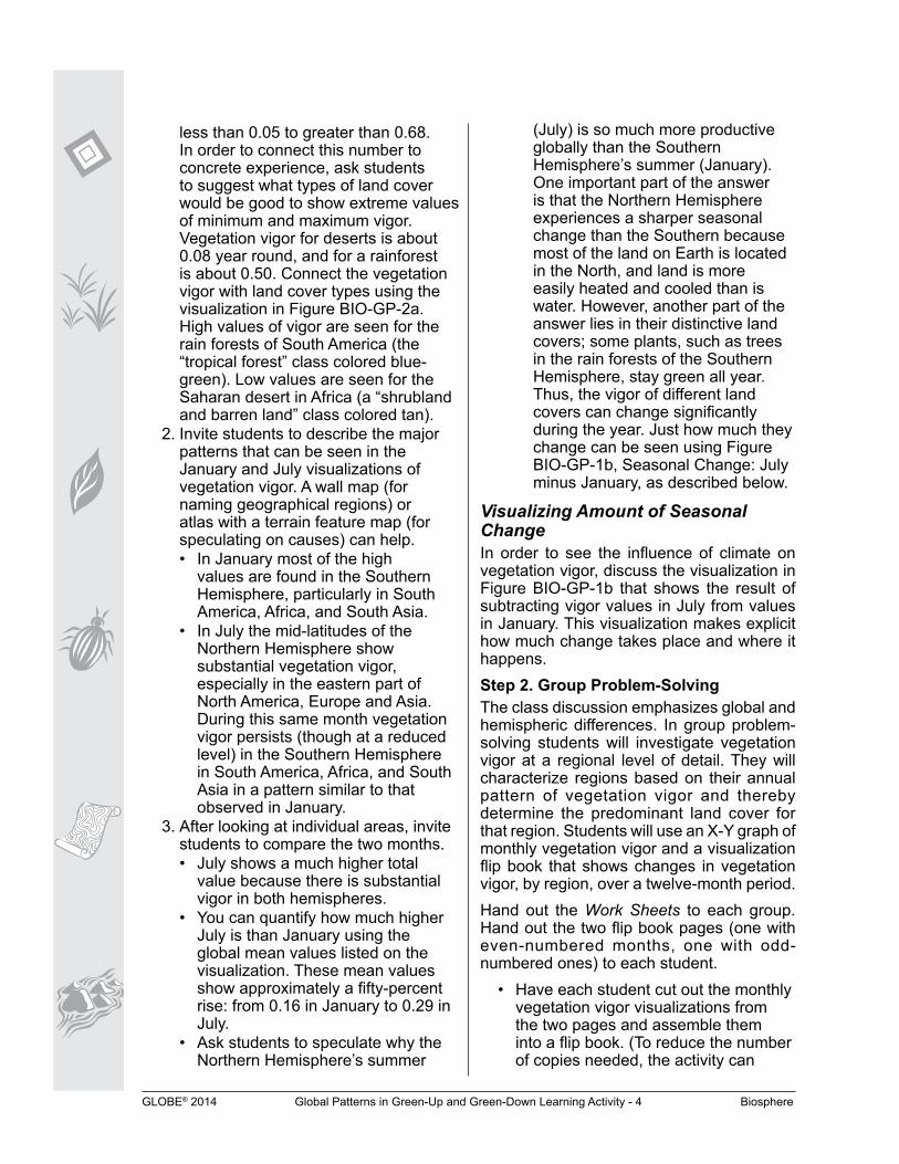
less than 0.05 to greater than 0.68. In order to connect this number to concrete experience, ask students to suggest what types of land cover would be good to show extreme values of minimum and maximum vigor. Vegetation vigor for deserts is about 0.08 year round, and for a rainforest is about 0.50. Connect the vegetation vigor with land cover types using the visualization in Figure BIO-GP-2a. High values of vigor are seen for the rain forests of South America (the “tropical forest” class colored blue-green). Low values are seen for the Saharan desert in Africa (a “shrubland and barren land” class colored tan).

2. Invite students to describe the major patterns that can be seen in the January and July visualizations of vegetation vigor. A wall map (for naming geographical regions) or atlas with a terrain feature map (for speculating on causes) can help.

• In January most of the high values are found in the Southern Hemisphere, particularly in South America, Africa, and South Asia.

• In July the mid-latitudes of the Northern Hemisphere show substantial vegetation vigor, especially in the eastern part of North America, Europe and Asia. During this same month vegetation vigor persists (though at a reduced level) in the Southern Hemisphere in South America, Africa, and South Asia in a pattern similar to that observed in January.

3. After looking at individual areas, invite students to compare the two months.

• July shows a much higher total value because there is substantial vigor in both hemispheres.

• You can quantify how much higher July is than January using the global mean values listed on the visualization. These mean values show approximately a fifty-percent rise: from 0.16 in January to 0.29 in July.

• Ask students to speculate why the Northern Hemisphere’s summer

(July) is so much more productive globally than the Southern Hemisphere’s summer (January). One important part of the answer is that the Northern Hemisphere experiences a sharper seasonal change than the Southern because most of the land on Earth is located in the North, and land is more easily heated and cooled than is water. However, another part of the answer lies in their distinctive land covers; some plants, such as trees in the rain forests of the Southern Hemisphere, stay green all year. Thus, the vigor of different land covers can change significantly during the year. Just how much they change can be seen using Figure BIO-GP-1b, Seasonal Change: July minus January, as described below.

Visualizing Amount of Seasonal ChangeIn order to see the influence of climate on vegetation vigor, discuss the visualization in Figure BIO-GP-1b that shows the result of subtracting vigor values in July from values in January. This visualization makes explicit how much change takes place and where it happens.Step 2. Group Problem-SolvingThe class discussion emphasizes global and hemispheric differences. In group problem-solving students will investigate vegetation vigor at a regional level of detail. They will characterize regions based on their annual pattern of vegetation vigor and thereby determine the predominant land cover for that region. Students will use an X-Y graph of monthly vegetation vigor and a visualization flip book that shows changes in vegetation vigor, by region, over a twelve-month period.Hand out the Work Sheets to each group. Hand out the two flip book pages (one with even-numbered months, one with odd-numbered ones) to each student.

• Have each student cut out the monthly vegetation vigor visualizations from the two pages and assemble them into a flip book. (To reduce the number of copies needed, the activity can


Land CoverType

Tropical Forest

Cultivated Land

Graminoid with Trees

Graminoid

Mixed Forest

Shrubs, Desert,and Bare Ground

Tundra

Tropic of Cancer

Equator

Tropic of Capricorn

Tropic of Cancer

Equator

Tropic of Capricorn

Seasonal Change:

July minusJanuary

0 0.4 0.70.4-0.7

Figure BIO-GP-1a: Land Cover Type

Figure BIO-GP-1b: Seasonal Change: July Minus January


< 0.05 > 0.660.360.20 0.51

Vegetation Vigor

January, 1987

Vegetation Vigor

July, 1987

Mean value for January: 0.16Mean value for July: 0.29

VegetationVigor (NDVI)

Tropic of Cancer

Equator

Tropic of Capricorn

Tropic of Cancer

Equator

Tropic of Capricorn

Figure BIO-GP-2b: Vegetation Vigor, July, 1987

Figure BIO-GP-2a: Vegetation Vigor, January, 1987


Appendix

Welcom

eIntroduction

ProtocolsLearning A

ctivities

be completed using only one of the pages, showing every other month.)

• Students will use the vegetation vigor flip book to look at change over time in specific regions. The shades of gray in the flip book correspond to values on the graph. The students’ task is to extract information from the graph and combine it with both the flip book information and land cover descriptions to determine which land cover type goes with which graph.

• The Work Sheet asks students to explain their choice. Ask students to be sure to use evidence from the flip book and land cover descriptions in their explanations.

Step 3. Group PresentationsBring the students back together for a discussion of the results. Emphasize the important differences between the ecosystem dynamics of the regions, and suggest factors that might affect differences in vigor for different land covers. As students present their answers, watch for opportunities to hone their abilities to present ideas with sufficient justification. While students are characterizing regions, it is easy for them to focus only on finding the right answer (perhaps by using a

process of elimination) and to not think about the reason they were able to determine the land cover type. When the students engage in discussion about their answers, they need to provide good evidence of why their answer is correct.

Further InvestigationsThe global occurrence of green-up and green-down causes an annual fluctuation in the amount of carbon in the atmosphere. This fluctuation occurs because vegetation—like all forms of life on Earth—is made partly of carbon. When plants grow, they take carbon dioxide out of the atmosphere. When plants decay, they release carbon dioxide into the atmosphere. If the amount of vegetation declines, less carbon dioxide is removed from the atmosphere. The graph in Figure BIO-GP-3 shows atmospheric carbon dioxide per month for 3 years. Although the measurement is taken from only one location, it provides a global measure because of efficient mixing within the atmosphere. There are a number of interesting patterns to explore in this graph. Why is the decline so much faster than the rise? Why is the peak value of each succeeding year higher than that in the previous one?

Figure BIO-GP-3: Atmospheric Carbon Dioxide Concentration, Mauna Loa Observatory, Hawaii


ResourcesYou can analyze a large number of vegetation vigor visualizations using the GLOBE Visualization Server. The “Image Spreadsheet” option allows these visualizations to be further analyzed in relationship to other variables (e.g., temperature). The GLOBE Earth System posters (available on the GLOBE website) provide examples of image spreadsheets of this sort in which vegetation vigor (NDVI) is contrasted with several other climatic variables. Finally, see the Match the Biome activity on the GLOBE website. This activity asks students to connect climatic diagrams showing temperature and precipitation with land covers depicted in photographs.


Global Patterns in Green-Up and Green-DownWork Sheet

Names: _________________________________________________________________

Directions: Name the Land CoverThis activity will help you investigate vegetation vigor at a regional level. You will use an X-Y graph of monthly vegetation vigor and a visualization flip book that shows changes in vegetation vigor, by region, over a twelve-month period. From the graph, you will find the months in which each region has its growing season and how much the vegetation grows compared to other regions. You will then match the data from the X-Y graph to the vegetation vigor visualization in order to name the dominant land cover for that region.

1. Assemble the vegetation vigor flip book by cutting out each month and putting the pages in order from January to December. Using the Land Cover Locations map, look at how each region changes throughout the year. To begin, pick one region and one month, and use the flip book scale to determine the value of vigor in that month for that region. Repeat this for each region.

2. There are text descriptions of the land covers that you can use to understand how the vegetation changes in the map areas over one year.

3. Each line on the Vegetation Vigor graph represents one of the land cover locations. Your task is to name the land cover that each line corresponds to using data from the graph, the land cover descriptions, and the flip book. Use the following steps to do this.

Maximum and Minimum Vegetation Vigor: For each line on the graph, find the months in which the maximum and minimum values of vegetation vigor occur. Estimate the value of vigor in those months to the nearest 0.05. Record your results. You can get a clue to the answer using the flip book and its scale. For the maximum value you recorded, find that shade on the flip book scale and try to locate it in one of the regions.

Change: Another clue comes from the amount of change in the vigor over the year. Look at how much the line changes or stays level. Compute the value of the change in vigor by subtracting minimum vegetation vigor from the maximum value. Look again at the flip book. Which regions change a lot over the months? Which stay the same?

Growing Season: Knowing when a dramatic change occurs, such as green-up or green-down, can help you name the land cover. The graph shows the months of green-up and green-down: look for months in which the vegetation vigor value starts to increase from a low value (green-up) and decrease from a high value (green-down). Record the values you find for green-up and green-down.

Land Cover: Now you have enough clues to name the land cover. Be sure to explain your choice using evidence from the clues. Describe the clues from the graph, the flip book, and the land cover description.


Symbol Maximum Vegetation Vigor

MinimumVegetation Vigor

Change Growing Season

Month:Value:

Month:Value:

Land Cover: Explanation:




Month:Value:

Month:Value:





Month:Value:

Month:Value:





Month:Value:

Month:Value:





Month:Value:

Month:Value:



Land

Cov

er

Loca

tions

Equ

ator

Tund

ra Des

ert

Nor

th A

frica

nG

ram

inoi

d w

ith T

rees

Sou

th A

frica

nG

ram

inoi

d w

ith T

rees

Trop

ical

For

est

Vege

tatio

n Vi

gor

Vegetation Vigor

Janu

ary

Febru

ary

March

April

May

June

Ju

ly

Augus

t Septem

ber

Octobe

r

Novem

ber

Decem

ber

0.10

0.20

0.30

0.40

0.50

Flip

Boo

k S

cale

: Ve

geta

tion

Vigo

r (N

DV

I) Va

lue

0.05

0.36

0.66

Land

Cov

er D

escr

iptio

ns

Tund

ra: H

igh

latit

ude

treel

ess

plai

ns th

at o

ccur

in h

arsh

cl

imat

es o

f low

rain

fall

and

low

ave

rage

tem

pera

ture

.

Trop

ical

For

est:

Trop

ical

latit

ude

ecos

yste

m d

omin

ated

by

bro

adle

af e

verg

reen

tree

s.

Des

ert:

Eco

logy

lim

ited

by e

xtre

mel

y lo

w a

nnua

l rai

nfal

l an

d sp

arse

, low

veg

etat

ion.

Nor

th A

fric

an G

ram

inoi

d w

ith T

rees

: A m

oder

atel

y dr

y ec

osys

tem

dom

inat

ed b

y gr

assl

ands

and

sm

all t

rees

.

Sout

h A

fric

an G

ram

inoi

d w

ith T

rees

: A m

oder

atel

y dr

y ec

osys

tem

dom

inat

ed b

y gr

assl

ands

and

sm

all t

rees

.

Glo

bal G

reen

-Up

and

Gre

en-D

own

Wor

k S

heet

N

ames

: ___

____

____

____

___


1Ja

nuar

y

Vege

tatio

n Vi

gor

(ND

VI) 3

Mar

ch

Vege

tatio

n Vi

gor

(ND

VI)

5 May

Vege

tatio

n Vi

gor

(ND

VI)

7 July

Vege

tatio

n Vi

gor

(ND

VI) 9

Sep

tem

ber

Vege

tatio

n Vi

gor

(ND

VI)

11N

ovem

ber

Vege

tatio

n Vi

gor

(ND

VI)

Wor

k S

heet

: Odd

Mon

ths


2Fe

brua

ry

Vege

tatio

n Vi

gor

(ND

VI)

4 Apr

il

Vege

tatio

n Vi

gor

(ND

VI)

6Ju

ne

Vege

tatio

n Vi

gor

(ND

VI)

8

Aug

ust

Vege

tatio

n Vi

gor

(ND

VI) 10

Oct

ober

Vege

tatio

n Vi

gor

(ND

VI)

12D

ecem

ber

Vege

tatio

n Vi

gor

(ND

VI)

Wor

k S

heet

: Eve

n M

onth

s


Global Patterns in Green-Up and Green-DownRubric

For each criterion, evaluate student work using the following score levels and standards.

3 = Shows clear evidence of achieving or exceeding desired performance2 = Mainly achieves desired performance1 = Achieves some parts of the performance, but needs improvement0 = Answer is blank, entirely arbitrary or inappropriate

1. Fill out the table with observations from the X-Y graph for maximum vegetation vigor, minimum vegetation vigor, change, and growing season.

Score Level

Description

3 The table is filled out with correct observations from the graph (see student example). For some, such as the darkened triangles (third row) and empty triangles (fourth row), there is little distinction between the maximum and minimum values, or, as with the darkened circles (bottom row) the minimum values are all similar. In these cases there is no one correct answer. A student may select one of these similar months for a low or a high, but the key point is that they identify a very small value for Change.

2 The table is completely filled out. Most of the values are correct. Student may not have rounded the numbers correctly.

1 Table is mainly filled out. Many of the values are correct or close to correct.

0 Table not filled out, too sloppy to read, or the majority of the values are arbitrary.


2. Complete the table with observations from the graph, table and flip book (score individually for each land cover assignment).

Score Level

Description

3 The land cover is correctly filled out and the explanation provides a complete evidence-based justification: it describes the line in the graph, references the land cover in the flip book, and makes a comparison to other land covers/lines or offers other explanations of why this is a sensible choice.

2 The land cover is correctly filled out but the explanation provides only partial justification of the choice or provides logical justification without evidence from the materials consulted. Alternatively, the chosen land cover is incorrect, but the explanation provides a reasonable justification for the selection.

1 The land cover is incorrectly filled out and the explanation is present but insufficient, offering minimal evidence or logical argument.

0 Land cover is not filled out, or is incorrect. Logical explanation is omitted.





Month: SeptemberValue: 0.50

Month: JanuaryValue: 0.25

0.25 January to September

Land Cover:North African

Graminoidwith Trees

Explanation: This one is pretty much the opposite of the South African graminoid with trees, and it is the only one that gets as dark as the tropical forest in the flip book. It has its summer when North America has its summer, so it gets greenest in that hemisphere’s summer (June-Sept).




Month: JanuaryValue: 0.05

Month: MayValue: 0.05

0.0 There isn’t really one.

Land Cover: Desert

Explanation: This is the only one on the flip book that stays white all year long. This means that the values are really low all year, probably because there isn’t very much vegetation to grow. It is really low on the graph too. It is probably higher than the tundra for part of the year because it does have something growing in the winter, while the tundra is ice.




Month: JulyValue: 0.50

Month: SeptemberValue: 0.45

0.05 October to July

Land Cover: Tropical Forest

Explanation: This one has the highest overall values and it stays very high all year in the flip book and the graph. It is the highest (almost) all year in the graph. This makes sense since it is near the equator so it doesn’t get summers or winters.




Month: MarchValue: 0.45

Month: AugustValue: 0.20

0.25 September to March

Land Cover:South African

Graminoidwith Trees

Explanation: This is the only one with its peak is in the Southern Hemisphere’s summer, so it has to be in the Southern Hemisphere. The flip book also shows this area as getting dark (high vegetation vigor) during January to March. It also stays pretty dark all year (compared to the desert). It is the opposite of the North African graminoid with trees line.




Month: AugustValue: 0.30

Month: January, DecemberValue: 0.0

0.30 April to August

Land Cover: Tundra

Explanation: This line has the largest change of all the lines. It has no vegetation vigor until April (it is white in the flip book), then it gets very dark very quickly, then turns white again. This makes sense for it to be so far north, because the growing season there is very short. Its highest value never reaches as high as the tropical forest, and for the time that it is very high (July, August), it is darker in the flip book than the South African graminoid with trees

Date post:	01-Feb-2022
Category:	Documents
Upload:	others
View:	0 times
Download:	0 times

Global Patterns in Green-up and Green-down

Documents