GLOBAL REGULARITY FOR SOME CLASSES OF LARGE SOLUTIONS TO THE NAVIER-STOKES EQUATIONS JEAN-YVES CHEMIN, ISABELLE GALLAGHER, AND MARIUS PAICU Abstract. In [4]-[6] classes of initial data to the three dimensional, incompressible Navier- Stokes equations were presented, generating a global smooth solution although the norm of the initial data may be chosen arbitrarily large. The main feature of the initial data considered in [6] is that it varies slowly in one direction, though in some sense it is “well prepared” (its norm is large but does not depend on the slow parameter). The aim of this article is to generalize the setting of [6] to an “ill prepared” situation (the norm blows up as the small parameter goes to zero). As in [4]-[6], the proof uses the special structure of the nonlinear term of the equation. 1. Introduction We study in this paper the Navier-Stokes equation with initial data which are slowly varying in the vertical variable. More precisely we consider the system ∂ t u + u ·∇u - Δu = -∇p in R + ×Ω div u =0 u| t=0 = u 0,ε , where Ω = T 2 × R (the choice of this particular domain will be explained later on) and u 0,ε is a divergence free vector field, whose dependence on the vertical variable x 3 will be chosen to be “slow”, meaning that it depends on εx 3 where ε is a small parameter. Our goal is to prove a global existence in time result for the solution generated by this type of initial data, with no smallness assumption on its norm. 1.1. Recollection of some known results on the Navier-Stokes equations. The math- ematical study of the Navier-Stokes equations has a long history, which we shall describe briefly in this paragraph. We shall first recall results concerning the main global wellposedness re- sults, and some blow-up criteria. Then we shall concentrate on the case when the special algebraic structure of the system is used, in order to improve those previous results. To simplify we shall place ourselves in the whole euclidian space R d or in the torus T d (or in variants of those spaces, such as T 2 × R in three space dimensions); of course results exist in the case when the equations are posed in domains of the euclidian space, with Dirichlet boundary conditions, but we choose to simplify the presentation by not mentioning explicitly those studies (although some of the theorems recalled below also hold in the case of domains up to obvious modifications of the statements and sometimes much more difficult proofs). Key words and phrases. Navier-Stokes equations, global wellposedness. 1
Transcript
GLOBAL REGULARITY FOR SOME CLASSES OF LARGE SOLUTIONSTO THE NAVIER-STOKES EQUATIONS
JEAN-YVES CHEMIN, ISABELLE GALLAGHER, AND MARIUS PAICU
Abstract. In [4]-[6] classes of initial data to the three dimensional, incompressible Navier-Stokes equations were presented, generating a global smooth solution although the normof the initial data may be chosen arbitrarily large. The main feature of the initial dataconsidered in [6] is that it varies slowly in one direction, though in some sense it is “wellprepared” (its norm is large but does not depend on the slow parameter). The aim of thisarticle is to generalize the setting of [6] to an “ill prepared” situation (the norm blows up asthe small parameter goes to zero). As in [4]-[6], the proof uses the special structure of thenonlinear term of the equation.
1. Introduction
We study in this paper the Navier-Stokes equation with initial data which are slowly varyingin the vertical variable. More precisely we consider the system
∂tu+ u · ∇u−∆u = −∇p in R+×Ωdiv u = 0u|t=0 = u0,ε,
where Ω = T2×R (the choice of this particular domain will be explained later on) and u0,ε
is a divergence free vector field, whose dependence on the vertical variable x3 will be chosento be “slow”, meaning that it depends on εx3 where ε is a small parameter. Our goal is toprove a global existence in time result for the solution generated by this type of initial data,with no smallness assumption on its norm.
1.1. Recollection of some known results on the Navier-Stokes equations. The math-ematical study of the Navier-Stokes equations has a long history, which we shall describe brieflyin this paragraph. We shall first recall results concerning the main global wellposedness re-sults, and some blow-up criteria. Then we shall concentrate on the case when the specialalgebraic structure of the system is used, in order to improve those previous results.
To simplify we shall place ourselves in the whole euclidian space Rd or in the torus Td (orin variants of those spaces, such as T2×R in three space dimensions); of course results existin the case when the equations are posed in domains of the euclidian space, with Dirichletboundary conditions, but we choose to simplify the presentation by not mentioning explicitlythose studies (although some of the theorems recalled below also hold in the case of domainsup to obvious modifications of the statements and sometimes much more difficult proofs).
Key words and phrases. Navier-Stokes equations, global wellposedness.
1
2 J.-Y. CHEMIN, I. GALLAGHER, AND M. PAICU
1.1.1. Global wellposedness and blow-up results. The first important result on the Navier-Stokes system was obtained by J. Leray in his seminal paper [21] in 1933. He proved that anyfinite energy initial data (meaning square-integrable data) generates a (possibly non unique)global in time weak solution which satisfies an energy estimate; he moreover proved in [22]the uniqueness of the solution in two space dimensions. Those results use the structure ofthe nonlinear terms, in order to obtain the energy inequality. He also proved the uniquenessof weak solutions in three space dimensions, under the additional condition that one of theweak solutions has more regularity properties (say belongs to L2(R+;L∞): this would nowbe qualified as a “weak-strong uniqueness result”). The question of the global wellposednessof the Navier-Stokes equations was then raised, and has been open ever since. We shall nowpresent a few of the historical landmarks in that study.
The Fujita-Kato theorem [10] gives a partial answer to the construction of a global uniquesolution. Indeed, that theorem provides a unique, local in time solution in the homogeneousSobolev space H
d2−1 in d space dimensions, and that solution is proved to be global if the
initial data is small in Hd2−1 (compared to the viscosity, which is chosen equal to one here
to simplify). The result was improved to the Lebesgue space Ld by F. Weissler in [32] (seealso [13] and [16]). The method consists in applying a Banach fixed point theorem to theintegral formulation of the equation, and was generalized by M. Cannone, Y. Meyer and F.Planchon in [1] to Besov spaces of negative index of regularity. More precisely they proved
that if the initial data is small in the Besov space B−1+ d
pp,∞ (for p <∞), then there is a unique,
global in time solution. Let us emphasize that this result allows to construct global solutionsfor strongly oscillating initial data which may have a large norm in H
d2−1 or in Ld. A typical
example in three space dimensions is
uε0(x) def= ε−α sin(x3
ε
)(−∂2ϕ(x), ∂1ϕ(x), 0
),
where 0 < α < 1 and ϕ ∈ S(R3; R). This can be checked by using the definition of Besovnorms:
∀s > 0, ∀(p, q) ∈ [1,∞], ‖f‖B−sp,q
def=∥∥∥t s
2 ‖et∆f‖Lp
∥∥∥Lq(R+; dt
t).
More recently in [17], H. Koch and D. Tataru obtained a unique global in time solution fordata small enough in a more general space, consisting of vector fields whose components arederivatives of BMO functions. The norm in that space is given by
(1.1) ‖u0‖2BMO−1def= sup
t>0t‖et∆u0‖2L∞ + sup
x∈Rd
R>0
1Rd
∫P (x,R)
|(et∆u0)(t, y)|2dy,
where P (x,R) stands for the parabolic set [0, R2]×B(x,R) while B(x,R) is the ball centeredat x, of radius R.
One should notice that spaces where global, unique solutions are constructed for small initialdata, are necessarily scaling-invariant spaces: thus all those spaces are invariant under theinvariant transformation for Navier-Stokes equation uλ(t, x) = λu(λ2t, λx). Moreover it canbe proved (as observed for instance in [5]) that if B is a Banach space continuously includedin the space S ′ of tempered distributions such that
for any (λ, a) ∈ R+? ×Rd, ‖f(λ(· − a))‖B = λ−1‖f‖B,
LARGE SOLUTIONS TO THE NAVIER-STOKES EQUATIONS 3
then ‖ · ‖B ≤ C supt>0
t12 ‖et∆u0‖L∞ . One recognizes on the right-hand side of the inequality
the B−1∞,∞ norm, which is slightly smaller than the BMO−1 norm recalled above in (1.1):
indeed the BMO−1 norm takes into account not only the B−1∞,∞ information, but also the fact
that first Picard iterate of the Navier-Stokes equations should be locally square integrable inspace and time. It thus seems that the Koch-Tataru theorem is optimal for the wellposednessof the Navier-Stokes equations. This observation also shows that if one wants to go beyonda smallness assumption on the initial data to prove the global existence of unique solutions,one should check that the B−1
∞,∞ norm of the initial data may be chosen large.
To conclude this paragraph, let us remark that the fixed-point methods used to prove localin time wellposedness for arbitrarily large data (such results are available in Banach spaces
in which the Schwartz class is dense, typically B−1+ d
pp,q for finite p and q) naturally provides
blow-up criteria. For instance, one can prove that if the life span of the solution is finite,
then the Lq([0, T ]; B−1+ d
p+ 2
qp,q ) norm blows up as T approaches the blow up time. A natural
question is to ask if the B−1+ d
pp,q norm itself blows up. Progress has been made very recently
on this question, and uses the specific structure of the equation, which was not the case forthe results presented in this paragraph. We therefore postpone the exposition of those resultsto the next paragraph.
We shall not describe more results on the Cauchy problem for the Navier-Stokes equations,but refer the interested reader for instance to the monographs [20] and [24] for more details.
1.1.2. Results using the specific algebraic structure of the equation. If one wishes to improvethe theory on the Cauchy problem for the Navier-Stokes equations, it seems crucial to usethe specific structure of the nonlinear term in the equations, as well as the divergence-freeassumption. Indeed it was proved by S. Montgomery-Smith in [25] (in a one-dimensionalsetting, which was later generalized to a 2D and 3D situation by two of the authors in [12])that some models exist for which finite time blow up can be proved for some classes of largedata, despite the fact that the same small-data global wellposedness results hold as for theNavier-Stokes system. Furthermore, the generalization to the 3D case in [12] shows that somelarge initial data which generate a global solution for the Navier-Stokes equations (namelythe data of [4] which will be presented below) actually generate a blowing up solution for thetoy model.
In this paragraph, we shall present a number of wellposedness theorems (or blow up criteria)which have been obtained in the past and which specifically concern the Navier-Stokes equa-tions. In order to make the presentation shorter, we choose not to present a number of resultswhich have been proved by various authors under some additional geometrical assumptionson the flow, which imply the conservation of quantities beyond the scaling (namely spherical,helicoidal or axisymmetric conditions). We refer for instance to [18], [19], [28], or [31] for suchstudies.
To start with, let us recall the question asked in the previous paragraph, concerning the blow
up of the B−1+ d
pp,q norm at blow-up time. A typical example of a solution with a finite B
−1+ dp
p,q
norm at blow-up time is a self-similar solution, and the question of the existence of suchsolutions was actually addressed by J. Leray in [21]. The answer was given 60 years later by
4 J.-Y. CHEMIN, I. GALLAGHER, AND M. PAICU
J. Necas, M. Ruzicka and V. Sverak in [26]. By analyzing the profile equation, they provedthat there is no self-similar solution in L3 in three space dimensions. Later L. Escauriaza, G.Seregin and V. Sverak were able to prove more generally that if the solution is bounded in L3,then it is regular (see [9]): in particular any solution blowing up in finite time must blow upin L3.
Now let us turn to the existence of large, global unique solutions to the Navier-Stokes systemin three space dimensions.
An important example where a unique global in time solution exists for large initial data is thecase where the domain is thin in the vertical direction (in three space dimensions): that wasproved by G. Raugel and G. Sell in [29] (see also the paper [15] by D. Iftimie, G. Raugel andG. Sell). Another example of large initial data generating a global solution was obtained by A.Mahalov and B. Nicolaenko in [23]: in that case, the initial data is chosen so as to transformthe equation into a rotating fluid equation (for which it is known that global solutions existfor a sufficiently strong rotation).
In both those examples, the global wellposedness of the two dimensional equation is an im-portant ingredient in the proof. Two of the authors also used such a property to constructin [4] an example of periodic initial data which is large in B−1
∞,∞ but yet generates a globalsolution. Such an initial data is given by
∞,∞ norm is typically of the same size. This wasgeneralized to the case of the space R3 in [5].
Similarly in [6], that fact was used to prove a global existence result for large data which areslowly varying in one direction. More precisely, if (vh0 , 0) and w0 are two smooth divergencefree ”profile” vector fields, then they proved that the initial data
generates, for ε small enough, a global smooth solution. Here, we have denoted xh = (x1, x2).Using for instance the language of geometrical optics in the context of fast rotating incom-pressible fluids, and thinking of the problem in terms of convergence to the two dimensionalsituation, this case can be seen as a ”well prepared” case. We shall be coming back to thatexample in the next paragraph.
As a conclusion of this short (and of course incomplete) survey, let us present some results forthe Navier-Stokes system with viscosity vanishing in the vertical direction. Analogous resultsto the classical Navier-Stokes system in the framework of small data are proved in [3], [14], [27]and [8]). To circumvent the difficulty linked with the absence of vertical viscosity, the keyidea, which will be also crucial here (see for instance the proof of the second estimate ofProposition 2.1) is the following: the vertical derivative ∂3 appears in the nonlinear termof the equation with the prefactor u3, which has some additional smoothness thanks to thedivergence free condition which states that ∂3u3 = −∂1u1 − ∂2u2.
LARGE SOLUTIONS TO THE NAVIER-STOKES EQUATIONS 5
1.2. Statement of the main result. In this work, we are interested in generalizing thesituation (1.2) to the ill prepared case: we shall investigate the case of initial data of the form(
vh0 (xh, εx3),1εv3
0(xh, εx3)),
where xh belongs to the torus T2 and x3 belongs to R. The main theorem of this article isthe following.
Theorem 1. Let a be a positive number. There are two positive numbers ε0 and η such thatfor any divergence free vector field v0 satisfying
‖ea|D3|v0‖H4 ≤ η,
then, for any positive ε smaller than ε0, the initial data
u0,ε(x) def=(vh0 (xh, εx3),
1εv3
0(xh, εx3))
generates a global smooth solution of (NS) on T2×R.
Remarks
• Such an initial data may be arbitrarily large in B−1∞,∞, more precisely of size ε−1.
Indeed it is proved in [6], Proposition 1.1, that if f and g are two functions in S(T2)
and S(R) respectively, then hε(xh, x3) def= f(xh)g(εx3) satisfies, if ε is small enough,
‖hε‖B−1∞,∞≥ 1
4‖f‖B−1
∞,∞‖g‖L∞ .
• As in the well prepared case studied in [6] and recalled in the previous paragraph,the structure of the nonlinear term will have a crucial role to play in the proof of thetheorem.• The reason why the horizontal variable is restricted to a torus is to be able to deal
with very low horizontal frequencies: as it will be clear in the proof of the theorem,functions with zero horizontal average are treated differently to the others, and itis important that no small horizontal frequencies appear other than zero. In thatsituation, we are able to solve globally in time the equation (conveniently rescaledin ε) for small analytic-type initial data. We recall that in that spirit, some local intime results for Euler and Prandtl equation with analytic initial data can be foundin [30]. In this paper we shall follow a method close to a method introduced in [2].• We finally note that we can add to our initial data any small enough data in H
12 , and
we still obtain the global existence of the solution. Indeed, by the results containedin [11], if we fix an initial data which gives a global in time solution, then, all initialdata in a small neighborhood, give global in time solutions.
Acknowledgments
The authors wish to thank Vladimir Sverak for pointing out the interest of this problem tothem. They also thank Franck Sueur for suggesting the analogy with Prandlt’s problem.
6 J.-Y. CHEMIN, I. GALLAGHER, AND M. PAICU
2. Structure of the proof
2.1. Reduction to a rescaled problem. We look for the solution under the form
uε(t, x) def=(vh(t, xh, εx3),
1εv3(t, xh, εx3)
).
This leads to the following rescaled Navier-Stokes system.
(RNSε)
∂tv
h −∆εvh + v · ∇vh = −∇hq
∂tv3 −∆εv
3 + v · ∇v3 = −ε2∂3qdiv v = 0v|t=0 = v0
with ∆εdef= ∂2
1 + ∂22 + ε2∂2
3 . As there is no boundary, the rescaled pressure q can be computedwith the formula
(2.1) ∆εq =∑j,k
∂jvk∂kv
j =∑j,k
∂j∂k(vjvk).
It turns out that when ε goes to 0, ∆−1ε looks like ∆−1
h . In the case of R3, for low horizontalfrequencies, an expression of the type ∆−1
h (ab) cannot be estimated in L2 in general. This isthe reason why we work in T2×R. In this domain, the problem of low horizontal frequenciesreduces to the problem of the horizontal average that we denote by
(Mf)(x3) def= f(x3) def=∫
T2f(xh, x3)dxh.
Let us also define M⊥f def= (Id−M)f . Notice that, because the vector field v is divergencefree, we have v3 ≡ 0. The system (RNSε) can be rewritten in the following form.
(RNSε)
∂tw
h −∆εwh +M⊥
(v · ∇wh + w3∂3v
h)
= −∇hq∂tw
3 −∆εw3 +M⊥(v · ∇w3) = −ε2∂3M
⊥q
∂tvh − ε2∂2
3vh = −∂3M(w3wh)
div(v + w) = 0(v, w)|t=0 = (v0, w0).
The problem to solve this sytem is that there is no obvious way to compensate the loss of onevertical derivative which appears in the equation on wh and v and also, but more hidden, inthe pressure term. The method we use is inspired by the one introduced in [2] and can beunderstood as a global Cauchy-Kowalewski result. This is the reason why the hypothesis ofanalyticity in the vertical variable is required in our theorem.
Let us denote by B the unit ball of R3 and by C the annulus of small radius 1 and largeradius 2. For non negative j, let us denote by L2
j the space FL2((Z2×R) ∩ 2jC) and by L2−1
the space FL2((Z2×R) ∩ B) respectively equipped with the (semi) norms
‖u‖2L2j
def= (2π)−d∫
2jC|u(ξ)|2dξ and ‖u‖2L2
−1
def= (2π)−d∫B|u(ξ)|2dξ.
Let us now recall the definition of inhomogeneous Besov spaces modeled on L2.
LARGE SOLUTIONS TO THE NAVIER-STOKES EQUATIONS 7
Definition 2.1. Let s be a nonnegative real number. The space Bs is the subspace of L2
such that
‖u‖Bsdef=∥∥(2js‖u‖L2
j
)j
∥∥`1<∞.
We note that u ∈ Bs is equivalent to writing ‖u‖L2j≤ Ccj2−js‖u‖Bs where (cj) is a non
negative series which belongs to the sphere of `1. Let us notice that B32 is included in F(L1)
and thus in the space of continuous bounded functions. Moreover, if we substitute `2 to `1 inthe above definition, we recover the classical Sobolev space Hs.
The theorem we actually prove is the following.
Theorem 2. Let a be a positive number. There are two positive numbers ε0 and η such thatfor any divergence free vector field v0 satisfying
‖ea|D3|v0‖B
72≤ η,
then, for any positive ε smaller than ε0, the initial data
u0,ε(x) def=(vh0 (xh, εx3),
1εv3
0(xh, εx3))
generates a global smooth solution of (NS) on T2×R.
2.2. Study of a model problem. In order to motivate the functional setting and to givea flavour of the method used to prove the theorem, let us study for a moment the followingsimplified model problem for (RNSε), in which we shall see in a rather easy way how thesame type of method as that of [2] can be used (as a global Cauchy-Kowaleswski technique):the idea is to control a nonlinear quantity, which depends on the solution itself. So let usconsider the equation
∂tu+ γu+ a(D)(u2) = 0,where u is a scalar, real-valued function, γ is a positive parameter, and a(D) is a Fouriermultiplier of order one. We shall sketch the proof of the fact that if the initial data satisfies,for some positive δ and some small enough constant c,
‖eδ|D|u0‖B
32≤ cγ,
then one has a global smooth solution, say in the space B32 as well as all its derivatives. The
idea of the proof is the following: we want to control the same kind of quantity on the solution,but one expects the radius of analyticity of the solution to decay in time. Let us introducethe following notation, which will be used throughout this article. For any locally boundedfunction Ψ on R+×Z2×R and for any function f , we define
fΨ(t) def= F−1(eΨ(t,·)f(t, ·)
).
Let us notice that this notation does not make sense for any f ; the following can be maderigourous by a cut-off in Fourier space. This will done in the next section, in the proof ofTheorem 2.
So let us introduce the function θ(t) which describes the ”loss of analyticity” of the solution.We define
(2.2) θ(t) def= ‖uΦ(t)‖B
32
with θ(0) = 0 and Φ(t, ξ) = (δ − λθ(t))|ξ|.
8 J.-Y. CHEMIN, I. GALLAGHER, AND M. PAICU
The parameter λ will be chosen large enough at the end, and we shall prove that δ − λθ(t)remains positive for all times. The computations that follow hold as long as that assumptionis true (and a bootstrap will prove that in fact it does remain true for all times). Taking theFourier transform of the equation gives
Now, we need a lemma of paradifferential calculus type. The statement requires the followingspaces, introduced in [7].
Definition 2.2. Let s be a real number. We define the space L∞T (Bs) as the subspace offunctions f of L∞T (Bs) such that the following quantity is finite:
‖f‖eL∞T (Bs)
def=∑j
2js‖f‖L∞T (L2j ).
Let us notice that L∞T (Bs) is obviously included in L∞T (Bs).
We shall also use a very basic version of Bony’s decomposition: let us define
Tabdef= F−1
∑j
∫2jC∩B(ξ,2j )
a(ξ − η)b(η)dη and Rabdef= F−1
∑j
∫2jC∩B(ξ,2j+1 )
a(ξ − η)b(η)dη.
We obviously have ab = Tab+Rba.
Lemma 2.1. For any positive s, a constant C exists which satisfies the following properties.For any function Ψ satisfying
(2.4) Ψ(t, ξ) ≤ Ψ(t, ξ − η) + Ψ(t, η)
for any function b, a positive sequence (cj)j∈Z exists in the sphere of `1(Z) (and dependingonly on T and b) such that, for any a and any t ∈ [0, T ], we have
‖(Tab)Ψ(t)‖L2j
+ ‖(Rab)Ψ(t)‖L2j≤ Ccj2−js‖aΨ(t)‖
B32‖bΨ‖eL∞T (Bs)
.
LARGE SOLUTIONS TO THE NAVIER-STOKES EQUATIONS 9
Proof. We prove only the lemma for R, the proof for T being strictly identical. Let us firstinvestigate the case when the function Ψ is identically 0. We first observe that for any ξ inthe annulus 2jC, we have
F(Rab(t))(ξ) =∑
j′≥j−2
∫2j′C∩B(ξ,2j′+1)
a(t, ξ − η)b(t, η)dη.
By definition of ‖ · ‖eL∞T (Bs), we infer that
‖Rab(t)‖L2j≤ C‖a(t)‖F(L1)
∑j′≥j−2
cj′2−j′s‖b‖eL∞T (Bs)
.
Defining cj =∑
j′≥j−2
2(j−j′)scj′ which satisfies∑j
cj ≤ Cs, we obtain
(2.5) ‖Rab(t)‖L2j≤ Ccj2−js‖a(t)‖F(L1)‖b‖eL∞T (Bs)
.
As B32 is included in F(L1), the lemma is then proved in the case when the function Ψ is
identically 0. In order to treat the general case, let us write that
|eΨ(t,ξ)F(Rab)(t, ξ)| = eΨ(t,ξ)∑j
∫2jC∩B(ξ,2j)
|a(t, ξ − η)| |b(t, η)|dη
≤∑j
∫2jC∩B(ξ,2j)
eΨ(t,ξ−η)|a(t, ξ − η)|eΨ(t,η) |b(t, η)|dη.
Estimate (2.5) implies the lemma.
Now let us return to (2.3). We write
eγt′u2
Φ(t′) = TuΦ(t′)eγ′tuΦ(t′) +R(eγ
′tuΦ(t′), uΦ(t′))
and Lemma 2.1 gives, for all t′ ≤ T and as long as the function Φ is positive,
‖eγt′u2Φ(t′, ·)‖L2
j≤ Ccj(T )2−j
32 ‖uΦ(t′)‖
B32‖eγt′uΦ(t′)‖eL∞T (B
32 ).
By definition of the function θ, this gives
‖eγt′u2Φ(t′, ·)‖L2
j≤ Ccj(T )2−j
32 θ(t′)‖eγt′uΦ(t′)‖eL∞T (B
32 ).
Plugging this inequality in (2.3) (after multiplication by 2j32 ) gives, as long as the function Φ
is positive, for all t ≤ T ,
2j32 eγt‖uΦ(t, ·)‖L2
j≤ 2j
32 ‖eδ|D|u0‖L2
j+ Ccj(T )‖eγtuΦ(t)‖eL∞T (B
32 )
∫ t
0e−λ2j
R tt′ θ(t
′′) dt′′2j θ(t′) dt′.
As ∫ t
0e−λ2j
R tt′ θ(t) dt
′′2j θ(t′) dt′ ≤ 1
λ,
we get
2j32 eγt‖uΦ(t, ·)‖L2
j≤ 2j
32 ‖eδ|D|u0‖L2
j+C
λcj(T )‖eγtuΦ(t)‖eL∞T (B
32 ).
10 J.-Y. CHEMIN, I. GALLAGHER, AND M. PAICU
Taking the supremum for t ≤ T , and summing over j, we get, as long as the function Φ ispositive,
‖eγtuΦ(t, ·)‖eL∞T (B32 )≤ ‖eδ|D|u0‖
B32
+C
λ‖eγtuΦ(t)‖eL∞T (B
32 ).
Thus, choosing λ = 2C we infer that
‖eγtuΦ(t, ·)‖eL∞T (B32 )≤ 2‖eδ|D|u0‖
B32.
As ‖a‖L∞T (B
32 )≤ ‖a‖eL∞T (B
32 )
, we get, by definition of θ, as long as the function Φ is positive,
θ(t) ≤ 2e−γt‖eδ|D|u0‖B
32,
which gives γθ(t) ≤ 2‖eδ|D|u0‖B
32. If
‖eδ|D|u0‖B
32≤ δγ
8C,
then we get that the function Φ remains positive for all time and the global regularity isproved.
2.3. Functional setting for the study of (RNSε). In the light of the computations of theprevious section, let us introduce the functional setting we are going to work with to provethe theorem. The proof relies on exponential decay estimates for the Fourier transform of thesolution, s let us define the key quantity we wish to control in order to prove the theorem. Inorder to do so, let us consider the Friedrichs approximation of the original (NS) system
where Pn denotes the orthogonal projection of L2 on functions the Fourier transform of whichis supported in the ball Bn centered at the origin and of radius n. Thanks to the L2 energyestimate, this approximated system has a global solution the Fourier transform of which issupported in Bn. Of course, this provides an approximation of the rescaled system namely
(RNSε,n)
∂tw
h −∆εwh + Pn,εM⊥
(v · ∇wh + w3∂3v +∇hq
)= 0
∂tw3 −∆εw
3 + Pn,εM⊥(v · ∇w3 + ε2∂3q
)= 0
∂tvh − ε2∂2
3vh + Pn,ε ∂3M(w3wh) = 0
div(v + w) = 0(v, w)|t=0 = (v0, w0),
where Pn,ε denotes the orthogonal projection of L2 on functions the Fourier transform of which
is supported in Bn,εdef= ξ / |ξε|2
def= |ξh|2 +ε2ξ23 ≤ n2. We shall prove analytic type estimates
here, meaning exponential decay estimates for the the solution of the above approximatedsystem. In order to make notation not too heavy we shall drop the fact that the solutionswe deal with are in fact approximate solutions and not solutions of the original system. Apriori bounds on the approximate sequence will be derived, which will clearly yield the samebounds on the solution. In the spirit of [2] (see also (2.2) in the previous section), we definethe function θ (we drop also the fact that θ depends on ε in all that follows) by
(2.6) θ(t) = ‖w3Φ(t)‖
B72
+ ε‖whΦ(t)‖B
72
and θ(0) = 0
LARGE SOLUTIONS TO THE NAVIER-STOKES EQUATIONS 11
where
(2.7) Φ(t, ξ) = t12 |ξh|+ a|ξ3| − λθ(t)|ξ3|
for some λ that will be chosen later on (see Section 2.5). Notice that the definition of θ takesinto account the particular algebraic structure of (RNSε,n). Since the Fourier transform of wis compactly supported, the above differential equation has a unique global solution on R+.If we prove that
(2.8) ∀t ∈ R+ , θ(t) ≤ a
λ,
this will imply that the sequence of approximated solutions of the rescaled system is a boundedsequence of L1(R+; Lip). So is, for a fixed ε, the family of approximation of the originalNavier-Stokes equations. This is (more than) enough to imply that a global smooth solutionexists.
2.4. Main steps of the proof. The proof of Inequality (2.8) will be a consequence of thefollowing two propositions which provide estimates on vh, wh and w3.
Theorem 2 will be an easy consequence of the following propositions, which will be proved inthe coming sections.
The first one uses only the fact that the function Φ is subadditive.
Proposition 2.1. A constant C(1)0 exists such that, for any positive λ, for any initial data v0,
and for any T satisfying θ(T ) ≤ a/λ, we have
θ(T ) ≤ ε‖ea|D3|wh0‖B 72
+ ‖ea|D3|w30‖B 7
2+ C
(1)0 ‖vΦ‖eL∞T (B
72 )θ(T ).
Moreover, we have the following L∞-type estimate on the vertical component:
‖w3Φ‖eL∞T (B
72 )≤ ‖ea|D3|w3
0‖B 72
+ C(1)0 ‖vΦ‖2eL∞T (B
72 ).
The second one is more subtle to prove, and it shows that the use of the analytic-type normactually allows to recover the missing vertical derivative on vh, in a L∞-type space. It shouldbe compared to the methods described in the model case above.
Proposition 2.2. A constant C(2)0 exists such that, for any positive λ, for any initial data v0,
and for any T satisfying θ(T ) ≤ a/λ, we have
‖vhΦ‖eL∞T (B72 )≤ ‖ea|D3|vh0‖B 7
2+ C
(2)0
( 1λ
+ ‖vΦ‖eL∞T (B72 )
)‖vhΦ‖eL∞T (B
72 ).
2.5. Proof of the theorem assuming the two propositions. Let us assume these twopropositions are true for the time being and conclude the proof of Theorem 2. It relies on acontinuation argument.
For any positive λ and η, let us define
Tλdef=T / max‖vΦ‖eL∞T (B
72 ), θ(T ) ≤ 4η
,
As the two functions involved in the definition of Tλ are non decreasing, Tλ is an inter-val. As θ is an increasing function which vanishes at 0, a positive time T0 exists such
12 J.-Y. CHEMIN, I. GALLAGHER, AND M. PAICU
that θ(T0) ≤ 4η. Moreover, if ‖ea|D|3|v0‖B
72≤ η then, since ∂tv = Pn F (v) (recall that
we are considering Friedrich’s approximations), a positive time T1 (possibly depending on n)exists such that ‖vΦ‖eL∞T1
(B72 )≤ 4η. Thus Tλ is the form [0, T ?) for some positive T ?. Our
purpose is to prove that T ? = ∞. As we want to apply Propositions 2.1 and 2.2, we needthat λθ(T ) ≤ a. This leads to the condition
(2.9) 4λη ≤ a.
From Proposition 2.1, defining C0def= C
(1)0 + C
(2)0 , we have, for all T ∈ Tλ,
‖vΦ‖eL∞T (B72 )≤ ‖ea|D3|v0‖
B72
+C0
λ‖vΦ‖eL∞T (B
72 )
+ C0‖vΦ‖2eL∞T (B72 ).
Let us choose λ =1
2C0· This gives
‖vΦ‖eL∞T (B72 )≤ 2‖ea|D3|v0‖
B72
+ 4C0η‖vΦ‖eL∞T (B72 ).
Choosing η =1
12C0
, we infer that, for any T ∈ Tλ,
(2.10) ‖vΦ‖eL∞T (B72 )≤ 3‖ea|D3|v0‖
B72.
Propositions 2.1 and 2.2 imply that, for all T ∈ Tλ,
θ(T ) ≤ ε‖ea|D3|wh0‖B 72
+ ‖ea|D3|w30‖B 7
2+ C0ηθ(T ).
This implies thatθ(T ) ≤ 2ε‖ea|D3|wh0‖B 7
2+ 2‖ea|D3|w3
0‖B 72.
If 2ε‖ea|D3|wh0‖B 72
+ 2‖ea|D3|w30‖B 7
2≤ η and ‖ea|D3|vh0‖B 7
2≤ η, then the above estimate and
Inequality (2.10) ensure (2.8). This concludes the proof of Theorem 2.
3. The action of the phase Φ on the heat operator
The purpose of this section is the study of the action of the multiplier eΦ on Eε f . Let usrecall that the function Φ is defined in (2.7) by Φ(t, ξ) = t
12 |ξh|+a|ξ3|−λθ(t)|ξ3|. This action
is described by the following lemma.
Lemma 3.1. A constant C0 exists such that, for any function f with compact spectrum, wehave, for any s,
‖(EεM⊥f)Φ‖eL∞T (Bs)≤ C0‖gΦ‖eL∞T (Bs)
and
‖(EεM⊥f)Φ‖L1T (Bs) ≤ C0‖gΦ‖L1
T (Bs) where gdef= F−1
( 1|ξh||FM⊥f |
).
Proof. It will be useful to consider, for any function f , the inverse Fourier transform of |f |,defined as
f+ def= F−1|f |.Let us notice that the map f 7→ f+ preserves the norm of all Bs spaces.
LARGE SOLUTIONS TO THE NAVIER-STOKES EQUATIONS 13
Let us write Eε in terms of the Fourier transform. We have, for any ξ ∈ (Z2 \0)× R,
F (Eε f)Φ (t, ξ) = eΦ(t,ξ)
∫ t
0e−(t−t′)|ξε|2f(t′, ξ)dt′,
with, as in all that follows, |ξε|2def= |ξh|2 + ε2|ξ3|2. Thus we infer, for any ξ ∈ (Z2 \0)× R,
|F ((Eε f)Φ) (t, ξ)| ≤∫ t
0e−(t−t′)|ξε|2+Φ(t,ξ)−Φ(t′,ξ)F(f+
Φ )(t′, ξ)dt′.
By definition of Φ, we have (see [2], estimate (24))
(3.1) Φ(t, ξ)− Φ(t′, ξ) ≤ −λ|ξ3|∫ t
t′θ(t′′)dt′′ +
t− t′
2|ξh|2.
Thus we have, for any ξ ∈ (Z2 \0)× R,
(3.2) |F ((Eε f)Φ) (t, ξ)| ≤∫ t
0e−
(t−t′)2|ξh|2−ε2(t−t′)|ξ3|2F(f+
Φ )(t′, ξ)dt′.
Let us define Chdef= 1 ≤ |ξh| ≤ 2 × R. The above inequality means that we have, for any ξ
in 2jC ∩ 2kCh,
|F((Eε f)Φ)(t, ξ)| ≤ C∫ t
0e−c(t−t
′)22k2kgΦ(t′, ξ)dt′.
Taking the L2 norm in ξ in that inequality gives
(3.3) ‖(Eε f)Φ(t)‖FL2(2jC∩2kCh) ≤∫ t
0e−c(t−t
′)22k2k‖gΦ(t′)‖L2
jdt′.
By definition of the L∞T (Bs) norm, this gives, for any t ≤ T ,
2js‖(Eε f)Φ‖L∞T (L2(2jC∩2kCh)) ≤ Ccj‖gΦ‖eL∞T (Bs)
∫ t
0e−c(t−t
′)22k2kdt′
≤ Ccj2−k‖gΦ‖eL∞T (Bs).
Now, writing that
‖(EεM⊥f)Φ‖L∞T (L2j ) ≤
∞∑k=0
‖Eε(fΦ)‖L∞T (L2(2jC∩2kCh))
gives the first inequality of the lemma.
In order to prove the second one, let us use the definition of the norm of the space Bs and (3.3);this gives∑
j
2js‖(Eε f)Φ‖L1T (L2
j ) ≤∑j,k
2js‖Eε(fΦ)‖L1T (FL2(2jC∩2kCh))
≤ C∑j,k
∫[0,T ]2
1t≥t′e−c22k(t−t′)2kcj(t′)‖gΦ(t′)‖Bsdt′dt.
Integrating first in t gives∑j
2js‖(Eε fΦ)‖L1T (L2
j ) ≤ C∑j,k
∫[0,T ]
2−kcj(t′)‖gΦ(t′)‖Bsdt.
14 J.-Y. CHEMIN, I. GALLAGHER, AND M. PAICU
As the index k is nonnegative, we get the second estimate of the lemma.
The following proposition will be of frequent use.
Proposition 3.1. If s is positive, we have, for any function Ψ satisfying (2.4),
‖(Tab)Ψ‖eL∞T (Bs)+ ‖(Rab)Ψ‖eL∞T (Bs)
≤ C‖aΨ‖L∞T (B
32 )‖bΨ‖eL∞T (Bs)
and
‖(Tab)Ψ‖L1T (Bs) + ‖(Rab)Ψ‖L1
T (Bs) ≤ C min‖aΨ‖
L1T (B
32 )‖bΨ‖eL∞T (Bs)
,
‖aΨ‖L∞T (B
32 )‖bΨ‖L1
T (Bs)
.
Proof. Taking the L∞ norm in time in the inequality of Lemma 2.1 gives that
‖(Tab)Ψ‖L∞T (L2j ) + ‖(Rab)Ψ‖L∞T (L2
j ) ≤ Ccj2−js‖a‖L∞T (B32 )‖b‖eL∞T (Bs)
.
which is the first inequality of the corollary. Taking the L1 norm in time on the inequality ofLemma 2.1 gives
‖(Tab)Ψ‖L1T (L2
j ) + ‖(Rab)Ψ‖L1T (L2
j ) ≤ Ccj2−js‖a‖L1T (B
32 )‖b‖eL∞T (Bs)
,
while the other estimate is a consequence of product rules in Besov spaces.
The following lemma is a key one. It is here that the function θ allows the gain of the verticalderivative, in the spirit of the method followed in the model example presented above.
Lemma 3.2. Let a(D) and b(D) be two Fourier multipliers such that |a(ξ)| ≤ C|ξ3| and |b(ξ)| ≤C|ξ|2. We have
‖(Eε a(D)Rb(D)w3f)Φ‖eL∞T (B72 )
+ ‖(Eε a(D)Tb(D)w3f)Φ‖eL∞T (B72 )
≤ C( 1λ
+ ‖w3Φ‖eL∞T (B
72 )
)‖fΦ‖eL∞T (B
72 ).
Proof. We give only the proof for the first term, the second term is estimated exactly alongthe same lines. Let us write Eε in Fourier variables. We have
Let us denote by Ψ the Fourier multiplier Ψa def= F−1(1|ξh|≤2|ξ3|a). If |ξh| ≤ 2|ξ3| and ξ isin 2jC, then, we have that |ξ3| ∼ 2j . Thus, we infer that, for any ξ in 2jC,
|FΨ(Eε a(D)Rb(D)w3f)Φ(t, ξ)| ≤∫ t
0e−cλ2j
R tt′ θ(t
′′)dt′′2j |F((Rb(D)w3f)Φ)(t′, ξ)|dt′.
LARGE SOLUTIONS TO THE NAVIER-STOKES EQUATIONS 15
Taking the L2 norm gives
‖Ψ(Eε a(D)Rb(D)w3f)Φ(t, ·)‖L2j≤∫ t
0e−cλ2j
R tt′ θ(t
′′)dt′′2j‖(Rb(D)w3f)Φ)(t′)‖L2jdt′.
Using Lemma 2.1, we get
2j72 ‖Ψ(Eε a(D)Rb(D)w3f)Φ(t, ·)‖L2
j≤ Ccj‖fΦ(t)‖eL∞T (B
72 )
×∫ t
0e−cλ2j
R tt′ θ(t
′′)dt′′2j‖b(D)w3Φ(t′, ·)‖
B32dt′
≤ Ccj‖fΦ(t)‖eL∞T (B72 )
×∫ t
0e−cλ2j
R tt′ θ(t
′′)dt′′2j‖w3Φ(t′, ·)‖
B72dt′
≤ Ccj‖fΦ(t)‖eL∞T (B72 )
∫ t
0e−cλ2j
R tt′ θ(t
′′)dt′′2j θ(t′)dt′
≤ C
λcj‖fΦ(t)‖eL∞T (B
72 ).
By summation in j, we deduce that
(3.4) ‖Ψ(Eε a(D)Rw3f)Φ‖eL∞T (B72 )≤ C
λ‖fΦ(t)‖eL∞T (B
72 ).
If 2|ξ3| ≤ |ξh|, then, for any ξ in 2jC, |ξh| is equivalent to 2j and |ξ3| is less than 2j . So weinfer that for any ξ in 2jC,
|F(Id−Ψ)(Eε a(D)Rb(D)w3f)Φ(t, ξ)| ≤∫ t
0e−c(t−t
′)22j2j |F((Rb(D)w3f)Φ)(t′, ξ)|dt′.
By definition of ‖ · ‖eL∞T (B72 )
, taking the L2 norm of the above inequality gives
2j72 ‖(Id−Ψ)(Eε a(D)Rb(D)w3f)Φ(t, ·)‖L2
j≤
∫ t
0e−c2
2j(t−t′)2j2j72 ‖(Rb(D)w3f)Φ)(t′)‖L2
jdt′
≤ Ccj‖(Rb(D)w3f)Φ‖eL∞T (B72 ).
After a summation in j, Proposition 3.1 implies that
‖(Id−Ψ)(Eε a(D)Rb(D)w3f)Φ‖eL∞T (B72 )≤ C‖b(D)w3
Φ‖eL∞T (B32 )‖fΦ‖eL∞T (B
72 )
≤ C‖w3Φ‖eL∞T (B
72 )‖fΦ‖eL∞T (B
72 ).
Together with (3.4), this concludes the proof of the lemma.
Lemma 3.3. A constant C0 exists such that, for any function f with compact spectrum, wehave for α in 1, 2,∥∥(Eε(ε∂3)αM⊥f
)Φ
∥∥eL∞T (Bs)≤ C0‖fΦ‖eL∞T (Bs)
and∥∥(Eε(ε∂3)αM⊥f)
Φ
∥∥L1
T (Bs)≤ C0‖fΦ‖L1
T (Bs).
16 J.-Y. CHEMIN, I. GALLAGHER, AND M. PAICU
Proof. Let us start with the case when α = 2. Recalling (3.2), we have (for 0 < ε < 1),
ε2|F(Eε ∂23f)Φ(t, ξ)| ≤
∫ t
0e−ε
2 (t−t′)2|ξ|2ε2ξ2
3F(f+Φ )(t′, ξ)dt′.
Writing that |ξ3| ≤ |ξ|, we infer that
ε2∥∥(Eε ∂2
3f)Φ(t)∥∥L2
j≤∫ t
0e−cε
2(t−t′)22jε222j‖f(t′)‖L2
jdt′.
The estimates follow directly by applying Young’s inequality in t.
In the case when α = 1, we decompose f into two parts,
f = f (1) + f (2), with f (1) = F−1(1ε|ξ3|≤|ξh|f).
Let us start by studying the first contribution. We simply write that
ε∣∣F(Eε ∂3f
(1))
Φ(t, ξ)
∣∣ ≤ ∫ t
0e−
(t−t′)2|ξε|2ε|ξ3|F(f (1)
Φ )+(t′, ξ)dt′
≤∫ t
0e−
(t−t′)2|ξε|2 |ξh|F(f (1)
Φ )+(t′, ξ)dt′
which amounts exactly to the computation (3.3), with g replaced by f (1). On the other hand,for f (2) we can write
Since |ξh| ≤ ε|ξ3|, we are reduced to the case when α = 2 and the conclusion comes from thefact that ‖g(2)
Φ ‖Bs ≤ ‖M⊥f (2)Φ ‖Bs ≤ ‖fΦ‖Bs . That proves the lemma.
4. Classical analytic-type parabolic estimates
The purpose of this section is to prove Proposition 2.1. We shall use the algebraic structureof the Navier-Stokes system and the fact that the function Φ is subadditive.
Let us first bound the horizontal component. We recall that
whΦ(t) = et∆ε+Φ(t,D)wh(0)−(EεM⊥(v · ∇wh)
)Φ
(t)−(EεM⊥(w3∂3v
h))
Φ(t)−
(Eε(∇hq)
)Φ
(t).
We note that v · ∇wh = divh(vh ⊗wh) + ∂3(w3wh), recalling that v3 = w3. On the one hand,using Lemma 3.1 and Corollary 3.1, we can write
ε‖Eε(divh(vhwh))Φ‖L1
T (B72 )≤ Cε‖(vhwh)Φ‖
L1T (B
72 )
≤ C‖vΦ‖eL∞T (B72 )ε‖wh‖
L1T (B
72 ).
By definition of θ, we infer that
(4.1) ε‖Eε(divh(vhwh))Φ‖L1
T (B72 )≤ Cθ(T )‖vhΦ‖eL∞T (B
72 ).
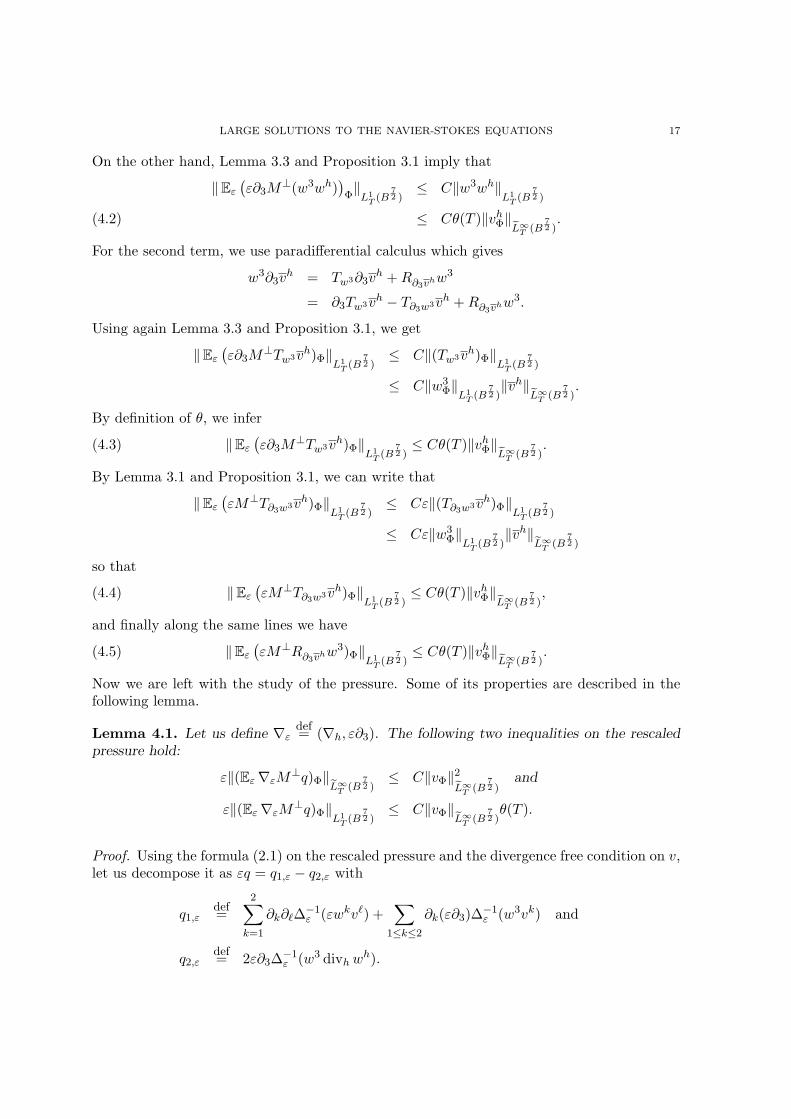
LARGE SOLUTIONS TO THE NAVIER-STOKES EQUATIONS 17
On the other hand, Lemma 3.3 and Proposition 3.1 imply that
‖Eε(ε∂3M
⊥(w3wh))
Φ‖L1
T (B72 )≤ C‖w3wh‖
L1T (B
72 )
≤ Cθ(T )‖vhΦ‖eL∞T (B72 ).(4.2)
For the second term, we use paradifferential calculus which gives
w3∂3vh = Tw3∂3v
h +R∂3vhw3
= ∂3Tw3vh − T∂3w3vh +R∂3vhw3.
Using again Lemma 3.3 and Proposition 3.1, we get
‖Eε(ε∂3M
⊥Tw3vh)Φ‖L1
T (B72 )≤ C‖(Tw3vh)Φ‖
L1T (B
72 )
≤ C‖w3Φ‖L1
T (B72 )‖vh‖eL∞T (B
72 ).
By definition of θ, we infer
(4.3) ‖Eε(ε∂3M
⊥Tw3vh)Φ‖L1
T (B72 )≤ Cθ(T )‖vhΦ‖eL∞T (B
72 ).
By Lemma 3.1 and Proposition 3.1, we can write that
‖Eε(εM⊥T∂3w3vh)Φ‖
L1T (B
72 )≤ Cε‖(T∂3w3vh)Φ‖
L1T (B
72 )
≤ Cε‖w3Φ‖L1
T (B72 )‖vh‖eL∞T (B
72 )
so that
(4.4) ‖Eε(εM⊥T∂3w3vh)Φ‖
L1T (B
72 )≤ Cθ(T )‖vhΦ‖eL∞T (B
72 ),
and finally along the same lines we have
(4.5) ‖Eε(εM⊥R∂3vhw3)Φ‖
L1T (B
72 )≤ Cθ(T )‖vhΦ‖eL∞T (B
72 ).
Now we are left with the study of the pressure. Some of its properties are described in thefollowing lemma.
Lemma 4.1. Let us define ∇εdef= (∇h, ε∂3). The following two inequalities on the rescaled
pressure hold:
ε‖(Eε∇εM⊥q)Φ‖eL∞T (B72 )≤ C‖vΦ‖2eL∞T (B
72 )
and
ε‖(Eε∇εM⊥q)Φ‖L1
T (B72 )≤ C‖vΦ‖eL∞T (B
72 )θ(T ).
Proof. Using the formula (2.1) on the rescaled pressure and the divergence free condition on v,let us decompose it as εq = q1,ε − q2,ε with
q1,εdef=
2∑k=1
∂k∂`∆−1ε (εwkv`) +
∑1≤k≤2
∂k(ε∂3)∆−1ε (w3vk) and
q2,εdef= 2ε∂3∆−1
ε (w3 divhwh).
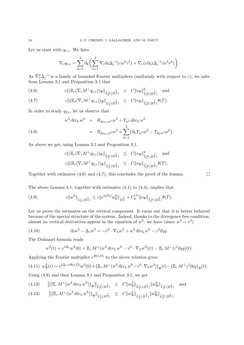
18 J.-Y. CHEMIN, I. GALLAGHER, AND M. PAICU
Let us start with q1,ε. We have
∇εq1,ε =2∑
k=1
∂k
( 2∑`=1
∇ε∂`∆−1ε (εwkv`) +∇ε(ε∂3)∆−1
ε (w3vk)).
As ∇2ε∆−1ε is a family of bounded Fourier multipliers (uniformly with respect to ε), we infer
from Lemma 3.1 and Proposition 3.1 that
ε‖(Eε(∇εM⊥q1,ε))Φ‖eL∞T (B72 )≤ C‖vΦ‖2eL∞T (B
72 )
and(4.6)
ε‖(Eε(∇εM⊥q1,ε))Φ‖L1
T (B72 )≤ C‖vΦ‖eL∞T (B
72 )θ(T ).(4.7)
In order to study q2,ε, let us observe that
w3 divhwh = Rdivh whw3 + Tw3 divhwh
= Rdivh whw3 +2∑
k=1
(∂kTw3wk − T∂kw3wk
).(4.8)
As above we get, using Lemma 3.1 and Proposition 3.1,
ε‖(Eε(∇εM⊥q2,ε))Φ‖eL∞T (B72 )≤ C‖vΦ‖2eL∞T (B
72 )
and
ε‖(Eε(∇εM⊥q2,ε))Φ‖L1
T (B72 )≤ C‖vΦ‖eL∞T (B
72 )θ(T ).
Together with estimates (4.6) and (4.7), this concludes the proof of the lemma.
The above Lemma 4.1, together with estimates (4.1) to (4.4), implies that
(4.9) ε‖wh‖L1
T (B72 )≤ ε‖ea|D3|wh0‖B 7
2+ C
(1)0 ‖vΦ‖eL∞T (B
72 )θ(T ).
Let us prove the estimates on the vertical component. It turns out that it is better behavedbecause of the special structure of the system. Indeed, thanks to the divergence free condition,almost no vertical derivatives appear in the equation of w3: we have (since w3 = v3)
Applying the Fourier multiplier eΦ(t,D) to the above relation gives
(4.11) w3Φ(t) = et∆ε+Φ(t,D)w3(0)+
(EεM⊥(w3 divhwh−vh ·∇hw3)
)Φ
(t)−(EεM⊥ε2∂3q
)Φ
(t).
Using (4.8) and then Lemma 3.1 and Proposition 3.1, we get∥∥(EεM⊥(w3 divhwh))
Φ
∥∥eL∞T (B72 )≤ C‖w3
Φ‖eL∞T (B72 )‖whΦ‖eL∞T (B
72 )
and(4.12) ∥∥(EεM⊥(w3 divhwh))
Φ‖L1
T (B72 )≤ C‖w3
Φ‖L1T (B
72 )‖whΦ‖eL∞T (B
72 ).(4.13)
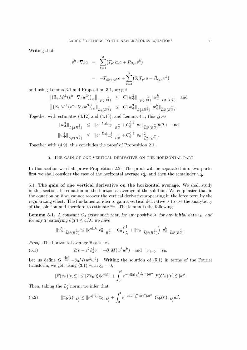
LARGE SOLUTIONS TO THE NAVIER-STOKES EQUATIONS 19
Writing that
vh · ∇ha =2∑
k=1
(Tvk∂ka+R∂kav
k)
= −Tdivh wha+2∑
k=1
(∂kTvka+R∂kav
k)
and using Lemma 3.1 and Proposition 3.1, we get∥∥(EεM⊥(vh · ∇hw3))
Φ
∥∥eL∞T (B72 )≤ C‖w3
Φ‖eL∞T (B72 )‖whΦ‖eL∞T (B
72 )
and∥∥(EεM⊥(vh · ∇hw3))
Φ‖L1
T (B72 )≤ C‖w3
Φ‖L1T (B
72 )‖whΦ‖eL∞T (B
72 ).
Together with estimates (4.12) and (4.13), and Lemma 4.1, this gives
‖w3Φ‖L1
T (B72 )≤ ‖ea|D3|w3
0‖B 72
+ C(1)0 ‖vΦ‖eL∞T (B
72 )θ(T ) and
‖w3Φ‖eL∞T (B
72 )≤ ‖ea|D3|w3
0‖B 72
+ C(1)0 ‖vΦ‖2eL∞T (B
72 ).
Together with (4.9), this concludes the proof of Proposition 2.1.
5. The gain of one vertical derivative on the horizontal part
In this section we shall prove Proposition 2.2. The proof will be separated into two parts:first we shall consider the case of the horizontal average vhΦ, and then the remainder whΦ.
5.1. The gain of one vertical derivative on the horizontal average. We shall studyin this section the equation on the horizontal average of the solution. We emphasize that inthe equation on v we cannot recover the vertical derivative appearing in the force term by theregularizing effect. The fundamental idea to gain a vertical derivative is to use the analyticityof the solution and therefore to estimate vΦ. The lemma is the following.
Lemma 5.1. A constant C0 exists such that, for any positive λ, for any initial data v0, andfor any T satisfying θ(T ) ≤ a/λ, we have
‖vhΦ‖eL∞T (B72 )≤ ‖ea|D3|vh0‖B 7
2+ C0
( 1λ
+ ‖vΦ‖eL∞T (B72 )
)‖vhΦ‖eL∞T (B
72 ).
Proof. The horizontal average v satisfies
(5.1) ∂tv − ε2∂23v = −∂3M(w3wh) and v|t=0 = v0.
Let us define Gdef= −∂3M(w3wk). Writing the solution of (5.1) in terms of the Fourier
transform, we get, using (3.1) with ξh = 0,
|F(vΦ)(t, ξ)| ≤ |Fv0(ξ)|ea|ξ3| +∫ t
0e−λ|ξ3|
R tt′ θ(t
′′)dt′′ |F(GΦ)(t′, ξ)|dt′.
Then, taking the L2j norm, we infer that
(5.2) ‖vΦ(t)‖L2j≤ ‖ea|D3|v0‖L2
j+∫ t
0e−cλ2j
R tt′ θ(t
′′)dt′′‖GΦ(t′)‖L2jdt′.
20 J.-Y. CHEMIN, I. GALLAGHER, AND M. PAICU
Now, let us estimate ‖GΦ(t′)‖L2j. For any function a, using the fact that the vector field w is
divergence free, let us write that
∂3(w3a) = ∂3
(Tw3a+Raw
3)
= ∂3Tw3a+R∂3aw3 −Ra divhwh
= ∂3Tw3a+R∂3aw3 −
2∑`=1
∂`Raw` +
2∑`=1
R∂`aw`.(5.3)
Thus, we infer that
G = −∂3MTw3wk −M(R∂3wkw3 +
2∑`=1
R∂`wkw` −2∑`=1
∂`Rw3w`)
= −∂3MTw3wk −M(R∂3wkw3 +
2∑`=1
R∂`wkw`).(5.4)
Now, let us study FM(Tab)Φ and FM(Rab)Φ for two functions a and b which have 0 horizontalaverage. As the two terms are identical, let us study the first one. By definition, we have
F(Tab)(t, (0, ξ3)) =
∑j
∫2jC∩B((0,ξ3),2j )
a((0, ξ3)− η)b(η)dη.
As θ(T ) ≤ λ−1a, by definition of Φ we have, for any η ∈ (Z2 \0)× R,
Then using (5.3) we get, thanks to Leibnitz formula,
M⊥∂3(w3vk) = M⊥∂3Tw3vk + F k with
F kdef= M⊥
(R∂3vkw3 −
2∑`=1
(∂`Rvkw` −R∂`vk
w`)).
Thanks to Lemma 3.1 and Proposition 3.1, we get
‖(EεM⊥F k)Φ‖eL∞T (B72 )≤ ‖(F k)Φ‖eL∞T (B
72 )
≤ C‖vΦ‖eL∞T (B72 )‖vhΦ‖eL∞T (B
72 ).
Together with Lemma 3.2, this gives
(5.7)∥∥(EεM⊥∂3(w3vh)
)Φ
∥∥eL∞T (B72 )≤ C0
( 1λ
+ ‖vΦ‖eL∞T (B72 )
)‖vhΦ‖eL∞T (B
72 ).
Now let us study the pressure term. Formula (2.1) together with the divergence free conditionleads to the decomposition q = qh(wh) + q3(v) with
qh(wh) def= ∆−1ε
((divhwh)2 +
∑1≤k,`≤2
∂kw`∂`w
k)
and(5.8)
q3(v) def= ∆−1ε
( ∑1≤`≤2
∂3v`∂`w
3).(5.9)
For the first term we use Bony’s decomposition in order to obtain
∂kw`∂`w
k = T∂kw`∂`wk +R∂`wk∂kw
`.
Then the Leibnitz formula implies that
(5.10) ∂kw`∂`w
k = ∂`T∂kw`wk + ∂kR∂`wkw` − T∂`∂kw`wk −R∂k∂`wkw`.
22 J.-Y. CHEMIN, I. GALLAGHER, AND M. PAICU
On the other hand, again by paradifferential calculus, we can write that
(divhwh)2 = Tdivh wh divhwh +Rdivh wh divhwh
= divh(Tdivh whwh +Rdivh whwh
)−
2∑k=1
(T∂k divh whwk +R∂k divh whwk
).(5.11)
Then Lemma 3.1 implies that
‖(Eε∇hqh(wh))Φ‖eL∞T (B72 )≤ C0‖(M⊥qh(wh))Φ‖eL∞(B
72 ).
Using Proposition 3.1 and the fact that the operators ∇h∆−1ε M⊥ and ∆−1
ε M⊥ are bounded(uniformly in ε) Fourier multipliers, we obtain
(5.12)∥∥(Eε(∇hqh(wh))
)Φ
∥∥eL∞T (B72 )≤ C0‖vhΦ‖2eL∞T (B
72 ).
For the second term, let us decompose q3(v) in the following way:
∂3v`∂`w
3 = T∂3v`∂`w3 +R∂`w3∂3v
`
= ∂`T∂3v`w3 + ∂3R∂`w3v` − T∂3∂`v`w3 −R∂3∂`w3v`.
Using now Lemma 3.1 together with Proposition 3.1 and Lemma 3.2, we obtain
(5.13)∥∥(Eε(∇hq3(v))
)Φ
∥∥eL∞T (B72 )≤ C0
( 1λ
+ ‖vΦ‖eL∞T (B72 )
)‖vh‖eL∞T (B
72 ).
The expected result is obtained putting together estimates (5.12) and (5.13) on the pressurewith estimates (5.6) and (5.7) on the nonlinear terms.
References
[1] M. Cannone, Y. Meyer and F. Planchon, Solutions autosimilaires des equations de Navier-Stokes,
Seminaire ”Equations aux Derivees Partielles” de l’Ecole polytechnique, Expose VIII, 1993–1994.[2] J.-Y. Chemin, Le systeme de Navier-Stokes incompressible soixante dix ans apres Jean Leray, Seminaire
et Congres, 9, 2004, pages 99–123.[3] J.-Y. Chemin, B. Desjardins, I. Gallagher and E. Grenier, Fluids with anisotropic viscosity, Modelisation
Mathematique et Analyse Numerique, 34, 2000, pages 315–335.[4] J.-Y. Chemin and I. Gallagher, On the global wellposedness of the 3-D Navier-Stokes equations with large
initial data, Annales de l’Ecole Normale Superieure, 39, 2006, pages 679–698.[5] J.-Y. Chemin and I. Gallagher, Wellposedness and stability results for the Navier-Stokes equations in R3
to appear in Annales de l’Institut Henri Poincare, Analyse Non Lineaire.[6] J.-Y. Chemin and I. Gallagher, Large, global solutions to the Navier-Stokes equations, slowly varying in
one direction, to appear in Transactions of the Americal Mathematical Society.[7] J.-Y. Chemin and N. Lerner, Flot de champs de vecteurs non-lipschitziens et equations de Navier-Stokes,
Journal of Differential Equations, 121, 1995, pages 314–328.[8] J.-Y. Chemin and P. Zhang, On the global wellposedness of the 3-D incompressible anisotropic Navier-
Stokes equations, Communications in Mathematical Physics, 272, 2007, pages 529–566.[9] L. Escauriaza, G. Seregin and V. Sverak, On the L3,∞ solutions to the Navier- Stokes equations and
backward uniqueness, Russ. Math. Surv., 58, 2003, pages 211–250.[10] H. Fujita and T. Kato, On the Navier-Stokes initial value problem I, Archive for Rational Mechanics and
Analysis, 16, 1964, pages 269–315.[11] I. Gallagher, D. Iftimie and F. Planchon, Asymptotics and stability for global solutions to the Navier–
Stokes equations, Annales de l’Institut Fourier, 53, 2003, pages 1387–1424.[12] I. Gallagher and M. Paicu, Remarks on the blow-up of solutions to a toy model for the Navier-Stokes
equations, submitted.
LARGE SOLUTIONS TO THE NAVIER-STOKES EQUATIONS 23
[13] Y. Giga and T. Miyakawa, Solutions in Lr of the Navier-Stokes initial value problem, Archiv for RationalMechanics and Analysis, 89, 1985, pages 267–281.
[14] D. Iftimie, A uniqueness result for the Navier-Stokes equations with vanishing vertical viscosity, SIAMJournal of Mathematical Analysis, 33, 2002), pages 1483–1493.
[15] D. Iftimie, G. Raugel and G.R. Sell, Navier-Stokes equations in thin 3D domains with Navier boundaryconditions, Indiana University Mathematical Journal, 56, 2007, pages 1083–1156.
[16] T. Kato, Strong Lp-solutions of the Navier-Stokes equation in Rm with applications to weak solutions,Mathematische Zeitschrift, 187, 1984, pages 471-480 .
[17] H. Koch and D. Tataru, Well–posedness for the Navier–Stokes equations, Advances in Mathematics, 157,2001, pages 22–35.
[18] O. Ladyzhenskaya, The mathematical theory of viscous incompressible flow. Second English edition, revisedand enlarged. T Mathematics and its Applications, Vol. 2 Gordon and Breach, Science Publishers, NewYork-London-Paris 1969 xviii+224 pp.
[19] S. Leibovich, A. Mahalov, E. Titi, Invariant helical subspaces for the Navier-Stokes equations. Archiv forRational Mechanics and Analysis, 112, 1990, pages 193–222.
[20] P.-G. Lemarie-Rieusset, Recent developments in the Navier-Stokes problem. Chapman and Hall/CRCResearch Notes in Mathematics, 43, 2002.
[21] J. Leray, Essai sur le mouvement d’un liquide visqueux emplissant l’espace, Acta Matematica, 63, 1933,pages 193–248.
[22] J. Leray, Etude de diverses equations integrales non lineaires et de quelques problemes que posel’hydrodynamique. Journal de Mathematiques Pures et Appliquees, 12, 1933, pages 1–82.
[23] A. Mahalov and B. Nicolaenko, Global solvability of three-dimensional Navier-Stokes equations with uni-formly high initial vorticity, (Russian. Russian summary) Uspekhi Mat. Nauk 58, 2003, pages 79–110;translation in Russian Math. Surveys 58, 2003, pages 287–318.
[24] Y. Meyer, Wavelets, Paraproducts and Navier–Stokes. Current Developments in Mathematics, Interna-tional Press, Cambridge, Massachussets, 1996.
[25] S. Montgomery-Smith, Finite-time blow up for a Navier-Stokes like equation, Proc. Amer. Math. Soc. 129,2001, pages 3025–3029.
[26] J. Necas, M. Ruzicka and V. Sverak, On Leray’s self-similar solutions of the Navier-Stokes equations, ActaMathematica, 176, 1996, pages 283–294.
[27] M.Paicu, Equation anisotrope de Navier-Stokes dans des espaces critiques, Revista Rev. MatemticaIberoamericana, 21, 2005, page 179–235.
[28] G. Ponce, R. Racke, T. Sideris and E. Titi, Global stability of large solutions to the 3D Navier-Stokesequations, Communications in Mathematical Physics, 159, 1994, pages 329–341.
[29] G. Raugel and G.R. Sell, Navier-Stokes equations on thin 3D domains. I. Global attractors and globalregularity of solutions, Journal of the American Mathematical Society, 6, 1993, pages 503–568.
[30] M. Sammartino and R. E. Caflisch, Zero Viscosity Limit for Analytic Solutions, of the Navier-StokesEquation on a Half-Space. I. Existence for Euler and Prandtl Equations, Communications in MathematicalPhysics, 192, 1998, pages 433–461.
[31] M. Ukhovskii and V. Iudovich, Axially symmetric flows of ideal and viscous fluids filling the whole space.Prikl. Mat. Meh. 32 59–69 (Russian); translated as Journal of Applied Mathematics and Mechanics, 32,1968, pages 52–61.
[32] F. Weissler, The Navier-Stokes Initial Value Problem in Lp, Archiv for Rational Mechanics and Analysis,74, 1980, pages 219-230.
24 J.-Y. CHEMIN, I. GALLAGHER, AND M. PAICU
(J.-Y. Chemin) Laboratoire J.-L. Lions UMR 7598, Universite Pierre et Marie Curie, 175, rue duChevaleret, 75013 Paris, FRANCE


![CHAPTER 5 THE ALLARD REGULARITY THEOREMmaths-proceedings.anu.edu.au/.../CMAProcVol3-Chapter5.pdfCHAPTER 5 THE ALLARD REGULARITY THEOREM Here we discuss Allard's ([AWl]) regularity](https://static.documents.pub/doc/80x56/5fb2cc5e95482068621741eb/chapter-5-the-allard-regularity-theoremmaths-chapter-5-the-allard-regularity-theorem.jpg)


![T2 · 2019. 8. 1. · 310 M.N. MUKHERJEE AND S.P. SINHA regularity were also defined in [6]. Wecharacterize fuzzy regularity and these weaker forms of fuzzy regularity in terms of](https://static.documents.pub/doc/80x56/60b0546db5896d7af80bbfee/t2-2019-8-1-310-mn-mukherjee-and-sp-sinha-regularity-were-also-defined.jpg)


