Institute of Physical Geography, University of Frankfurt, Frankfurt am Main, Germany
Received: 24 October 2007 – Published in Hydrol. Earth Syst. Sci. Discuss.: 15 November 2007Revised: 10 March 2008 – Accepted: 23 March 2008 – Published: 29 May 2008
Abstract. Long-term average groundwater recharge, whichis equivalent to renewable groundwater resources, is the ma-jor limiting factor for the sustainable use of groundwater.Compared to surface water resources, groundwater resourcesare more protected from pollution, and their use is less re-stricted by seasonal and inter-annual flow variations. To sup-port water management in a globalized world, it is necessaryto estimate groundwater recharge at the global scale. Here,we present a best estimate of global-scale long-term aver-age diffuse groundwater recharge (i.e. renewable ground-water resources) that has been calculated by the most recentversion of the WaterGAP Global Hydrology Model WGHM(spatial resolution of 0.5◦ by 0.5◦, daily time steps). Theestimate was obtained using two state-of-the-art global datasets of gridded observed precipitation that we corrected formeasurement errors, which also allowed to quantify the un-certainty due to these equally uncertain data sets. The stan-dard WGHM groundwater recharge algorithm was modifiedfor semi-arid and arid regions, based on independent esti-mates of diffuse groundwater recharge, which lead to anunbiased estimation of groundwater recharge in these re-gions. WGHM was tuned against observed long-term av-erage river discharge at 1235 gauging stations by adjusting,individually for each basin, the partitioning of precipitationinto evapotranspiration and total runoff. We estimate thatglobal groundwater recharge was 12 666 km3/yr for the cli-mate normal 1961–1990, i.e. 32% of total renewable wa-ter resources. In semi-arid and arid regions, mountainousregions, permafrost regions and in the Asian Monsoon re-gion, groundwater recharge accounts for a lower fractionof total runoff, which makes these regions particularly vul-nerable to seasonal and inter-annual precipitation variabilityand water pollution. Average per-capita renewable ground-
water resources of countries vary between 8 m3/(capita yr)for Egypt to more than 1 million m3/(capita yr) for the Falk-land Islands, the global average in the year 2000 being2091 m3/(capita yr). Regarding the uncertainty of estimatedgroundwater resources due to the two precipitation data sets,deviation from the mean is 1.1% for the global value, and lessthan 1% for 50 out of the 165 countries considered, between1 and 5% for 62, between 5 and 20% for 43 and between 20and 80% for 10 countries. Deviations at the grid scale can bemuch larger, ranging between 0 and 186 mm/yr.
1 Introduction
Groundwater recharge is the major limiting factor for the sus-tainable use of groundwater because the maximum amountof groundwater that may be withdrawn from an aquifer with-out irreversibly depleting it, under current climatic condi-tions, is approximately equal to long-term (e.g. 30 years) av-erage groundwater recharge. Therefore, long-term averagegroundwater recharge is equivalent to renewable groundwa-ter resources. Depletion of non-renewable (“fossil”) ground-water resources by human water withdrawals can be quanti-fied by comparing withdrawal rates to groundwater recharge.Groundwater recharge either occurs, locally, from surfacewater bodies or, in diffuse form, from precipitation via theunsaturated soil zone. Long-term average diffuse groundwa-ter recharge is the part of precipitation that does not evap-otranspirate and does not run off to a surface water bodyon the soil surface or within the unsaturated zone. Onlydiffuse groundwater recharge is taken into account in thispaper, as groundwater recharge from surface water bodiescannot be estimated at the macro-scale. In semi-arid andarid regions, outside the mountainous headwater regions,neglecting groundwater recharge from surface-water bodiesmay lead to a significant underestimation of total renewable
Published by Copernicus Publications on behalf of the European Geosciences Union.
864 P. Doll and K. Fiedler: Global-scale modeling of groundwater recharge
groundwater resources. Hereafter, the term groundwaterrecharge refers only to diffuse recharge.
In most regions of the world, a large part of groundwaterrecharge is transported to surface waters, and is thus includedin estimates of surface water resources derived from river dis-charge measurements (groundwater close to the coast maydischarge directly into the ocean, and in semi-arid and aridregions, a part of the groundwater recharge evapotranspi-rates before discharging into a river). Nevertheless, it is use-ful to quantify groundwater resources separately. First, theyare much better protected from pollution than surface wa-ter resources. Second, the use of groundwater resources ismuch less restricted by seasonal or inter-annual flow vari-ations (e.g. drought periods) than the use of surface water.To support water management in a globalized world, it istherefore necessary to estimate, in a spatially resolved way,groundwater recharge and thus renewable groundwater re-sources at the global scale.
Different from surface water resources, groundwaterrecharge cannot be easily measured. While surface wa-ter resources are concentrated in the river channels of adrainage basin and thus can be determined by measuringriver discharge, groundwater recharge, like precipitation, isdistributed spatially, and a very large number of measure-ments would be necessary to obtain a good estimate for asizeable area. Besides, groundwater recharge, unlike precip-itation, cannot be directly measured as a volume flow butmust be determined by a variety of indirect methods whereeither the unsaturated zone or the groundwater is analyzed(Lerner, 1990; Simmers, 1997; Scanlon et al., 2002). Inhumid regions, groundwater recharge is generally estimatedfrom the baseflow component of measured river discharge.However, it is well known that computed baseflow valuesstrongly depend on the method that has been applied forbaseflow analysis such that baseflow indices (baseflow as afraction of total flow) can vary by a factor of 2 (Tallaksen,1995; Bullock et al., 1997; Neumann, 2005). Besides, base-flow analysis does not lead to meaningful results if gaugingstations are downstream of large reservoirs, lakes or wetlands(L’vovich, 1979). Baseflow analysis in semi-arid and arid re-gions is likely to lead to an underestimation of groundwa-ter recharge, as part of the recharge evapotranspirates beforereaching (larger) rivers (Margat, 1990:33). Finally, it mustbe kept in mind that the concept of renewable groundwaterresources and its relation to groundwater recharge and base-flow is scale-dependent as a part of the groundwater rechargemight reappear as surface water after a very short travel dis-tance.
The first global-scale study of groundwater recharge wasaccomplished by L’vovich (1979), whose global map ofgroundwater recharge was based on the estimation of thebaseflow component of observed river discharge. A numberof institutions have compiled global lists of country valuesof groundwater recharge (Margat, 1990; WRI, 2000; FAO,2003, 2005). In the compilation of WRI (2000), many val-
ues stem from Margat (1990) which again often used esti-mates of the global analysis of L’vovich (1979). The mostrecent estimates of groundwater recharge per country havebeen compiled by FAO (2005), and include mainly data col-lected for FAO country reports (150 countries) and data fromnational sources, but a few country values are still thoseof the global-scale analysis of L’vovich (1979). The coun-try values of groundwater recharge have been obtained byvery diverse methods mostly in the 70s, 80s and 90s of the20th century. WRI (2005a, b), in their presentation of theFAO (2005) groundwater recharge values, warn that “all datashould be considered order-of-magnitude estimates” and that“cross-country comparisons should therefore be made withcaution”. Comparing WRI (2000) and FAO (2005) estimates,for the 131 countries for which values exist in both data sets,69 country values are the same, while 14 country values dif-fer by more than 50%.
After L’vovich (1979), no other global-scale analysis wasperformed until Doll et al. (2002) obtained the first model-based estimates of groundwater recharge at the global scale.With a spatial resolution of 0.5◦ geographical latitude by0.5◦ geographical longitude, diffuse groundwater rechargefor the climate normal 1961–1990 was estimated with theglobal hydrological model WGHM (WaterGAP Global Hy-drology Model, Doll et al., 2003; Alcamo et al., 2003). Inthat version of WGHM, long-term average total runoff, i.e.the sum of groundwater recharge and fast surface and sub-surface flow, was tuned against observed river discharge at724 stations world-wide by adjusting basin-specific parame-ters. Later, the WGHM groundwater recharge algorithm wasimproved for semi-arid and arid regions, and the model wasused to estimate the impact of climate change on groundwa-ter recharge (Doll and Florke, 2005). The model was alsoapplied to analyze the contribution of groundwater to large-scale water storage variations as derived from gravity mea-surements of the GRACE satellite mission (Guntner et al.,2007a, b). The analysis showed a large spatial variabilityof groundwater storage dynamics, both in absolute valuesand as a fraction of total water storage. As expected, be-cause of its longer residence times, groundwater can decreasethe seasonal variation of total water storage, and it tends tohave a larger contribution to total storage change for inter-annual than for seasonal storage dynamics. Besides, WGHMgroundwater recharge estimates were included in the Hydro-geological Map of Africa of Seguin (2005).
The goal of this paper is to present the most recent es-timates of groundwater recharge at the global scale as ob-tained with the new WGHM version 2.1f for the time period1961–1990. This new model version differs from the formerversions by, among other changes, an increased number ofnow 1,235 river discharge observation stations that are usedto tune the model. These stations lead to an improved spatialrepresentation of total runoff (Hunger and Doll, 2008), andthus probably groundwater recharge. Besides, two state-of-the-art precipitation data sets are used as alternative model
P. Doll and K. Fiedler: Global-scale modeling of groundwater recharge 865
Fig. 1. Schematic representation of water flows and storages in each 0.5 degree grid cell as simulated by the global hydrological modelWGHM, highlighting the computation of diffuse groundwater recharge.Epot: potential evapotranspiration,Eact: actual evapotranspirationfrom soil.
inputs, in order to characterize the important uncertainty ofestimated groundwater recharge that is due to uncertainty ofglobal-scale precipitation estimates. Precipitation is the ma-jor driver of groundwater recharge; for areas with arid to hu-mid climate in southwestern USA, Keese et al. (2005) foundthe mean annual precipitation explains 80% of the variationof groundwater recharge. WGHM groundwater recharge es-timates will be included in the Global Map of Groundwa-ter Resources developed in UNESCO’s “World-wide Hydro-geological Mapping and Assessment Program” WHYMAP(http://www.whymap.org, final release summer 2008).
Other hydrological models as well as the land surfaceschemes of climate models also compute variables that couldbe considered as diffuse groundwater recharge. To ourknowledge, however, these model outputs have not yet beenanalyzed and interpreted at the global scale. In the SecondGlobal Soil Wetness Project, for example, where the out-put of 13 land surface models was compared, groundwaterrecharge was lumped with interflow (Dirmeyer et al., 2005).
In the next section, we present the WGHM approach ofmodeling groundwater recharge as well as the precipitationdata sets. In Sect. 3, we show the computed global ground-water recharge and resources maps including a quantifica-tion of the error due to precipitation uncertainty and comparegroundwater resources to total water resources. In Sect. 4, wediscuss the quality of the results, while in Sect. 5, we drawsome conclusions.
2 Methods and data
2.1 Model description
A detailed presentation of the WaterGAP Global Hydrol-ogy Model (WGHM), including process formulations, in-put data, model tuning, and validation is given by Doll etal. (2003). The newest model version WGHM 2.1f is pre-sented by Hunger and Doll (2008). Here, a short modeloverview is provided, and the groundwater recharge algo-rithm is described in detail.
2.1.1 WGHM overview
The WaterGAP 2 model (Alcamo et al., 2003) includes boththe global hydrological model WGHM and a number of wa-ter use models that compute consumptive and withdrawalwater use for irrigation (Doll and Siebert, 2002), livestock,industry (Vassolo and Doll, 2006) and households. There-fore, in WGHM, river discharge reduction due to human wa-ter use can be taken into account by subtracting consumptivewater use (water withdrawals minus return flows) from sur-face water bodies. It is assumed that total consumptive wateruse is taken from surface waters (Fig. 1) as there is currentlyno information, at the global scale, on the fraction of totalwater withdrawal that is abstracted from groundwater.
WHGM simulates the vertical water balance and lateraltransport with a spatial resolution of 0.5◦ by 0.5◦, coveringthe global land area with the exception of Antarctica (66 896
Fig. 2. Location of 1235 river discharge stations for basin-specific tuning, location of independent estimates of groundwater recharge, andsemi-arid and arid areas where modified groundwater recharge algorithm was applied.
cells). Figure 1 shows the storages and fluxes that are sim-ulated for each grid cell with a time step of 1 day. It is as-sumed that groundwater recharged within one cell leaves thegroundwater store as baseflow within the same cell. Waterflow between grid cells is assumed to occur only as riverdischarge, following a global drainage direction map (Dolland Lehner, 2002). Water flow from surface water bodies togroundwater is not taken into account. For each time step,the net runoff of each cell is computed as the balance of pre-cipitation, evapotranspiration from canopy, soil and surfacewaters, and water storages changes within the cell.
WGHM is tuned, individually for 1235 large drainagebasins, against observed long-term average river discharge(Fig. 2) by optimizing a parameter in the soil water balancealgorithm, the so-called runoff coefficient, and, if necessary,by introducing correction factors (Hunger and Doll, 2008).By tuning, the difference between long-term average precip-itation and evapotranspiration, i.e. total runoff, in each tun-ing basin (during the observation period) becomes equal tolong-term average observed river discharge. Given the largeuncertainties of both the climate input data (in particularprecipitation) and the hydrological model, this type of tun-ing helps to obtain rather realistic water flows in the basins.However, in semi-arid and arid regions, tuning is likely tolead to an underestimation of runoff generation, as river dis-charge at a downstream location is likely to be less than therunoff generated in the basin, due to evapotranspiration ofrunoff and leakage from the river. The tuning basins coveralmost half of the global land area (except Antarctica andGreenland). For the remaining river basins, the runoff coef-ficients are obtained by regionalizing the runoff coefficientsof the tuning basins. This was done by a multiple regressionanalysis which relates the runoff coefficient for all the gridcells within the basin to the following basin characteristics:
long-term average temperature, fraction of open water sur-faces and length of non-perennial rivers (Doll et al., 2003).Outside the tuning basins, the correction factors are set to 1.
2.1.2 Groundwater recharge algorithm
Daily groundwater rechargeRg is computed as part of thevertical water balance of each grid cell (Fig. 1). In order tocalculateRg, total runoff from landRl is partitioned into fastsurface and subsurface runoffRs and groundwater rechargeRg. Following a heuristic approach, this is done based onqualitative knowledge about the influence of the followingcharacteristics on the partitioning of runoff: relief, soil tex-ture, hydrogeology and the occurrence of permafrost andglaciers. With steeper slopes, finer soil textures and less per-meable aquifers, groundwater recharge as a fraction of totalrunoff from land is expected to decrease, and permafrost andglaciers are assumed to prevent groundwater recharge. Be-sides, soils have a texture-related infiltration capacity, which,if exceeded in case of intense rainfalls, prevents groundwaterrecharge (causing surface runoff to occur); the finer the soiltexture, the lower the infiltration capacity. Accordingly,Rg
is computed as
Rg = min(Rg max, fgRl) with fg = frftfhfpg (1)
Rg max = soil texture-specific maximum groundwaterrecharge (infiltration capacity) [mm/d]
Rl = total runoff of land area of cell [mm/d]fg = groundwater recharge factor (0≤fg<1)fr = relief-related factor (0<fr<1)ft = soil texture-related factor (0≤ft≤1)fh = hydrogeology-related factor (0<fh<1)fpg = permafrost/glacier-related factor (0≤fpg≤1)
P. Doll and K. Fiedler: Global-scale modeling of groundwater recharge 867
A number of other possible physio-geographic character-istics like land cover, precipitation, surface drainage densityand depth to groundwater have not been included in the al-gorithm for various reasons. Haberlandt et al. (2001) found,in their study on baseflow indices BFI (baseflow as a ratio oftotal runoff from land) in the Elbe basin that the proportionof forest and arable land (i.e. land cover) in sub-basins of orbelow the size of 0.5◦ grid cells only had a weak influence onBFI. Precipitation was not included as a predictor in Eq. (1)as 1) it is already included as an inflow to the model, and2) two regional-scale regression analyses of BFI lead to con-flictive results. In the Central European Elbe basin, wheremore rain falls in mountainous areas, there was a strong neg-ative correlation between BFI and precipitation (Haberlandtet al., 2001). The opposite behavior was found in SouthernAfrica where more rain falls in the northern flat regions (Bul-lock et al., 1997). Depth to groundwater and surface drainagedensity, which were identified by Jankiewicz et al. (2005) asgood predictors for estimating groundwater recharge in Ger-many at a spatial resolution 1 km by 1 km (in addition to totalrunoff, soil texture, slope, and land cover), are not availableat the global scale at all or not at an appropriate resolution, re-spectively. Besides, in the regression analysis of Jankiewiczet al. (2005), the depth to groundwater was found to have theopposite effect in areas with high (>200 mm/yr) vs. low totalrunoff.
Global-scale information on relief (G. Fischer, IIASA,personal communication, 1999), soil texture (FAO, 1995),hydrogeology (Canadian Geological Survey, 1995) and theoccurrence of permafrost and glaciers (Brown et al., 1998;Hoelzle and Haeberli, 1999) was available at different spatialresolutions and is described in more detail in Appendix A.The cell-specific values of all four basic factors and of thetexture specific maximum groundwater recharge in Eq. (1)were computed by first assigning values to the attributes ofthe global data sets (e.g. aft -value of 1 was assigned tocoarse, aft -value of 0.7 to fine soil texture, Appendix A2).Then, the values were upscaled to 0.5◦ by 0.5◦.The spe-cific values for the four factorsfr , ft , fh andfpg are ex-pert guesses that have been adjusted iteratively by comparingthe resulting spatial distribution of groundwater recharge andbase flow indices with the global map of L’vovich (1979) aswell as regional maps for the Elbe basin (Haberlandt et al.,2001), Southern Africa (Bullock et al., 1997) and Southwest-ern Germany (B. Lehner, personal communication).
For semi-arid and arid conditions, modeling of runoff andgroundwater recharge is generally found to be more diffi-cult than for humid areas, mainly due to the small valuesof these variables. Besides, river discharge measurementsare not as indicative of groundwater recharge as under humidconditions, where most of the groundwater recharge reachesa river. However, under semi-arid and arid conditions, it ispossible to estimate long-term average groundwater rechargebased on the analysis of chloride profiles in the soil and iso-tope measurements. Such estimates for 25 locations which
0.001
0.010
0.100
1.000
10.000
100.000
1000.000
0.001 0.010 0.100 1.000 10.000 100.000 1000.000
independent estimates of long-term average groundwater recharge [mm/yr]
mo
de
lle
dlo
ng
-te
rma
ve
rag
e(1
96
1-9
0)
gro
un
dw
ate
rre
ch
arg
e[m
m/y
r]
standard
modified
average value for 51 grid cells:
- with standard model algorithm: 16.9 mm/yr
- with modified model algorithm: 8.3 mm/yr
- independent estimates: 8.6 mm/yr
Fig. 3. Improved modeling of groundwater recharge due to mod-ified groundwater recharge algorithm for semi-arid regions: com-parison of independent estimates of long-term average groundwaterrecharge for 51 grid cells in semi-arid regions with modeled valuesas computed with the standard and the modified algorithm (usingGPCC precipitation).
are representative not only for the profile location but a largerarea of 25 km by 25 km were compiled by Mike Edmunds(University of Oxford, personal communication, 2003) andwere used to test the performance of Eq. (1), and to modifythe groundwater recharge algorithm of WGHM for semi-aridand arid grid cells (Fig. 2). In most cases, the data are rep-resentative for the 50–100 year period before the measure-ments. The observed data are from Northern and SouthernAfrica, the Near East, Asia and Australia (Fig. 2). In ad-dition, groundwater recharge as computed by a meso-scalehydrological model of the Death Valley region in southwest-ern USA (Hevesi et al., 2003) was taken into account. Themeso-scale model results, which are representative for thetime period 1950–1999, were upscaled to derive estimatesfor the 26 0.5◦ grid cells of WGHM which cover the region(Fig. 2).
We found that WGHM, with Eq. (1), significantly over-estimates groundwater recharge at the semi-arid and aridobservation sites, in particular groundwater recharge below20 mm/a (Fig. 3). This could be caused by either an overes-timation of total runoff (likely in semi-arid and arid basinswithout discharge measurements) or an overestimation ofgroundwater recharge as a fraction of total runoff. For theDeath Valley region, WGHM overestimates total runoff byabout an order of 10 (50 mm/yr instead of 5 mm/yr), whichcan only partially be explained by an overestimation of pre-cipitation. Where the groundwater recharge fraction is over-estimated, the preferred tuning method would be to modify
868 P. Doll and K. Fiedler: Global-scale modeling of groundwater recharge
the groundwater recharge factors in Eq. (1). However, ananalysis of the 51 grid cells with independent estimatesshowed that an adjustment of the recharge factors cannot leadto the necessary decrease in groundwater recharge, as mostcells that require a strong reduction of computed groundwa-ter recharge have low relief, coarse soil and young sedimen-tary aquifers, which means that they should have relativelylarge groundwater recharge fractions. We concluded that theWGHM conceptual model of groundwater recharge is lessappropriate for semi-arid than for humid regions, as, com-pared to humid regions, semi-arid and arid regions share thefollowing characteristics:
– A larger variability of precipitation with more heavyrainfalls
– Surface crusting in areas of weak vegetation cover,which strongly reduces infiltration into the soil
– Reduced infiltration of heavy rain into dry soil due topore air which has to be released first to allow the infil-tration. Additionally, the moistening of dry soil surfacesis reduced due to hydrophobic behavior of dried organicmaterials.
– More infiltration and thus groundwater recharge in soilswith fine texture as compared to soils with coarse tex-ture. In very dry conditions, the low unsaturated hy-draulic conductivity of sands, for example, leads to alower infiltration capacity for sand as compared to loam,which, at the same matric potential, has a much higherwater content and unsaturated hydraulic conductivity.
– In some regions, groundwater recharge only occurs viafissures in crystalline rock which allow the rainwater toleave the zone of capillary rise faster than in the case ofsand. Rainwater that remains in the capillary zone evap-orates due to high temperatures and radiation in semi-arid regions. In humid regions, groundwater recharge infissured crystalline rocks is expected to be lower than insandy sediments.
Altogether, in semi-arid regions groundwater recharge ap-pears to be confined to periods of exceptionally heavy rain-fall (Vogel and Van Urk, 1975), in particular if soil tex-ture is coarse (Small, 2005). Therefore, the computation ofgroundwater recharge in semi-arid and arid grid cells, witha medium to coarse soil texture, was modified such thatgroundwater recharge as modeled with Eq. (1) occurs onlyif the daily precipitation is larger than 10 mm/d. Followingthe definition of UNEP and the United Nations Conventionto Combat Desertification (UNEP, 1992), semi-arid/arid gridcells are those with long-term average (1961–1990) precip-itation less or equal to half the potential evapotranspiration.The grid cells which obey this rule but are north of 60◦Nwere not defined as “semi-arid”. This modification of the
groundwater recharge algorithm resulted in an unbiased esti-mation of groundwater recharge (Fig. 3) and also improvedthe correlation between observed and computed values (fromR2=0.14 toR2=0.37)
2.2 Precipitation data sets
WGHM is driven by time series of 0.5◦ gridded observedmonthly climate variables between 1901 and 2002, includ-ing precipitation, air temperature, cloudiness and number ofwet days (CRU TS 2.0 data set, Mitchell and Jones, 2005).Daily observed climate data are not available globally at the0.5◦ resolution for a period of 30 years, i.e. long enough toaverage out temporal climate variability. Daily values forlong periods of time can only be obtained from re-analysis,i.e. computations with general circulation models, but thecomputed precipitation fields do not capture the actual pre-cipitation patterns in a satisfactory manner. This results in aless satisfactory simulation of observed soil moisture dynam-ics when used as input into land surface models (Guo et al.,2006). Therefore, in this study, monthly observation-basedclimate data are scaled down to daily values. Downscalingprecipitation from monthly to daily values is based on thenumber of wet days per month, assuming the same grid-cellprecipitation on each wet day of a month, while daily tem-perature and cloudiness are obtained by cubic spline interpo-lation. For precipitation, the most important climatic driverof groundwater recharge, there is another 0.5◦ gridded globaldata set of long duration, the GPCC Full Data Product Ver-sion 3, for 1950–2004 (Fuchs et al., 2007). The two differentprecipitation data sets are based on different methods for thespatial interpolation of observation data. For the CRU dataset, 1961–1990 precipitation normals at 19 295 stations werecombined with time series at less stations of temporally vary-ing numbers to construct gridded time series from anomalies(New et al., 1999, 2000). For the GPCC data set, only thestation data available for the month of interest are taken intoaccount, thus losing information on spatial variability fromthe precipitation normals. For the period 1961–1990, pre-cipitation time series are available for about 15 000 stations(Fuchs et al., 2007). The differences between the two precip-itation data sets are large at the grid-scale (Fig. 4). For someparts of the world, e.g. the Himalayas, the long-term averageprecipitation values differ by more than a factor of two, andfor many parts of the world, by more than 20%. In the Hi-malayas, CRU precipitation seems to be shifted towards theNortheast as compared to GPCC. According to CRU, meanannual long-term average precipitation for 1961–1990 is 721mm/yr over the continents, as compared to 708 mm/yr ac-cording to GPCC. Differences are larger for individual years.It is not possible to judge which of the two data sets better re-flects actual precipitation. Therefore, both precipitation datasets are considered to be of equal reliability, and the best es-timate of groundwater recharge is assumed to be equal to themean of the groundwater recharge values obtained by using
P. Doll and K. Fiedler: Global-scale modeling of groundwater recharge 869
�������������������� ���
�� ��� ������
Fig. 4. Difference between the two available 0.5◦ global data sets of time series of gridded observed precipitation: ratio of CRU 1961-1990mean annual precipitation to GPCC 1961-1990 mean annual precipitation.
the two different precipitation data sets as input to WGHM.
None of the precipitation data sets is corrected for ob-servational errors, i.e. the typical wind-induced undercatchof especially solid precipitation. We developed the follow-ing equation to correct the time series of gridded observedmonthly precipitationPo, using catch ratios of Adam andLettenmaier (2003):
Pc = Po
[(1
CR− 1
)R(T )
R(Tmean)+ 1
](2)
Pc = corrected precipitation value [mm/month]CR = 0.5◦ gridded mean monthly catch ratio (mea-
sured precipitation as a ratio of actual precip-itation) for 1979–1998
R = snow as a fraction of total monthly precipita-tion (a function of monthly temperature)
T = temperature of specific monthTmean= average temperature 1961–1990
The mean monthly catch ratios were obtained by analyzingthe climatic conditions at 7898 climate stations between 1979and 1998, and by taking into account the different gaugetypes that are in use around the world (Adam and Letten-maier, 2003). In some areas, extremely high values ofCR inthe data of Adam and Lettenmaier (2003), which are likelydue to the interpolation algorithm, were smoothed. Particu-larly low catch ratios are observed in case of snow. In caseof precipitation time series, it is therefore important to cor-rect e.g. precipitation in January 1965 more than in January1966, if a larger fraction of precipitation fell as snow in Jan-uary 1965 than in 1966. This adjustment was done using theempirical functionR of Legates (1987) which relates snow
as a fraction of total monthly precipitation to monthly tem-peratureT , with
R =1
1 + 1.61(1.35)T(3)
Correction ofPo was limited to a range between 1 and 2.3.Correction byR(T )/R(Tmean) overestimates the impact of in-terannual variability of monthly temperatures on the neces-sary precipitation correction if catch ratios are not affectedby snow, i.e. at high temperatures. If this correction is onlyapplied at mean monthly temperatures below 3◦C, computedlong-term average groundwater recharge is not significantlychanged. The global value (ensemble mean using GPCCand CRU precipitation data) decreases by only 0.5%, andfor 83.3% and 99.77% of all grid cells, long-term averagegroundwater recharge changes by less than 1 and 5 mm/yr,respectively.
Correction of GPCC 1961–1990 precipitation according toEq. (2) increased the global mean by 11.6%, from 708 mm/yrto 790 mm/yr, with increases of annual precipitation rangingbetween a few percent and 30% in most areas of the globe.The relative changes of the CRU precipitation due to correc-tion are very similar. WGHM was tuned separately with eachof the two precipitation data sets.
3 Results
3.1 Groundwater recharge
The global map of long-term average diffuse groundwaterrecharge for the period 1961–1990 (Fig. 5a) presents the en-semble mean of two WGHM model runs with either GPCCor CRU precipitation data as input. The mean represents
870 P. Doll and K. Fiedler: Global-scale modeling of groundwater recharge
0 2 20 100 300 1000
0 1 3 10 30 200
a)
b)
Fig. 5. Long-term average diffuse groundwater recharge for the time period 1961–1990 in mm/yr; ensemble mean of groundwater rechargeas computed by two WGHM model runs with either GPCC or CRU precipitation data as input(a). Absolute difference between groundwaterrecharge computed with either one of the two precipitation data sets and the ensemble mean value, in mm/yr(b).
a best estimate because the quality of the two precipitationdata sets is judged to be equal. Both precipitation data setshave been corrected for observational errors by the samemethod. Grid-scale groundwater recharge ranges from 0 to960 mm/yr, with the highest values occurring in the humidtropics. Values over 300 mm/yr are also computed for someparts of northwestern Europe and the Alps. Europe is thecontinent with the smallest fraction of regions with ground-water recharge below 20 mm/yr. Such low values occur inthe dry subtropics and in Arctic regions (mainly due to per-mafrost).
Figure 5b shows the uncertainty of estimated groundwaterrecharge that is due to the use of two different precipitationdata sets. The absolute difference between GPCC (or CRU)groundwater recharge per grid cell and the ensemble mean
ranges between 0 and 186 mm/yr, and at the scale of the 0.5◦
grid cell, the percent differences can be quite high (compareFigs. 5a and b). The spatial pattern of uncertainty is due tothe combination of 1) the often very high differences betweenthe precipitation data sets (Fig. 4), and 2) the runoff coeffi-cients and correction factors, which are equal within eachriver basin and differ between the GPCC and CRU modelruns.
The differences between the results for the two precipi-tation data sets become, in general, smaller with increasingsize of the considered area, e.g. for countries (Appendix B)and continents (Table 1). For 50 out of the 165 countriesconsidered, the deviation from the mean was less than 1%,for 62 between 1 and 5%, for 43 between 5 and 20% andfor 10 between 20 and 80%. Deviations of more than 50%
P. Doll and K. Fiedler: Global-scale modeling of groundwater recharge 871
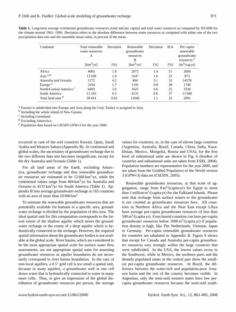
Table 1. Long-term average continental groundwater resources (total and per capita) and total water resources as computed by WGHM forthe climate normal 1961–1990. Deviation refers to the absolute difference between water resources as computed with either one of the twoprecipitation data sets and the ensemble mean value, in percent of the mean.
Continent Total renewable Deviation Renewable Deviation B/A Per capitawater resources groundwater renewable
a Eurasia is subdivided into Europe and Asia along the Ural; Turkey is assigned to Asia.b Including the whole island of New Guinea.c Including Greenland.d Excluding Antarctica.e Population data based on CIESIN GPWv3 for the year 2000.
occurred in case of the arid countries Kuwait, Qatar, SaudiArabia and Western Sahara (Appendix B). At continental andglobal scales, the uncertainty of groundwater recharge due tothe two different data sets becomes insignificant, except forthe dry Australia and Oceania (Table 1).
For all land areas of the Earth, excluding Antarc-tica, groundwater recharge and thus renewable groundwa-ter resources are estimated to be 12 666 km3/yr, while thecontinental values range from 404 km3/yr for Australia andOceania to 4131 km3/yr for South America (Table 1). Ap-pendix B lists average groundwater recharge in 165 countrieswith an area of more than 10 000 km2.
To estimate the renewable groundwater resources that arepotentially available for humans in a specific area, ground-water recharge is divided by the population of this area. Theideal spatial unit for this computation corresponds to the lat-eral extent of the shallow aquifer which stores the ground-water recharge or the extent of a deep aquifer which is hy-draulically connected to the recharge. However, the requiredspatial information about the groundwater bodies is not avail-able at the global scale. River basins, which are considered tobe the most appropriate spatial scale for surface water flowassessments, are not appropriate spatial units for assessinggroundwater resources as aquifer boundaries do not neces-sarily correspond to river basins boundaries. In the case ofnon-local aquifers, a 0.5◦ grid cell is too small a spatial unit,because in many aquifers, a groundwater well in one celldraws water that is hydraulically connected to water in manymore cells. Thus, to give an impression of the global dis-tribution of groundwater resources per person, the average
values for countries, or, in the case of eleven large countries(Argentina, Australia, Brazil, Canada, China, India, Kaza-khstan, Mexico, Mongolia, Russia and USA), for the firstlevel of subnational units are shown in Fig. 6 (borders ofcountries and subnational units are taken from ESRI, 2004).Population numbers are representative for the year 2000, andare taken from the Gridded Population of the World version3 (GPWv3) data set (CIESIN, 2005).
Renewable groundwater resources, at that scale of ag-gregation, range from 8 m3/(capita yr) for Egypt to morethan 1 million m3/(capita yr) for the Falkland Islands. Pleasenote that recharge from surface waters to the groundwateris not counted as groundwater resources here. All coun-tries in Northern Africa and the Near East except Libyahave average per-capita groundwater resources of less than500 m3/(capita yr). Even humid countries can have per-capitagroundwater resources below 1000 m3/(capita yr) if popula-tion density is high, like The Netherlands, Vietnam, Japanor Germany. Per-capita renewable groundwater resourcesfor countries are tabulated in Appendix B. Figure 6 showsthat except for Canada and Australia per-capita groundwa-ter resources vary strongly within the large countries thatwere subdivided. In the USA, the lowest values occur inthe Southwest, while in Mexico, the northern parts and thedensely populated states in the central part show the small-est per-capita groundwater resources. In Brazil, the dif-ference between the water-rich and population-poor Ama-zon basin and the rest of the country becomes visible. InArgentina, only the semi-arid western states have low per-capita groundwater resources because the semi-arid south-
872 P. Doll and K. Fiedler: Global-scale modeling of groundwater recharge
� ��� ��� ���� ���� ���� �����
Fig. 6. Per-capita groundwater resources in administrative units, in m3/(capita yr), as computed by WGHM (ensemble mean usingGPCC/CRU precipitation). Groundwater resources are representative for the climate normal 1961–1990, population is representative forthe year 2000.
����������������� ���� ������
Fig. 7. Long-term average total runoff from land and open water fraction of cell, in mm/yr, for the time period 1961–1990, as computed byWGHM (ensemble mean using GPCC/CRU precipitation).
ern states have low population densities. In Russia, Mon-golia, Australia and Canada, population density dominatesthe spatial pattern. Of the large countries, India has the low-est per-capita groundwater resources, with 273 m3/(capita yr)on average (Appendix B), while most federal states arebelow 250 m3/(capita yr). The average value for Chinais 490 m3/(capita yr), but some densely populated northernstates as well as the semi-arid Northwest show per-capitagroundwater resources below 250 m3/(capita yr).
In 2000, average per-capita groundwater resources were2091 m3/(capita yr) globally (Table 1). Australia and Ocea-nia, due to the low population density, shows the highest con-
tinental value, while Asia has the lowest value due to its highpopulation density, even though it is the continent with thesecond highest groundwater resources (in km3/yr) (Table 1).
3.2 Groundwater recharge as compared to total runoff
Net cell runoff (Sect. 2.1.1) is the best estimate of total waterresources of a cell. It includes runoff from land, lakes andwetlands, and it takes into account the decrease of runoff dueto evapotranspiration from open water surfaces. Therefore,under semi-arid conditions, net cell runoff can be less thanzero if water flows into the cell’s lakes and wetlands fromupstream. Net cell runoff is equal to the internally renewable
P. Doll and K. Fiedler: Global-scale modeling of groundwater recharge 873
� ��� ��� ��� ��� ����
Fig. 8. Groundwater recharge as a fraction of total runoff from land (1961–1990), as computed by WGHM (ensemble mean using GPCC/CRUprecipitation).
water resources of the cell if consumptive water use in thecell and upstream has been set to zero in the model run. Fig-ure 7 shows the global distribution of net cell runoff for thecase of no consumptive water use. Total and continental val-ues of total renewable water resources are listed in Table 1.Compared to values of Doll et al. (2003), net cell runoff issignificantly higher in most northern snow-dominated areas(Canada, Scandinavia, Siberia) due to the precipitation cor-rection applied here. This is the main reason that the globalestimate of total water resources, 39 414 km3/yr, is 7% largerthan the value presented in Doll et al. (2003). Besides, thespatial pattern of runoff is more varied than before, partic-ularly in Siberia where many more river discharge stationshave been available for tuning WGHM version 2.1f.
Total internally renewable water resources of a countryare equal to the sum of net cell runoff of all cells withinthe country. They can be smaller than the groundwater re-sources, or even negative. The latter is the case in Botswana,Egypt and Malawi, where more water evapotranspirates fromland, wetlands and lakes than falls as precipitation inside thecountry (Appendix B). The groundwater resources of Chad,Iraq, Mali, Senegal, Sudan, The Gambia, Uganda and Zam-bia are larger than the total internally renewable water re-sources (Appendix B) due to evaporation of external waterfrom open water surfaces. In the above countries as well asother semi-arid countries that are strongly affected by evap-oration from surface waters (e.g. Azerbaijan, Burkina Fasoand Central African Republic), groundwater use may havethe potential to decrease evaporation from surface waters andthus to increase total water resources. With 86 and 74%, TheNetherlands and Denmark are the countries with the largestpercentage of groundwater recharge (not caused by evapo-transpirative losses from lakes and wetlands), followed byPoland and The Republic of Congo, with values over 70%
(Appendix B). 21 countries have ratios between 50 and 70%,and 13 dry countries as well as Greenland, Svalbard, Nepaland Bhutan have ratios below 15% (Appendix B).
Globally, 32% of the total water resources are groundwa-ter resources (Table 1). Asia and North and Central Americaare the continents with the smallest percentage (25%), whilein Africa groundwater resources account for 51% of the totalwater resources. As explained above, this is mainly due toevaporative losses from open water surfaces which decreasestotal water resources and thus increases the percentage ofgroundwater resources.
Groundwater recharge as a fraction of total runoff fromland (GWRF) is analyzed to identify areas where water re-sources are relatively vulnerable to pollution and seasonaland inter-annual flow variability because a relatively largepart of runoff rapidly drains to surface waters. Total runofffrom land is the sum of groundwater recharge and fast surfaceand subsurface runoff (Fig. 1) and does not include evap-otranspiration from surface water. GWRF is equal to thebaseflow index if all groundwater recharge reaches the river.GWRF ranges from 0 to 0.95 at the scale of grid cells (Fig. 8).Regions with GWRF of more than 0.7 include plains in Eu-rope and the Asian part of Russia, and some other lowlandareas scattered around the globe. GWRF below 0.3 occur inmost semi-arid and arid regions, except those with a fine soiltexture (which is due to the groundwater recharge algorithmapplied in WGHM, Sect. 2.1.2), in mountainous areas likethe Alps or the Ural, in the Arctic (due to permafrost) and inthe Asian monsoon regions, where only a small part of heavyprecipitation serves to recharge the groundwater. These re-gions are particularly vulnerable to seasonal and inter-annualprecipitation variability and water pollution.
874 P. Doll and K. Fiedler: Global-scale modeling of groundwater recharge
0.1
1.0
10.0
100.0
1000.0
10000.0
0.1 1.0 10.0 100.0 1000.0 10000.0
Groundwater recharge per country - FAO estimate 2005 [mm/year]
Gro
undw
ater
rech
arge
per
cou
ntry
- W
ater
GAP
est
imat
eW
ITHO
UT
arid
tuni
ng [m
m/y
ear]
humid countriesarid countries1:1 line
0.1
1.0
10.0
100.0
1000.0
10000.0
0.1 1.0 10.0 100.0 1000.0 10000.0
Groundwater recharge per country - FAO estimate 2005 [mm/year]
Gro
undw
ater
rech
arge
per
cou
ntry
- W
ater
GAP
est
imat
eW
ITH
arid
tuni
ng [m
m/y
ear]
humid countriesarid countries1:1 line
Fig. 9. Comparison of computed groundwater recharge per country (ensemble mean and range) to independent estimates of FAO (2005), inmm/yr. With the modified groundwater recharge algorithm for semi-arid areas (right), the bias towards an overestimation of groundwaterrecharge in “semi-arid” countries (left) is almost eliminated. Here, countries are called “semi-arid” if more than 34% of the country’s cellsare semi-arid.
4 Quality of computed groundwater recharge estimates
While the quality of simulated river discharge can be as-sessed easily by comparison to discharge as observed atgauging stations, it is much more difficult to assess thequality of simulated groundwater recharge, as groundwaterrecharge cannot be measured directly, and there are no long-term observations at all. Thus, a quality assessment of sim-ulated groundwater is hampered by the generally high un-certainty of independent estimates of groundwater recharge(compare Sect. 1).
Comparing simulated grid cell groundwater recharge withestimates of groundwater recharge from chloride profilesin semi-arid areas, we concluded that WGHM computesan unbiased estimate of groundwater recharge under semi-arid conditions (Fig. 3). A comparison against estimatesof groundwater recharge in countries is possible, as FAO(2005) provides estimates for 157 countries. However, mostof these values cannot be considered to be reliable, as theyare not based on measurements or well-founded computa-tions (see discussion in Sect. 1), such that they are onlya very weak basis for model validation. Comparing simu-lated groundwater recharge with the independent estimatesin Fig. 9, it can be seen that modification of the groundwaterrecharge algorithm for semi-arid areas almost eliminates thebias towards an overestimation of groundwater recharge in“semi-arid” countries (70 out of the 157 countries). Here,countries are called “semi-arid” if more than 34% of thecountry’s cells are defined as semi-arid in this investigation(comp. Sect. 2.1.2). The modification of the WGHM ground-water recharge algorithm reduces simulated total groundwa-ter recharge in semi-arid countries that are included in theFAO (2005) data set from 3690 to 3305 km3/yr, as compared
to 3229 km3/yr according to FAO (2005). Modeling effi-ciency (or Nash-Sutcliffe coefficient; Janssen and Heuberger,1995) remains low, even though it improves from 0.16 to 0.20for recharge in mm/yr (and from 0.89 to 0.90 for recharge inkm3/yr).
The analysis of modeling efficiency obviously relies onthe highly uncertain estimates of groundwater resources percountry by FAO (2005). For Finland, Germany and the USA,FAO estimates were replaced in Fig. 9. Average groundwa-ter recharge for Finland of 85 mm/yr (Lavapuro et al., 2007)appears to be more realistic than the FAO value of 7 mm/yr(given a precipitation of 660 mm/yr), and for Germany the re-cently derived value of 135 mm/yr (Jankiewicz et al., 2005)was used instead of the FAO-value of 128 mm/yr. For theUSA, the WRI (2000) value replaced the FAO (2005) valueas the latter is twice as high as the first (and the WGHMvalue). In FAO (2005), this value is related to a total runoffvalue that is equal to 54% of total precipitation, while thecomputed WGHM total runoff, which is bounded by manydischarge observations, is only 37% of precipitation. How-ever, there remain many countries for which the independentestimates of groundwater resources seem to be unrealistic.One example is the United Kingdom, with groundwater re-sources according to FAO (2005) of only 40 mm/yr, as com-pared to 590 mm/y surface water resources, whereas WGHMcomputes groundwater resources of 322 mm/yr and total wa-ter resources of 792 mm/yr. While for Brunei Darussalam,with a precipitation of 2700 mm/yr, groundwater rechargeis estimated at only 17 mm/yr by FAO, for Reunion, with acomparable precipitation of 3000 mm, FAO provides an esti-mate of 1056 mm/yr.
For the 87 humid countries, modeling efficiency is 0.11for recharge in mm/yr (0.86 for recharge in km3/yr), whereas
P. Doll and K. Fiedler: Global-scale modeling of groundwater recharge 875
(a) (b) (c)
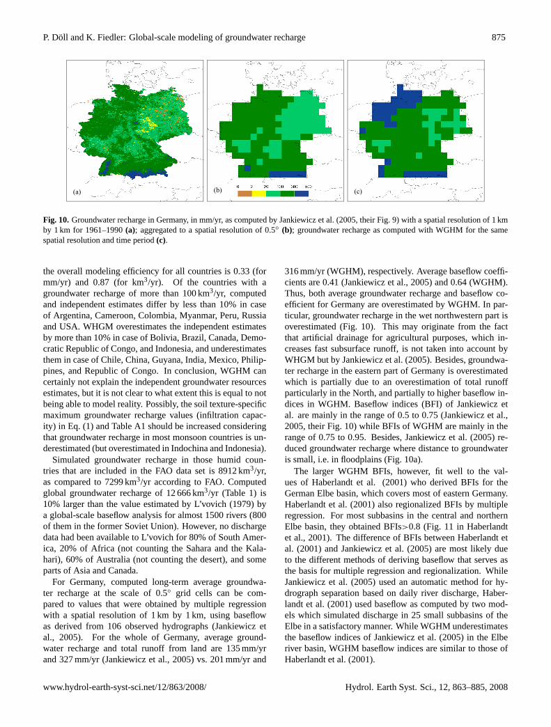
Fig. 10. Groundwater recharge in Germany, in mm/yr, as computed by Jankiewicz et al. (2005, their Fig. 9) with a spatial resolution of 1 kmby 1 km for 1961–1990(a); aggregated to a spatial resolution of 0.5◦ (b); groundwater recharge as computed with WGHM for the samespatial resolution and time period(c).
the overall modeling efficiency for all countries is 0.33 (formm/yr) and 0.87 (for km3/yr). Of the countries with agroundwater recharge of more than 100 km3/yr, computedand independent estimates differ by less than 10% in caseof Argentina, Cameroon, Colombia, Myanmar, Peru, Russiaand USA. WHGM overestimates the independent estimatesby more than 10% in case of Bolivia, Brazil, Canada, Demo-cratic Republic of Congo, and Indonesia, and underestimatesthem in case of Chile, China, Guyana, India, Mexico, Philip-pines, and Republic of Congo. In conclusion, WGHM cancertainly not explain the independent groundwater resourcesestimates, but it is not clear to what extent this is equal to notbeing able to model reality. Possibly, the soil texture-specificmaximum groundwater recharge values (infiltration capac-ity) in Eq. (1) and Table A1 should be increased consideringthat groundwater recharge in most monsoon countries is un-derestimated (but overestimated in Indochina and Indonesia).
Simulated groundwater recharge in those humid coun-tries that are included in the FAO data set is 8912 km3/yr,as compared to 7299 km3/yr according to FAO. Computedglobal groundwater recharge of 12 666 km3/yr (Table 1) is10% larger than the value estimated by L’vovich (1979) bya global-scale baseflow analysis for almost 1500 rivers (800of them in the former Soviet Union). However, no dischargedata had been available to L’vovich for 80% of South Amer-ica, 20% of Africa (not counting the Sahara and the Kala-hari), 60% of Australia (not counting the desert), and someparts of Asia and Canada.
For Germany, computed long-term average groundwa-ter recharge at the scale of 0.5◦ grid cells can be com-pared to values that were obtained by multiple regressionwith a spatial resolution of 1 km by 1 km, using baseflowas derived from 106 observed hydrographs (Jankiewicz etal., 2005). For the whole of Germany, average ground-water recharge and total runoff from land are 135 mm/yrand 327 mm/yr (Jankiewicz et al., 2005) vs. 201 mm/yr and
316 mm/yr (WGHM), respectively. Average baseflow coeffi-cients are 0.41 (Jankiewicz et al., 2005) and 0.64 (WGHM).Thus, both average groundwater recharge and baseflow co-efficient for Germany are overestimated by WGHM. In par-ticular, groundwater recharge in the wet northwestern part isoverestimated (Fig. 10). This may originate from the factthat artificial drainage for agricultural purposes, which in-creases fast subsurface runoff, is not taken into account byWHGM but by Jankiewicz et al. (2005). Besides, groundwa-ter recharge in the eastern part of Germany is overestimatedwhich is partially due to an overestimation of total runoffparticularly in the North, and partially to higher baseflow in-dices in WGHM. Baseflow indices (BFI) of Jankiewicz etal. are mainly in the range of 0.5 to 0.75 (Jankiewicz et al.,2005, their Fig. 10) while BFIs of WGHM are mainly in therange of 0.75 to 0.95. Besides, Jankiewicz et al. (2005) re-duced groundwater recharge where distance to groundwateris small, i.e. in floodplains (Fig. 10a).
The larger WGHM BFIs, however, fit well to the val-ues of Haberlandt et al. (2001) who derived BFIs for theGerman Elbe basin, which covers most of eastern Germany.Haberlandt et al. (2001) also regionalized BFIs by multipleregression. For most subbasins in the central and northernElbe basin, they obtained BFIs>0.8 (Fig. 11 in Haberlandtet al., 2001). The difference of BFIs between Haberlandt etal. (2001) and Jankiewicz et al. (2005) are most likely dueto the different methods of deriving baseflow that serves asthe basis for multiple regression and regionalization. WhileJankiewicz et al. (2005) used an automatic method for hy-drograph separation based on daily river discharge, Haber-landt et al. (2001) used baseflow as computed by two mod-els which simulated discharge in 25 small subbasins of theElbe in a satisfactory manner. While WGHM underestimatesthe baseflow indices of Jankiewicz et al. (2005) in the Elberiver basin, WGHM baseflow indices are similar to those ofHaberlandt et al. (2001).
876 P. Doll and K. Fiedler: Global-scale modeling of groundwater recharge
Fig. 11.Baseflow indices at discharge observation stations in Southern Africa, mapped onto the pertaining basins (Bullock et al., 1997, theirFig. 4.35) (left); groundwater recharge as a fraction of total runoff from land as computed with WGHM, with polygon outlines of Bullock etal. (1997) for easier comparison (right). Please note that the polygon outlines are not basin boundaries but boundaries of polygon with thesame color in the figure on the left.
Finally, WGHM baseflow coefficients for Southern Africaare compared to baseflow indices from hydrograph separa-tion at discharge observation stations in Southern Africa,mapped onto the pertaining basins (Bullock et al., 1997, theirFig. 4.35). However, on their figure, the basin outlines can-not be recognized such that it is not possible to show thecorresponding pattern of average WGHM baseflow indicesfor the basins. Figure 11 shows how the baseflow indicesas computed for individual grid cells by WGHM compare tothe average basin BFIs of Bullock et al. (1997). The col-ors of small polygons can be compared most directly, whilefor larger polygons, the grid cell values within the polygonmust be averaged. The spatial pattern of BFI on both mapsis somewhat consistent, with values below 0.1 in the west-ernmost basins in Namibia and values between 0 and 0.3in southern and eastern central South Africa. Towards themore humid North, in Angola and Zambia, both maps showlarger BFI values, but WHGM values remain between 0.6–0.8 while the Bullock et al. values are above 0.8.
Groundwater recharge as computed by WGHM (usingGPCC precipitation data) has been included in WHYMAPGlobal Map of Groundwater Resources (with some smooth-ing for cartographic reasons). During the map developmentprocess, groundwater recharge values were commented onby more than 30 groundwater experts from all around theglobe (W. Struckmeier, personal communication, 2008). Asa result, the depicted groundwater recharge was increased intwo karst areas in former Yugoslavia and in Mexico. Other-wise, the experts did not identify, in the regions they were fa-miliar with, any divergences from the groundwater rechargevalues they considered plausible.
5 Conclusions
The global 0.5◦ by 0.5◦ data set of long-term average ground-water recharge presented here is unique in that it combinesstate-of-the-art global scale hydrological modeling with in-dependent information on small-scale groundwater rechargein semi-arid and arid areas in an ensembles approach whichtakes into account and quantifies the uncertainty due to avail-able precipitation data. Basin-specific tuning of the Water-GAP Global Hydrology Model WGHM against river dis-charge at 1235 stations world-wide helps to compute reason-able estimates of total runoff from land. Inclusion of a largenumber of spatially variable climatic and physio-geographiccharacteristics (including land cover, soil water holding ca-pacity, soil texture, relief, hydrogeology, permafrost/glacier)allows a well-founded estimate of groundwater recharge dis-tribution. Consideration of reliable information on long-termaverage groundwater recharge at selected semi-arid locationsworld-wide made it possible to obtain an unbiased estimateof groundwater recharge in semi-arid areas. Finally, usingthe mean of two groundwater recharge estimates as obtainedby applying two different and equally uncertain global pre-cipitation data sets make the resulting groundwater rechargedata set more robust, while at the same time uncertainty esti-mates are provided.
Due to the scarcity of reliable independent informationon groundwater recharge at all scales, but particularly atthe scale of countries or subnational units, it is difficult tojudge how well the computed groundwater recharge esti-mates correspond to reality. In particular, a comparison tocountry estimates of groundwater resources as compiled byFAO (2005) does not help. In most cases the method of es-timation is unknown and likely to be very rough, while in
P. Doll and K. Fiedler: Global-scale modeling of groundwater recharge 877
some cases the listed renewable groundwater resources areobviously not defined as being equivalent to groundwaterrecharge. A comparison of independent estimates of ground-water recharge or rather baseflow coefficients that were de-rived using well-founded scientific methods (Jankiewicz etal., 2005; Haberlandt et al., 2005) showed that uncertaintyof baseflow estimation from river discharge may lead to sig-nificantly different estimates of meso-scale baseflow indicesand thus groundwater recharge. At the global scale, WGHMwould overestimate groundwater recharge by about 10–20%if the base-flow derived estimates of L’vovich (1979) and theFAO country values were to be trusted.
A problem with the WGHM groundwater recharge esti-mation method is that there are sharp boundaries betweensemi-arid/arid and humid zones which lead to rather abruptreductions of computed groundwater recharge at the bound-aries. In semi-arid zones close to the boundaries groundwaterrecharge may be underestimated (unless soil texture is fine).
In the future, artificial drainage will be taken into ac-count based on a global data set of artificially drainedagricultural areas (spatial resolution 0.5◦) because ground-water recharge is reduced in these areas. According tothe data set of Feick et al. (2005), 1.67 million km2 aredrained world-wide, i.e. 1.2% of the global land area withoutGreenland and Antarctica. Further validation and improve-ment of the WGHM groundwater recharge model requiresan increased number of reliable estimates of groundwaterrecharge. A large number of independent estimates of small-scale groundwater recharge in semi-arid areas, compiled byScanlon et al. (2006), will be evaluated. Validation and im-proved modeling of groundwater recharge in humid areas ishampered by uncertainties of hydrograph separation.
The presented diffuse groundwater recharge estimates canbe regarded as renewable groundwater resources. It is impor-tant to note, however, that exploitation of the total groundwa-ter recharge of an aquifer is not possible without very strongimpacts on ecosystems and other water users. Withdrawal ofa sizeable part of the groundwater recharge already leads tosignificant drawdown of the water table, with ensuing con-sequences e.g. for wetlands, and a decrease of streamflow.Thus groundwater recharge is the uppermost limit of sustain-ably exploitable groundwater resources.
Table A1. Slope classes and the relief-related groundwater rechargefactor.
Description of factors in the groundwaterrecharge model of WGHM
The following sections describe how the factors in thegroundwater recharge model as given by Eq. (1) have beenquantified, providing methods and data sources.
A1 Relief
Based on the GTOPO30 digital elevation model with a reso-lution of around 1 km (USGS EROS data center), IIASA pro-duced a map of slope classes with a resolution of 5 min (dataprovided by Gunther Fischer, February 1999) which includesthe fraction of each cell that is covered by a certain slopeclass. Seven slope classes are distinguished (Table A1). The5-min-map was aggregated and mapped onto the 0.5◦
×0.5◦
land mask, such that the percentage of each slope class withrespect to the total land area of each 0.5◦ cell is produced.An “average relief”ravg , ranging from 10 to 70, is computedas
ravg =
7∑i=1
slope classi ∗ 10∗ fraci (A1)
frac i = areal fraction of slope classi within the 0.5◦ cell.The relief-related groundwater recharge factorfr for each
slope class is given in Table A1. For each cell with an averagerelief ravg, the respective value forfr is obtained by linearinterpolation.
A2 Texture
Soil texture does not only determine the factorft in Eq. (1),but also the maximum infiltration rateRg max. Soil textureis derived from the FAO Digital Soil Map of the World andDerived Soil Properties (FAO, 1995). The digital map shows,for each 5′ by 5′ raster cell, the soil mapping unit. For eachof the 4931 soil mapping units, the following information isprovided:
878 P. Doll and K. Fiedler: Global-scale modeling of groundwater recharge
Table A2. Soil texture classes and the texture-related groundwater recharge factors.
FAO soil texture class texture valueRg max[mm/d]
ft
coarse:sands, loamy sands and sandy loams with less than 18% clay and morethan 65% sand
10 5 1
medium:sandy loams, loams, sandy clay loams, silt loams, silt, silty clay loamsand clay loams with less than 35% clay and less than 65% sand; the sandfraction may be as high as 82% if a minimum of 18% clay is present
20 3 0.95
fine:clays, silty clays, sandy clays, clay loams and silty clay loams with morethan 35% clay
30 1.5 0.7
rock or glacier (in 100% of cell land area) 1 0 0
Table A3. Hydrogeological units relevant for groundwater recharge and the aquifer-related groundwater recharge factors.
Hydrogeological units unit fa fa in hot andhumid climates∗
Cenozoic and Mesozoic sediments 1 1 1with high hydraulic conductivityPaleozoic and Precambrian sediments y 2 0.7 0.8with low hydraulic conductivitnon-sedimentary rocks with 3 0.5 0.7very low hydraulic conductivity
∗ Average annual temperature more than 15◦C and average annual precipitation more than 1000 mm (average climatic conditions 1961–1990).
– names of up to 8 soil units that constitute the soil map-ping unit
– the area of each soil unit in percent of the total area ofthe soil mapping unit
– the area of each soil unit belonging to one of three tex-ture classes and to one of three slope classes
The soil texture provided by FAO is only representative forthe uppermost 30 cm of the soil. We assigned a texture valueof 10 to coarse texture, a value of 20 to medium and a value of30 to fine texture (Table A2). Based on the FAO information,an areally weighted average texture value was computed forthe 5′ cells, which was then averaged for land area of each0.5◦ cell. For the following soil units, texture was not given:dunes, glacier, bare rock, water, and salt. The texture valueof dunes was set to 10. All other four soil unit types werenot taken into account for computing the areal averages (thebare rock extent in the FAO data set appears to be much toosmall). Therefore, in a cell with e.g. 20% water or bare rock,the texture value of the cell is 15 if 40% of the area is coveredwith coarse soils and 40% with medium soils. If the total
cell area is water, the texture value is set to 0; if it is barerock or glacier (only very few cells), the texture value equals1. In these cases, surface runoff is assumed to be equal tototal runoff. For some cells (Greenland and some islands),no texture data are provided by FAO. In this case, the texturewas assumed to have a texture value of 20.
A3 Hydrogeology
A global hydrogeological map does not exist. Only for Eu-rope and Africa, there are hydrogeological maps, which,however, use very different classifications. The Hydroge-ological Map of Pan-Europe (RIVM, 1991) distinguishesamong areas with good, modest, poor and no hydraulic con-ductivity. A hydrogeological map of Africa (UN, 1988)was derived from a geological map and only gives infor-mation on porosity but not on the more important hydraulicconductivity. A map of groundwater resources in Africa(UNDTCD, 1988) provides additional information on exten-sive unconfined and confined sedimentary aquifers and local,fragmented fractured aquifers.
P. Doll and K. Fiedler: Global-scale modeling of groundwater recharge 879
Table A4. Permafrost extent classes.
Permafrost extent class according to originalCpg corresponding to fpg
permafrost map each class [%]
continuous extent of permafrost (90–100%) 95 0.05discontinuous extent of permafrost (50–90%) 70 0.3sporadic extent of permafrost (10–50%) 30 0.7isolated patches of permafrost (0–10%) 5 0.95areas without occurrence of permafrost 0 1glacier 100 0
On the global scale, only geological maps do exist. Thedigital Generalized Geological Map of the World (Cana-dian Geological Survey, 1995) provides, on a scale of 1:35million, information on the rock type and the rock age.Rock type classes are “mainly sedimentary”, “mainly vol-canic”, “mixed sedimentary”, “volcanic and volcaniclasticplutons”, “intrusive and metamorphic terranes”, “tectonicassemblages, schist belts and melanges”, “ice cap (Green-land)”. From this map, the dominant rock type and rock agefor the land area of each 0.5◦
×0.5◦ cell was assigned to therespective cell.
However, this rock type classification is not very helpfulfor estimating where groundwater recharge is relatively highand where not, as rock type classes only show a low corre-lation with the hydraulic conductivity of the rock. In partic-ular, sedimentary rocks include both sands and clays, whichhave extremely different hydraulic conductivities. For non-sedimentary rocks, the degree of fracturing is decisive for thehydraulic conductivity, and this information is not given ei-ther. For Europe, the rock types in combination with the rockages were compared to the Hydrogeological Map of Pan-Europe. It appears that all rock types except the type “mainlysedimentary” correlate to some degree with areas of poor orno hydraulic conductivity. The “mainly sedimentary” rocktype corresponds mainly to good or modest hydraulic con-ductivity if the rock age is either Cenozoic or Mesozoic. Pa-leozoic sedimentary rocks can have any hydraulic conductiv-ity, while Precambrian sedimentary rocks mostly have pooror no permeability. Based on this comparison to the Hy-drogeological Map of Pan-Europe, only a very rough clas-sification of hydrogeological units relevant for groundwaterrecharge appears to be appropriate (Table A3). This clas-sification was checked against the maps for Africa, and nosystematic error became apparent.
High temperature and precipitation enhances weathering.Therefore, groundwater recharge is assumed to be higher inwarm and humid climates. The aquifer-related recharge fac-torsfa are modified based on the long-term (1961–1990) av-erage annual temperature and precipitation in each cell (Ta-ble A3).
A4 Permafrost and glaciers
It is assumed that there is no groundwater recharge in the caseof permafrost and glaciers. Therefore, a data set was pro-duced that provides the percentage of the land area of eachcell that is underlain by permafrost or covered by glaciers.The higher this percentage is the smaller is the fraction oftotal runoff that recharges the groundwater.
Brown et al. (1998) provide digital data for the extentof permafrost on the Northern Hemisphere, including in-formation on glaciers in North America and the Arctic is-lands (like Spitzbergen and Nowaja Semlja). Table A4 liststhe five classes of permafrost extent according to Brown etal. (1998). To each of the five classes, an exact percentageof the area affected by permafrostCpg was assigned, andfpg was set to (100-Cpg)/100. For North America and theArctic islands, some map units within permafrost areas arenot assigned to any permafrost extent class but are classifiedas glaciers. However, on the rest of the map, e.g. in Nor-way or in the Himalayas, no information on glaciers is given,and the permafrost areas are continuous. The glacier areas inNorth America and the Arctic islands were assigned a valueof Cpg=100%.
The permafrost map was rasterized on a grid of1/18◦
×1/18◦, each cell being assigned to one of the fiveclasses in Table A4 or to the class “glacier”. Then, the arealpercentage of permafrost and glacier coverage within each0.5◦ cell was determined as the average of theCpg-valuesof the 1/18◦×1/18◦ cells that are land cells on Brown etal. (1998) map.
For the Southern Hemisphere, no reliable maps of per-mafrost areas could be found, which is due to the sporadicoccurrence of permafrost and the little research done. Thus,the impact of permafrost on groundwater recharge was ne-glected for the Southern Hemisphere.
In the next step, the glacier coverage for the land ar-eas outside North America and the Arctic was added. Theglacier coverage was derived from the World Glacier In-ventory (Hoelzle and Haeberli, 1999); in this inventory, theapproximate location of the center of each glacier and itsareal extent is provided. Glaciers with an areal extent of at
880 P. Doll and K. Fiedler: Global-scale modeling of groundwater recharge
least 1 km2 were taken into account, which resulted in 8998glaciers globally (outside North America and the Arctic is-lands, and not considering Greenland and the Antarctic). Foreach 0.5◦ cell, the areal extents of all glaciers located withinthe cell were summed up. When a cell only has glaciers andno permafrost, the fraction of the glacial area with respect tothe total land area of the cells is equal to the valueCpg. Ifthere are both permafrost and glaciers (outside North Amer-ica and the Arctic islands) within a 0.5◦ cell,Cpg is computedas
Cpg =100∗ Agl + Cpg(permafrost) ∗ (Aland − Agl)
Aland(A2)
Agl = sum of all glacial area in a 0.5◦ cell [km2]Cpg(permafrost) = averageCpg-value due to permafrostAland = land area of 0.5◦ cell [km2]
The factorfpg is assumed to be linearly related toCpg,with fpg=1 if Cpg=0% (no decrease of groundwater rechargedue to glaciers and permafrost if neither of them occurs) andfpg=0 if Cpg=100% (no groundwater recharge if the cell istotally covered by glaciers).
Appendix B
Renewable groundwater resources and totalrenewable water resources of countries as computedby WGHM for the climate normal 1961–1990
The internally renewable water resources of countries areequal to the difference of long-term average precipitation andevapotranspiration within a country. In semi-arid countries,it can be negative if inflow from other countries evapotranspi-rates within the country. The internally renewable groundwa-ter resources are equal to the groundwater recharge within thecountries; they are always positive. In Table B1, the meansof the total and groundwater resources computed with GPCCand CRU precipitation data for 1961–1990 are listed togetherwith the percent deviation from the mean (difference betweenresources as computed with either one of the two precipita-tion data sets and the ensemble mean value), which shows theuncertainty of the model estimates due to the uncertain pre-cipitation input data. B/A represents groundwater resourcesin percent of total water resources. In some semi-arid coun-tries, it can be larger than 100% or negative because totalwater resources are reduced by evapotranspiration from sur-face water bodies. Only countries with an area of more than10 000 km2 are listed.
884 P. Doll and K. Fiedler: Global-scale modeling of groundwater recharge
Acknowledgements.The authors are grateful for the contribution ofM. Edmunds, University of Oxford, who compiled the estimates oflocal groundwater recharge in semi-arid and arid regions around theworld. They thank M. Florke, University of Kassel, for her inputwith respect to model modification in semi-arid and arid region,and K. Verzano, University of Kassel, and M. Hunger, FrankfurtUniversity, for their programming work. Part of the researchpresented in this publication was funded by the InternationalAtomic Energy Agency (IAEA), Vienna.
Edited by: K. Bishop
References
Adam, J. C. and Lettenmeier, D. P.: Adjustment of global grid-ded precipitation for systematic bias, J. Geophys. Res.-Atmos.,108(D9), 4257, doi:10.1029/2002JD002499, 2003.
Alcamo, J., Doll, P., Henrichs, T., Kaspar, F., Lehner, B., Rosch,T., and Siebert, S.: Development and testing of the WaterGAP2 global model of water use and availability, Hydrol. Sci., 48,317–337, 2003.
Brown, J., Ferrians Jr., O. J., Heginbottom, J. A., and Melnikov,E. S.: Digital Circum-Arctic Map of Permafrost and Ground-IceConditions, International Permafrost Association Data and Infor-mation Working Group, Circumpolar Active-Layer PermafrostSystem (CAPS), CD-ROM version 1.0. National Snow and IceData Center, University of Colorado, Boulder, 1998.
Bullock, A., Andrew, A., and Mngodo, R.: Regional surface waterresources and drought assessment, in: UNESCO Tech. Doc. inHydrol. No. 15, Southern African FRIEND, Paris, 40–93, 1997.
Canadian Geological Survey: Generalized Geological Map of theWorld and Linked Databases, Open File Report 2915d, CD-ROM, 1995.
CIESIN (Center for International Earth Science Information Net-work): Gridded Population of the World Version 3 (GPWv3):Population Grids, Palisades, NY: Socioeconomic Data and Ap-plications Center (SEDAC), Columbia University,http://sedac.ciesin.columbia.edu/gpw, 2005.
Dirmeyer, P. A., Gao, X.., Zhao, M., Guo, Y., Oki, T., and Hanasaki,N.: The Second Global Soil Wetness Project (GSWP-2): Multi-Model Analysis and Implications for our Perception of the LandSurface, COLA Technical Report,ftp://grads.iges.org/pub/ctr/ctr 185.pdf, 2005.
Doll, P. and Florke, M.: Global-Scale Estimation of DiffuseGroundwater Recharge, Frankfurt Hydrology Paper 03, Instituteof Physical Geography, Frankfurt University, Frankfurt am Main,2005.
Doll, P., Kaspar, F., and Lehner, B.: A global hydrological modelfor deriving water availability indicators: model tuning and vali-dation, J. Hydrol., 270, 105–134, 2003.
Doll, P. and Lehner, B.: Validation of a new global 30-min drainagedirection map, J. Hydrol., 258, 214–231, 2002.
Doll, P. and Siebert, S.: Global modeling of irrigationwater requirements, Water Resour. Res., 38, 8.1–8.10,doi:10.1029/2001WR000355, 2002.
Doll, P., Lehner, B., and Kaspar, F.: Global modeling of groundwa-ter recharge, in: Proceedings of Third International Conferenceon Water Resources and the Environment Research, edited by:
Schmitz, G. H., Technical University of Dresden, Germany, I,27–31, 2002.
ESRI (Environmental Systems Research Institute): Data and Maps2004, 2004.
FAO (Food and Agriculture Organization of the United Nations):Digital Soil Map of the World and Derived Soil Properties, CD-ROM version 3.5, 1995.
FAO (Food and Agriculture Organization of the United Nations):Review of world water resources by country, FAO Water ReportNo. 23, Rome, 2003.
FAO (Food and Agriculture Organization of the United Nations),Land and Water Development Division: AQUASTAT onlinedatabase, including water resources per country,http://www.fao.org/nr/water/aquastat/dbase/index.stm, 2005.
Feick, S., Siebert, S., and Doll, P.: A Digital Global Map of Ar-tificially Drained Agricultural Areas, Frankfurt Hydrology Pa-per 04, Institute of Physical Geography, Frankfurt University,Frankfurt am Main,http://www.geo.uni-frankfurt.de/ipg/ag/dl/publikationen/index.html, 2005.
Fuchs, T., Schneider, U., and Rudolf, B.: Global precip-itation analysis products of GPCC, GPCC/Deutscher Wet-terdienst,http://www.dwd.de/en/FundE/Klima/KLIS/int/GPCC/ReportsPublications/QR/GPCCintro products2007.pdf, 2007.
Guntner, A., Stuck, J., Werth, S., Doll, P., Verzano, K., andMerz, B.: A global analysis of temporal and spatial variationsin continental water storage, Water Resour. Res., 43, W05416,doi:10.1029/2006WR005247, 2007a.
Guntner, A., Schmidt, R., and Doll, P.: Supporting large-scale hy-drogeological monitoring and modelling by time-variable grav-ity data, Hydrogeol. J., 15, 167–170, doi:10.1007/s10040-006-0089-1, 2007b.
Guo, Z., Dirmeyer, P.A., Hu, Z.-Z., Gao, X., and Zhao, M.: Evalu-ation of the Second Global Soil Wetness Project soil moisturesimulations: 2. Sensitivity to external meteorological forcing,J. Geophys. Res., 111, D22S03, doi:10.1029/2006JD007845,2006.
Haberlandt, U., Klocking, B., Krysanova, V., and Becker, A.: Re-gionalisation of the base flow index from dynamically simulatedflow components – a case study in the Elbe River Basin, J. Hy-drol., 248, 35–53, 2001.
Hevesi, J. A., Flint, A. L., and Flint, L. E.: Simulation of Net In-filtration and Potential Recharge Using a Distributed-ParameterWatershed Model of the Death Valley Region, Nevada and Cal-ifornia, USGS Water-Resources Investigations Report 03-4090,Sacramento, 2003.
Hoelzle, M. and Haeberli, W.: World Glacier Inventory. WorldGlacier Monitoring Service, National Snow and Ice Data Cen-ter, University of Colorado, Boulder, 1999.
Hunger, M. and Doll, P.: Value of river discharge data for global-scale hydrological modeling, Hydrol. Earth Syst. Sci., 12, 841–861, 2008,http://www.hydrol-earth-syst-sci.net/12/841/2008/.
Jankiewicz, P., Neumann, J., Duijnisveld, W. H. M., Wessolek,G., Wycisk, P., and Hennings, V.: Abflusshohe, Sickerwasser-rate, Grundwasserneubildung – Drei Themen im HydrologischenAtlas von Deutschland, Hydrologie und Wasserbewirtschaftung,49, 2–13, 2005.
Janssen, P. H. M. and Heuberger, P. S. C.: Calibration of process-oriented models, Ecol. Model., 83, 55-66, 1995.
P. Doll and K. Fiedler: Global-scale modeling of groundwater recharge 885
Keese, K. E., Scanlon, B. R., and Reedy, R. C.: Assess-ing controls on diffuse groundwater recharge using unsat-urated flow modeling, Water Resour. Res., 41, W06010,doi:10.1029/2004WR003481, 2005.
Lavapuro, M., Lipponen, A., and Artimo, A.: Groundwater sus-tainability indicators: testing with Finnish data, in: Groundwaterresources sustainability indicators, edited by: Vrba, J. and Lip-ponen, A., IHP-VI Series on Groundwater No. 14, UNESCO,52–72, 2007.
Legates, D. R.: A climatology of global precipitation, Publ.Climatol., 40(1), Center for Climatic Research, University ofDelaware, 1987.
Lerner, D. N., Issar, A. S., and Simmers, I.: Groundwater recharge:a guide to understanding and estimating natural recharge, In-ternational Contributions to Hydrogeology, 8, Heise, Hannover,1990.
L’vovich, M. I.: World Water Resources and their Future. AmericanGeophysical Union, Washington D.C., 1979.
Margat, J.: Les Eaux Souterraines dans le Monde, BRGM R31780,Orleans, 1990.
Mitchell, T. D. and Jones, P. D.: An improved method of construct-ing a database of monthly climate observations and associatedhigh-resolution grids, Int. J. Climatol., 25, 693–712, 2005.
Neumann, J.: Flachendifferenzierte Grundwasserneubildung vonDeutschland – Entwicklung und Anwendung des makroskali-gen Verfahrens HAD-GW Neu, Dissertation, Martin-Luther-Universitat Halle-Wittenberg, ULB Sachsen-Anhalt, 137 pp.,2005.
New, M., Hulme, M., and Jones, P. D.: Representing twentiethcentury space–time climate variability, Part 1: development ofa 1961–90 mean monthly terrestrial climatology, J. Climate, 12,829–856, 1999.
New, M., Hulme, M., and Jones, P. D.: Representing twentieth cen-tury space-time climate variability, Part 2: development of 1901–96 monthly grids of terrestrial surface climate, J. Climate, 13,2217–2238, 2000.
Scanlon, B. R., Keese, K. E., Flint, A. L., Flint, L. E., Gaye, C. B.,Edmunds, W. M., and Simmers, I.: Global synthesis of ground-water recharge in semiarid and arid regions, Hydrol. Processes,20, 3335–3370, 2006.
Scanlon, B. R., Healy, R. W., and Cook, P. G.: Choosing appropriatetechniques for quantifying groundwater recharge, Hydrogeol. J.,10, 18–39, 2002.
Seguin, J. J.: Hydrogeological Map of Africa: a prototype at1/10 M scale, Baureau des Recherches Geologiques et Minieres(BGRM)/Service Eau, France, 2005.
Simmers, I.: Recharge of phreatic aquifers in (semi-)arid areas, A.A. Balkema, Rotterdam, 1997.
Small, E. E.: Climatic controls on diffuse groundwater recharge insemiarid environments of the southwestern United States, WaterResour. Res., 41, W04012, doi:10.1029/2004WR003193, 2005.
Tallaksen, L. M.: A review of baseflow recession analysis, J. Hy-drol., 165, 349–370, 1995.
UNEP (United Nations Environment Programme): World Atlas ofDesertification, 1992.
Vassolo, S. and Doll, P.: Global-scale gridded estimates of thermo-electric power and manufacturing water use, Water Resour. Res.,41, W04010, doi:10.1029/2004WR003360, 2005.
Vogel, J. C. and Van Urk, H.: Isotopic composition of groundwaterin semi-arid regions of southern Africa, J. Hydrol., 25, 23–26,1975.
WRI (World Resources Institute): EarthTrends Water Resourcesand Freshwater Ecosystems Data Tables, Freshwater Re-sources 2005,http://earthtrends.wri.org/pdflibrary/datatables/wat2 2005.pdf, 2005a.
WRI (World Resources Institute): EarthTrends Water Resourcesand Freshwater Ecosystems Searchable Database, Internal Re-newable Water Resources (IRWR): Groundwater recharge, vol-ume,http://earthtrends.wri.org/searchabledb/index.php?theme=2, 2005b.
WRI (World Resources Institute): World Resources 2000–2001 –People and ecosystems: The fraying web of life, 2000.
WRI (World Resources Institute): EarthTrends Water Resourcesand Freshwater Ecosystems Data Tables, Groundwater andDesalinization 2000,http://earthtrends.wri.org/pdflibrary/datatables/fw2n2000.pdf, 2000.