Rupture Process of the Great 2004 Sumatra-Andaman Earthquake

Supporting Online Materials

Submitted to Science, March 12, 2005

Charles J. Ammon1, Ji Chen2, Hong-Kie Thio3, David Robinson5, Sidao Ni5,2, Vala

Hjorleifsdottir2, Hiroo Kanamori2, Thorne Lay3, Shamita Das5, Don Helmberger2, Gene

Ichinose3, Jascha Polet5, David Wald7

Materials and Methods

Global Seismic Wavefield Observations and SEM Seismograms

We computed the global wavefield excited by Model III using the spectral element

method (SEM) (1) for a 3D Earth model composed of mantle model s20rts (1), model

Crust 2.0 (2), and topography from ETOPO5. We show the predicted velocities and

displacements on the Earth’s surface as movies. The 3D simulations were used to

calibrate the effect of 3D structure on the 1D waveforms used in the inversion for Model

III. By comparing the fits of synthetics computed for different models to data that were

not used in the inversions these synthetics can be used to distinguish between models.

This was done qualitatively when developing model III to estimate the improvements

between successive versions of the model. The waveforms for model III match the

overall amplitude and directivity in observed seismograms (Fig. S1) over a wide

1Department of Geosciences, The Pennsylvania State University, 440 Deike Building, University Park, PA

16802, USA. 2Seismological Laboratory, California Institute of Technology, MS 252-21, Pasadena, CA

91125, USA. 3Earth Sciences Department, University of California, Santa Cruz, CA 95064, USA. 4URS

Corporation, 566 El Dorado Street, Pasadena, CA 91101, USA. 5Department of Earth Sciences, University

of Oxford, Parks Road, Oxford OX1 3PR, UK. 6Institute for Crustal Studies, Santa Barbara, CA, USA., 7National Earthquake Information Center, US Geological Survey, Golden, CO 80401, USA.

Ammon et al., 2005 Supplements 4/27/05

frequency range. We also provide a dynamic view of regional and global seismic ground

motions in Movies S1 and S2. The SEM simulations were performed on 150-196

processors of Caltech’s Division of Geological and Planetary Sciences Dell cluster.

Surface Deformation

The surface deformation predicted by the finite fault models provides important

information on the tsunami source, and may provide a means of independently verifying

the source-modeling results as the sea-floor is mapped in more detail. We present two

views of the surface slip: a static map of the slip produced by the event (Fig S2), and a

movie that shows the evolution of the surface slip during the rupture (Movie S3).

Long-Period Rayleigh Wave Directivity

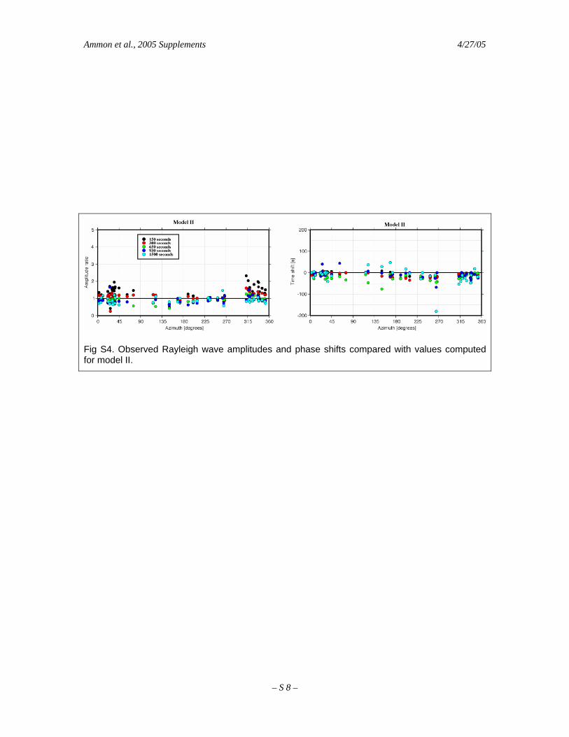
The amplitude ratios and phase shifts are computed as follows. Both observed and

synthetic records are band-pass filtered between frequencies fl and fh. Then the group

arrival time is computed using a group velocity, U. R3 wave train is used for the two

longest periods, and R1 wave train is used for the shorter periods. Then the records are

windowed centered at the group arrival time and with a duration, τ. The values of these

parameters used are listed in Table S1. Amplitude ratios (observed/synthetic) of the peak

amplitudes are then computed. The time shifts (observed - computed) are computed by

cross correlation. In the main text, we showed the results for HVD CMT and Model III,

but Model II explains the data as well, as shown in Fig S4.

R1 Source-Time-Function Analysis Supplementary Details

The R1 moment rate, or source time functions (STFs) were estimated using two different

deconvolution methods. For both methods we used a distance-dependent group-velocity

window to window R1 from the seismograms. Specifically, we used an initial group

velocity of about 7.75 km/s until the arrival of R2 (with the same group velocity). In both

instances the results are convolved with a Gaussian low-pass filter to reduce short period

noise cause by inadequate Earth models for those periods. This gives us long time

windows at close stations, and maximizes what we can use for more distance stations.

– S 2 –

Ammon et al., 2005 Supplements 4/27/05

Each method has advantages and disadvantages. The frequency-domain water-level

method has a high temporal resolution but includes substantial side lobes as a

consequence of low long-period signal-to-noise ratios. Some observations are better

handled by one method. This is particularly true of the observations in the direction

roughly opposite the direction of rupture propagation. The water-level results include

more observations in this direction. The iterative time-domain STF estimates were

computed with a positivity constraint that produces a more stable low-frequency signal

and removes side lobes. This makes these signals easier to work with in the IRT

inversion. These STFs are allowed to begin 60 seconds before the origin time. Since we

only use STFs that fit more than 80% of the observed seismic signal power when

convolved with the synthetic Green’s function, several observations are lost using this

method. The main arrivals that can be tracked across at least several time functions are

common for both methods. Although we have a large data set (more than

170 R1 observations), most are from North America and western Europe, as can be seen

from the number of observations in each bin. In future work we will incorporate R2

observations, that can help balance the north (rupture towards) and south (rupture away)

coverage.

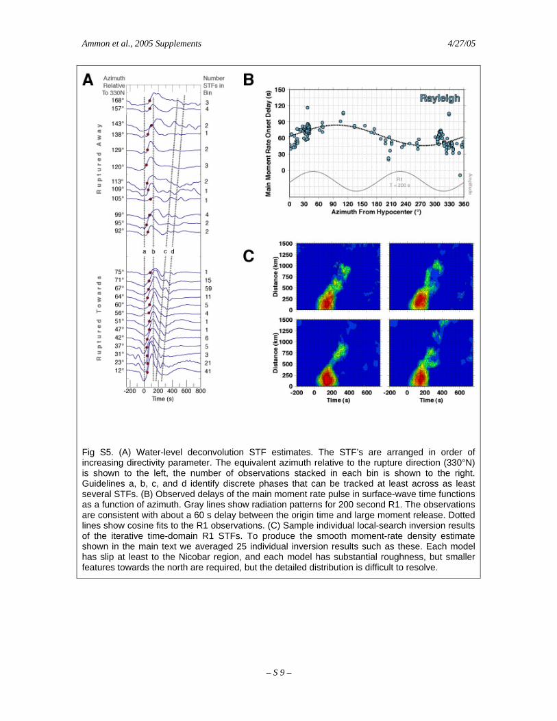
A particular interesting feature that is easily overlooked is an initial delay in the large

amplitude pulse in the moment-rate functions. For a number of the observations a small

initial pulse in the source time functions is observable starting at the USGS origin time

(zero on the time scale), but the signals are dominated by a large moment rate pulse that

begins about 60 s after the USGS origin time. There is a systematic azimuthal delay in

the onset of the strong pulse. Although not immediately apparent in Fig S5, an analysis of

the delay time associated with the largest moment-rate pulse onset suggests that the large

increase in moment rate began about 30-60 s following the event’s start. Such an increase

suggests increase in slip, an increase in the rate of rupture expansion, or both. Although

we cannot separate the two in this form of analysis, measurements on the band-limited

surface-wave moment rate functions suggest at least part of the slip contributing to the

rapid increase in moment rate was located about 50-80 km up-dip of the hypocenter.

– S 3 –

Ammon et al., 2005 Supplements 4/27/05

We model the observed variations in moment rate using an Inverse Radon Transform (2,

3). The mathematics of the procedure are straightforward and linear, once a rupture

direction is chosen. For a surface wave analysis we must choose an average phase

velocity for the Rayleigh waves – we used 4.75 km/s, but the results are very similar for a

range from 4.25 to 5.0 km/s. We can solve the linear algebra using a number of tools, and

we employed a conjugate-gradient method, which produces exceptional fits to the data

but complicates interpretation because the method is prone to streaking in tomographic

problems (4). Our preferred solution is to use a suite of linear-search inversions that

consist of two perturbation schemes. In each, we require that the moment-rate density

remain positive, and include minimum length constraints along with the constraint that

the area of all time functions be uniform (which helps suppress artifacts near the model

edges) and we minimize a weighted L1 norm of the match of the predictions to the

observations. The original moment-rate functions are binned and averaged to produce 30

source time functions. We down-weight binned STFs computed three or less

observations. For the first step of the inversion, we add Gaussian filtered random images

to the current best fitting model (beginning with a uniformly zero model); if the

perturbation improves the fit, we update the model. Through trial and error we find that

about 2000 perturbations produces a reasonable fit to the observations, although artifacts

of the perturbation scheme remain in the image. The second step of the inversion is

designed to improve the data fit, and to reduce the model size. Here we add Gaussian

“bumps” to small regions of the image in a second local search. Again, we found that

after about 2000 steps, this search has substantially reduces the artifacts from the more

global perturbation scheme. Several examples are shown in Fig S5c. To identify the

smoothest components of all solutions we average the results of 25 inversions.

Model Slip Direction Variations

Our focus on the slip models has been the slip magnitude, although each model includes

some variation in the slip direction as well. Model I includes a fixed rake on each fault

segment using the focal mechanisms information from the Harvard CMT for the main

shock and an aftershock. Rake variations for Model II are shown in Figure S6.

– S 4 –

Ammon et al., 2005 Supplements 4/27/05

Supporting Figures

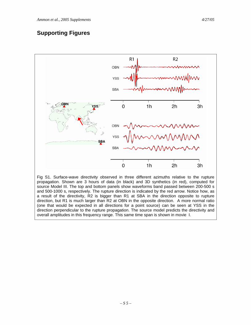
Fig S1. Surface-wave directivity observed in three different azimuths relative to the rupture propagation. Shown are 3 hours of data (in black) and 3D synthetics (in red), computed for source Model III. The top and bottom panels show waveforms band passed between 200-500 s and 500-1000 s, respectively. The rupture direction is indicated by the red arrow. Notice how, as a result of the directivity, R2 is bigger than R1 at SBA in the direction opposite to rupture direction, but R1 is much larger than R2 at OBN in the opposite direction. A more normal ratio (one that would be expected in all directions for a point source) can be seen at YSS in the direction perpendicular to the rupture propagation. The source model predicts the directivity and overall amplitudes in this frequency range. This same time span is shown in movie I.

– S 5 –

Ammon et al., 2005 Supplements 4/27/05

Fig S2. Static uplift associated with Model III are computed using the spectral element method. Contours are shown at 0.5 meter intervals. Uplift values are between one to five m across a region with dimensions of 100 km x 500 km, from the epicenter near 3°N to about 8°N. The maximum uplift is near the trench between 3°N and 5°N. This region of large uplift is consistent with that inferred from tsunami data (Paper 1).

– S 6 –

Ammon et al., 2005 Supplements 4/27/05

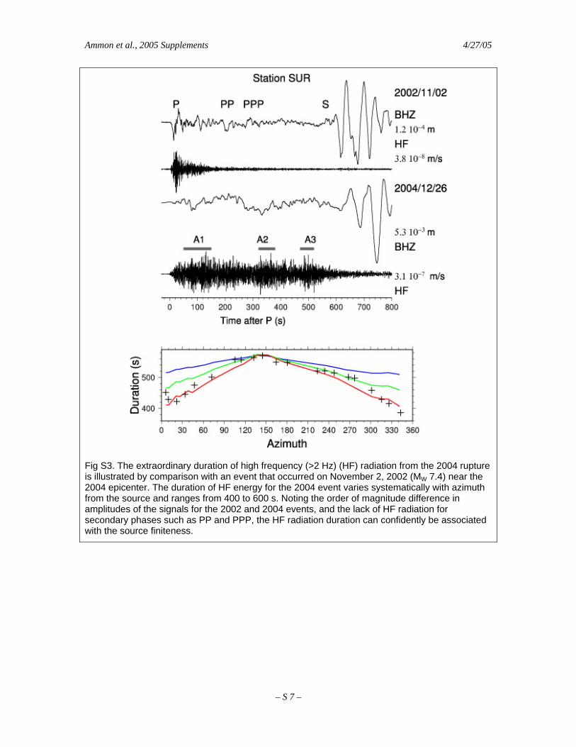
Fig S3. The extraordinary duration of high frequency (>2 Hz) (HF) radiation from the 2004 rupture is illustrated by comparison with an event that occurred on November 2, 2002 (MW 7.4) near the 2004 epicenter. The duration of HF energy for the 2004 event varies systematically with azimuth from the source and ranges from 400 to 600 s. Noting the order of magnitude difference in amplitudes of the signals for the 2002 and 2004 events, and the lack of HF radiation for secondary phases such as PP and PPP, the HF radiation duration can confidently be associated with the source finiteness.

– S 7 –

Ammon et al., 2005 Supplements 4/27/05

Fig S4. Observed Rayleigh wave amplitudes and phase shifts compared with values computed for model II.

– S 8 –

Ammon et al., 2005 Supplements 4/27/05

Fig S5. (A) Water-level deconvolution STF estimates. The STF’s are arranged in order of increasing directivity parameter. The equivalent azimuth relative to the rupture direction (330°N) is shown to the left, the number of observations stacked in each bin is shown to the right. Guidelines a, b, c, and d identify discrete phases that can be tracked at least across as least several STFs. (B) Observed delays of the main moment rate pulse in surface-wave time functions as a function of azimuth. Gray lines show radiation patterns for 200 second R1. The observations are consistent with about a 60 s delay between the origin time and large moment release. Dotted lines show cosine fits to the R1 observations. (C) Sample individual local-search inversion results of the iterative time-domain R1 STFs. To produce the smooth moment-rate density estimate shown in the main text we averaged 25 individual inversion results such as these. Each model has slip at least to the Nicobar region, and each model has substantial roughness, but smaller features towards the north are required, but the detailed distribution is difficult to resolve.

– S 9 –

Ammon et al., 2005 Supplements 4/27/05

Fig S6. Rake variation in Model II. Arrows point in the direction of hanging-wall movement (relative to the footwall).

– S 10 –

Ammon et al., 2005 Supplements 4/27/05

Fig S7. Observed and predicted SH waveform fits for the first finite fault inversion. The black lines are the observations the red lines are the predictions. Azimuth and take off angle distribution is indicated on the focal mechanism. The seismogram length varies from station-to-station depending on the time that a secondary arrival interfered with the primary SH observation. The signals were aligned by hand-picking SH onsets. Since the beginning of the SH waves was emergent, the start times were refined through multiple inversions. These optimal time shifts generally differ from the theoretical SH arrival times by only a few seconds.

– S 11 –

Ammon et al., 2005 Supplements 4/27/05

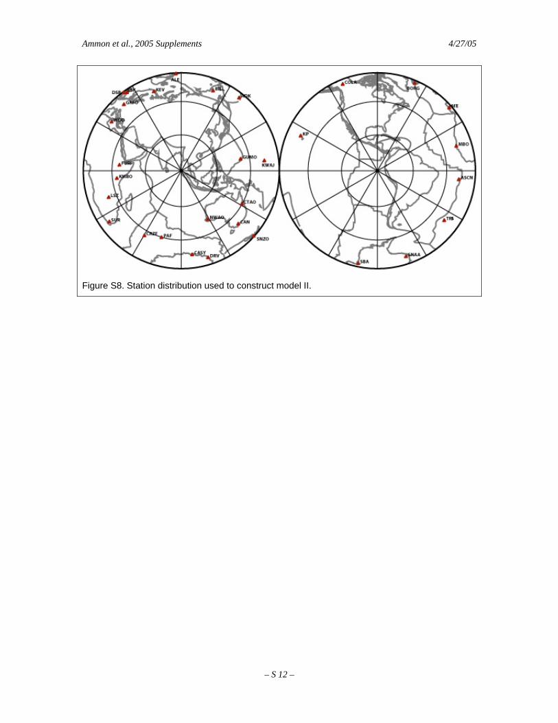
Figure S8. Station distribution used to construct model II.

– S 12 –

Ammon et al., 2005 Supplements 4/27/05

Figure S9. Surface-wave fits corresponding to Model II.

– S 13 –

Ammon et al., 2005 Supplements 4/27/05

Figure S10. Very long-period seismogram fits corresponding to Model II.

– S 14 –

Ammon et al., 2005 Supplements 4/27/05

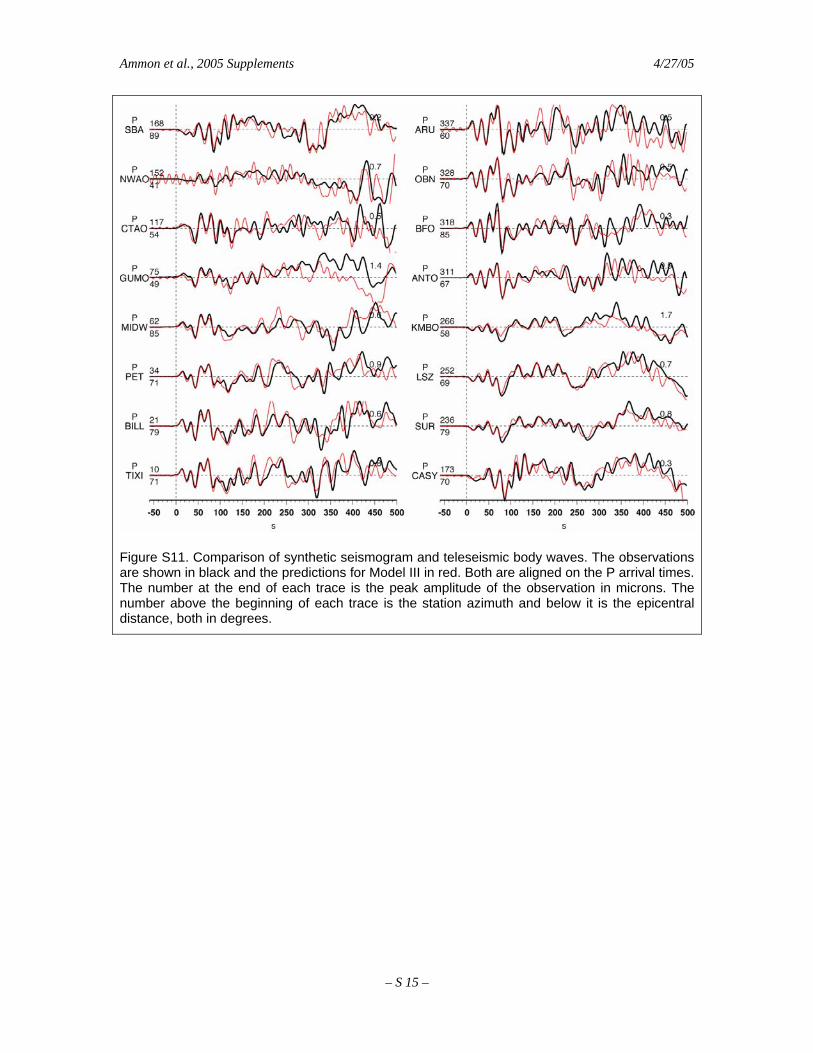
Figure S11. Comparison of synthetic seismogram and teleseismic body waves. The observations are shown in black and the predictions for Model III in red. Both are aligned on the P arrival times. The number at the end of each trace is the peak amplitude of the observation in microns. The number above the beginning of each trace is the station azimuth and below it is the epicentral distance, both in degrees.

– S 15 –

Ammon et al., 2005 Supplements 4/27/05

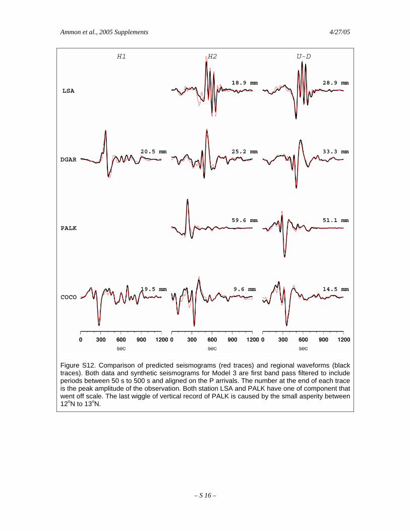
Figure S12. Comparison of predicted seismograms (red traces) and regional waveforms (black traces). Both data and synthetic seismograms for Model 3 are first band pass filtered to include periods between 50 s to 500 s and aligned on the P arrivals. The number at the end of each trace is the peak amplitude of the observation. Both station LSA and PALK have one of component that went off scale. The last wiggle of vertical record of PALK is caused by the small asperity between 12oN to 13oN.

– S 16 –

Ammon et al., 2005 Supplements 4/27/05

Figure S13. Comparison of predicted seismograms (red traces) and long period vertical waveforms (black traces). Both data and synthetic seismograms (model 3) were band pass filtered to include periods between 250 s to 2000 s using a causal Butterworth filter and then aligned on the NEIC origin time. The number at the end of each trace is the peak amplitude of the observation. We believe that the long period signals showed at records of TIXI, PET, and KMBO from 3000 sec to 5000 sec are caused by instrument problems.

– S 17 –

Ammon et al., 2005 Supplements 4/27/05

Supporting Tables

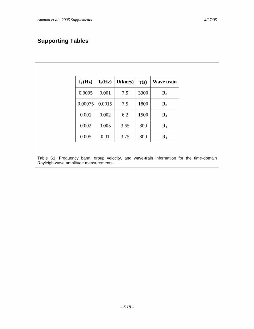
fl (Hz) fh(Hz) U(km/s) τ(s) Wave train

0.0005 0.001 7.5 3300 R3

0.00075 0.0015 7.5 1800 R3

0.001 0.002 6.2 1500 R1

0.002 0.005 3.65 800 R1

0.005 0.01 3.75 800 R1

Table S1. Frequency band, group velocity, and wave-train information for the time-domain Rayleigh-wave amplitude measurements.

– S 18 –

Ammon et al., 2005 Supplements 4/27/05

Online Movies and Animations

Movie S1: http://www.gps.caltech.edu/~vala/sumatra_velocity_global.mpeg

Movie S1. Global movie of the vertical velocity wave field. The computation includes periods of 20 s and longer and shows a total duration of 3 hours. The biggest phases seen in this movie are the Rayleigh waves traveling around the globe. Global seismic stations are shown as yellow triangles. The animation was made with the help of Santiago Lombeyda at the Center for Advanced Computing Research, Caltech.

Movie S2: http://www.gps.caltech.edu/~vala/sumatra_velocity_local.mpeg

Movie S2. Animation of the vertical velocity wave field in the source region. The computation includes periods of 12 s and longer with a total duration of about 13 minutes. As the rupture front propagates northward the wave-field gets compressed and amplified in the north, and drawn out to the south. The radiation from patches of large slip shows up as circles that are offset from each other due to the rupture propagation (Doppler-like effect). The animation was made with the help of Santiago Lombeyda at the Center for Advanced Computing Research, Caltech.

Movie S3: http://www.gps.caltech.edu/~vala/sumatra_displacement_local.mpeg

Movie S3. Evolution of uplift and subsidence above the megathrust with time. The duration of the rupture is 550 s. This movie shows the history of the uplift at each point around the fault and as a result the dynamic part of the motion is visible (as wiggling contour lines). The simulation includes periods of 12 s and longer. The final frame of the movie shows the static field (Fig. S2). The animation was made with the help of Santiago Lombeyda at the Center for Advanced Computing Research, Caltech.

– S 19 –

Ammon et al., 2005 Supplements 4/27/05

References

1. D. Komatitsch, J. Ritsema, J. Tromp, Science 298, 1737 (2002).

2. J. Ritsema, H.-J. van Heijst, J. H. Woodhouse, Science 286, 1925 (1999).

3. C. Bassin, G. Laske, G. Masters, Anonymous, Eos, Trans, Am. Geophys. Union, 81,

897 (2000).

4. L. J. Ruff, Geophys. Res. Lett. 11, 629 (1984).

5. L. Ruff, in Seismic Tomography G. Nolet, Ed. (D. Reidel Publishing Co., Dordecht,

Holland, 1987) pp. 339-366.

6. A. A. Velasco, C. J. Ammon, S. L. Beck, Journal of Geophysical Research, 105, 28

(2000).

– S 20 –