234
Global Sensitivity Analysis of Randomized Trials with Missing Data Harvard Shortcourse Daniel Scharfstein Johns Hopkins University [email protected] September 24, 2019 1 / 202

Global Sensitivity Analysis of Randomized
Trials with Missing DataHarvard Shortcourse
Daniel ScharfsteinJohns Hopkins University
September 24, 2019
1 / 202

Funding Acknowledgments
FDA
PCORI
2 / 202

Missing Data Matters
While unbiased estimates of treatment effects can beobtained from randomized trials with no missing data, thisis no longer true when data are missing on some patients.
The essential problem is that inference about treatmenteffects relies on unverifiable assumptions about the natureof the mechanism that generates the missing data.
While we usually know the reasons for missing data, wedo not know the distribution of outcomes for patientswith missing data, how it compares to that of patientswith observed data and whether differences in thesedistributions can be explained by the observed data.
3 / 202

Robert Temple and Bob O’Neil (FDA)
”During almost 30 years of review experience, the issue ofmissing data in ... clinical trials has been a major concernbecause of the potential impact on the inferences thatcan be drawn .... when data are missing .... the analysisand interpretation of the study pose a challenge and theconclusions become more tenuous as the extent of’missingness’ increases.”
4 / 202

NRC Report and Sensitivity Analysis
In 2010, the National Research Council (NRC) issued areported entitled ”The Prevention and Treatment ofMissing Data in Clinical Trials.”
This report, commissioned by the FDA, provides 18recommendations targeted at (1) trial design and conduct,(2) analysis and (3) directions for future research.
Recommendation 15 states
Sensitivity analyses should be part of the primaryreporting of findings from clinical trials. Examiningsensitivity to the assumptions about the missing datamechanism should be a mandatory component ofreporting.
5 / 202

ICH, EMEA and Sensitivity Analysis
1998 International Conference of Harmonization (ICH)Guidance document (E9) entitled ”Statistical Principles inClinical Trials” states: ”it is important to evaluate therobustness of the results to various limitations of the data,assumptions, and analytic approaches to data analysis”
The recent draft Addendum to ICH-E9 confirms theimportance of sensitivity analysis.
European Medicines Agency 2009 draft ”Guideline onMissing Data in Confirmatory Clinical Trials” states ”[i]nall submissions with non-negligible amounts of missingdata sensitivity analyses should be presented as supportto the main analysis.”
6 / 202

PCORI and Sensitivity Analysis
In 2012, Li et al. issued the report ”Minimal Standards inthe Prevention and Handling of Missing Data inObservational and Experimental Patient CenteredOutcomes Research”
This report, commissioned by PCORI, provides 10standards targeted at (1) design, (2) conduct, (3) analysisand (4) reporting.
Standard 8 echoes the NRC report, stating
Examining sensitivity to the assumptions about themissing data mechanism (i.e., sensitivity analysis) shouldbe a mandatory component of the study protocol,analysis, and reporting.
7 / 202

Sensitivity Analysis
The set of possible assumptions about the missing datamechanism is very large and cannot be fully explored. Thereare different approaches to sensitivity analysis:
Ad-hoc
Local
Global
8 / 202

Ad-hoc Sensitivity Analysis
Analyzing data using a few different analytic methods,such as last or baseline observation carried forward,complete or available-case analysis, mixed models ormultiple imputation, and evaluate whether the resultinginferences are consistent.
The problem with this approach is that the assumptionsthat underlie these methods are very strong and for manyof these methods unreasonable.
More importantly, just because the inferences areconsistent does not mean that there are no otherreasonable assumptions under which the inference aboutthe treatment effect is different.
9 / 202

Local Sensitivity Analysis
Specify a reasonable benchmark assumption (e.g., missingat random) and evaluate the robustness of the resultswithin a small neighborhood of this assumption.
What if there are assumptions outside the localneighborhood which are plausible?
10 / 202

Global Sensitivity Analysis
Evaluate robustness of results across a much broaderrange of assumptions that include a reasonable benchmarkassumption and a collection of additional assumptionsthat trend toward best and worst case assumptions.
Emphasized in Chapter 5 of the NRC report.
This approach is substantially more informative because itoperates like ”stress testing” in reliability engineering,where a product is systematically subjected toincreasingly exaggerated forces/conditions in order todetermine its breaking point.
11 / 202

Global Sensitivity Analysis
In the missing data setting, global sensitivity analysisallows one to see how far one needs to deviate from thebenchmark assumption in order for inferences to change.
”Tipping point” analysis (Yan, Lee and Li, 2009;Campbell, Pennello and Yue, 2011)
If the assumptions under which the inferences change arejudged to be sufficiently far from the benchmarkassumption, then greater credibility is lent to thebenchmark analysis; if not, the benchmark analysis can beconsidered to be fragile.
12 / 202

Global Sensitivity Analysis
Restrict consideration to follow-up randomized studydesigns that prescribe that measurements of an outcomeof interest are to be taken on each study participant atfixed time-points.
First part of course will focus on monotone missing datapattern. Second part will address how to handleintermittent missing data patterns.
Consider the case where interest is focused on acomparison of treatment arm means at the last scheduledvisit in a counterfactual world without missingness.
13 / 202

Case Study: Quetiapine Bipolar Trial
Patients with bipolar disorder randomized equally to oneof three treatment arms: placebo, Quetiapine 300 mg/dayor Quetiapine 600 mg/day (Calabrese et al., 2005).
Randomization was stratified by type of bipolar disorder.
Short-form version of the Quality of Life EnjoymentSatisfaction Questionnaire (QLESSF, Endicott et al.,1993), was scheduled to be measured at baseline, week 4and week 8.
Focus on the subset of 234 patients with bipolar 1disorder who were randomized to either the placebo(n=116) or 600 mg/day (n=118) arms.
14 / 202

Quetiapine Bipolar Trial
600 mg/day dose was titrated to achieve target by Day 8.
In each treatment group, a dose reduction of 100 mg wasallowed to improve tolerability.
At discretion of the investigator, patients could bediscontinued from study treatment and assessments atany time.
Patients were free to discontinue their participation in thestudy at any time.
Use of psychoactive drugs, except lorazepam andzolpidem tartrate during the first 3 weeks, was prohibited.Investigators were allowed to prescribe other medicationsfor the safety and well-being of the participant.
15 / 202

Quetiapine Bipolar Trial
Only 65 patients (56%) in placebo arm and 68 patients(58%) in the 600mg/day arm had a complete set ofQLESSF scores.
Patients with complete data tend to have higher averageQLESSF scores, suggesting that a complete-case analysiscould be biased.
16 / 202

Observed Data
Figure: Treatment-specific (left: placebo; right: 600 mg/dayQuetiapine) trajectories of mean QLESSF scores, stratified by lastavailable measurement.
● (10)
●
● (41)●
● ●
(65)
0 1 2
35
40
45
50
55
60
65
Visit
Sco
re B
y L
ast
Ob
se
rva
tio
n
● (13)●
● (37)
●
●
●
(68)
0 1 2
35
40
45
50
55
60
65
Visit
Sco
re B
y L
ast
Ob
se
rva
tio
n
17 / 202

Central Question
What is the difference in the mean QLESSF score atweek 8 between Quetiapine 600 mg/day and placeboin the counterfactual world in which all patients werefollowed to that week?
18 / 202

Imagination
Validity of assumptions will depend on what is imaginedabout treatments that patients receive off-study.
Not imagining the continuation of assigned treatmentafter occurrence of intolerable side effects or lack ofefficacy.
Imagining that patients receive treatment as close to theassigned treatment as ethically possible.
The difference of the treatment-specific mean QLESSFoutcomes at week 8 under this imaginary, yet plausible,treatment scenario is the target estimand of interest.
19 / 202

Global Sensitivity Analysis
Inference about the treatment arm means requires twotypes of assumptions:
(i) unverifiable assumptions about the distribution ofoutcomes among those with missing data and
(ii) additional testable assumptions that serve to increasethe efficiency of estimation.
20 / 202

Global Sensitivity Analysis
Type (i) assumptions are necessary to identify thetreatment-specific means.
By identification, we mean that we can write it as afunction that depends only on the distribution of theobserved data.
When a parameter is identified we can hope to estimate itas precisely as we desire with a sufficiently large samplesize,
In the absence of identification, statistical inference isfruitless as we would be unable to learn about the trueparameter value even if the sample size were infinite.
21 / 202

Global Sensitivity Analysis
To address the identifiability issue, it is essential toconduct a sensitivity analysis, whereby the data analysis isrepeated under different type (i) assumptions, so as toinvestigate the extent to which the conclusions of the trialare dependent on these subjective, unverifiableassumptions.
The usefulness of a sensitivity analysis ultimately dependson the plausibility of the unverifiable assumptions.
It is key that any sensitivity analysis methodology allowthe formulation of these assumptions in a transparent andeasy to communicate manner.
22 / 202

Global Sensitivity Analysis
There are an infinite number of ways of positing type (i)assumptions.
Ultimately, however, these assumptions prescribe howmissing outcomes should be ”imputed.”
A reasonable way to posit these assumptions is to
stratify individuals with missing outcomes according tothe data that we were able to collect on them and theoccasions at which the data were collectedseparately for each stratum, hypothesize a connection(or link) between the distribution of the missing outcomewith the distribution of the outcome among those withthe observed outcome and who share the same recordeddata.
23 / 202

Global Sensitivity Analysis
Type (i) assumptions will not suffice when the repeatedoutcomes are continuous or categorical with many levels.This is because of data sparsity.
For example, the stratum of people who share the samerecorded data will typically be small. As a result, it isnecessary to draw strength across strata by ”smoothing.”
Without smoothing, the data analysis will rarely beinformative because the uncertainty concerning thetreatment arm means will often be too large to be ofsubstantive use.
As a result, it is necessary to impose type (ii) smoothingassumptions.
Type (ii) assumptions should be scrutinized with standardmodel checking techniques.
24 / 202

Global Sensitivity Analysis
The global sensitivity framework proceeds byparameterizing (i.e., indexing) the connections (i.e., type(i) assumptions) via sensitivity analysis parameters.
The parameterization is configured so that a specificvalue of the sensitivity analysis parameters (typically setto zero) corresponds to a benchmark connection that isconsidered reasonably plausible and sensitivity analysisparameters further from the benchmark value representmore extreme departures from the benchmark connection.
25 / 202

Global Sensitivity Analysis
The global sensitivity analysis strategy that we propose isfocused on separate inferences for each treatment arm,which are then combined to evaluate treatment effects.
Until later, our focus will be on estimation of the meanoutcome at week 8 (in a world without missing outcomes)for one of the treatment groups and we will suppressreference to treatment assignment.
26 / 202

Notation: Quetiapine Bipolar Trial
Y0, Y1, Y2: QLESSF scores scheduled to be collected atbaseline, week 4 and week 8.
Let Rk be the indicator that Yk is observed.
We assume R0 = 1 and that Rk = 0 implies Rk+1 = 0(i.e., missingness is monotone).
Patient is on-study at visit k if Rk = 1
Patient discontinued prior to visit k if Rk = 0
Patient last seen at visit k − 1 if Rk−1 = 1 and Rk = 0.
Y obsk equals to Yk if Rk = 1 and equals to nil if Rk = 0.
27 / 202

Notation: Quetiapine Bipolar Trial
The observed data for an individual are
O = (Y0,R1,Yobs1 ,R2,Y
obs2 ),
which has some distribution P∗ contained within a set ofdistributions M (type (ii) assumptions discussed later).
The superscript ∗ will be used to denote the true value ofthe quantity to which it is appended.
Any distribution P ∈M can be represented in terms ofthe following distributions:
f (Y0)P(R1 = 1|Y0)f (Y1|R1 = 1,Y0)P(R2 = 1|R1 = 1,Y1,Y0)f (Y2|R2 = 1,Y1,Y0).
28 / 202

Notation: Quetiapine Bipolar Trial
We assume that n independent and identically distributedcopies of O are observed.
The goal is to use these data to draw inference aboutµ∗ = E ∗[Y2].
When necessary, we will use the subscript i to denotedata for individual i .
29 / 202

Benchmark Assumption (Missing at Random)
A0(y0): patients last seen at visit 0 (R0 = 1,R1 = 0) withY0 = y0.
B1(y0): patients on-study at visit 1 (R1 = 1) withY0 = y0.
A1(y0, y1): patients last seen at visit 1 (R1 = 1,R2 = 0)with Y0 = y0 and Y1 = y1.
B2(y0, y1): patients who complete study (R2 = 1) withY0 = y0 Y1 = y1.
30 / 202

Benchmark Assumption (Missing at Random)
Missing at random posits the following type (i) “linking”assumptions:
For each y0, the distribution of Y1 and Y2 is the same forthose in stratum A0(y0) as those in stratum B1(y0).
For each y0, y1, the distribution of Y2 is the same forthose in stratum A1(y0, y1) as those in stratum B2(y0, y1).
31 / 202

Benchmark Assumption (Missing at Random)
Mathematically, we can express these assumptions as follows:
f ∗(Y1,Y2|A0(y0)) = f ∗(Y1,Y2|B1(y0)) for all y0 (1)
and
f ∗(Y2|A1(y0, y1)) = f ∗(Y2|B2(y0, y1)) for all y0, y1 (2)
32 / 202

Benchmark Assumption (Missing at Random)
Using Bayes’ rule, we can re-write these expressions as:
P∗(R1 = 0|R0 = 1,Y0 = y0,Y1 = y1,Y2 = y2)
= P∗(R1 = 0|R0 = 1,Y0 = y0)
and
P∗(R2 = 0|R1 = 1,Y0 = y0,Y1 = y1,Y2 = y2)
= P∗(R2 = 0|R1 = 1,Y0 = y0,Y1 = y1)
Missing at random implies:The decision to discontinue the study before visit 1 is likethe flip of a coin with probability depending on the valueof the outcome at visit 0.For those on-study at visit 1, the decision to discontinuethe study before visit 2 is like the flip of a coin withprobability depending on the value of the outcomes atvisits 1 and 0.
33 / 202

Benchmark Assumption (Missing at Random)
MAR is a type (i) assumption. It is ”unverifiable.”
For patients last seen at visit k , we cannot learn from theobserved data about the conditional (on observed history)distribution of outcomes after visit k .
For patients last seen at visit k , any assumption that wemake about the conditional (on observed history)distribution of the outcomes after visit k will beunverifiable from the data available to us.
For patients last seen at visit k , the assumption that theconditional (on observed history) distribution of outcomesafter visit k is the same as those who remain on-studyafter visit k is unverifiable.
34 / 202

Benchmark Assumption (Missing at Random)
Under MAR, µ∗ is identified. That is, it can be expressed as afunction of the distribution of the observed data. Specifically,
µ∗ = µ(P∗) =
∫y0
∫y1
∫y2
y2dF∗2 (y2|y1, y0)dF ∗1 (y1|y0)dF ∗0 (y0)
where
F ∗2 (y2|y1, y0) = P∗(Y2 ≤ y2|B2(y1, y0))
F ∗1 (y1|y0) = P∗(Y1 ≤ y1|B1(y0))
F ∗0 (y0) = P∗(Y0 ≤ y0).
35 / 202

Missing Not at Random (MNAR)
The MAR assumption is not the only one that is (a)unverifiable and (b) allows identification of the mean of Y2.
36 / 202

Missing Not at Random (MNAR)
The first part of the MAR assumption (see (1) above) is
f ∗(Y1,Y2|A0(y0)) = f ∗(Y1,Y2|B1(y0)) for all y0
It is equivalent to
f ∗(Y2|A0(y0),Y1 = y1)
= f ∗(Y2|B1(y0),Y1 = y1) for all y0, y1 (3)
andf ∗(Y1|A0(y0)) = f ∗(Y1|B1(y0)) for all y0 (4)
37 / 202

Missing Not at Random (MNAR)
In building a class of MNAR models, we will retain (3):
For all y0, y1, the distribution of Y2 for patients in stratumA0(y0) with Y1 = y1 is the same as the distribution of Y2
for patients in stratum B1(y0) with Y1 = y1.
The decision to discontinue the study before visit 1 isindependent of Y2 (i.e., the future outcome) afterconditioning on the Y0 (i.e., the past outcome) and Y1
(i.e., the most recent outcome).
Non-future dependence (Diggle and Kenward, 1994)
38 / 202

Missing Not at Random (MNAR)
Generalizing (4) using Exponential Tilting
f ∗(Y1|A0(y0))
∝ f ∗(Y1|B1(y0)) exp{αr(Y1)} for all y0 (5)
Generalizing (2) using Exponential Tilting
f ∗(Y2|A1(y0, y1))
∝ f ∗(Y2|B2(y0, y1)) exp{αr(Y2)} for all y0, y1 (6)
r(y) is a specified increasing function; α is a sensitivityanalysis parameter.
α = 0 is MAR.
39 / 202

Missing Not at Random (MNAR)
When α > 0 (< 0)
For each y0, the distribution of Y1 for patients in stratumA0(y0) is weighted more heavily to higher (lower) valuesthan the distribution of Y1 for patients in stratum B1(y0).
For each y0, y1, the distribution of Y2 for patients instratum A1(y0, y1) is weighted more heavily to higher(lower) values than the distribution of Y2 for patients instratum B2(y0, y1).
The amount of ”tilting” increases with the magnitude of α.
40 / 202

Missing Not at Random (MNAR)
Using Bayes’ rule, we can re-write (3), (5) and (6) as:
logit P∗(R1 = 0|R0 = 1,Y0 = y0,Y1 = y1,Y2 = y2)
= l∗1 (y0;α) + αr(y1)
and
logit P∗(R2 = 0|R1 = 1,Y0 = y0,Y1 = y1,Y2 = y2)
= l∗2 (y0, y1;α) + αr(y2)
where
l∗1 (y0;α) = logit P∗(R1 = 0|R0 = 1,Y0 = y0)−log E ∗(exp{αr(Y1)}|B1(y0))
and
l∗2 (y1, y0;α) = logit P∗(R2 = 0|R1 = 1,Y0 = y0,Y1 = y1)−log E ∗(exp{αr(Y2)}|B2(y1, y0))
41 / 202

Missing Not at Random (MNAR)
Written in this way:
The decision to discontinue the study before visit 1 is likethe flip of a coin with probability depending on the valueof the outcome at visit 0 and (in a specified way) thevalue of the outcome at visit 1.
For those on-study at visit 1, the decision to discontinuethe study before visit 2 is like the flip of a coin withprobability depending on the value of the outcomes atvisits 0 and 1 and (in a specified way) the value of theoutcome at visit 2.
42 / 202

Exponential Tilting Explained
f (Y |R = 0) ∝ f (Y |R = 1) exp{αr(Y )}
If [Y |R = 1] ∼ N(µ, σ2) and r(Y ) = Y ,[Y |R = 0] ∼ N(µ + ασ2, σ2)
If [Y |R = 1] ∼ Beta(a, b) and r(Y ) = log(Y ),[Y |R = 0] ∼ Beta(a + α, b), α > −a.
If [Y |R = 1] ∼ Gamma(a, b) and r(Y ) = log(Y ),[Y |R = 0] ∼ Gamma(a + α, b), α > −a.
If [Y |R = 1] ∼ Gamma(a, b) and r(Y ) = Y ,[Y |R = 0] ∼ Gamma(a, b − α), α < b.
If [Y |R = 1] ∼ Bernoulli(p) and r(Y ) = Y ,
[Y |R = 0] ∼ Bernoulli(
p exp(α)p exp(α)+1−p
).
43 / 202

Beta
0.0 0.2 0.4 0.6 0.8 1.0
01
23
4
y
Density
f(y|R=1)
f(y|R=0)
44 / 202

Gamma
0 1 2 3 4
0.0
0.2
0.4
0.6
0.8
1.0
1.2
y
Density
f(y|R=1)
f(y|R=0)
45 / 202
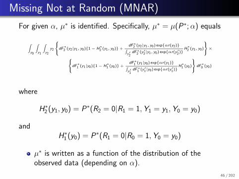
Missing Not at Random (MNAR)
For given α, µ∗ is identified. Specifically, µ∗ = µ(P∗;α) equals
∫y0
∫y1
∫y2
y2
dF∗2 (y2|y1, y0){1− H∗2 (y1, y0)} +dF∗2 (y2|y1, y0) exp{αr(y2)}∫y′2dF∗2 (y′2 |y1, y0) exp{αr(y
′2)}
H∗2 (y1, y0)
×dF∗1 (y1|y0){1− H∗1 (y0)} +dF∗1 (y1|y0) exp{αr(y1)}∫y′1dF∗1 (y′1 |y0) exp{αr(y
′1)}
H∗1 (y0)
dF∗0 (y0)
where
H∗2 (y1, y0) = P∗(R2 = 0|R1 = 1,Y1 = y1,Y0 = y0)
andH∗1 (y0) = P∗(R1 = 0|R0 = 1,Y0 = y0)
µ∗ is written as a function of the distribution of theobserved data (depending on α).
46 / 202

Global Sensitivity Analysis
1
I
YH Jul 16
Y0 Y1 Y2
A0(y
0)
B1(y
0)
II
Y0 Y1 Y2
f∗(Y1|A0(y0)) ∝f∗(Y1|B1(y0))e
αr(Y1)
Low High
Assumption
MAR (α = 0)
MNAR (α < 0)
MNAR (α > 0)
A0(y
0)
B1(y
0)
III
Y0 Y1 Y2
47 / 202

Global Sensitivity Analysis
1
A0(y
0)
B1(y
0)
III
Y0 Y1 Y2
f∗(Y2|A1(y0, y1)) ∝f∗(Y2|B2(y0, y1))e
αr(Y2)
for all y0, y1
Example for y0, y1
A1(y
0,y
1)
B2(y
0,y
1)
IV V
Y0 Y1 Y2 Y0 Y1 Y2
YH Jul 16
Low High
Assumption
MAR (α = 0)
MNAR (α < 0)
MNAR (α > 0)
A0(y
0)
B1(y
0)
V I
Y0 Y1 Y2
48 / 202

Global Sensitivity Analysis
1
A0(y
0)
B1(y
0)
V I
Y0 Y1 Y2f∗(Y2|A0(y0), Y1 = y1) =
f∗(Y2|B1(y0), Y1 = y1)
for all y0, y1
Example for y0, y1
Y1=
y1
A0(y
0)
Y1=
y1
B1(y
0)
V II V III
Y0 Y1 Y2 Y0 Y1 Y2
YH Jul 16
Low High
A0(y
0)
B1(y
0)
IX
Y0 Y1 Y2
49 / 202

Inference
For given α, the above formula shows that µ∗ depends on
F ∗2 (y2|y1, y0) = P∗(Y2 ≤ y2|B2(y1, y0))
F ∗1 (y1|y0) = P∗(Y1 ≤ y1|B1(y0))
H∗2 (y1, y0) = P∗(R2 = 0|R1 = 1,Y1 = y1,Y0 = y0)
H∗1 (y0) = P∗(R1 = 0|R0 = 1,Y0 = y0).
It is natural to consider estimating µ∗ by “plugging in”estimators of these quantities.
How can we estimate these latter quantities? With theexception of F ∗0 (y0), it is tempting to think that we can usenon-parametric procedures to estimate these quantities.
50 / 202

Inference
A non-parametric estimate of F ∗2 (y2|y1, y0) would take theform:
F2(y2|y1, y0) =
∑ni=1 R2,i I (Y2,i ≤ y2)I (Y1,i = y1,Y0,i = y0)∑n
i=1 R2,i I (Y1,i = y1,Y0,i = y0)
This estimator will perform very poorly (i.e., have highlevels of uncertainty in moderate sample sizes) becausethe number of subjects who complete the study (i.e.,R2 = 1) and are observed to have outcomes at visits 1and 0 exactly equal to y1 and y0 will be very small andcan only be expected to grow very slowly as the samplesize increases.
As a result, a a plug-in estimator of µ∗ that uses suchnon-parametric estimators will perform poorly.
51 / 202

Inference - Type (ii) Assumptions
We make the estimation task slightly easier by assuming that
F ∗2 (y2|y1, y0) = F ∗2 (y2|y1) (7)
andH∗2 (y1, y0) = H∗2 (y1) (8)
52 / 202

Inference - Kernel Smoothing
Estimate F ∗2 (y2|y1), F ∗1 (y1|y0), H∗2 (y1) and H∗1 (y0) using kernelsmoothing techniques.
To motivate this idea, consider the following non-parametricestimate of F ∗2 (y2|y1)
F2(y2|y1) =
∑ni=1 R2,i I (Y2,i ≤ y2)I (Y1,i = y1)∑n
i=1 R2,i I (Y1,i = y1)
This estimator will still perform poorly, although betterthan F2(y2|y1, y0).
Replace I (Y1,i = y1) by φ(
Y1,i−y1σF2
), where φ(·) is
standard normal density and σF2 is a tuning parameter.
F2(y2|y1;σF2) =
∑ni=1 R2,i I (Y2,i ≤ y2)φ
(Y1,i−y1σF2
)∑n
i=1 R2,iφ(
Y1,i−y1σF2
)53 / 202

Inference - Kernel Smoothing
This estimator allows all completers to contribute, notjust those with Y1 values equal to y1
It assigns weight to completers according to how far theirY1 values are from y1, with closer values assigned moreweight.
The larger σF2 , the larger the influence of values of Y1
further from y1 on the estimator.
As σF2 →∞, the contribution of each completer to theestimator becomes equal, yielding bias but low variance.
As σF2 → 0, only completers with Y1 values equal to y1contribute, yielding low bias but high variance.
54 / 202

Inference - Cross-Validation
To address the bias-variance trade-off, cross validation istypically used to select σF2 .
Randomly divide dataset into J (typically, 10)approximately equal sized validation sets.Let Vj be the indices of the patients in jth validation set.Let nj be the associated number of subjects.
Let F(j)2 (y2|y1;σF2) be the estimator of F ∗2 (y2|y1) based
on the dataset that excludes the jth validation set.If σF2 is a good choice then one would expect
CVF∗2(·|·)(σF2 ) =
1
J
J∑j=1
1
nj
∑i∈Vj
R2,i
∫ {I (Y2,i ≤ y2)− F
(j)2 (y2|Y1,i ;σF2 )
}2dF◦2 (y2)︸ ︷︷ ︸
Distance for i ∈ Vj
will be small, where F ◦2 (y2) is the empirical distribution ofY2 among subjects on-study at visit 2.
55 / 202

Inference - Cross-Validation
For each individual i in the jth validation set with anobserved outcome at visit 2, we measure, by the quantityabove the horizontal brace, the distance (or loss) betweenthe collection of indicator variables{I (Y2,i ≤ y2) : dF ◦2 (y2) > 0} and the correspondingcollection of predicted values{F (j)
2 (y2|Y1,i ;σF2) : dF ◦2 (y2) > 0}.The distances for each of these individuals are thensummed and divided by the number of subjects in the jthvalidation set.
An average across the J validation/training sets iscomputed.
We can then estimate F ∗2 (y2|y1) by F2(y2|y1; σF2), whereσF2 = argmin CVF∗2 (·|·)(σF2).
56 / 202

Inference - Cross-Validation
We use similar ideas to estimate
F ∗1 (y1|y0)
H∗2 (y1)
H∗1 (y0)
In our software, we set σF2 = σF1 = σF and minimize a singleCV function. The software refers to this smoothing parameteras σQ .
In our software, we set σH2 = σH1 = σH and minimize a singleCV function. The software refers to this smoothing parameteras σP .
57 / 202

Inference - Potential Problem
The cross-validation procedure for selecting tuningparameters achieves optimal finite-sample bias-variancetrade-off for the quantities requiring smoothing.
This optimal trade-off is usually not optimal forestimating µ∗.
The plug-in estimator of µ∗ could possibly suffer fromexcessive and asymptotically non-negligible bias due toinadequate tuning.
This may prevent the plug-in estimator from havingregular asymptotic behavior, upon which statisticalinference is generally based.
The resulting estimator may have a slow rate ofconvergence, and common methods for constructingconfidence intervals, such as the Wald and bootstrapintervals, can have poor coverage properties.
58 / 202

Inference - Correction Procedure
Let M be the class of distributions for the observed dataO that satisfy constraints (7) and (8).
For P ∈M, it can be shown that
µ(P ;α)− µ(P∗;α)
= −E ∗[ψP(O;α)− ψP∗(O;α)] + Rem(P ,P∗;α), (9)
where ψP(O;α) is a “derivative” of µ(·;α) at P andRem(P ,P∗;α) is a ”second-order” remainder term whichconverges to zero as P tends to P∗.The derivative is used to quantify the change in µ(P ;α)resulting from small perturbations in P ; it also has meanzero (i.e., E ∗[ψP∗(O;α)] = 0).
The remainder term is second order in the sense that itcan be written as or bounded by the product of termsinvolving differences between (functionals of) P and P∗.
59 / 202

Inference - Correction Procedure
Equation (9) plus some simple algebraic manipulation teachesus that
µ(P ;α)︸ ︷︷ ︸Plug-in
−µ(P∗;α)
=1
n
n∑i=1
ψP∗(Oi ;α)− 1
n
n∑i=1
ψP(Oi ;α) (10)
+1
n
n∑i=1
{ψP(Oi ;α)− ψP∗(Oi ;α)− E ∗[ψP(O;α)− ψP∗(O;α)]}
(11)
+ Rem(P ,P∗;α) (12)
where P is the estimated distribution of P∗ discussed in theprevious section.
60 / 202

Inference - Correction Procedure
Under smoothness and boundedness conditions, term (11)will be oP∗(n
−1/2) (i.e., will converge in probabity to zeroeven when it is multipled by
√n).
Provided P converges to P∗ at a reasonably fast rate,term (12) will also be oP∗(n
−1/2).
The second term in (10) prevents us from concluding thatthe plug-in estimator can be essentially represented as anaverage of i.i.d terms plus oP∗(n
−1/2) terms.
By adding the second term in (10) to the plug-inestimator, we can construct a “corrected” estimator thatdoes have this representation.
61 / 202

Inference - Correction Procedure
The corrected estimator is
µα = µ(P ;α)︸ ︷︷ ︸Plug-in
+1
n
n∑i=1
ψP(Oi ;α)
The practical implication is that µα converges in probability toµ∗ and
√n (µα − µ∗) =
1√n
n∑i=1
ψP∗(Oi ;α) + oP∗(1)
With this representation, we see that ψP∗(O;α) is theso-called influence function.
62 / 202

Inference - Correction Procedure
By the central limit theorem, we then know that√n (µα − µ∗) converges to a normal random variable
with mean 0 and variance σ2α = E ∗[ψP∗(O;α)2].
The asymptotic variance can be estimated byσ2α = 1
n
∑ni=1 ψP(Oi ;α)2.
A (1− γ)% Wald-based confidence interval for µ∗ can beconstructed as µα ± z1−γ/2σα/
√n, where zq is the qth
quantile of a standard normal random variable.
63 / 202

Inference - Efficient Influence Function/Gradient
Let
π∗(y0, y1, y2;α)−1 = (1 + exp{l∗1 (y0;α) + αr(y1)})×(1 + exp{l∗2 (y1;α) + αr(y2)})
w ∗1 (y0;α) = E ∗ [exp{αr(Y1)} | R1 = 1,Y0 = y0] ,
w ∗2 (y1;α) = E ∗ [exp{αr(Y2)} | R2 = 1,Y1 = y1] ,
g ∗1 (y0, y1;α) = {1− H∗1 (y0)}w ∗1 (y0;α) + exp{αr(y1)}H∗1 (y0).
g ∗2 (y1, y2;α) = {1− H∗2 (y1)}w ∗2 (y1;α) + exp{αr(y2)}H∗2 (y1).
64 / 202

Inference - Efficient Influence Function/Gradient
ψP∗(O;α) := a∗0(Y0;α) +
R1b∗1(Y0,Y1;α) +
R2b∗2(Y1,Y2;α) +
{1− R1 − H∗1 (Y0)}c∗1 (Y0;α) +
R1{1− R2 − H∗2 (Y1)}c∗2 (Y1;α)
where
65 / 202

Inference - Efficient Influence Function/Gradient
a∗0 (Y0) = E∗[
R2Y2
π∗(Y0, Y1, Y2;α)Y0
]− µ(P∗;α)
b∗1 (Y0, Y1;α) = E∗[
R2Y2
π∗(Y0, Y1, Y2;α)R1 = 1, Y1, Y0
]− E∗
[R2Y2
π∗(Y0, Y1, Y2;α)R1 = 1, Y0
]
+ E∗[
R2Y2
π∗(Y0, Y1, Y2;α)
[exp{αr(Y1)}g∗1 (Y0, Y1;α)
]R1 = 1, Y0
]H∗1 (Y0)
{1−
exp{αr(Y1)}w∗1 (Y0;α)
}
b∗2 (Y1, Y2;α) = E∗[
R2Y2
π∗(Y0, Y1, Y2;α)R2 = 1, Y2, Y1
]− E∗
[R2Y2
π∗(Y0, Y1, Y2;α)R2 = 1, Y1
]
+ E∗[
R2Y2
π∗(Y0, Y1, Y2;α)
[exp{αr(Y2)}g∗2 (Y1, Y2;α)
]R2 = 1, Y1
]H∗2 (Y1)
{1−
exp{αr(Y2)}w∗2 (Y1;α)
}
c∗1 (Y0) = E∗[
R2Y2
π∗(Y0, Y1, Y2;α)
[exp{αr(Y1)}g∗1 (Y0, Y1;α)
]Y0
]
− E∗[
R2Y2
π∗(Y0, Y1, Y2;α)
[1
g∗1 (Y0, Y1;α)
]Y0
]w∗1 (Y0;α)
c∗2 (Y1) = E∗[
R2Y2
π∗(Y0, Y1, Y2;α)
[exp{αr(Y2)}g∗2 (Y1, Y2;α)
]R1 = 1, Y1
]
− E∗[
R2Y2
π∗(Y0, Y1, Y2;α)
[1
g∗2 (Y1, Y2;α)
]R1 = 1, Y1
]w∗2 (Y1;α)
66 / 202

Inference - Uncertainty
Wald-based confidence intervals don’t always haveadequate coverage properties is finite samples.
In equal-tailed studentized bootstrap, the confidenceinterval takes the form [µ− t0.975se(µ), µ− t0.025se(µ)],
where tq is the qth quantile of{µ(b)−µse(µ(b))
: b = 1, . . . ,B}
In symmetric studentized bootstrap, the confidenceinterval takes the form [µ− t∗0.95se(µ), µ + t∗0.95se(µ)],where t∗0.95 is selected so that 95% of the distribution of{µ(b)−µse(µ(b))
: b = 1, . . . ,B}
falls between −t∗0.95 and t∗0.95.
Useful to replace influence-function based standard errorestimator with jackknife standard error estimator.
67 / 202

Quetiapine Bipolar Trial - Fit
Estimated smoothing parameters for the drop-out modelare 11.54 and 9.82 for the placebo and 600 mg arms.
Estimated smoothing parameters for the outcome modelare 6.34 and 8.05 for the placebo and 600 mg arms.
In the placebo arm, the observed percentages of lastbeing seen at visits 0 and 1 among those at risk at thesevisits are 8.62% and 38.68%. Model-based estimates are7.99% and 38.19%.
For the 600 mg arm, the observed percentages are11.02% and 35.24% and the model-based estimates are11.70% and 35.08%.
68 / 202

Quetiapine Bipolar Trial - Fit
In the placebo arm, the Kolmogorov-Smirnov distancesbetween the empirical distribution of the observedoutcomes and the model-based estimates of thedistribution of outcomes among those on-study at visits 1and 2 are 0.013 and 0.033.
In the 600 mg arm, these distances are 0.013 and 0.022.
These results suggest that our model for the observeddata fits the observed data well.
69 / 202

Quetiapine Bipolar Trial - MAR
Under MAR, the estimated values of µ∗ are 46.45 (95%CI: 42.35,50.54) and 62.87 (95% CI: 58.60,67.14) for theplacebo and 600 mg arms.
The estimated difference between 600 mg and placebo is16.42 (95% 10.34, 22.51)
Statistically and clinically significant improvement inquality of life in favor of Quetiapine.
70 / 202

Quetiapine Bipolar Trial - Sensitivity Analysis
We set r(y) = y and ranged the sensitivity analysisparameter from -10 and 10 in each treatment arm.
According to experts, there is no evidence to suggest thatthere is a differential effect of a unit change in QLESSFon the hazard of drop-out based on its location on thescale.
71 / 202

Quetiapine Bipolar Trial - Sensitivity Analysis
Figure: Treatment-specific (left: placebo; right: 600 mg/dayQuetiapine) estimates (along with 95% pointwise confidenceintervals) of µ∗ as a function of α.
−10 −5 0 5 10
4050
6070
80
α
Est
imat
e
−10 −5 0 5 10
4050
6070
80
α
Est
imat
e
72 / 202

Quetiapine Bipolar Trial - Sensitivity Analysis
Figure: Treatment-specific differences between the estimated meanQLESSF at Visit 2 among non-completers and the estimated meanamong completers, as a function of α.
PlaceboQuetiapine (600mg)
−10 −5 0 5 10
−20
−15
−10
−5
05
10
α
Diff
eren
ce in
Mea
n Q
LES
SF
(Non
−co
mpl
eter
s m
inus
Com
plet
ers)
73 / 202

Quetiapine Bipolar Trial - Sensitivity Analysis
Figure: Contour plot of the estimated differences between meanQLESSF at Visit 2 for Quetiapine vs. placebo for varioustreatment-specific combinations of the sensitivity analysisparameters.
0
5
10
15
20
25
30
−10 −5 0 5 10
−10
−5
0
5
10
α (Placebo)
α (Q
uetia
pine
600
mg)
74 / 202

Quetiapine Bipolar Trial - Sensitivity Analysis
Only when the sensitivity analysis are highly differential(e.g., α(placebo) = 8 and α(Quetiapine) = −8) are thedifferences no longer statistically significant.
75 / 202

Quetiapine Bipolar Trial - Sensitivity Analysis
0 20 40 60 80 100
QLESSF at time 0
0
20
40
60
80
100
Mea
n Q
LES
SF
at t
ime
1
OtherAdverse event
α = -10α = -5
α = -1α = 1
α = 5
α = 10
α = 0
0 20 40 60 80 100
QLESSF at time 1
0
20
40
60
80
100
Mea
n Q
LES
SF
at t
ime
2
OtherLack of efficacyAdverse event
α = -10α = -5
α = -1α = 1
α = 5
α = 10
α = 0
76 / 202

Quetiapine Bipolar Trial - Sensitivity Analysis
0 20 40 60 80 100
QLESSF at time 0
0
20
40
60
80
100
Mea
n Q
LES
SF
at t
ime
1
OtherAdverse event
α = -10
α = -5
α = -1
α = 1
α = 5
α = 10
α = 0
0 20 40 60 80 100
QLESSF at time 1
0
20
40
60
80
100
Mea
n Q
LES
SF
at t
ime
2
OtherAdverse event
α = -10α = -5
α = -1
α = 1α = 5
α = 10
α = 0
77 / 202

Quetiapine Bipolar Trial - Sensitivity Analysis
Conclusions under MAR are highly robust.
78 / 202

Simulation Study
Generated 2500 placebo and Quetiapine datasets usingthe estimated distributions of the observed data from theQuentiapine study as the true data generatingmechanisms.
For given treatment-specific α, these true data generatingmechanisms can be mapped to a true value of µ∗.
For each dataset, the sample size was to set to 116 and118 in the placebo and Quetiapine arms, respectively.
79 / 202

Simulation Study - Bias/MSE
Placebo Quetiapineα Estimator µ∗ Bias MSE µ∗ Bias MSE
-10 Plug-in 40.85 0.02 4.43 56.07 0.40 4.69Corrected 0.43 4.56 0.42 4.72
-5 Plug-in 43.45 0.05 4.29 59.29 0.34 4.55Corrected 0.27 4.26 0.24 4.35
-1 Plug-in 46.02 0.28 4.34 62.58 0.50 4.39Corrected 0.18 4.22 0.14 4.00
0 Plug-in 46.73 0.36 4.44 63.42 0.55 4.36Corrected 0.17 4.27 0.14 3.95
1 Plug-in 47.45 0.43 4.57 64.25 0.59 4.32Corrected 0.16 4.36 0.15 3.92
5 Plug-in 50.48 0.66 5.33 67.34 0.59 4.20Corrected 0.14 5.11 0.19 4.15
10 Plug-in 54.07 0.51 5.78 70.51 0.07 4.02Corrected 0.04 6.30 -0.05 4.66
80 / 202

Simulation Study - Coverage
Placebo Quetiapineα Procedure Coverage Coverage-10 Wald-IF 91.5% 90.5%
Wald-JK 95.0% 94.6%Bootstrap-IF-ET 94.3% 93.8%Bootstap-JK-ET 94.4% 93.4%Bootstap-IF-S 95.2% 94.6%Bootstap-JK-S 95.0% 94.6%
-5 Wald-IF 93.5% 92.9%Wald-JK 95.0% 94.8%Bootstrap-IF-ET 95.2% 94.6%Bootstap-JK-ET 94.8% 94.6%Bootstap-IF-S 95.4% 95.2%Bootstap-JK-S 95.1% 95.2%
-1 Wald-IF 93.9% 94.2%Wald-JK 94.9% 95.4%Bootstrap-IF-ET 95.1% 94.8%Bootstap-JK-ET 95.1% 94.6%Bootstap-IF-S 95.3% 96.4%Bootstap-JK-S 95.1% 96.3%
0 Wald-IF 93.8% 94.0%Wald-JK 95.0% 95.4%Bootstrap-IF-ET 94.6% 94.5%Bootstap-JK-ET 94.6% 94.6%Bootstap-IF-S 95.5% 96.6%Bootstap-JK-S 95.2% 96.7%
81 / 202

Simulation Study - Coverage
Placebo Quetiapineα Procedure Coverage Coverage1 Wald-IF 93.3% 93.7%
Wald-JK 95.1% 95.5%Bootstrap-IF-ET 94.6% 94.6%Bootstap-JK-ET 94.6% 94.6%Bootstap-IF-S 95.5% 96.5%Bootstap-JK-S 95.2% 96.5%
5 Wald-IF 90.8% 91.3%Wald-JK 95.3% 95.7%Bootstrap-IF-ET 93.2% 91.6%Bootstap-JK-ET 93.8% 93.0%Bootstap-IF-S 95.5% 95.4%Bootstap-JK-S 95.8% 96.4%
10 Wald-IF 85.4% 87.8%Wald-JK 94.9% 94.5%Bootstrap-IF-ET 88.2% 87.0%Bootstap-JK-ET 92.2% 89.7%Bootstap-IF-S 94.6% 93.9%Bootstap-JK-S 95.5% 95.1%
82 / 202

Software
1. R
samon libraryfunctions with pass to C code
2. SAS
procedures and macros
83 / 202

The Quet1/Quet2 Dataset
proc print data = quet1;
run;
Obs V1 V2 V3
1 36 56 57
2 32 32 31
3 25 42 27
4 48 52 54
5 27 40 40
6 38 43 .
7 35 44 39
8 24 26 28
9 25 30 .
10 25 28 .
11 40 45 45
12 14 16 .
13 34 37 .
14 27 25 .
15 26 25 .
16 38 . .
17 44 . .
18 35 31 .
19 25 45 49
20 45 53 56
21 32 38 48
22 46 45 .
23 30 . .
24 43 56 43
25 42 44 41
26 34 45 47
27 34 . .
84 / 202

SAS: samonDataCheck macro
samonDataCheck macro can be used to check themissing data pattern in the data.
%samonDataCheck(data = input datasetvars = variable list (in time order)out = output datastats = output statistics datasetmpattern = missing pattern counts dataset);
85 / 202

SAS: samonDataCheck macro
%samonDataCheck(
data = quet1,
vars = v1 v2 v3,
out = check1,
stats = stats1t,
mpattern = pattern1);
86 / 202

R: samonDataCheck function
In R, the samonDataCheck function can be used for thesame purpose:
samonDataCheck( quet1 )
> # R version of samonDataCheck is a
> # function of the same name
>
> # Check data
> chk1 <- samonDataCheck( quet1 )
>
> chk2 <- samonDataCheck( quet2 )
87 / 202

samonDataCheck
Samon Data Check:
-----------------------------------------------
Number of time-points: 3
Number of subjects: 116
Minimum observed value: 14
Maximum observed value: 63
Average number of timepoints on study: 2.47
Total number of observed values: 287
Subjects observed at final timepoint: 65
Subjects observed at all timepoint: 65
Missing Patterns:
N proportion
*__ : 10 0.0862
**_ : 41 0.3534
*** : 65 0.560388 / 202

samonDataCheck
Samon Data Check:
-----------------------------------------------
Number of time-points: 3
Number of subjects: 118
Minimum observed value: 15
Maximum observed value: 67
Average number of timepoints on study: 2.47
Total number of observed values: 291
Subjects observed at final timepoint: 68
Subjects observed at all timepoint: 68
Missing Patterns:
N proportion
*__ : 13 0.1102
**_ : 37 0.3136
*** : 68 0.576389 / 202

10 20 30 40 50 60 70
Observed Score
0
10
200.0
0.2
0.4
0.6
0.8
1.0D
ropo
ut R
ate
90 / 202

10 20 30 40 50 60 70
Observed Score
0
10
200.0
0.2
0.4
0.6
0.8
1.0D
ropo
ut R
ate
91 / 202

10 20 30 40 50 60 70
Observed Score
0
10
200.0
0.2
0.4
0.6
0.8
1.0D
ropo
ut R
ate
σ = 1
σ = 3
σ = 5
σ = 10
92 / 202

10 20 30 40 50 60 70
Observed Score
0
10
200.0
0.2
0.4
0.6
0.8
1.0D
ropo
ut R
ate
σ = 1
σ = 2
σ = 5
σ = 10
93 / 202

R: samoneval function
samoneval function can be used to compute the lossfunction for a range of σ.
Takes four arguments:
samoneval(
mat = , # input matrix to evaluate
Npart = 10, # number of partitions
sigmaList = c(0,1), # vector of sigma values
type = ”both” # compute the loss function for σH ,σF , or both σH and σF
)
Returns a matrix containing σH and its corresponding lossfunction value and σF and its corresponding loss functionvalue.
94 / 202

R: samoneval function
> library(samon, lib.loc="../samlib")
>
> Results1 <- samoneval(
+ mat = quet1,
+ Npart = 10,
+ sigmaList = seq(0.2,30.0,by=0.1),
+ type = "both"
+ )
95 / 202

R: samoneval function
> Results2 <- samoneval(
+ mat = quet2,
+ Npart = 10,
+ sigmaList = seq(0.2,30.0,by=0.1),
+ type = "both"
+ )
> ResultsH <- cbind(Results1[,1:2],
+ Results2[,1:2])
> HFPlot(ResultsH, "H.pdf", 4.2, 4.2,
+ "Loss function (H)", c(0,30),
+ c( 2.5, 4.5), c(15,4.5) )
96 / 202

samonev procedure
The samonev procedure computes the loss function for arange of σ.samonev
data = Input dataset
out = Output dataset
npart = Number of partitions
var varlist list of variables in time order
sigma sigmalist list of sigmas
97 / 202

samonev procedure
proc samonev
data = quet1
out = ev1
Npart = 10;
var v1 - v3;
sigma 0.2 to 30 by 0.1;
run;
98 / 202

0 5 10 15 20 25 30
2.5
3.0
3.5
4.0
4.5
Treatment 1Treatment 2
σ
Loss
Fun
ctio
n (H
)
99 / 202

0 5 10 15 20 25 30
1.5
2.0
2.5
3.0
3.5
4.0
Treatment 1Treatment 2
σ
Loss
Fun
ctio
n (F
)
100 / 202

samon
The samon function and the samon procedure can be used tofind optimal values of σH and σF . Like many optimizationtechniques providing good initial estimates can improve theefficiency of convergence of the optimization. Within samon
we also provide an upper bound for σH and σF . Should thealgorithm begin to converge to an optimal value greater thanthe upper bound, samon returns the upper bound itself ratherthan search for an optimal value above this upper bound. Thisis to reflect the fact that larger values of σH or σF result inlittle change in the smoothing.
101 / 202

R: samon function
# Example1.R# Finding optimal Sigma_h and Sigma_f.# ----------------------------------------library(samon, lib.loc="../samlib")
samonResults <- samon(mat = quet1,Npart = 10,
InitialSigmaH = 6.0,HighSigmaH = 50.0,
InitialSigmaF = 4.0,HighSigmaF = 50.0
)
# print the outputprint(samonResults)
102 / 202

SAS: samon procedure
* Finding optimal Sigma_h and Sigma_f.;* ----------------------------------------;proc samon data = quet1
out = samon1Npart = 10Hinit = 6.0Hhigh = 50.0Finit = 4.0Fhigh = 50Hout = HM1Fout = FM1;
var v1 - v3;run;
103 / 202

Treatment 1
proc print data = HM1 noobs;run;
rc Niter Sigma loss2 3 6.6918 2.7468
proc print data = FM1 noobs;run;
rc Niter Sigma loss2 6 3.6771 1.9057
104 / 202

Treatment 2
proc print data = HM2 noobs;run;
rc Niter Sigma loss2 3 5.6938 2.9607
proc print data = FM2 noobs;run;
rc Niter Sigma loss2 3 4.6704 2.1872
105 / 202

Sensitivity Analysis
Within samon the sensitivity bias function is thecumulative function of the beta distribution, a flexiblefunction with bounded support.
This together with the sensitivity analysis parameter αprovides the mechanism by which we measure thesensitivity of the results to informative drop-out.
106 / 202

Sensitivity Analysis
The cumulative beta function is defined on the interval(0,1) and in order to use it as the sensitivity bias functionwe need to map the range of our data into (0,1).
In the case of QLESSF scores the data are limited to therange 13 and 71.
We take the parameters for the cumulative beta functionζ1 and ζ2 to be 1.
107 / 202

20 40 60
QLESSF
0.0
0.2
0.4
0.6
0.8
1.0(ζ1, ζ2) = (1,4)
(ζ1, ζ2) = (1,1)
(ζ1, ζ2) = (8,2)
108 / 202

samon proceduresamon
data = Input datasetIFout = Influence function estimatesnpart = Number of partitionsHinit = initial value for smoothing parameter sigma HHhigh = Highest value for smoothing parameter sigma HFinit = initial value for smoothing parameter sigma FFhigh = Highest value for smoothing parameter sigma Flb = lower bound of dataub = upper bound of datazeta1 = parameter for cumulative beta distributionzeta2 = parameter for cumulative beta distributionnsamples = Number of bootstrap samplesseed0 = Seed to pass to random number generator
var varlist list of variables in time ordersensp senslist list of sensitivity parameters
109 / 202

proc samon data = quet1 IFout = IFM1Npart = 10Hinit = 6.0 HHigh = 50.0Finit = 4.0 FHigh = 50.0
lb = 13 ub = 71zeta1 = 1.0 zeta2 = 1.0nomj nsamples = 0 ;
var v1 - v3;sensp -10 to 10 by 1;
run;proc print data = IFM1 noobs;var alpha AEst AVar IFEst IFVar;
run;
110 / 202

# Produce one-step influence function estimates# ----------------------------------------------library(samon, lib.loc="../samlib")
Results1 <- samon(mat = quet1,Npart = 10,
# initial value and upper bound for sigmaHInitialSigmaH = 6.0,HighSigmaH = 50.0,
# initial value and upper bound for sigmaFInitialSigmaF = 4.0,HighSigmaF = 50.0,
AlphaList = -10:10, # alphas
lb = 13, ub = 71,zeta1 = 1.0, zeta2 = 1.0
111 / 202

alpha AEst AVar IFEst IFVar
-10 36.6909 0.08754 36.9454 1.3374
-9 36.9556 0.09050 37.2108 1.3438
-8 37.2402 0.09354 37.4881 1.3497
-7 37.5435 0.09653 37.7740 1.3547
-6 37.8641 0.09934 38.0654 1.3585
-5 38.2007 0.10185 38.3611 1.3609
-4 38.5526 0.10395 38.6609 1.3625
-3 38.9189 0.10556 38.9660 1.3641
-2 39.2993 0.10660 39.2787 1.3668
-1 39.6935 0.10701 39.6020 1.3715
0 40.1010 0.10678 39.9386 1.3792
1 40.5210 0.10590 40.2911 1.3898
2 40.9517 0.10436 40.6609 1.4026
3 41.3907 0.10222 41.0484 1.4160
4 41.8343 0.09950 41.4525 1.4278
5 42.2785 0.09626 41.8710 1.4356
6 42.7186 0.09252 42.3006 1.4374
7 43.1501 0.08832 42.7372 1.4320
8 43.5690 0.08370 43.1760 1.4190
9 43.9724 0.07871 43.6127 1.3989
10 44.3586 0.07345 44.0435 1.3729
112 / 202

−10 −5 0 5 10
3035
4045
5055
60
α
QLE
SS
F E
stim
ate
at V
isit
2
113 / 202

Confidence intervals
Use bootstrap with jackknife to compute confidenceintervals.
The NSamples argument controls the number ofbootstraps to make.
The flags mj and sj control whether jackknifes areperformed on the main (input) data and the bootstrapsamples respectively.
For a small dataset with 100 individuals, 1,000 bootstrapseach with bootstrap estimates on 50 sensitivityparameters gives rise to 50 x 100 x 1000 = 5 millionestimates.
114 / 202

proc samon data = quet1 out = samon1
Npart = 10
Hinit = 6.0 HHigh = 50.0
FInit = 4.0 FHigh = 50.0
lb = 13 ub = 71
zeta1 = 1.0 zeta2 = 1.0
NSamples = 500 seed0 = 81881
sj;
var v1-v3;
sensp -10 to 10 by 1;
run;
115 / 202

%samonSummary(
data = results1,
out = data.Summary1,
sampout = data.sampSummary1
);
proc print data=data.Summary1;
var alpha IFEst lb ub;
run;
116 / 202

alpha IFEst lb ub
-10 36.9454 34.2645 39.6263
-9 37.2108 34.5635 39.8580
-8 37.4881 34.9005 40.0757
-7 37.7740 35.2496 40.2984
-6 38.0654 35.5840 40.5468
-5 38.3611 35.9267 40.7955
-4 38.6609 36.2627 41.0590
-3 38.9660 36.6038 41.3281
-2 39.2787 36.9218 41.6356
-1 39.6020 37.2546 41.9493
0 39.9386 37.5628 42.3144
1 40.2911 37.8957 42.6866
2 40.6609 38.2211 43.1007
3 41.0484 38.5820 43.5148
4 41.4525 38.9005 44.0045
5 41.8710 39.2378 44.5043
6 42.3006 39.5695 45.0318
7 42.7372 39.9254 45.5490
8 43.1760 40.2880 46.0641
9 43.6127 40.5862 46.6392
10 44.0435 40.8705 47.2165
117 / 202

We use the samonCrossSummary function to compute thedifference in estimates for each pair of alpha.
118 / 202

%samonCrossSummary(
IFM1 = data.Summary1,
sampIF1 = data.sampSummary1,
IFM2 = data.Summary2,
sampIF2 = data.sampSummary2,
out = data.Cross
);
119 / 202

macro description
samonCombine Combines results from multiple runs of procsamon
samonSummary Summarizes samon results. Combines boot-strap and jackknife results to produce con-fidence intervals
samonDifferenceSummary Computes treatment effect differencesand confidence intervals from a pair ofsamonSummary objects.
samonCrossSummary Computes treatment effect differences andconfidence intervals for each pair of sensi-tivity parameters α.
samonECompleterStatus Computes the difference in the expectedvalue of non-completers and completers
120 / 202

samonCombine macrosamonCombine combines samon results into one dataset
(
inlib = input libref
stem = results file name stem
connect = name connector
partfrom = 1 parts start at 1
partto = 100 to 100
partform = z5 format to use on partno
outlib = output libref
)
121 / 202

samonSummary macrosamonSummary computes summary of samon object
(
data = input dataset to summarize
out = summary of main data
sampSummary = summary of parametric bootstrap samples
)
122 / 202

samonDifferenceSummary macrosamonDifferenceSummary Treatment-specific differences
(
IFM1 = main results from samonSummary for trt 1
sampIF1 = sample results from samonSummary for trt 1
IFM2 = main results from samonSummary for trt 2
sampIF2 = sample results from samonSummary for trt 2
out = summary of difference
)
123 / 202

samonCrossSummary macrosamonCrossSummary Treatment-specific differences for all pairs of
sensitivity parameter
(
IFM1 = main results from samonSummary for trt 1
sampIF1 = sample results from samonSummary for trt 1
IFM2 = main results from samonSummary for trt 2
sampIF2 = sample results from samonSummary for trt 2
out = summary of difference
)
124 / 202

R: samon function
function descriptionsamonCombine combines the outputs from samon into one
samonMat object. The results are stored as.Rds files. samonCombine takes a list of suchfilesand combines them.
samonDiff Takes two samonMat objects and produces asamonMat object for the difference ininfluence function estimates
samonBiasCorrection Takes a samonMat object and produces cor-rected influence function estimates
samonXBiasCorrection Takes two samonMat objects (one from eachtreatment groups) and for each pair of alphasproduces the difference in influence function es-timates.
125 / 202

Generalization
Yk : outcome scheduled to be measured at assessment k .
Rk : indicator that individual is on-study at assessment k .
All individuals are present at baseline, i.e., R0 = 1.
Monotone missing data: Rk+1 = 1 implies Rk = 1.
C = max{k : Rk = 1}, C = K implies that the individualcompleted the study.
For any given vector z = (z1, z2, . . . , zK ),
zk = (z0, z1, . . . , zk)zk = (zk+1, zk+2, . . . , zK ).
For each individual, the data unit O = (C ,Y C ) is drawnfrom some distribution P∗ contained in thenon-parametric model M of distributions.
The observed data consist of n independent drawsO1,O2, . . . ,On from P∗.
126 / 202

Generalization
By factorizing the distribution of O in terms of chronologicallyordered conditional distributions, any distribution P ∈M canbe represented by
F0(y0) := P (Y0 ≤ y0);
Fk+1(yk+1 | y k) :=P(Yk+1 ≤ yk+1 | Rk+1 = 1,Y k = y k
),
k = 0, 1, . . . ,K − 1;
Hk+1(yk) := P(Rk+1 = 0 | Rk = 1,Y k = y k
),
k = 0, 1, . . . ,K − 1.
The main objective is to draw inference about µ∗ := E ∗(YK ),the true mean outcome at visit K in a hypothetical world inwhich all patients are followed to that visit.
127 / 202

Missing at Random
For every y k , define the following strata:
Ak(y k): patients last seen at visit k (i.e.,Rk = 1,Rk+1 = 0) with Y k = y k .
Bk+1(y k): patients on-study at visit k + 1 (i.e.,Rk+1 = 1) with Y k = y k .
128 / 202

Missing at Random
For all y k , the distribution of Y k for patients instratum Ak(y k) is the same as the distribution of Y k
for patients in stratum Bk+1(y k)
Mathematically, we can express these assumptions as follows:
f ∗(Y k |Ak(y k)) = f ∗(Y k |Bk+1(y k)) for all y k (13)
129 / 202

Missing at Random
Using Bayes’ rule, we can re-write these expressions as:
P∗(Rk+1 = 0|Rk = 1,Y K = yK )
= P∗(Rk+1 = 0|Rk = 1,Y k = y k) for all yK
Written in this way, missing at random implies that thedrop-out process is stochastic with the following interpretation:
Among those on study at visit k , the decision todiscontinue the study before the next visit is like theflip of a coin with probability depending only on theobservable history of outcomes through visit k (i.e.,no outcomes after visit k).
130 / 202

Missing at Random
Under missing at random, µ∗ is identified. That is, it can beexpressed as a functional of the distribution of the observeddata. Specifically, µ∗ = µ(P∗) is∫
y0
· · ·∫yK
yK
{K−1∏k=0
dF ∗k+1(yk+1|y k)
}dF ∗0 (y0)
131 / 202

Missing Not at Random
Equation (13) is equivalent to the following two assumptions:
f ∗(Y k+1|Ak(y k),Yk+1 = yk+1)
= f ∗(Y k+1|Bk+1(y k),Yk+1 = yk+1) for all y k+1
(14)
and
f ∗(Yk+1|Ak(y k)) = f ∗(Yk+1|Bk+1(y k)) for all y k (15)
Equation (14) posits the following ”linking” assumption:
For all y k+1, the distribution of Y k+1 for patients instratum Ak(y k) with Yk+1 = yk+1 is the same as thedistribution of Y k+1 for patients in stratum Bk+1(y k)with Yk+1 = yk+1.
132 / 202

Missing Not at Random
Using Bayes’ rule, this assumption can be re-written as:
P∗(Rk+1 = 0|Rk = 1,Y K = yK )
= P∗(Rk+1 = 0|Rk = 1,Y k+1 = y k+1) for all yK
(16)
This assumption has been referred to as the ”non-future”dependence assumption (Diggle and Kenward, 1994) becauseit has the following interpretation:
Among those on study at visit k , the decision todiscontinue the study before the next visit is like theflip of a coin with probability depending only on theobservable history of outcomes through visit k andthe potentially unobserved outcome at visit k + 1(i.e., no outcomes after visit k + 1).
We will retain this assumption.133 / 202

Missing Not at Random
Next, we generalize (15) and impose the following exponentialtilting ”linking” assumptions:
f ∗(Yk+1|Ak(y k)) ∝ f ∗(Yk+1|Bk+1(y k)) exp(αr(Yk+1)) for all y k
(17)where r(·) is a specified function which we will assume to bean increasing function of its argument and α is a sensitivityanalysis parameter.
134 / 202

Missing Not at Random
The missing not at random class of assumptions that wepropose involves Equations (14) and (17), where r(·) isconsidered fixed and α is a sensitivity analysis parameterthat serves as the class index.
(17) reduces to (15) when α = 0. Thus, when α = 0, themissing at random assumption is obtained.
When α > 0 (< 0), (17) implies:
For all y k , the distribution of Yk+1 for patientsin stratum Ak(y k) is weighted more heavily (i.e.,tilted) to higher (lower) values than thedistribution of Yk+1 for patients in stratumBk+1(y k).
The amount of ”tilting” increases with magnitude of α.
135 / 202

Inference
Three steps:1 Assume
F ∗k+1(yk+1 | yk) = F ∗k+1(yk+1 | yk)H∗k+1(yk) = H∗k+1(yk)
2 Estimate F ∗k+1(yk+1 | yk) and H∗k+1(yk) = H∗k+1(yk) usingnon-parametric smoothing with tuning parametersselected by cross-validation.
3 Use plug-in + average of estimated influence functions.
4 Use alternatives to Wald-based confidence intervals.
136 / 202

Case Study: SCA-3004
Randomized trial designed to evaluate the efficacy andsafety of once-monthly, injectable paliperidone palmitate(PP1M) relative to placebo (PBO) in delaying the timeto relapse in subjects with schizoaffective disorder.
Open-label phase consisting of a flexible-dose, lead-inperiod and a fixed-dose, stabilization period.
Stable subjects entered a 15-month relapse-preventionphase and were randomized to receive PP1M or placeboinjections at baseline (Visit 0) and every 28 days (Visits1-15).
Additional clinic visit (Visit 16) scheduled for 28 daysafter the last scheduled injection.
170 and 164 subjects were randomized to the PBO andPP1M arms.
137 / 202

Case Study: SCA-3004
Research question: Are functional outcomes better inpatients with schizoaffective disorder better maintained ifthey continue on treatment or are withdrawn fromtreatment and given placebo instead?
An ideal study would follow all randomized subjectsthrough Visit 16 while maintaining them on theirrandomized treatment and examine symptomatic andfunctional outcomes at that time point.
Since clinical relapse can have a major negative impact,the study design required that patients who had signs ofrelapse were discontinued from the study.
In addition, some patients discontinued due to adverseevents, withdrew consent or were lost to follow-up.
38% and 60% of patients in the PBO and PP1M armswere followed through Visit 16 (p=0.0001).
138 / 202

Case Study: SCA-3004
0 5 10 15
0.0
0.2
0.4
0.6
0.8
1.0
Last Visit On Study
Cum
ulativ
e Pr
obab
ility
PP1MPlacebo
139 / 202

Case Study: SCA-3004
Focus: Patient function as measured by the Personal andSocial Performance (PSP) scale.
The PSP scale is scored from 1 to 100 with higher scoresindicating better functioning based on evaluation of 4domains (socially useful activities, personal/socialrelationships, self-care, and disturbing/aggressivebehaviors).
Estimate treatment-specific mean PSP at Visit 16 in thecounterfactual world in which all patients who arefollowed to Visit 16.
The mean PSP score among completers was 76.05 and76.96 in the PBO and PP1M arms; the estimateddifference is -0.91 (95%: -3.98:2.15).
140 / 202

Case Study: SCA-3004 (PBO)
(2)
(12)
(12)
(15)
(6)
(14)
(7)
(6)
(6)
(9)
(3)
(4)(1)
(3)
(2) (3)
(64)
0 5 10 15
50
55
60
65
70
75
80
Visit
Sco
re b
y la
st o
bse
rva
tio
n
141 / 202

Case Study: SCA-3004 (PP1M)
(3)
(8)
(8)
(9)
(5)
(8)
(3) (2)
(2)
(4)
(4)
(2)
(4)(4)
(98)
0 5 10 15
50
55
60
65
70
75
80
Visit
Sco
re b
y la
st o
bse
rva
tio
n
142 / 202

Case Study: SCA-3004
0.00 0.02 0.04 0.06 0.08 0.10 0.12
Conditional Probability of Dropout (actual data)
0.000
0.025
0.050
0.075
0.100
0.125
Con
ditio
nal P
roba
bilit
y of
Dro
pout
(si
mul
ated
dat
a)
Active armPlacebo arm
0 5 10 15
Visit
0.00
0.05
0.10
0.15
0.20
Kol
mog
orov
-Sm
irnov
Sta
tistic
Active armPlacebo arm
143 / 202

Case Study: SCA-3004
0.00 0.02 0.04 0.06 0.08 0.10 0.12
Conditional Probability of Dropout (actual data)
0.000
0.025
0.050
0.075
0.100
0.125
0.150
Con
ditio
nal P
roba
bilit
y of
Dro
pout
(si
mul
ated
dat
a)
Active armPlacebo arm
0 5 10 15
Visit
0.00
0.05
0.10
0.15
0.20
Kol
mog
orov
-Sm
irnov
Sta
tistic
Active armPlacebo arm
144 / 202

Case Study: SCA-3004
0.00 0.02 0.04 0.06 0.08 0.10 0.12
Conditional Probability of Dropout (actual data)
0.00
0.02
0.04
0.06
0.08
0.10
0.12
Con
ditio
nal P
roba
bilit
y of
Dro
pout
(si
mul
ated
dat
a)
Active armPlacebo arm
0 5 10 15
Visit
0.00
0.05
0.10
0.15
0.20
Kol
mog
orov
-Sm
irnov
Sta
tistic
Active armPlacebo arm
145 / 202

Case Study: SCA-3004
Under MAR (i.e., α = 0), the estimated means of interestare 69.60 and 74.37 for the PBO and PP1M arms.
The estimated treatment difference is −4.77 (95% CI:-10.89 to 0.09).
146 / 202

Case Study: SCA-3004
0 20 40 60 80 100
y
0.0
0.2
0.4
0.6
0.8
1.0
ρ(y)
147 / 202

Case Study: SCA-3004
yk+1 y ∗k+1 Log Odds Ratio30 20 α× 0.0140 30 α× 0.1850 40 α× 0.4060 50 α× 0.3070 60 α× 0.0980 700 α× 0.01
148 / 202

Case Study: SCA-3004
−20 −10 0 10 20
6065
7075
80
Placebo
α
Est
imat
e
−20 −10 0 10 2060
6570
7580
PP1M
α
Est
imat
e
149 / 202

Case Study: SCA-3004
−3
−2
−1
0
1
−20 −10 0 10 20
−20
−10
0
10
20
α (PP1M)
α (
Pla
ce
bo
)
150 / 202

Case Study: SCA-3004
PP1MPlacebo
−20 −10 0 10 20
−1
1−
10
−9
−8
−7
−6
−5
α
Diff
ere
nce
in M
ea
ns
(No
n−
com
ple
ters
min
us
Co
mp
lete
rs)
151 / 202

Simulation Study
PBO PP1Mα Estimator µ∗ Bias MSE µ∗ Bias MSE
-10 µ(P) 72.89 0.76 1.75 73.76 0.41 1.36µ 0.50 1.58 0.31 1.26
-5 µ(P) 73.38 0.52 1.42 74.25 0.26 1.14µ 0.31 1.32 0.16 1.05
-1 µ(P) 73.74 0.38 1.23 74.59 0.17 1.02µ 0.19 1.18 0.06 0.95
0 µ(P) 73.80 0.36 1.21 74.63 0.16 1.01µ 0.18 1.17 0.08 0.95
1 µ(P) 73.84 0.35 1.19 74.67 0.18 1.01µ 0.17 1.15 0.05 0.94
5 µ(P) 74.00 0.30 1.13 74.67 0.16 1.00µ 0.13 1.11 0.04 0.93
10 µ(P) 74.15 0.24 1.08 74.84 0.15 0.97µ 0.10 1.08 0.06 0.91
152 / 202

Simulation Study
PBO PP1Mα Procedure Coverage Coverage-10 Normal-IF 86.1% 88.6%
Normal-JK 92.1% 92.6%Bootstrap-IF-ET 90.2% 91.9%Bootstap-JK-ET 92.4% 93.7%Bootstap-IF-S 92.3% 92.7%Bootstap-JK-S 93.9% 94.3%
-5 Normal-IF 89.0% 91.7%Normal-JK 94.1% 94.2%Bootstrap-IF-ET 91.7% 92.6%Bootstap-JK-ET 93.6% 94.9%Bootstap-IF-S 94.1% 94.2%Bootstap-JK-S 95.1% 95.1%
-1 Normal-IF 90.8% 93.4%Normal-JK 94.9% 94.8%Bootstrap-IF-ET 91.0% 94.0%Bootstap-JK-ET 92.8% 94.9%Bootstap-IF-S 94.4% 94.7%Bootstap-JK-S 95.0% 95.3%
0 Normal-IF 90.7% 93.5%Normal-JK 95.0% 94.9%Bootstrap-IF-ET 92.8% 93.9%Bootstap-JK-ET 94.3% 95.0%Bootstap-IF-S 95.3% 94.7%Bootstap-JK-S 96.0% 95.1%
153 / 202

Simulation Study
PBO PP1Mα Procedure Coverage Coverage1 Normal-IF 90.9% 93.5%
Normal-JK 94.9% 94.8%Bootstrap-IF-ET 92.8% 93.5%Bootstap-JK-ET 94.2% 95.0%Bootstap-IF-S 95.3% 94.6%Bootstap-JK-S 96.0% 95.2%
5 Normal-IF 91.5% 93.7%Normal-JK 94.6% 95.1%Bootstrap-IF-ET 92.6% 93.8%Bootstap-JK-ET 93.8% 94.7%Bootstap-IF-S 94.9% 95.1%Bootstap-JK-S 96.0% 95.5%
10 Normal-IF 92.1% 93.4%Normal-JK 94.8% 95.0%Bootstrap-IF-ET 92.9% 93.8%Bootstap-JK-ET 93.9% 94.8%Bootstap-IF-S 94.7% 95.0%Bootstap-JK-S 95.6% 95.4%
154 / 202

Intermittent Missing Data
Propose a method for multiply imputing missing dataprior to the last study visit in order to create a monotonemissing data structure.
Previous methods are applied to the monotonizeddatasets.
Results are averaged across imputed datasets.
Confidence intervals computed using methods thatproperly accounting for uncertainty due to imputation.
155 / 202

Data Structure
Mk : indicator that Yk is unobserved at time k .
M0 = 0 and MC = 0.
Mk = 1 if Rk = 0.
Ok = (Mk ,Yk : Mk = 0).
Observed data for an individual are OK .
O0 = Y0 and C can be computed from OK asmax{k : Mk = 0}.
156 / 202

Assumption
For 0 < k < C ,Mk ⊥ Yk Y k−1,Ok (18)
While on-study, the probability of providing outcome dataat time k can depend on previous outcomes (observed ornot) and observed data after time k .
Imagine a stratum of individuals who share the samehistory of outcomes prior to time k and same observeddata after time k .
Imagine splitting the stratum into two sets: those whoprovide outcome data at time k (stratum B) and thosewho do not (stratum A).
The distribution of the outcome at time k is the same forthese two strata.
157 / 202

Assumption
For 0 < k < C ,
f ∗(Yk |Mk = 1,Y k−1,Ok︸ ︷︷ ︸Stratum A
) = f ∗(Yk |Mk = 0,Y k−1,Ok︸ ︷︷ ︸Stratum B
) (19)
Using Bayes’ rule, (19) can be written as follows:
P∗(Mk = 1 | Y k ,Ok) = P∗(Mk = 1 | Y k−1,Ok) : 0 < k < C .(20)
158 / 202

Assumption
In our imputation algorithm, we will use the following fact:
Mk ⊥ Yk | ρ∗k(Y k−1,Ok) : 0 < k < C (21)
whereρ∗k(Y k−1,Ok) = P∗(Mk = 1 | Y k−1,Ok) (22)
159 / 202

Assumption
Under assumption (18), the joint distribution of (C ,Y C ) (i.e.,the monotonized data) is identified by a recursive algorithm.
160 / 202

Illustration1
I
HB !! Mar1 17
Y0 Y1 Y2 Y3 Y4
II
YH Mar6 17
Y0 Y1 Y2 Y3 Y4
Y0 Y1 Y2 Y3 Y4
Low High
III
Y0 Y1 Y2 Y3 Y4
Low High
IV
Y0 Y1 Y2 Y3 Y4
Low High
V
V I
Y0 Y1 Y2 Y3 Y4
161 / 202

Illustration1
V I
YH Mar6 17
Y0 Y1 Y2 Y3 Y4
Y0 Y1 Y2 Y3 Y4
Low High
V II
Y0 Y1 Y2 Y3 Y4
Low High
V III
IX
Y0 Y1 Y2 Y3 Y4
162 / 202

Imputation
The number of individuals contributing to the histogramsthat form of the basis of the imputation strategy may bequite small.
Rather than matching on the past outcomes and futureobserved data, we plan to use (21) and match onestimates of ρ∗k(Y k−1,Ok).
163 / 202

Smoothing Assumptions
logit{ρ∗k(Y k−1,Ok)} = wk(Y k−1,Ok ; ν∗k); k = 1, . . . ,K − 1(23)
where wk(Y k−1,Ok ; νk) is a specified function of its argumentsand νk is a finite-dimensional parameter with true value ν∗k .
164 / 202

Simultaneous Estimation/Imputation
The parameters ν∗k (k = 1, . . . ,K − 1) can be estimated andthe intermittent missingness can be imputed using thefollowing sequential procedure:
1 Set k = 1.2 Estimate ν∗k by νk as the solution to:
n∑i=1
Rk,idk(Y k−1,i ,Ok,i ; νk)(Mk,i − expit{wk(Y k−1,i ,Ok,i ; νk)}
)= 0,
where
dk(Y k−1,Ok ; ν∗k) =∂wk(Y k−1,Ok ; νk)
∂νk
165 / 202

Simultaneous Estimation/Imputation
3 For each individual i with Rk,i = 1, compute
ρk(Y k−1,i ,Ok,i) = expit{wk(Y k−1,i ,Ok,i ; νk)}.
LetJk = {i : Rk,i = 1,Mk,i = 0}J ′k = {i : Rk,i = 1,Mk,i = 1}.
For each individual i ∈ J ′k , impute Yk,i by randomlyselecting an element from the set{Yk,l : l ∈ Jk , ρk(Y k−1,l ,Ok,l) is ”near” ρk(Y k−1,i ,Ok,i)
}4 Set k = k + 1. If k = K then stop. Otherwise, return to
Step 2.
166 / 202

Inference
Use algorithm to create to M monotone missing datasets.
Apply monotone missing data methods to each of thesedatasets.
Overall point estimates are obtained by averaging acrossimputed datasets.
µα =1
M
M∑m=1
µα,m,
where µα,m is the corrrected estimator of µ∗ based on themth imputed dataset.
167 / 202

Confidence Intervals
When M > 1, we can replace σ2α with Rubin’s (1987) multiple
imputation variance estimator, i.e.,
σ2α =
1
M
M∑m=1
σ2α,m +
(1 +
1
M
)1
M − 1
M∑m=1
(µα,m − µα)2 (24)
In simulations, we have found success using (24) coupledwith symmteric bootstrap to form confidence intervals.
168 / 202

Bootstrap
Let D be the observed dataset. To create a bootstrap datasetD(b), use the following procedure:
1 Use D to estimate the νk ’s and impute a monotonizeddataset D†.
2 Using D†, estimate of F ∗0 (y0), F ∗k+1(yk+1|yk) andH∗k+1(yk) and simulate a new monotonized dataset D‡.
3 Use D‡ and the νk ’s from Step 1 to create anon-monotone dataset D(b).
169 / 202

Bootstrap
In Step 3, we create a non-monotone dataset by applying thefollowing procedure to each patient i with Ci > 1:
1 Set k = Ci − 1.
2 Generate U ∼ Uniform(0, 1). If U < ρk(Y k−1,i ,Ok,i), setMk,i = 1 and delete Yk,i ; otherwise set Mk,i = 0 andretain Yk,i .
3 Set k = k − 1. If k = 0 then stop; otherwise go to step 2.
170 / 202

Diabetic Peripheral Polyneuropathy
Peripheral neuropathy is a common complication ofdiabetes.
Diabetic peripheral polyneuropathy is characterized bydamage to small-diameter sensory fibers in distal areas ofthe peripheral nervous system.
This condition commonly manifests itself by painfultingling or burning sensations in the hands and feet.
This pain can be so severe that it compromisesday-to-day actitivities and quality of life.
171 / 202

Topiramate
Topiramate is an approved medication for the treatmentof epileptic seizures.
It operates by dampening neuronal hyperexcitability in thecentral nervous system.
It was hypothesized that topiramate might also dampenthe excitability of nerves in peripheral nervous system.
Small studies were conducted that showed thattopiramate reduced the pain associated with peripheralneuropathies, including diabetic peripheral neuropathy.
Based on these data, three placebo-controlled randomizedtrials to evaluate the efficacy of different doses oftopiramate in reducing pain in patients with diabeticperipheral polyneuropathy (Thienel et al., 2004).
172 / 202

NP 001 and 002
Two these studies had nearly identical designs and willform the basis of our second case study.
In Studies NP 001 and 002, there were baseline anddouble-blind phases.
Eligibility was determined during the baseline phase thatlasted up to 28 days.
At least 7 days before randomization, subjects must havebeen tapered off all background medications being usedto treat neuropathic pain.
During the baseline phase, all subjects were to have theirdiabetes controlled on a stable regimen of oralhypoglycemics, insulin, or diet alone.
The double-blind phase included 2 periods: a 10 weektitration period and a 12 week maintenance peiod.
173 / 202

NP 001 and 002
The primary efficacy variable was the pain score measuredon a 100-mm Visual Analog Scale (VAS), where higherlevels of VAS indicate worse pain.
VAS scores were scheduled on day 1 of the baselinephase, every two weeks during titration, and thenmonthly during the maintenance phase.
Treatment effects were based on the difference in themean VAS scores at the final scheduled follow-up visit.
Adverse events and use of rescue medications was alsoscheduled to be monitored throughout the double-blindphase.
The trials were not designed to follow patients after theydiscontinued their assigned therapy.
174 / 202

NP 001 and 002
In NP 001, 531 subjects were randomized to one of fourstudy arms: placebo (n = 137), 100 mg/day (n = 129),200 mg/day (n = 132), and 400 mg/day (n = 133).
In NP 002, 370 subjects were randomized to one of threestudy arms: placebo (n = 123), 200 mg/day (n = 118),and 400 mg/day (n = 129).
Seven subjects in NP 001 and six subjects NP 002 did nothave at least one follow-up visit and were not consideredpart of the intent-to-treat (ITT) population.
175 / 202

NP 001 and 002
In our analysis, we merge the data from the two studies.
We focus our analysis on a comparison of the placeboversus 400 mg/day arms.
One individual from the 400 mg/day arm was excludedbecause of undue influence on the analysis.
The sample sizes are 255 and 256 in the placebo and 400mg/day arms, respectively.
176 / 202

Missing Data Patterns
Placebo
Monotone:
N %
*________ : 5 0.0196
**_______ : 5 0.0196
***______ : 10 0.0392
****_____ : 3 0.0118
*****____ : 19 0.0745
******___ : 12 0.0471
*******__ : 12 0.0471
********_ : 5 0.0196
********* : 81 0.3176
Intermittent:
N %
*_*_***** : 14 0.0549
*_******* : 13 0.0510
****_**** : 7 0.0275
***_***** : 6 0.0235
******_** : 5 0.0196
Other : 47 0.1843
177 / 202

Missing Data Patterns
400 mg/day
Monotone:
N %
*________ : 4 0.0156
**_______ : 14 0.0547
***______ : 19 0.0742
****_____ : 7 0.0273
*****____ : 19 0.0742
******___ : 10 0.0391
*******__ : 9 0.0352
********_ : 2 0.0078
********* : 67 0.2617
Intermittent:
N %
*_*______ : 15 0.0586
*_*_***** : 9 0.0352
*_******* : 8 0.0312
***_***** : 7 0.0273
*_*_***__ : 5 0.0195
Other : 56 0.2188
178 / 202

Central Question
What is the difference in the mean VAS scores at theend of the double blind phase between topiramate ata specified dose level vs. placebo in thecounterfactual world in which there is no missingdata at that visit?
179 / 202

Observed Data
PlaceboNumber
On- Last Obs. Std.k Study Seen Value Mean Dev.0 255 5 255 58.902 19.1961 250 5 188 53.202 23.0482 245 14 238 48.899 24.8883 231 5 186 45.849 23.9284 226 27 203 42.291 25.3385 199 24 192 38.896 25.1176 175 15 162 37.549 25.8277 160 10 150 35.047 26.3138 150 150 150 35.613 26.446
180 / 202

Observed Data
400 mg/dayNumber
On- Last Obs. Std.k Study Seen Value Mean Dev.0 256 4 256 58.305 19.9581 252 14 192 51.297 22.6052 238 34 223 47.466 25.2683 204 12 162 44.228 22.9564 192 28 174 41.879 23.8515 164 26 159 36.528 24.1016 138 20 133 36.211 24.3347 118 6 109 33.138 21.8428 112 112 112 31.482 22.149
181 / 202

Observed Data
● (5)●
● (5)
●
●
● (14)●●
●
● (5)
●● ●
● ● (27)●
●
●
●
●
● (24)
●
●
●
●
●
●● (15)
●
●
●
●●
●
●● (10)
●
●
●
●
●
● ●●
●
(150)
0 2 4 6 8
3040
5060
70
Placebo
Visit
Mea
n V
AS
by
Last
Obs
erva
tion
182 / 202

Observed Data
● (4)
●
● (14)
●
●
● (34)
●
●
●
● (12)
●
● ●
●
● (28)
●
●
●
●
●
● (26)
●
●
●● ●
●
● (20)
●
●
●
●
●
●
●
● (6)
●
●
●
●
●
●
●
●●
(112)
0 2 4 6 8
3040
5060
70
400 mg/day
Visit
Mea
n V
AS
by
Last
Obs
erva
tion
183 / 202

Observed Data
In the placebo arm, 59.6% of individuals have amonotone missing data pattern, with only 31.8% havingcomplete data.
In the 400 mg/day arm, these numbers are 59.0% and26.2%.
There is a statistically significant difference in theproportion of individuals who completed the study in theplacebo versus 400/day arms (58.8% vs. 42.8%;p < 0.001).
The primary reason for premature discontinuation of thestudy differed by treatment arm.
The most common reason for placebo patients was lackof efficacy and, for 400/mg day patients, it was adverseevents.
184 / 202

Observed Data
In both treatment arms, there is a decline in the averageobserved VAS scores through time.
The mean of the observed VAS scores at time K = 8 is35.6 and 31.48 in the placebo versus 400/day arms,respectively.
A naive t-test based of the observed outcomes at timeK = 8 does not suggest a statistical difference betweenthe treatment arms (p = 0.17).
Patients who prematurely discontinue the study tend tohave higher VAS scores at their penultimate visit thanthose who complete the study. This is true for bothtreatment arms, although the differences appearsomewhat larger in the placebo group.
185 / 202

Observed Data
Using last observation carried forward, the means at timeK = 8 are 43.8 and 40.6 in the placebo versus 400/dayarms, respectively. The estimated treatment differencebetween 400 mg/day and placebo of -3.3.
A t-test based on LOCF also does not suggest a statisticaldifference between the treatment arms (p = 0.18).
186 / 202

Estimation of Smoothing Parameters - Placebo
0 5 10 15
7.0
7.5
8.0
8.5
9.0
9.5
10.0
σ
Loss
Fun
ctio
n (F
)
187 / 202

Estimation of Smoothing Parameters - 400 mg
0 5 10 15
7.0
7.5
8.0
8.5
9.0
9.5
10.0
σ
Loss
Fun
ctio
n (F
)
188 / 202

Estimation of Smoothing Parameters - Placebo
0 5 10 15 20 25 30
3.5
4.0
4.5
5.0
5.5
6.0
σ
Loss
Fun
ctio
n (H
)
189 / 202

Estimation of Smoothing Parameters - 400 mg
0 5 10 15 20 25 30
4.5
5.0
5.5
6.0
6.5
7.0
σ
Loss
Fun
ctio
n (H
)
190 / 202

Goodness of Fit
0.00 0.05 0.10 0.15
Conditional Probability of Dropout (observed data)
0.00
0.05
0.10
0.15
Con
ditio
nal P
roba
bilit
y of
Dro
pout
(si
mul
ated
dat
a)
VAS group 2VAS group 1
191 / 202

Goodness of Fit
0.00 0.05 0.10 0.15 0.20 0.25 0.30
proportion intermittent missing (observed data)
0.00
0.05
0.10
0.15
0.20
0.25
0.30
prop
ortio
n in
term
itten
t m
issi
ng (
sim
ulat
ed d
ata)
VAS group 2VAS group 1
192 / 202

Goodness of Fit
2 4 6 8
Visit
0.00
0.01
0.02
0.03
0.04
Kol
mog
orov
-Sm
irnov
Sta
tistic
VAS Group 2VAS Group 1
193 / 202

MAR Analysis
The estimates of µ∗ are 39.07 (95% CI: 34.19 to 43.95)and 33.06 (95% CI: 28.33 to 37.78) in the placebo and400 mg/day arms, respectively.
These estimates correct for the fact that individuals withhigher VAS scores appear to be dropping out of the study.
The correction is bigger for placebo versus 400 mg/dayarm.
The estimated difference in means between the arms is-6.01 (95% CI: -11.70, -0.329), indicating a statisticallysignificant difference in favor of the 400 mg/day arm.This is a different inference than the naive inferencesreported above.
194 / 202

Sensitivity Analysis
−10 −5 0 5 10
2025
3035
4045
5055
α
Est
imat
e
−10 −5 0 5 10
2025
3035
4045
5055
αE
stim
ate
195 / 202

Sensitivity Analysis
−20
−10
0
10
−10 −5 0 5 10
−10
−5
0
5
10
α (Placebo)
α ( 4
00 m
g/da
y)
196 / 202

Sensitivity Analysis
Placebo400 mg/day
−10 −5 0 5 10
−10
010
20
α
Diff
eren
ce in
Mea
n V
AS
(Non
−co
mpl
eter
s m
inus
Com
plet
ers)
197 / 202

Simulation Study - Five Imputes
PBO 400 mg/dayα Estimator µ∗ Bias MSE µ∗ Bias MSE
-10 µ(P) 31.69 0.53 4.13 25.88 1.05 4.75µ 0.10 3.76 0.60 3.75
-5 µ(P) 33.60 0.03 4.03 28.20 0.37 3.89µ -0.02 3.93 0.26 3.55
-1 µ(P) 37.10 -0.70 4.93 31.40 -0.30 3.99µ -0.32 4.41 -0.08 3.66
0 µ(P) 38.12 -0.82 5.23 32.35 -0.45 4.17µ -0.36 4.53 -0.16 3.77
1 µ(P) 39.10 -0.89 5.47 33.32 -0.59 4.39µ -0.37 4.65 -0.22 3.92
5 µ(P) 42.75 -1.06 6.43 37.32 -1.32 6.26µ -0.49 5.35 -0.62 5.11
10 µ(P) 45.59 -1.43 8.10 41.07 -2.48 11.39µ -0.70 6.50 -1.38 8.11
198 / 202

Simulation Study - Five Imputes
PBO 400 mg/dayα Procedure Coverage Coverage-10 Normal-IF(Rubin) 94.6% 93.6%
Normal-BootstrapSE 94.4% 93.8%Bootstrap-Percentile 92.6% 86.6%Bootstap-IF(Rubin)-ET 93.8% 94.5%Bootstap-IF(Rubin)-S 95.4% 95.5%
-5 Normal-IF(Rubin) 93.9% 94.5%Normal-BootstrapSE 94.3% 94.6%Bootstrap-Percentile 93.8% 93.3%Bootstap-IF(Rubin)-ET 94.3% 95.8%Bootstap-IF(Rubin)-S 94.7% 95.2%
-1 Normal-IF(Rubin) 92.8% 94.8%Normal-BootstrapSE 92.8% 94.7%Bootstrap-Percentile 92.0% 93.4%Bootstap-IF(Rubin)-ET 94.0% 96.0%Bootstap-IF(Rubin)-S 94.8% 95.2%
0 Normal-IF(Rubin) 92.7% 95.1%Normal-BootstrapSE 92.9% 95.0%Bootstrap-Percentile 91.3% 92.5%Bootstap-IF(Rubin)-ET 93.8% 95.9%Bootstap-IF(Rubin)-S 94.9% 96.1%
199 / 202

Simulation Study - Five Imputes
PBO 400 mg/dayα Procedure Coverage Coverage1 Normal-IF(Rubin) 93.1% 94.6%
Normal-BootstrapSE 92.9% 94.4%Bootstrap-Percentile 90.7% 91.8%Bootstap-IF(Rubin)-ET 94.3% 95.7%Bootstap-IF(Rubin)-S 95.0% 96.2%
5 Normal-IF(Rubin) 93.3% 93.2%Normal-BootstrapSE 93.4% 93.2%Bootstrap-Percentile 89.8% 84.5%Bootstap-IF(Rubin)-ET 94.3% 93.3%Bootstap-IF(Rubin)-S 95.2% 96.0%
10 Normal-IF(Rubin) 94.0% 88.6%Normal-BootstrapSE 93.5% 88.4%Bootstrap-Percentile 86.8% 70.6%Bootstap-IF(Rubin)-ET 93.6% 89.7%Bootstap-IF(Rubin)-S 96.4% 94.8%
200 / 202

Honey-do List
Develop data adaptive technique for handling outliers
Incorporate auxiliary covariates
201 / 202

Missing Data Matters
No substitute for better trial design and procedures tominimize missing data.
Global sensitivity analysis should be a mandatorycomponent of trial reporting.
Visit us at www.missingdatamatters.org or email meat [email protected]
202 / 202

Inference in Randomized Trials with
Death and MissingnessHarvard Shortcourse
Daniel ScharfsteinJohns Hopkins University
September 24, 2019
203 / 234

HT-ANAM 302 Study
Anamorelin is a drug developed for the treatment ofcancer cachexia and anorexia.
HT-ANAM 302 was a randomized, double-blind,placebo-controlled Phase III study designed to evaluatethe efficacy of anamorelin in patients with advancednon-small cell lung cancer.
Lean body mass (LBM) was scheduled to be measured atbaseline (Y0), 6 weeks (Y1) and 12 weeks (Y2)
Primary functional endpoint: Z = (Y2+Y1)2− Y0
204 / 234

Death and missingness
Placebo Anamorelinn = 157 n = 322
Died Prior to Wk 12 24 (15.3%) 54 (16.8%)Survivors with complete data 93 (59.2%) 185 (57.5%)Survivors missing only Wk 6 3 (1.9%) 17 (5.3%)
Survivors missing only Wk 12 17 (10.8%) 31 (9.6%)Survivors missing both Wks 6, 12 20 (12.7%) 35 (10.9%)
205 / 234

Central Question
How should data from studies like HT-ANAM 302 be analyzedto evaluate the effect of treatment on the functional outcome?
206 / 234

Key Issue
Distinction between missing data and data truncated bydeath
Missing data: exist but not collectedData truncated by death: does not exist and undefined
Can’t just treat as a missing data problem.
207 / 234

Common Approaches
1 Evaluate treatment effect on functional outcomeconditional on survival
Conditioning on post-baseline factor
2 Joint modeling survival and functional outcomes
Allows extrapolation of outcomes after death
3 Principal stratification
Applies to a subset of patients who are not identifiableat baseline
4 Composite endpoint combining survival and functionaloutcomes
May be hard to separate effect on function.
208 / 234

Bottom Line
NO PERFECT SOLUTIONS
Not a fan of Approaches 1 and 2.
209 / 234

Goal
To construct a composite endpoint approach that handlesboth death and missing data
210 / 234

Notation
T = 0, 1: treatment assignment
X vector baseline covariates
Y0: baseline functional measure at t0
Y1, . . . ,YK : functional outcomes at t1, . . . , tK
L: survival time
Ak = I (L > tk): survival status at tkZ = g(Y0, . . . ,YK ): primary functional endpoint
e.g. K = 2, Z = (Y2 + Y1)/2− Y0
only defined when AK = 1
211 / 234

Composite Outcome
Finite-valued random variable U which assigns a score to eachpatient such that
each patient who dies prior to tK is assigned a scoreaccording to their survival time (L), with shorter survivaltimes assigned lower scores
each patient who survives past tK is assigned a score(higher than those who died prior to tK ) according totheir functional status (Z ), with lower functional statusassigned lower scores.
Only the ordering of U is important, not the actual scoreassignments.
212 / 234

Treatment Effect
Treatment effect (θ) is measured by the probability that theoutcome for an individual with T = 0 is less than the outcomeof an individual with T = 1 minus the probability that theoutcome for an individual with T = 0 is greater than theoutcome of an individual with T = 1
θ = 0 under the null
θ > 0 favors T = 1; θ < 0 favors T = 0
First part: Mann-Whitney
Second part: needed to handle ties
Can also compare the treatment-specific quantiles of U .
213 / 234

Estimation of θ
In the absence of missing data,
θ =1
n0n1
∑i :Ti=0
∑j :Tj=1
{I (Ui < Uj)− I (Ui > Uj)}
where n0 =∑
i(1− Ti) and n1 =∑
i Ti .
214 / 234

Missing Data
Rk : missing data indicator (defined when Ak = 1)
S = (R1, . . . ,RK ) (defined when AK = 1)
Y(s)obs = {Yk : Rk = 1, k ≥ 1, S = s}
Y(s)mis = {Yk : Rk = 0, k ≥ 1,S = s}
Z is unobserved when S 6= 1.
To estimate θ, need to impute Z or equivalently Y(s)mis for s 6= 1
215 / 234

Missing Data Assumptions
f (Y(s)mis |AK = 1,Y
(s)obs ,Y0,X ,T , S = s)
∝ exp(βTZ ) f (Y(s)mis |AK = 1,Y
(s)obs ,Y0,X ,T , S = 1)︸ ︷︷ ︸
Reference Distribution
for all s 6= 1,
βT is a treatment-specific sensitivity parameter.
βT = 0 (i.e., benchmark assumption) reduces to thecomplete case missing value (CCMV) restrictions appliedto the missing data patterns for patients alive at tK .
CCMV is different than missing at random (MAR)assumption.
216 / 234

HT-ANAM 302 Study
K = 2, Z = (Y1 + Y2)/2− Y0.
β′T = 2βT
f (Y2|A2 = 1,Y1,Y0,X ,T , S = (1, 0))
∝ exp(β′TY2) f (Y2|A2 = 1,Y1,Y0,X ,T , S = 1)︸ ︷︷ ︸Reference Distribution
For subjects alive at t2, who are observed at time t1, whoshare the same functional measure at t1 and who share thesame baseline factors, the distribution of Y2 for those whosefunctional measure at t2 is missing is, when β′T > 0 (< 0),more heavily weighted toward higher (lower) values of Y2 thanthose whose functional measure at t2 is observed.
217 / 234

HT-ANAM 302 Study
f (Y1|A2 = 1,Y2,Y0,X ,T , S = (0, 1))
∝ exp(β′TY1) f (Y1|A2 = 1,Y2,Y0,X ,T , S = 1)︸ ︷︷ ︸Reference Distribution
For subjects alive at t2, who are observed at time t2, whoshare the same functional measure at t2 and who share thesame baseline factors, the distribution of Y1 for those whosefunctional measure at t1 is missing is, when β′T > 0 (< 0),more heavily weighted toward higher (lower) values of Y1 thanthose whose functional measure at t1 is observed.
218 / 234

HT-ANAM 302 Study
f (Y1,Y2|A2 = 1,Y0,X ,T , S = (0, 0))
∝ exp (β′T (Y1 + Y2)) f (Y1,Y2|A2 = 1,Y0,X ,T , S = 1)︸ ︷︷ ︸Reference Distribution
For subjects alive at t2 and who share the same baselinefactors, the joint distribution of Y1 and Y2 for those whosefunctional measures at t1 and t2 are missing is, when β′T > 0(< 0), more heavily weighted toward higher (lower) values ofY1 and Y2 than those whose measures are fully observed.
219 / 234

HT-ANAM 302 Study
Ignore conditioning on Y0 and X and supposef (Y1,Y2|A2 = 1,T , S = 1) is multivariate normal withmean (µT ,1, µT ,2) and variance-covariance matrix
ΣT =
[σ2T ,1 ρTσT ,1σT ,2ρTσT ,1σT ,2 σ2
T ,2
]f (Y2|A2 = 1,Y1,T , S = (1, 0)) is normal with meanµT ,2 + β′T (1− ρ2T )σ2
T ,2 + ρTσT ,2
σT ,1(Y1 − µT ,1) and variance
(1− ρ2T )σ2T ,2
f (Y1|A2 = 1,Y2,T , S = (0, 1)) is normal with meanµT ,1 + β′T (1− ρ2T )σ2
T ,1 + ρTσT ,1
σT ,2(Y2 − µT ,2) and variance
(1− ρ2T )σ2T ,1
220 / 234

HT-ANAM 302 Study
f (Y1,Y2|A2 = 1,T , S = (0, 0)) is multivariate normalwith mean (µT ,1 + β′Tσ
2T ,1 + β′TρTσT ,1σT ,2, µT ,2 +
β′Tσ2T ,2 + β′TρTσT ,1σT ,2) and variance-covariance matrix
ΣT .
If ρT > 0, then the means increase linearly in β′Tβ′T has no impact on the variances and covariances.
β′T > 0 (β′T < 0) implies that the non-identifieddistributions have more (less) mass at higher values thantheir reference distributions.
221 / 234

Example: Exponential tilting
−4 −2 0 2 4
−4
−2
02
4
Y1
Y2
β = − 1β = 0β = 1
222 / 234

Modeling
Need to specify of a model for
f (Y K |AK = 1,Y0,X ,T , S = 1)
To respect bounds, define
φ(yk) = log
{yk − BL
BU − yk
},
Y †k = φ(Yk) and Y†k = (Y †1 , . . . ,Y
†k ).
One-to-one mapping between
h(Y†K |AK = 1,Y0,X ,T , S = 1)
andf (Y K |AK = 1,Y0,X ,T , S = 1)
.223 / 234

Modeling
h(Y†K |AK = 1,Y0,X ,T , S = 1) =K∏
k=1
h(Y †k |AK = 1,Y†k−1,Y0,X ,T , S = 1)
Posit a model for each component of the product.
224 / 234

Modeling
h(Y †k |AK = 1,Y†k−1,Y0,X ,T = t, S = 1)
= hk,t(Y†k − µk,t(Y
†k−1,Y0,X ;αk,t))
µk,t(Y†k−1,Y0,X ;αk,t) is a specified function
αk,t is an unknown parameter vector
hk,t is an unspecified time/treatment-specific densityfunction.
225 / 234

Estimation
The parameter vectors αk,t can be estimated byminimizing the least squares objective function
n∑i=1
I (Ti = t)AK ,i
(K∏
k=1
Rk,i
){Y †k,i−µk,t(Y
†k−1,Y0,X ;αk,t)}2
The density function hk,t can be estimated by kerneldensity estimation based on the residuals
{Y †k,i − µk,t(Y†k−1,i ,Y0,i ,Xi ; αk,t) : Ti = t,AK ,i =
1,R1,i = . . . ,RK ,i = 1, i = 1, . . . , n}f (Y K |AK = 1,Y0,X ,T , S = 1) is estimated by
K∏k=1
hk,t(Y†k − µk,t(Y
†k−1,Y0,X ; αk,t))
∣∣∣∣dφ(Yk)
dYk
∣∣∣∣ .226 / 234

Imputation/Estimation
For each individual i alive at tK and who is in a stratums 6= 1, impute the missing functional outcomes bydrawing (using rejection sampling technqiues) from thedensity that is proportional to
exp(βTZ)f (Y(s)mis |AK = 1,Y
(s)obs = Yobs,i ,Y0 = Y0,i ,X = Xi ,T = Ti ,S = 1)
.Draw M copies of the missing functional outcomes tocreate M complete datasets.
For each complete dataset m, estimate θ by θm.
Overall estimator of θ is θ = 1M
∑Mm=1 θm.
Confidence intervals can be constructed bynon-parametric bootstrap
227 / 234

HT-ANAM 302 Study
Baseline covariates: ECOG performance status, age,gender, BMI, weight loss in prior 6 months
LBM is bounded between 24 and 140
10 imputed datasets
Under benchmark assumptions,
θ = 0.30 (95% CI: 0.16 to 0.37, p < 0.0001)Placebo: Median -0.98 kg (95% CI: -1.27 kg to -0.28kg).Anamorelin: Median 0.69 kg (95% CI: 0.43 kg to 0.93kg).
228 / 234

HT-ANAM 302 Study
Cum
ulat
ive
Pro
babi
lity
3 21 42 63 84
−6.9 −4 −2 0 2 4 6 8 11
0.00
0.25
0.50
0.75
1.00 L: Time to Death (days)
Z: Average change in LBM (kg)
PlaceboAnamorelin
229 / 234

HT-ANAM 302 Study
−10 −5 0 5 10 15
0.00
0.05
0.10
0.15
Placebo
Z (Imputed)
Den
sity
β0 = −0.5β0 = 0β0 = 0.5
−10 −5 0 5 10 150.
000.
050.
100.
15
Anamorelin
Z (Imputed)
Den
sity
β1 = −0.5β1 = 0β1 = 0.5
230 / 234

HT-ANAM 302 Study
−0.4 −0.2 0.0 0.2 0.4
−0.
4−
0.2
0.0
0.2
0.4
0.6
0.8
(A)
β0(Placebo)
θ
β1(Anamorelin) = −0.5β1(Anamorelin) = 0.5
231 / 234

HT-ANAM 302 Study
−0.4 −0.2 0.0 0.2 0.4
−2
−1
01
2
(B)
β0 ; β1
Med
ian
PlaceboAnamorelin
232 / 234

HT-ANAM 302 Study
0.00
0.01
0.02
0.03
0.04
0.05
−0.5 −0.4 −0.3 −0.2 −0.1 0.0 0.1 0.2 0.3 0.4 0.5
−0.5
−0.4
−0.3
−0.2
−0.1
0.0
0.1
0.2
0.3
0.4
0.5
1e−04 0.001
(C)
β0(Placebo)
β 1(A
nam
orel
in)
233 / 234

Discussion
Method presumes that death and the functional outcomecan be ordered in a scientifically meaningful way.
Use mixed methods to confirm that ordering is consistentwith the health preferences of patient population.
Ranking scheme is similar to ‘untied worst-rank scoreanalysis” for missing data of Lachin (1999).
The “worst-rank score analysis” ranks all the patientswho died (AK = 0) the same and is also commonly used.
CCMV is a strong benchmark assumption.
Assumed survival time is always known, need to extendmethods to handle censoring.
idem software is available on CRAN.
234 / 234


