Global-to-Local Generative Model for 3D Shapes

HAO WANG∗, Shenzhen University

NADAV SCHOR∗, Tel Aviv UniversityRUIZHEN HU, Shenzhen University

HAIBIN HUANG,Megvii / Face++ Research

DANIEL COHEN-OR, Shenzhen University and Tel Aviv University

HUI HUANG2, Shenzhen University

Fig. 1. Given a collection of 3D semantically segmented chairs, we train a network to generate new chairs from the same distribution. The 1024 generated

chairs are encoded using an auto-encoder and embedded into 2D using MDS with the Euclidean distance in the latent space. The five colors of the displayed

embedded points are associated with clusters of the training data. For each cluster, representative chairs are shown in groups with a similar color of the

background. We can see rich variations in shape geometry.

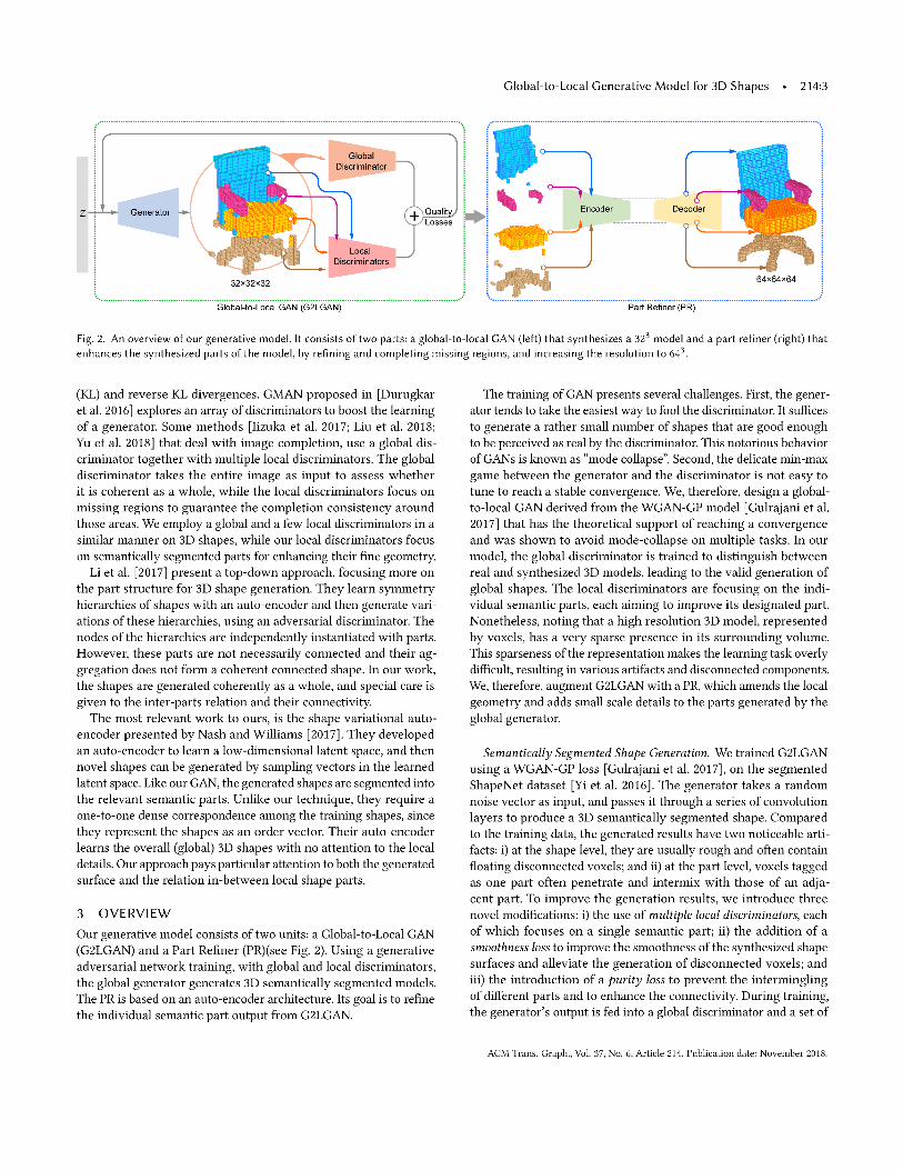
We introduce a generative model for 3D man-made shapes. The presented

method takes a global-to-local (G2L) approach. An adversarial network

(GAN) is built irst to construct the overall structure of the shape, segmented

and labeled into parts. A novel conditional auto-encoder (AE) is then aug-

mented to act as a part-level reiner. The GAN, associated with additional

local discriminators and quality losses, synthesizes a voxel-based model, and

assigns the voxels with part labels that are represented in separate channels.

The AE is trained to amend the initial synthesis of the parts, yielding more

plausible part geometries. We also introduce new means to measure and

evaluate the performance of an adversarial generative model. We demon-

strate that our global-to-local generative model produces signiicantly better

results than a plain three-dimensional GAN, in terms of both their shape

variety and the distribution with respect to the training data.

∗Joint irst authors2Corresponding author: Hui Huang (hhzhiyan@gmail.com)

Authors’ addresses: Hao Wang, Shenzhen University; Nadav Schor, Tel Aviv Univer-sity; Ruizhen Hu, Shenzhen University; Haibin Huang, Megvii / Face++ Research;Daniel Cohen-Or, Shenzhen University and Tel Aviv University; Hui Huang, College ofComputer Science & Software Engineering, Shenzhen University.

Permission to make digital or hard copies of all or part of this work for personal orclassroom use is granted without fee provided that copies are not made or distributedfor proit or commercial advantage and that copies bear this notice and the full citationon the irst page. Copyrights for components of this work owned by others than ACMmust be honored. Abstracting with credit is permitted. To copy otherwise, or republish,to post on servers or to redistribute to lists, requires prior speciic permission and/or afee. Request permissions from permissions@acm.org.

© 2018 Association for Computing Machinery.0730-0301/2018/11-ART214 $15.00https://doi.org/10.1145/3272127.3275025

CCS Concepts: · Computing methodologies→ Shape modeling;

Additional Key Words and Phrases: Shape modeling, generative adversarial

networks, semantic segmentation, global-to-local, part reiner

ACM Reference Format:

Hao Wang, Nadav Schor, Ruizhen Hu, Haibin Huang, Daniel Cohen-Or,

and Hui Huang. 2018. Global-to-Local Generative Model for 3D Shapes.

ACM Trans. Graph. 37, 6, Article 214 (November 2018), 10 pages. https:

//doi.org/10.1145/3272127.3275025

1 INTRODUCTION

Three-dimensional content creation has been a central research area

in computer graphics for decades. The main challenge is to minimize

manual intervention, while still allowing the creation of a variety of

plausible 3D objects. It is particularly challenging to create a novel

shape that appears to be sampled from the distribution of a given

class. It is hard to encapsulate the essence of a class of objects and

express it in a compact model to guide the creation of a sample in

the class. Common 3D generative techniques are based on existing

parts taken from objects in the class, and synthesizing novel shapes

by combining them, following probabilistic models or geometric

constraints [Chaudhuri et al. 2011; Kalogerakis et al. 2012].

The emergence of generative neural networks and, in particular,

adversarial networks [Goodfellow et al. 2014] ofers new means

to generate elements from a particular learned class. The key idea

is that instead of explicitly modeling the class, a discriminator is

trained to tell whether a generated model belongs to the target class

ACM Trans. Graph., Vol. 37, No. 6, Article 214. Publication date: November 2018.

214:2 • H. Wang, N. Schor, R. Hu, H. Huang, D. Cohen-Or and H. Huang

or not. The trained discriminator implicitly supervises the generator

to model the class distribution.

These generative adversarial networks (GANs) have recently

gained popularity in various domains and applications, showing

promising results. Generally speaking, GANs achieve reasonable

success in generating samples from a class distribution [Salimans

et al. 2016a]. Nonetheless, they typically lack the ability to synthe-

size the details well [Berthelot et al. 2017; Gulrajani et al. 2017]. The

problem is even more pronounced for GANs that aim at generat-

ing complex 3D man-made models [Liu et al. 2017; Wu et al. 2016].

Previous eforts in developing a 3D GAN for man-made objects

have partial success in modeling their 3D structures. However, they

behave rather poorly in modeling their iner geometric details, ex-

hibiting signiicant noise, outliers and disconnected or missing parts.

While the use of Hashing or Octree [Shao et al. 2018; Tatarchenko

et al. 2017] can improve the output resolution, we opted to use a sim-

ple and plain voxel representation, with a high enough resolution

to demonstrate the conceptual advancement of our approach.

In this work, we present a global-to-local generative model to

synthesize 3D man-made shapes; see Fig. 1 as an example. It is

based on an adversarial network to construct a global structure of

the shape, with local part labels. The global discriminator is trained

to distinguish between the whole real and generated 3D shapes,

while the local discriminators focus on the individual local parts.

A novel conditional auto-encoder is then introduced to enhance

the part synthesis. Speciically, The GAN synthesizes a voxel-based

model, and assigns part labels to each voxel. The auto-encoder acts

as a part-level reiner to amend the initial synthesis of each part.

To further enhance the shape generation, we introduce two more

new losses in addition to the adversarial loss. One encourages the

part compactness by measuring the purity of part regions, and the

other helps to improve the smoothness of the synthesized surface.

Nevertheless, the quality of the generated shapes is still rather low.

The resolution of the 3D shape generation is in general too low

to model ine details, like for example the blades of turbines of

an airplane or the hands and ingers of a human body. Our G2L

approach, however, introduces a conceptual advancement in the

generative modeling of man-made shapes.

The evaluation of our generative model, like any other GAN, is far

from trivial. The performance of a GAN should be measured by the

quality of each of the synthesized objects and by their overall variety

and agreement to the training data distribution. These measures

were overlooked in previous works. We introduce new means to

measure and evaluate the performance of an adversarial generative

model, and demonstrate that our system produces signiicantly

better results than a plain three-dimensional GAN.

2 RELATED WORK

2.1 Assembly-based Shape Synthesis

There are numerous works that create new 3Dmodels by assembling

from existing components. The pioneer work [Funkhouser et al.

2004] composes shapes by retrieving relevant shapes from a reposi-

tory, then cuts and extracts components from these shapes and glues

them together to form a new shape. The following works [Chaud-

huri and Koltun 2010; Fish et al. 2014; Huang et al. 2015; Kalogerakis

et al. 2012; Kim et al. 2013; Talton et al. 2012; Xu et al. 2012] try to

improve the modeling process with more sophisticated techniques

that consider the part relations or shape structures, e.g., employing

Bayesian networks or modular templates. We refer to a STAR re-

port [Mitra et al. 2013] for an overview of works on this aspect. The

technique we propose here is also data-driven, but it trains a GAN

to synthesize 3D shapes, rather than assembling existing parts.

2.2 Generative Neural Networks

With the development of deep learning techniques, there has been

a surge of research interest in deep generative models in recent

years. Deep generative models based on variational auto-encoders

(VAE) [Kingma and Welling 2014] or generative adversarial net-

works (GAN) [Goodfellow et al. 2014] havemade remarkable progress

in image generation problems [Isola et al. 2017; Radford et al. 2015;

Wang and Gupta 2016; Yan et al. 2016; Zhu et al. 2016]. With the

recent introduction of large publicly available 3D model reposito-

ries [Chang et al. 2015; Wu et al. 2015], there have been attempts to

generate 3D shapes using similar methods.

Most existing methods explore the problem of 3D reconstruction

from a given 2D image or sketch. Girdhar et al. [2016] combine a

3D auto-encoder with an image encoder, to map 3D shapes and 2D

images together into a common latent space to build the connection,

so that 3D shapes can be encoded given new 2D images. Wu et

al. [2017] propose a disentangled, two-step end-to-end trainable

model that sequentially estimates 2.5D sketches and a 3D object

shape from a given image. Instead of working on a volumetric rep-

resentation of 3D shapes, Fan et al. [2017] propose using a point

cloud representation for the reconstructed 3D shapes from a single

image to encode more geometric details, without adding much com-

putational overhead. Lin et al. [2018] further increase the eiciency

by introducing a diferentiable pseudo-renderer for 3D generation.

2.3 Learning-based Shape Synthesis

More related to our method are adversarial networks that learn to

generate 3D shapes from noise input directly [Li et al. 2017; Nash

and Williams 2017; Wu et al. 2016]. Wu et al. [2016] are the irst

to extend GAN for 3D shape generation, which shows that the

generator can capture the object structure implicitly and synthesize

plausible 3D objects. Nonetheless, without explicitly constraining

the part structures, semantic validation of the generated shapes

cannot be guaranteed and important structure properties cannot be

well-preserved during the generation.

CommonGANnetworks consist of one generator and one discrim-

inator. Recently, Some recent attempts have been made to combine

multiple discriminators or generators together. Hoang et al. [2017]

train multiple generators to explore diferent modes of the data

distribution. The array of generators shares their parameters and a

softmax classiier is used to classify which generator the data comes

from. Similarly, MIX+GAN proposed in [Arora et al. 2017] uses a

mixture of generators to enforce the generated distribution to be of

higher diversity. In contrast, the combination of multiple discrimina-

tors and a single generator aims at constructing a stronger discrim-

inator to guide the generator. D2GAN proposed in [Nguyen et al.

2017] employs two discriminators to optimize both Kullback-Leibler

ACM Trans. Graph., Vol. 37, No. 6, Article 214. Publication date: November 2018.

214:4 • H. Wang, N. Schor, R. Hu, H. Huang, D. Cohen-Or and H. Huang

local discriminators. The global discriminator evaluates the quality

of the overall shape, while each local discriminator focuses on its

dedicated semantic part. All the global and local discriminators are

trained simultaneously.

Part-wise Reinement. The G2LGAN generates semantically seg-

mented models. We then separate the diferent semantic parts, and

feed them part-by-part to the part reiner. The PR is trained to en-

code a given, possibly rough or incomplete part, into a latent vector

and decode it back into a complete part. To train a universal PR

for all diferent types of parts, we concatenate the part label to the

latent vector that encodes the part. The PR reines two aspects of

the generated parts; i) the resolution of the input part is enlarged

from 323 to 643 to generate iner details in the model; and ii) rough

or incomplete parts become smoother and are illed as needed.

4 METHOD

4.1 Generator and Discriminators

We adopt the WGAN-GP [Gulrajani et al. 2017] as the base architec-

ture of the generator. The generator takes a random noise vector

z ∈ R200 as input. It consists of four transposed convolution lay-

ers. We use ilter size of 43 with strides [1, 1, 1] for the irst layer

and [2, 2, 2] for the other layers. We use batch normalization and

a ReLU activation function after each of the irst three transposed

convolution layers. We use softmax as the activation function of

the last layer. The generator outputs a volume of 323 × C , where

C denotes the number of semantic parts in the segmented model.

Each voxel is represented by a probability vector, with the length of

C . Each channel corresponds to a part label. When we visualize the

generated models, we assign each voxel with the part label that has

the highest probability.

The two main well-known artifacts caused by a vanilla generator,

are rough models and voxels intermingling between the diferent

model parts. To improve the performance, we introduce global-to-

local discriminators and two new quality loss terms to help guide

the generator to produce decent results.

The global discriminator has four convolution layers, with a ilter

size of 43. The irst three layers use strides of [2, 2, 2] and a leaky

ReLU, while the last layer uses strides of [1, 1, 1] and no activation

layer. We use a batch size of 64, and Adam optimizer with settings

recommended in [Gulrajani et al. 2017], i.e., learning rate = 1e−4,

β1 = 0.5, β2 = 0.9, λ = 10 and ive discriminator iterations.

The local discriminators follow the same pattern of the global

discriminator, except that their inputs are semantically segmented

parts instead of a whole shape. The softmax output of the gener-

ator G (z) is converted into multiple-channel one-hot vector. The

multiple-channel vector is then split into single channel vectors,

serving as binary attention masks {Mi } for diferent parts. By the

element-wise multiplication between the attention mask and soft-

max output, i.e., G (z) ◦Mi , local discriminators only focus on their

corresponding semantic parts.

By assigning diferent weights for the global and local discrimi-

nators, their combinations are trained jointly to guide the generator

synthesizing shapes with enhanced global structure and more ine

0 1 0 2 1 1 1

1 4 3 3 0 1 1

0 3 3 4 1 1 1

1 2 0 1 0 1 1

1 1 1 1 1 1 1

1 2 2 1 2 1 1

1 2 1 0 1 2 1

0 1 0 2 1 1 1

1 4 3 3 4 1 1

0 3 4 4 1 1 1

1 2 1 1 2 2 1

1 2 1 2 4 3 1

1 3 2 1 2 2 1

1 2 1 0 1 2 1

- - - - 0 0 -

- 0 - 0 4 0 -

- - 1 - 0 0 -

- 0 1 0 2 1 -

- 1 0 1 3 2 -

- 1 - - - 1 -

- 0 - - - 0 -

(a) smoothness (b) purity (c) combination

Fig. 3. Voxels contribution to the diferent losses: (a) smoothness, (b) pu-

rity, and (c) their combination. The value inside each voxel represents its

contribution to the specific loss. As can be seen from (a) and (b), the voxels

that have the highest values (shown in bold) are the most problematic ones,

floating or intermingling. The summary of the voxels contribution is shown

in (c), where a voxel is marked in bold, if it was marked in bold in (a) or (b).

scale details. Our adversarial loss function is thus deined as:

La = Lglobal +

c∑

i=1

wiLilocal, (1)

whereLglobal andLilocal

are set as the same in [Gulrajani et al. 2017].

In all our experiments, we setwi = 1 for all the categories.

4.2 uality Losses

The main goal of adding the quality losses, i.e., smoothness and

purity losses, is to penalize the generator based on the efect of each

individual voxel in the generated model. We would like to compute

the contribution of each voxel on the artifacts of the vanilla GAN.

As can be seen from Fig. 3, the unwanted voxels receive the highest

values, and thus have a larger efect on the losses.

Note that since the generated shapes are eventually visualized

by assigning each voxel with the label of maximal probability and

using the softmax output as a means to compute the penalty of each

voxel may lead to closer label distributions between neighboring

voxels, while still maintaining their original unwanted label, we

decided to penalize the intractable voxels, using the equivalent one-

hot representation, instead of the direct softmax results. However,

since converting a softmax output into a one-hot vector is not a

diferentiable operation, we use a sigmoid function, centered at

0.5, with a steep slope to approximate the one-hot representation:

sig(x ) = 1/(1 + e−100(x−0.5) ).

Smoothness Loss. We introduce the smoothness loss to smooth

the generated models and reduce the number of loating voxels. In

this loss, we ignore the part labels and treat the model as one (un-

segmented) global shape. We consider the relation and connectivity

between the object and its background, and deine the Smoothness

Contribution (Sc ) of each voxel, as the sum of L1 distances between

its approximate one-hot label vector and those of its adjacent voxels;

see Fig. 3(a). Meanwhile, we set a threshold ηs (= 2.89 by default)

to avoid penalizing border voxels, i.e., ∀x , Sc (x ) = 0, if Sc (x ) < ηs .

The smoothness loss follows as:

Ls =∑

x

(Sc (x ))2, (2)

ACM Trans. Graph., Vol. 37, No. 6, Article 214. Publication date: November 2018.

Global-to-Local Generative Model for 3D Shapes • 214:5

where we square Sc (x ) to achieve an exponential diference between

loating voxels and voxels that stick out of the model’s surface.

Purity Loss.We introduce the purity loss to prevent intermingling

between diferent parts. In this loss, we ignore the background

voxels and consider only the object voxels. We deine the Purity

Contribution (Pc ) of each voxel, as the sum of L1 distances between

its approximate one-hot label vector and those of its adjacent parts

voxels; see Fig. 3(b). Again, we deine a threshold ηp (= 1.69 by

default) to avoid penalizing border voxels, i.e., ∀x , Pc (x ) = 0, if

Pc (x ) < ηp . The purity loss follows as:

Lp =∑

x

(Pc (x ))2, (3)

where, similar to (2), we square Pc (x ) to achieve an exponential

diference between the diferent levels of voxels intermingling.

Our Generator Loss is thus deined as a weighted sum of the

aforementioned three losses (1), (2), and (3):

Lдen = La +wsLs +wpLp , (4)

where we setws = 0.05 andwp = 0.0667 by default.

4.3 Part Refiner

We use an auto-encoder architecture with a reconstruction loss as a

Part Reiner (PR). The PR receives a part with its label to produce

a reined model of that part. The input part is represented as a 323

volume, the label is a one-hot vector and the output part is a volume

of size 643. We use three convolution layers, with ilter size 43 and

strides of [2, 2, 2], followed by a FC layer, to encode the input part

into a 128-dimension latent space. We use three 128-dimensional

FC layers to encode the part-label vector. The two 128-vectors are

then concatenated and fed through two 256-dimensional FC layers

to combine the encoding of both inputs. The decoder consists of

ive transposed convolution layers with a ilter size of 43 and strides

of [2, 2, 2]. We use batch normalization and ReLU, after each layer

in both the encoder and decoder.

To compute the reconstruction loss, we need to have both the

input, i.e., part and label, and the expected output. We can generate

trivial pairs from the training set, where the input is from the 323

resolution samples and the output is taken from the same model, but

at 643 resolution. To grant the PR ability to reine imperfect parts,

we further construct a second training set by pairing imperfect parts

and their perfect counterparts. We randomly generate 1,024 models

using the trained G2LGAN and separate them into diferent parts

as inputs to the PR. As the expected outputs, for each generated

part, we retrieve its 3-nearest-neighbors (to prevent the PR from

memorizing a one-to-one mapping) from the 323 training set, and

then use their corresponding 643 representations. At training time,

when a generated part is fed into the PR, an average voxel-wise

cross-entropy is computed as the reconstruction loss by comparing

the output to one of the input’s nearest-neighbors, picked randomly.

When searching for those pairing nearest neighbors, we would

also like to enable our PR to map a given part into an empty output,

so that it can remove noise or small unorganized part outliers. To

achieve this, we separate the generated parts into three categories:

empty parts, parts that consist of only few (less than 10 by default)

voxels, and the remaining parts. We directly remove the empty parts

from the training set, since we do not want to burden our model

with learning empty-to-empty mapping. The parts that consist of a

few voxels would be very likely a noise or outlier, for which we aim

to clean up by mapping them to an empty part. Thus, as a metric to

ind the nearest-neighbors, we use L1 distance for these suspicious

parts, allowing a mapping to an empty volume. For the remaining

parts, we use the Intersection-over-Union (IoU) metric instead. The

random noise may accidentally intersect with diferent parts in the

training set and be paired to them instead of an empty part since the

IoU with an empty part is always zero. We use the Adam optimizer

for training, with a batch size of 64 and a learning rate of 5e−5.

5 RESULTS AND EVALUATION

To evaluate our method, we set up two baselines. The irst is [Wu

et al. 2015] with one modiication, referred to as 3DGAN, which

outputs C channels for every voxel instead of one. We train the

3DGAN as presented in the paper. The second one, referred to as

Baseline, is similar to G2LGAN without the local discriminators and

the quality losses. The Baseline’s discriminator is identical to the

global discriminator of G2LGAN (see Sec. 4.1). We use a batch size of

64, and an Adam optimizer with settings recommended in [Gulrajani

et al. 2017], i.e., learning rate = 1e−4, β1 = 0.5, β2 = 0.9, λ = 10 and

5 discriminator iterations. We present randomly picked generated

results from both two baselines in the supplementary material.

5.1 Training Sets and Generation Results

We build our training set from a collection of 3D meshes on four

categories: Chair (900), Airplane(2690), Lamp(1546), and Table(5256).

These models are taken from ShapeNet [Chang et al. 2015], which

have been consistently aligned, scaled, and semantically segmented.

The semantic labels are from [Huang et al. 2015], and each object

category has a ixed number of semantic parts: four parts (back,

seat, leg, armrest) for Chair; four parts (body, wing, tail, engine) for

Airplane; four parts (base, shade, canopy and tubing) for Lamp; and

three parts (top, leg and drawer) for Table. Individual shapes may or

may not contain all of these parts. By combining these 3D meshes

and their part label information together, we voxelize them to form

our volumetric training sets with corresponding semantic indexes.

After training, we generate 1024(= 64 × 16) new models for

each object category. Recall that the goal of the generator in a

GAN setting is to learn the mapping from a latent space to the

distribution of the training data. Thus, to show some representative

results, we deine a conidence score for each generated shape. More

speciically, for each category, we irst train a shape-level auto-

encoder to extract a feature representation for each of the training

shapes, and perform K-Means on the whole training set to get 10

clusters. We train a classiier to map each of the training shapes

into one of the clusters. For each generated shape, we then deine

the highest Softmax probability obtained from the classiier, as its

conidence score.

ACM Trans. Graph., Vol. 37, No. 6, Article 214. Publication date: November 2018.

214:6 • H. Wang, N. Schor, R. Hu, H. Huang, D. Cohen-Or and H. Huang

Fig. 4. A gallery of our generated Chairs, Airplanes, Lamps, and Tables shown above, with their 3-nearest-neighbors retrieved from the training set.

Fig. 5. PR Improvement. For each category, we present four examples of the improvement achieved by the PR. Shapes generated by G2LGAN are shown on

the top row, and their PR enhanced versions are provided underneath for a clear comparison.

In Fig. 4, for each category, we present a set of representative

generated shapes located in diferent clusters, which have the high-

est conidence scores in the top row and retrieve the 3-nearest-

neighbors from the training set for each shape to show below for

a visual quality comparison. The shape matching distance is com-

puted as the average of the Chamfer distances [Fan et al. 2017] over

all paired semantic parts. As we can see, our generated shapes look

similar to their closest training neighbors, i.e., with high validity,

yet also contain meaningful variations in geometry. More generated

results are shown in the supplementary material.

It is worth emphasizing that our PR cannot only increase the

output resolution to 643, but also add important missing ine details

while cleaning up noisy components; see Fig. 5, where we can clearly

observe the signiicant reduction of noise and reined details. More

examples are included in the supplementary material.

5.2 uantitative Evaluation on Shape Synthesis

We present three diferent evaluation metrics to quantitatively eval-

uate the variety and quality of our synthesized shapes. The irst

metric (3D inception score) evaluates the variety and quality of the

ACM Trans. Graph., Vol. 37, No. 6, Article 214. Publication date: November 2018.

Global-to-Local Generative Model for 3D Shapes • 214:7

Table 1. Inception and Symmetry comparisons of generated chairs. Both

baselines receive lower scores in all categories, in comparison to our models,

G2LGAN and G2LGAN+PR. Local Discriminators (LD) beter improve the

Baseline in the symmetry score for Leg and Arm while theuality Losses

(QL) beter improve the other categories.

Models InceptionSymmetry

Shape Back Seat Leg Arm

3DGAN 5.84 0.70 0.71 0.76 0.35 0.16

Baseline (BL) 5.55 0.78 0.76 0.80 0.55 0.51

BL & LD 5.62 0.80 0.78 0.80 0.64 0.63

BL & QL 5.99 0.82 0.82 0.85 0.60 0.53

G2LGAN 6.00 0.84 0.83 0.85 0.63 0.66

G2LGAN+PR 6.17 0.91 0.93 0.94 0.71 0.64

GT 8.16 0.96 0.93 0.94 0.84 0.84

generated shape set, the second metric (symmetry score) evaluates

the symmetry of the synthesized parts, and the third metric (dis-

tribution distance) uses a few statistical measures to evaluate the

distance between the synthesized shapes and the training set.

3D Inception Score. The inception scorewas irst introduced by [Sal-

imans et al. 2016b] and is commonly used for evaluating gener-

ated images. The score is based on the inception classiication net-

work [Szegedy et al. 2016] which was pre-trained on the ImageNet

dataset. It measures both the variety of the generated content and

its quality, based on the conidence of the classiier and the variance

of the generated classes.

Since the generated 3D models are from a single category and the

inception score is deined based on a classiier, we cannot directly

apply the computation of the inception score to our data. However,

as described in Section 5.1, we can cluster the training data from

the same category into 10 clusters, and then consider the clusters as

diferent classes to train the corresponding 3D inception classiica-

tion network for computing the inception score. For the PR output,

which is in higher resolution 643, we down-sample it to 323 irst and

then compute the inception score. As we can see from Table 1, the

PR improves the inception score of the G2LGAN model and receives

a higher score than the baseline models. Although the 3DGAN base-

line obtains a better inception score than the Baseline and Baseline

with local discriminators, its results for the symmetry are the lowest

and its visual results, e.g., shown in the supplementary material, are

extremely poor in comparison to our models.

Symmetry Score. All the categories that were tested are man-made

objects, thus, they are more likely to have a symmetric structure,

as we can see from the symmetry score of the training data (GT) in

the bottom row of Table 1. It is, therefore, expected that generated

model should also demonstrate the appropriate symmetry.

We only evaluate bilateral symmetry here and deine the sym-

metry score as the percentage of voxels which got matched after a

relectance transformation given a symmetry plane. Since all the

shapes in each category are aligned, we set a ixed symmetry plane

for all of the training and generated shapes for the same category.

We then compute the corresponding symmetry score for each se-

mantic part and the global shape. We can see in Table 1 that the

5 151� 2� 25 3� 35 4� 5 151� 2� 25 3� 35 4� 5 151� 2� 25 3� 35 4�

5 151� 2� 25 3� 35 4�

1�-�

1�-�

1�-�

1�-�

1�-�

1�-�

1�-�

1�-�

1�-�

1�-�

1�-�

1�-�

B������ G2G��3 G��

A����������� A�����������A�����������

5 151� 2� 25 3� 35 4�1�-�

1�-�

1�-�

������������������

5 151� 2� 25 3� 35 4�1�

1�

1�

-�

-�

-�

���������

Fig. 6. Comparison on the JSD of pair-wise features of the generated shapes

from the baselines and G2LGAN relative to the training data. The horizontal

axis represents the number of clusters and the vertical axis represents the

JSD value. Smaller values are beter.

Back Seat Legs

0

0.1

0.2

0.3

0.5

0.4

5 1510 20 25 30 35 400

0.1

0.2

0.3

0.5

0.4

5 1510 20 25 30 35 400

0.1

0.2

0.3

0.5

0.4

5 1510 20 25 30 35 400

0.1

0.2

0.3

0.5

0.4

5 1510 20 25 30 35 40

Armrest

Baseline G2LGAN3DGAN

Fig. 7. Comparison on the JSD of part-wise features of the generated shapes

from the baselines and G2LGAN relative to the training data. The horizontal

axis represents the number of clusters and the vertical axis represents the

JSD value. Smaller values are beter.

JS

D

0

0.1

0.2

0.3

0.4

0.5

0.6

0.7

5 1510 20 25 30 35 40

Baseline

G2LGAN

G2LGAN +PR

3DGAN

Fig. 8. Comparison on the JSD of component-wise features of the gener-

ated shapes from the baselines, G2LGAN and G2LGAN+PR relative to the

training data. The horizontal axis represents the number of clusters and the

vertical axis represent the JSD value. Smaller values are beter.

symmetry scores of our method are consistently higher than those

of the baseline models.

ACM Trans. Graph., Vol. 37, No. 6, Article 214. Publication date: November 2018.

214:10 • H. Wang, N. Schor, R. Hu, H. Huang, D. Cohen-Or and H. Huang

Ishan Durugkar, Ian Gemp, and Sridhar Mahadevan. 2016. Generative multi-adversarialnetworks. arXiv preprint arXiv:1611.01673 (2016).

Haoqiang Fan, Hao Su, and Leonidas J Guibas. 2017. A Point Set Generation Networkfor 3D Object Reconstruction From a Single Image. In Proc. IEEE Conf. on ComputerVision & Pattern Recognition. 605ś613.

Noa Fish, Melinos Averkiou, Oliver van Kaick, Olga Sorkine-Hornung, Daniel Cohen-Or,and Niloy J. Mitra. 2014. Meta-representation of Shape Families. ACM Trans. onGraphics 33, 4 (2014), 34:1ś34:11.

Thomas Funkhouser, Michael Kazhdan, Philip Shilane, Patrick Min, William Kiefer,Ayellet Tal, Szymon Rusinkiewicz, and David Dobkin. 2004. Modeling by Example.ACM Trans. on Graphics 23, 3 (2004), 652ś663.

Rohit Girdhar, David F Fouhey, Mikel Rodriguez, and Abhinav Gupta. 2016. Learning apredictable and generative vector representation for objects. In Proc. Euro. Conf. onComputer Vision. 484ś499.

Ian J. Goodfellow, Jean Pouget-Abadie, Mehdi Mirza, Bing Xu, David Warde-Farley,Sherjil Ozair, Aaron Courville, and Yoshua Bengio. 2014. Generative AdversarialNets. In Advances in Neural Information Processing Systems (NIPS). 2672ś2680.

Ishaan Gulrajani, Faruk Ahmed, Martin Arjovsky, Vincent Dumoulin, and Aaron CCourville. 2017. Improved training of wasserstein gans. In Advances in NeuralInformation Processing Systems (NIPS). 5769ś5779.

Quan Hoang, Tu Dinh Nguyen, Trung Le, and Dinh Phung. 2017. Multi-GeneratorGernerative Adversarial Nets. arXiv preprint arXiv:1708.02556 (2017).

Haibin Huang, Evangelos Kalogerakis, and Benjamin Marlin. 2015. Analysis andSynthesis of 3D Shape Families via Deep-learned Generative Models of Surfaces.Computer Graphics Forum 34, 5 (2015), 25ś38.

Satoshi Iizuka, Edgar Simo-Serra, and Hiroshi Ishikawa. 2017. Globally and LocallyConsistent Image Completion. ACM Trans. on Graphics 36, 4 (2017), 107:1ś107:14.

Phillip Isola, Jun-Yan Zhu, Tinghui Zhou, and Alexei A. Efros. 2017. Image-to-ImageTranslation with Conditional Adversarial Networks. Proc. IEEE Conf. on ComputerVision & Pattern Recognition (2017), 5967ś5976.

Evangelos Kalogerakis, Siddhartha Chaudhuri, Daphne Koller, and Vladlen Koltun.2012. A Probabilistic Model for Component-based Shape Synthesis. ACM Trans. onGraphics 31, 4 (2012), 55:1ś55:11.

Vladimir G. Kim, Wilmot Li, Niloy J. Mitra, Siddhartha Chaudhuri, Stephen DiVerdi, andThomas Funkhouser. 2013. Learning Part-based Templates from Large Collectionsof 3D Shapes. ACM Trans. on Graphics 32, 4 (2013), 70:1ś70:12.

Diederik P Kingma and Max Welling. 2014. Auto-Encoding Variational Bayes. In Proc.Int. Conf. on Learning Representations.

Jun Li, Kai Xu, Siddhartha Chaudhuri, Ersin Yumer, Hao Zhang, and Leonidas Guibas.2017. GRASS: Generative Recursive Autoencoders for Shape Structures. ACM Trans.on Graphics 36, 4 (2017), 52:1ś52:14.

Chen-Hsuan Lin, Chen Kong, and Simon Lucey. 2018. Learning Eicient Point CloudGeneration for Dense 3D Object Reconstruction. In AAAI Conference on ArtiicialIntelligence (AAAI).

Guilin Liu, Fitsum A Reda, Kevin J Shih, Ting-Chun Wang, Andrew Tao, and BryanCatanzaro. 2018. Image Inpainting for Irregular Holes Using Partial Convolutions.arXiv preprint arXiv:1804.07723 (2018).

Jerry Liu, Fisher Yu, and Thomas Funkhouser. 2017. Interactive 3D modeling with agenerative adversarial network. In Proc. Int. Conf. on 3D Vision. 126ś134.

Niloy Mitra, Michael Wand, Hao (Richard) Zhang, Daniel Cohen-Or, Vladimir Kim, andQi-Xing Huang. 2013. Structure-aware Shape Processing. In SIGGRAPH Asia 2013Courses. 1:1ś1:20.

C. Nash and C. K. I. Williams. 2017. The Shape Variational Autoencoder: A DeepGenerative Model of Part-segmented 3D Objects. Computer Graphics Forum 36, 5(2017), 1ś12.

Tu Nguyen, Trung Le, Hung Vu, and Dinh Phung. 2017. Dual discriminator generativeadversarial nets. In Advances in Neural Information Processing Systems (NIPS). 2667ś2677.

Charles R Qi, Hao Su, KaichunMo, and Leonidas J Guibas. 2017. Pointnet: Deep learningon point sets for 3D classiication and segmentation. Proc. IEEE Conf. on ComputerVision & Pattern Recognition (2017), 652ś660.

Alec Radford, Luke Metz, and Soumith Chintala. 2015. Unsupervised representationlearning with deep convolutional generative adversarial networks. arXiv preprintarXiv:1511.06434 (2015).

Tim Salimans, Ian Goodfellow, Wojciech Zaremba, Vicki Cheung, Alec Radford, andXi Chen. 2016a. Improved Techniques for Training (GANs). In Advances in NeuralInformation Processing Systems (NIPS). 2234ś2242.

Tim Salimans, Ian Goodfellow, Wojciech Zaremba, Vicki Cheung, Alec Radford, andXi Chen. 2016b. Improved Techniques for Training (GANs). In Advances in NeuralInformation Processing Systems (NIPS). 2234ś2242.

Tianjia Shao, Yin Yang, YanlinWeng, Qiming Hou, and Kun Zhou. 2018. H-CNN: SpatialHashing Based CNN for 3D Shape Analysis. arXiv preprint arXiv:1803.11385 (2018).

Robert W. Sumner, Johannes Schmid, and Mark Pauly. 2007. Embedded Deformationfor Shape Manipulation. ACM Trans. on Graphics 26, 3 (2007), 80:1ś80:7.

Christian Szegedy, Vincent Vanhoucke, Sergey Iofe, Jon Shlens, and Zbigniew Wojna.2016. Rethinking the inception architecture for computer vision. In Proc. IEEE Conf.

on Computer Vision & Pattern Recognition. 2818ś2826.Jerry Talton, Lingfeng Yang, Ranjitha Kumar, Maxine Lim, Noah Goodman, and Radomír

Měch. 2012. Learning Design Patterns with Bayesian Grammar Induction. In Proc.ACM Symp. on User Interface Software and Technology. 63ś74.

Maxim Tatarchenko, Alexey Dosovitskiy, and Thomas Brox. 2017. Octree generatingnetworks: Eicient convolutional architectures for high-resolution 3D outputs. InProc. Int. Conf. on Computer Vision. 2088ś2096.

Xiaolong Wang and Abhinav Gupta. 2016. Generative image modeling using style andstructure adversarial networks. In Proc. Euro. Conf. on Computer Vision. 318ś335.

JiajunWu, YifanWang, Tianfan Xue, Xingyuan Sun, Bill Freeman, and Josh Tenenbaum.2017. Marrnet: 3D shape reconstruction via 2.5D sketches. In Advances in NeuralInformation Processing Systems (NIPS). 540ś550.

Jiajun Wu, Chengkai Zhang, Tianfan Xue, William T. Freeman, and Joshua B. Tenen-baum. 2016. Learning a Probabilistic Latent Space of Object Shapes via 3DGenerative-adversarial Modeling. In Advances in Neural Information ProcessingSystems (NIPS). 82ś90.

Zhirong Wu, Shuran Song, Aditya Khosla, Fisher Yu, Linguang Zhang, Xiaoou Tang,and Jianxiong Xiao. 2015. 3d shapenets: A deep representation for volumetric shapes.In Proc. IEEE Conf. on Computer Vision & Pattern Recognition. 1912ś1920.

Kai Xu, Hao Zhang, Daniel Cohen-Or, and Baoquan Chen. 2012. Fit and Diverse: SetEvolution for Inspiring 3D Shape Galleries. ACM Trans. on Graphics 31, 4 (2012),57:1ś57:10.

Xinchen Yan, Jimei Yang, Kihyuk Sohn, and Honglak Lee. 2016. Attribute2image:Conditional image generation from visual attributes. In Proc. Euro. Conf. on ComputerVision. 776ś791.

Li Yi, Vladimir G. Kim, Duygu Ceylan, I-Chao Shen, Mengyan Yan, Hao Su, CewuLu, Qixing Huang, Alla Shefer, and Leonidas Guibas. 2016. A Scalable ActiveFramework for Region Annotation in 3D Shape Collections. ACM Trans. on Graphics35, 6 (2016), 210:1ś210:12.

Jiahui Yu, Zhe Lin, Jimei Yang, Xiaohui Shen, Xin Lu, and Thomas S. Huang. 2018.Generative Image Inpainting With Contextual Attention. In Proc. IEEE Conf. onComputer Vision & Pattern Recognition. 5505ś5514.

Jun-Yan Zhu, Philipp Krähenbühl, Eli Shechtman, and Alexei A Efros. 2016. Generativevisual manipulation on the natural image manifold. In Proc. Euro. Conf. on ComputerVision. 597ś613.

ACM Trans. Graph., Vol. 37, No. 6, Article 214. Publication date: November 2018.