Global warming and hyperbolic discountingkarp/JpubEcon05.pdfmoderate discount rates, large future...

www.elsevier.com/locate/econbase

Journal of Public Economics 89 (2005) 261–282

Global warming and hyperbolic discounting

Larry Karp

207 Giannini Hall, University of California, Berkeley, CA 94720, USA

Received 17 December 2002; received in revised form 20 January 2004; accepted 10 February 2004

Available online 18 August 2004

Abstract

The use of a constant discount rate to study long-lived environmental problems such as global

warming has two disadvantages: the prescribed policy is sensitive to the discount rate, and with

moderate discount rates, large future damages have almost no effect on current decisions. Time-

consistent quasi-hyperbolic discounting alleviates both of these modeling problems, and is a

plausible description of how people think about the future. We analyze the time-consistent Markov

Perfect equilibrium in a general model with a stock pollutant. The solution to the linear-quadratic

specialization illustrates the role of hyperbolic discounting in a model of global warming.

D 2004 Elsevier B.V. All rights reserved.

JEL classification: D83; L50

Keywords: Stock pollutant; Hyperbolic discounting; Global warming; Time consistency

1. Introduction

There are two important consequences of using a constant discount rate to model the

control of long-lived environmental stocks such as greenhouse gasses. First, the optimal

program is likely to be sensitive to the discount rate; a parameter about which there is

some disagreement. Second, discounting at a non-negligible rate makes the present value

of future damages small. The effects of greenhouse gasses might not be felt for a century

(if ever). At an annual discount rate of 1%, we would invest 37 cents today to avoid a

dollar’s worth of damages in a century, and at a discount rate of 4% that amount falls to 1.8

cents. These values differ by a factor of more than 20. The corresponding values if

damages occur after 10 years rather than after a century are 90 and 67 cents, numbers that

0047-2727/$ - see front matter D 2004 Elsevier B.V. All rights reserved.

doi:10.1016/j.jpubeco.2004.02.005

E-mail address: [email protected] (L. Karp).

L. Karp / Journal of Public Economics 89 (2005) 261–282262

differ by a factor of less than 1.4. The cost-benefit ratio for investments related to global

warming may be largely determined by the discount rate.

It seems reasonable to apply a non-negligible discount to the future, but using a constant

and non-negligible discount rate make us callous toward the far-distant future. An obvious

remedy is to use a declining discount rate. This remedy introduces the problem of time-

inconsistency. A time-consistent equilibrium can be studied, but even with strong

assumptions such as Markov beliefs and differentiable policies, this equilibrium is typically

not unique in an infinite horizon problem. Despite this limitation, discounting is sufficiently

important in problems of long-lived pollutants that it is worth considering carefully an

alternative to constant discounting. This paper is a step towards providing that analysis.

Section 2 reviews the literature, and explains why hyperbolic discounting is a useful

way to model long-lived environmental problems. Section 3 uses Harris and Laibson

(2001)’s heuristic method to derive the Euler equation in a stock-pollutant model. This

section provides sufficient conditions under which the expected stock either oscillates or

changes monotonically. The section then discusses the non-uniqueness and the Pareto

ranking of the set of differentiable Markov perfect equilibria (MPE). Section 4 specializes

the model to linear-quadratic functions and presents the equations that determine the

(linear) equilibrium decision rule. A calibration that represents plausible magnitudes of

costs and benefits associated with global warming shows that hyperbolic discounting

provides a useful method of studying long-lived environmental problems.

To the extent that a social planner has a declining discount rates, the analysis here is

positive. The paper may also contribute to the large normative literature on the optimal

control of greenhouse gasses, which assumes a constant discount rate. If a decreasing

discount rate provides a better description of society’s preferences, and if the time-

consistency problem is important, then the model studied here is useful for normative

analysis.

2. Literature review

Arrow et al. (1996) suggest that the appropriate discount rate for environmental

damages in the distant future depends on whether the modeling exercise is ‘‘descriptive’’

or ‘‘prescriptive’’. They conclude that in the former case, it is appropriate to use a market

rate of interest, typically in excess of 7%; in the latter case, a social discount rate no greater

than 3% should be used. The collection of papers edited by Portney and Weyant (1999)—

in particular, Dasgupta et al. (1999); Cline (1999)—provides a variety of perspectives on

this issue. Heal (1998, 2001) examines the effect of different kinds of discounting in

environmental contexts. Frederick et al. (2002) review the genesis of models based on

discounted utility, and they survey the empirical literature that measures individuals’

discount rates.

Cropper and Laibson (1999) suggest using hyperbolic discounting to evaluate payoffs

under global warming. They use Phelps and Pollack (1968)’s model in which an individual

chooses a time-profile of consumption, subject to a growth rate for capital. We use a

similar idea, but modify the model so that it describes a situation in which the

accumulation of a pollution stock causes future economic damages.

L. Karp / Journal of Public Economics 89 (2005) 261–282 263

In a continuous time setting, where U(ct) is the social utility of consumption and /(t) isthe discount factor for consumption, the payoff at time t is ml0 /ðsÞUðctþsÞds. The presentvalue today of $1 additional consumption s units of time in the future is / (s)UV(ct + s). The

social discount rate, r(t), equals the negative of the rate of change of the present value of

future marginal utility of consumption:

rðtÞ ¼ �dlnð/ðtÞUVðctÞÞdt

¼ nðtÞ þ tðctÞcðtÞcðtÞ ; ð1Þ

where n(t) is the pure rate of time preference and t(c) is the elasticity of marginal utility of

consumption. In standard usage, hyperbolic discounting refers to a falling pure rate of time

preference. This paper interprets hyperbolic discounting as a declining social discount rate.

Rabin (1998) describes the psychological basis for a declining pure rate of time

preference. Ainslie (1991); Cropper et al. (1994); Kirby and Herrenstein (1995) provide

empirical evidence that individuals actually discount the future in this manner. Read

(2001); Rubinstein (2003) offer other interpretations of this evidence. Rubinstein presents

experimental evidence that is not consistent with either constant or hyperbolic discounting,

but is consistent with a decision-making procedure based on ‘‘similarity relations’’. This

procedure assumes that individuals ignore small differences and focus on large differences

when comparing two alternatives.

Hyperbolic discounting and ‘‘similarity relations’’ models have important differences,

but they have in common the idea that a decision-maker’s ability to distinguish between

the levels of characteristics of alternatives is important in making a choice. Hyperbolic

discounting assumes that the ability to make distinctions diminishes for more distant

events. For example, an individual might prefer $1 today to $2 tomorrow; in a short time

frame, a single day is an appreciable delay. The same individual might prefer to receive $2

in 10 years and 1 day rather than $1 in 10 years; over a long time frame, the elapse of a

single day is nearly irrelevant.

This idea is compelling when considering long-lived environmental problems. We may

feel appreciably closer to our children than to our grandchildren, and therefore be willing

to discount the welfare of the second generation. It seems plausible that there is a smaller

difference in our emotional attachment to the 10th relative to the 11th future generation. In

that case, our future rate of time preference is lower. Two successive generation in the

distant future appear more similar to the current generation, compared to two successive

generations in the near future.

Eq. (1) shows that even if the pure rate of time preference is constant the social discount

rate could change, if for example, the growth rate of consumption changes or the elasticity

of marginal utility changes with consumption. In a stationary model with a constant rate of

time preference, Gollier (2002) provides sufficient conditions for a declining yield curve;

this implies a falling social discount rate.

Weitzman (2001) suggests an additional rationale for using a decreasing social

discount rate. Suppose that there actually exists a constant discount rate, r, that is

‘‘correct’’ for the specific modeling objective; the value of r is unknown, so it makes

sense to treat it as a random variable. Define p(t)uEre� rt as the (subjective)

expectation of the social discount factor, and #ðtÞ ¼ � dlnpðtÞas the corresponding

dt


social discount rate. Weitzman shows that #(t) is decreasing when r has a gamma

distribution. A previous draft of this paper shows that #(t) is decreasing when r has an

arbitrary discrete distribution. The intuition for this result is that as t increases, smaller

values of r in the support of the distribution are relatively more important in

determining the expectation of e� rt. An alternative, but formally equivalent interpre-

tation of Weitzman’s model is that there are agents with different but constant discount

rates. A social planner chooses the time path of a public good in order to maximize a

convex combination of the present discounted value of the utility of these different

agents.

Hyperbolic discounting implies that optimal policies are time-inconsistent (Strotz,

1956).1 This time-inconsistency arises because the marginal rate of substitution between

consumption at two points in the future depends on the ratio of the discount factors.

With hyperbolic discounting, this ratio changes as the gap between the current period

and the two future points diminishes with the elapse of time.

Chichilnsky (1996) proposes a variation of hyperbolic discounting as a means of

modeling sustainable development. Li and Lofgren (2000) build on this proposal to study

the sustainable use of natural resource stocks. This modeling approach allows the current

regulator to commit to future actions, thereby avoiding (by assumption) the time-

consistency problem.

Cropper and Laibson (1999) show (in a particular setting) that a 1-period ahead

interest rate subsidy, together with the ability to choose current consumption, provides a

substitute for commitment.2 This result might suggest that the time-consistency issue

should be ignored, since it can be resolved given a sufficiently rich policy menu. A

different interpretation is that the impracticality of writing and enforcing sufficiently

detailed contingent contracts, and the limitations of the policy menu in the real world

eliminate the kinds of remedies that arise in simple models. If we accept that time-

consistency problems put us in a second-best world, it is worth trying to understand the

resulting equilibrium.

Here we assume that, for one of the reasons suggested above, the regulator has a

declining discount rate. She is unable to commit to future actions, and does not have a

commitment device that solves the time-consistency problem. The regulator makes the

current decision with the understanding of how this will influence the environment and

thereby influence future decisions. Equivalently, there are a succession of regulators; each

regulator’s tenure is limited, perhaps due to a political cycle. The current regulator can

1 If the declining discount rate depends on calendar time or the calendar values of other state variables,

optimal policy is not time-inconsistent; see page 71–72 of Blanchard and Fischer (1990). In Newell and Pizer

(2003) the discount rate follows an ARMA process. The current discount rate is known and the regulator learns

about future values over time. Here also the changing discount rate does not lead to a time-consistency

problem.2 This result holds in a model with quasi-hyperbolic discounting where there are only two discount rates. In a

sense, there is a single ‘‘distortion’’, so it is perhaps not surprising that a single interest rate subsidy can achieve

the first best outcome. More complicated policies (perhaps the use of a stream of future subsidies) would be

needed in a model with a more complicated discount function. The policies or institutional change needed to

eliminate the time-consistency problem are sensitive to the details of the model.


influence her successors’ decisions by means of influencing the environment that they

inherit, but cannot directly choose her successors’ decisions. Regulators are identified by

the time at which they act. Each regulator cares about current and future payoffs, but treats

bygones as bygones. The equilibrium is Markov perfect.3

3. Hyperbolic discounting with a stock pollutant

The first subsection describes the model and derives the necessary condition for a

differentiable MPE. The second subsection analyzes the necessary condition for a MPE.

The third discusses the non-uniqueness and Pareto ranking of the equilibria.

3.1. Model description and derivation of equilibrium condition

Let St and zt be the stock and the flow of emissions in period t, and g the fraction of

the stock that persists until the next period4. Using the convention that the flow in the

current period contributes only to next period’s stock, the equation of motion for the

stock is

Stþ1 ¼ gSt þ zt: ð2Þ

The payoff in the current period is h (St, zt). This function is concave in both

arguments; it is decreasing in its first argument and increasing in the second argument.

A higher stock causes environmental damages; a higher level of emissions is associated

with increased GNP or lower abatement costs.

In period t the regulator’s present discounted value of the payoff is

hðSt; ztÞ þ bXls¼1

dsðhðStþs; ztþsÞÞ: ð3Þ

At time t the discount factor used to compare payoffs in periods s and s + 1, for

sz t + 1, is the constant 0 < d< 1; the discount factor used to compare payoffs in

periods t and t+ 1 is bd, with 0V bV 1. The value b = 1 produces the standard model of

constant discounting, and if 0 < b < 1 there is quasi-hyperbolic discounting. In this case,

the regulator at time t discounts the payoff in the subsequent period (t + 1) at a higher

3 The time-inconsistency issue arises not only because of the nature of the problem—agents’ objectives and

constraints—but also because of the assumption that decisions are Markovian, i.e. they depend on the payoff-

relevant state variable (in this case, the stock of pollution). Allowing agents to use history dependent controls—

i.e. to have history dependent beliefs—typically leads to a multiplicity of equilibria, some of which may be

approximately first-best, as in Ausebel and Deneckere (1989); Chari and Kehoe (1990).4 A previous version of this paper considers the slightly more general case in which Eq. (2) is replaced by the

stochastic equation St + 1 = gSt+ zt+ ht where ht is an iid random variable. This generalization accounts for the

possibility that the regulator can control emissions only imperfectly, or other sources of random changes in the

stock.


rate than she uses to compare payoffs in two contiguous future periods. For example,

the regulator at period t compares the payoffs in periods t + 1 and t + 2 using the

discount factor d. However, in the next period, at time t+ 1, the regulator compares the

payoffs at time t+ 1 and t + 2 using the discount factor bdV d. Matters appear different

at time t+ 1 than they did at time t.

The regulator is able to choose the level of emissions in the current period, but cannot

commit to decision rules that will be followed in the future. It is as if the regulator plays a

dynamic game with her future selves; thus, we speak of ‘‘Regulator t’’ as being the

regulator who chooses zt.

We want to find a differentiable equilibrium Markov control rule, v(St), such that

(from the standpoint of the regulator at time t) the optimal level of zt is zt = v(St),given that the regulator knows that her ‘‘future selves’’ will choose emissions

according to the rule zt + s = v(St + s). We find a symmetric Nash equilibrium in the

sequential game, using Harris and Laibson (2001)’s heuristic derivation. (Their

method can be extended to a general model of non-constant discounting, as in Karp

(2004).)

Regulator t’s payoff is given by expression (3) and the constraint is given by Eq. (2).

The single period payoff in equilibrium is

HðStÞuhðSt; vðStÞÞ: ð4Þ

The dynamic programming equation used to generate the MPE in this game is

W ðStÞ ¼ maxzfhðSt; zÞ þ d½W ðStþ1Þ � HðStþ1Þð1� bÞ�g: ð5Þ

(Details are in Appendix A.) In solving this problem, Regulator t takes the function H() asgiven. A symmetric equilibrium requires that the solution to this problem, the control rule

v, is the same as the function that appears in Eq. (4).

For b = 1, the control problem is identical to the standard problem with constant

discounting. For the other extreme case, b = 0, the regulator at time t puts no value on

future payoffs. In that case she maximizes the single period payoff in each period, leading

to the control rule v = arg max h(S, z).

In the more interesting case where 0 < b < 1, hyperbolic discounting changes the nature

of the control problem. The necessary condition for the problem in Eq. (5) is

hzðSt; zÞ þ d½WVðStþ1Þ � HsðStþ1Þð1� bÞ� ¼ 0: ð6Þ

The stock of pollution creates damages, so the shadow cost of pollution (the

negative shadow value of pollution) is positive, �WV>0. In the problem with constant

discounting (b = 1), the first order condition requires equality between the marginal

benefit of current emissions (hz) and the discounted shadow cost of pollution. With

hyperbolic discounting, the shadow cost of pollution is reduced by the constant factor

(1� b) times the single period marginal equilibrium cost, HS. For b < 1, the ‘‘effective

shadow cost’’ of pollution falls from �WV to �WV+(1� b) HS. Since a value b < 1


reduces the effective shadow cost of the stock, we expect it to lead to a larger level of

emissions at a given stock.

Using standard manipulations (given in Appendix A) we can write the ‘‘Generalized

Euler equation’’ corresponding to the DPE (Eq. (5)) as

hzðtÞ ¼ �dfbhsðt þ 1Þ � hzðt þ 1Þðg þ ð1� bÞvVðStþ1ÞÞg; ð7Þ

using the notation that hy (s) is the partial derivative of h with respect to y evaluated at

h (Ss, zs).

3.2. Analysis of the equilibrium condition

This subsection presents the intuition for the Euler equation, discusses the monotonicity

of the trajectory, and considers the nature of the strategic interaction amongst different

generations of the regulator.

3.2.1. Intuition

For 0 < b < 1 the outcome is an equilibrium to a game, rather than the solution to an

optimization problem. In this case, the intuition from the standard Euler equation

(associated with b = 1) is not directly applicable. However, it helps to recall the standard

case, to see how matters are different here.

If b = 1, the Euler equation has the following familiar interpretation. Consider a

perturbation of a reference path; this perturbation marginally increases emissions in

period t and makes an offsetting reduction in the following period, so that the stock

inherited in period t + 2 is the same as in the reference path. If the reference path is

optimal, the gain from this perturbation must equal the cost. The left side of Eq. (7)

gives the gain of a slight increase in emissions in the current period. A unit increase in

emissions in period t leads to a unit increase in stock in the next period. The first term

on the right side is the discounted cost due to this higher stock. An additional unit of

stock in period t+ 1 results in g additional units in period t + 2. In order for the

perturbation to return the stock to the reference level, it is necessary to reduce emissions

in period t + 1 by g, incurring a cost of hz(t + 1)g.If b < 1 the regulator at t cannot choose emissions in period t + 1. Nevertheless, the costs

and benefits of the perturbation are as described above. In addition, there in an

‘‘automatic’’ equilibrium change of period t + 1 emissions, due to Regulator t + 1’s

response to the changed stock. This change equals vVand costs hz(t + 1) vV(St + 1) in that

period. The last term in Eq. (7) accounts for this cost.

3.2.2. Monotonicity

At time t, the equilibrium stock in the next period is St + 1 = gSt + v(St). The next

period stock is a monotonically increasing function of the current stock if and only if

g + vV(S )>0. In this case, the trajectory of the stock is a monotonic function of time. If

the inequality is reversed, the next period stock is a monotonically decreasing function

of the current stock. In this case, the stock trajectory oscillates over time. The following

proposition provides sufficient conditions for these two cases.


Proposition 1. A sufficient condition for the next period stock to be non-decreasing

function of the current stock is

hSz � ghzzz0 ð8Þ

evaluated at z = v(S). A sufficient condition for the next period stock to be everywhere non-

increasing in the current stock is

hSz � ghzzV0 ð9Þ

evaluated at z = v(S).

This proposition holds for 0 < bV 1, that is, it also holds for the case of exponential

discounting. However, the equilibrium decisions rule changes with b. Thus, we cannot ruleout the possibility that one of the two inequalities (8) or (9) holds for one value of b but not

for some other value. Of course, if either of these inequalities holds for all (S, z) (not only

for the equilibrium z), the next period stock is monotonic in the current stock.

In view of the concavity of h() in z, a sufficient condition for the next period stock to

be monotonically increasing in the current stock is hSzz 0. Thus, additive separability in

abatement costs and environmental damages (hSz= 0) is sufficient for monotonicity; we

use this fact in Section 3.3. A large value of g (as with global warming) or a large

absolute value of hzz also make it ‘‘more likely’’ that Eq. (8) holds. In this case, the

pollution stock is a monotonic function of time.

When Eq. (9) holds, the stock oscillates, a high value of S is followed by a low

value, and vice-versa. If the absolute value of hzz is small, the regulator is not

particularly concerned with smoothing emissions. (For example, emissions may be

positively correlated with GNP, and the regulator is not concerned with smoothing

GNP.) If g is small, emissions in period t have little effect on the stock in periods t+ j,

jz 2. If in addition, hSz < 0, so that the marginal utility of emissions is small when

stocks are high, the regulator wants to alternate periods of high and of low emissions,

causing the stock to oscillate. Although this outcome is possible, the more natural case

seems to be where Eq. (8) holds.

3.2.3. Strategic substitutes and complements

Since the stock is a bad and the flow is a good in this setting, it might seem that any

‘‘reasonable’’ equilibrium decision rule would satisfy vV< 0. This inequality implies that

actions are ‘‘strategic substitutes’’; that is, when the stock increases, the regulator

responds by decreasing emissions. If this inequality holds, the presence of the last term

in Eq. (7) reduces the right side of the equation. Since hzz< 0, this reduction requires an

increase in period t emissions in order to maintain the equality. In this case, reducing bleads to an increase in emissions for any stock level. However, the inequality vV< 0might not hold.

There are two types of effects of reducing b. First, there is the obvious fact that

discounting the future more heavily encourages higher emissions in the current period.

However, a reduction in b not only means that Regulator t values the current payoff more

highly relative to future payoffs. It also means that her valuation of moving benefits from

period t + 1 to period t + 2 is higher than Regulator t + 1’s valuation of the same transfer. The

discount factor between these 2 periods is d for Regulator t, and it is db for Regulator t+ 1.


As a consequence of a reduction in b, Regulator t not only wants to emit more in the current

period rather than the future, but she also would like to see a reallocation of emissions from

period t+ 1 to subsequent periods. An increase in period t emissions, leading to an increase

in St + 1, reduces period t + 1 emissions provided that actions are strategic substitutes (vV< 0).Regulator t’s desire to influence the decision of Regulator t+ 1 encourages the former to

emit more when actions are strategic substitutes.

3.3. Non-uniqueness and welfare

This subsection explains why the equilibrium is not unique;5 it shows how to Pareto

rank the equilibria, and it considers the equilibrium under full commitment.

3.3.1. Non-uniqueness

Asymptotic stability of the steady state requires

�ð1þ gÞ < vVðSlÞ < 1� g ð10Þ

where Sl is a steady state. Inequality (10) is consistent with either a monotonic or

oscillatory state trajectory. It is also consistent with actions being strategic substitutes or

complements in the neighborhood of the steady state.

In this model, the necessary equilibrium conditions are consistent with a continuum of

steady states when 0 < b < 1. Using Eq. (2), the steady state stock and flow satisfy

Sl(1� g) = zl. This restriction and the Euler equation (7) evaluated at the steady state

comprise two algebraic equations involving the three variables zl, Sl and vV(Sl). Since

the function v is unknown (and therefore vV(Sl) is unknown), the equilibrium steady state

conditions are under-determined, even with the assumption of local stability. In other

words, the requirement that a trajectory satisfy the Euler equation, and the assumption that

it approaches a steady state, do not determine a (locally) unique steady state. This

circumstance is analogous to the situation noted by Tsutsui and Mino (1990) in differential

games.6,7

5 Krusell and Smith (2003) show that the equilibrium in a model of quasi-hyperbolic discounting is not

unique when the equilibrium decision rule is a step function, and therefore not everywhere differentiable. We rule

out this source of non-uniqueness by requiring the decision rule to be everywhere differentiable, an assumption

used in our derivation of the Euler equation.6 Tsutsui and Mino (1990) refer to this circumstance as an ‘‘incomplete transversality condition’’. The

transversality condition is limt!ldtWV(St) = 0. This condition implies the steady state condition Sl= gSl+ zl.

With constant discounting, the Euler equation evaluated at the steady state and the steady state condition comprise

two algebraic equations in two unknowns. Their solution yields (locally, but perhaps not globally) unique values

of Sl and zl. Under hyperbolic discounting the transversality condition also implies the steady state condition,

again yielding two algebraic equations. However, with hyperbolic discounting there is a third unknown variable,

vV(Sl). The transversality condition is ‘‘incomplete’’ because it does not enable us to identify even a locally

unique steady state.7 Karp (1996) notes that the same circumstance can arise when a monopolist sells a slowly depreciating

durable good, or more generally where a decision-maker who is confronted with a time-inconsistency problem

uses a stationary Markov decision rule. Our model of a decision-maker with hyperbolic discounting is an example

of this kind of problem.


The non-uniqueness can be illustrated graphically when hSz = 0 (i.e. the function h is

additively separable in the stock and the flow). We noted that in this case the stock

trajectory is monotonic, so Eq. (10) is strengthened to

�g < vVðSlÞ < 1� g: ð11Þ

For this case, define A(z) = hz, the marginal benefit of emissions, and D (S) =� hS, the

marginal damage of the pollution stock. By concavity AV< 0 and DV>0. The Euler equation(7) evaluated at the steady state can be written as xA= dbD, where xu 1� d (g+(1� b)vV). Eq. (11) implies

1� dð1� b þ bgÞux1 < x < x2u1� dbg:

For fixed b, with 0 < b < 1, Fig. 1 graphs dbD, x1A and x2A (evaluated at z=(1� g)S),shows the intersection points S1 and S2. The set of candidate steady states under quasi-

hyperbolic discounting is the open interval between S1 and S2. (We use this notation

below.) The values of S1 and S2 depend on b and the other parameters of the model. For

b = 0, the steady state is given by A(S(1� g)) = 0; for b = 1, x1 =x2 =x*u 1� dg. Thus,the interval (S1, S2) collapses to a point in the extreme cases where b = 0 or b = 1. The

equilibrium steady state is unique in these limiting cases. Fig. 1 also shows the dashed

curves x*A and dD whose intersection S* is the steady state under constant discounting

(b = 1). When h is additively separable, the set of candidate steady states corresponding to

b < 1 lies strictly above the unique steady states under constant discounting.

Thus far, we have used only the necessary conditions for equilibrium. There is no

guarantee that the candidates steady states (i.e. those in the interval S1 < S < S2 that is

identified in Fig. 1) are globally asymptotically stable or that they are actual equilibria.

That is, we do not know whether the function v(S) that drives the state to a particular

steady state exists for all S, or that it induces functions W(S) and H(S) such that the

maximand in Eq. (5) is concave for all values of S (i.e. for all initial conditions).

Fig. 1. The steady state conditions under hyperbolic and constant discounting.


However, all values of S satisfying S1 < S < S2 can be supported as MPE steady states

given initial conditions in the neighborhood of that candidate. To confirm this assertion,

pick an arbitrary candidate steady state Sl. When it is important to emphasize the

dependence of the policy function on the steady state (toward which that policy function

drives the state), we write the policy function as vðS; SlÞ (instead of v(S)). This functionsatisfies vðSl; SlÞ ¼ ð1� gÞSl and inequality (10).

Concavity of the maximand of (5), evaluated at the steady state, requires thatA2vðSl; SlÞ

AS2

satisfy an inequality.8 Stability imposes bounds on the first derivative of the policy function

(as shown by inequality (10)). Concavity of the maximand imposes bounds on the second

derivative of the policy function, without further restricting the candidate steady states. The

assumption of concavity implies an additional inequality, but that inequality involves an

additional choice variable, the second derivative of the policy function.

The multiplicity of (at least ‘‘local’’) MPE raises the issue of equilibrium selection. One

alternative is to take the limiting equilibrium of the finite horizon game, as the horizon

goes to infinity (Driskill, 2002). A second alternative is to admit only equilibria that are

defined over the entire state space and that induce a concave problem for all of state space,

i.e. to introduce ‘‘global’’ criteria. This alternative could be implemented numerically.

3.3.2. Welfare

A third alternative is to Pareto rank the MPE. We will also use a Pareto criterion to

compare a MPE and a non-Markov equilibrium, e.g. one that involves some degree of

commitment. To this end, we first compare emissions (as distinct from welfare) under a

MPE and in the equilibrium where the initial regulator is able to choose the entire trajectory

of emissions (the full commitment equilibrium). We noted in Section 2 that given a

sufficiently rich policy menu or a different institutional structure, it might be possible to

support the full commitment equilibrium.

If the initial regulator had a commitment device, the Euler equation for the first

period is

hzðtÞ ¼ �bdfhSðt þ 1Þ � ghzðt þ 1Þg: ð12Þ

The difference between the functions on the right sides of Eqs. (7) and (12) is

RHSð7Þ � RHSð12ÞuFðS; vðSÞÞ ¼ dð1� bÞhzðt þ 1Þ½g þ vVðStþ1Þ�: ð13Þ

A necessary and sufficient condition for the first period level of emissions to be greater

under full commitment is F()>0. In view of the inequality hz>0, a sufficient condition for

F()>0 is g + vV(St + 1)>0. The discussion of Proposition 1 notes that a sufficient condition

for this inequality is hSz(S, z)z 0.

8 The derivation of that inequality is straightforward, but the inequality is not informative so we do not

present it. To obtain the inequality, substitute the equilibrium control vðS; SlÞ into the dynamic programming Eq.

(5) and differentiate the resulting equation twice with respect to S (using the envelope theorem). Evaluate the

result at the steady state, and solve to obtain an expression for WW(S). Use this expression to eliminate WW from

the inequality that is necessary and sufficient for concavity of the maximand of Eq. (5). The result is an inequality

involving the first and second derivatives of m˜and the primitive functions.


In the full commitment equilibrium, the steady state is equal to the steady state in a

control problem with constant discount factor d (since the effect of the higher discounting

in the first period eventually wears off). We noted in Section 3.3.1 that at least in the case

where h(S, z) is additively separable, the steady state under constant discounting (S*) is

strictly below the infimum of the set of MPE steady state (S1).

These observations imply

Proposition 2. For additively separable h(S, z), the regulator who can make full

commitments begins with a higher flow of emissions and eventually drives the stock to a

lower level (with correspondingly lower steady state emissions), relative to all MPE.

The ability to make commitments means that future stocks will be relatively low,

implying that the shadow cost of the stock in the first period is relatively low, encouraging

the regulator to have high emissions in the first period.

We now turn to welfare comparisons. A policy rule C(S) ‘‘locally’’ Pareto dominates a

different rule B(S) if for initial conditions S in the neighborhood of the steady state

corresponding to B(S) the payoff (on the equilibrium trajectory emanating from S) of the

current and all successive regulators is at least as high under C(S) as under B(S), and the

payoff is strictly higher for at least one regulator. To evaluate these payoffs we use the

expression in (3): each regulator discounts utility s periods in the future by bds. The

qualifier ‘‘locally’’ in our definition emphasizes that we consider only initial conditions

near the steady state corresponding to the rule B(S). If we are near the steady state of B(S),

the current and all future regulators would be willing to switch from the rule B(S) to a rule

C(S) that locally Pareto dominates B(S).

Consider an arbitrary ‘‘reference’’ MPE rule vðS; SlÞ, i.e. a rule that drives the state to aparticular steady state Sl. The previous subsection establishes that at least in the

neighborhood Sl there is an equilibrium rule that supports Sl. There is also a rule that

supports a neighboring steady state; we denote this neighboring rule as vðS; Sl � eÞ forsmall e.

Since both the reference rule and the neighboring rule are equilibria, each of these is

a best response if the current regulator believes that future regulators will use that

particular rule. We do not have an explanation for which of the infinitely many

equilibria is actually selected. However, we can Pareto rank these equilibria ‘‘locally’’,

i.e. in the neighborhood of the steady state. Under the reference rule, for initial condition

S = Sl, the current regulator’s equilibrium action is to set z=(1� g) Sl, maintaining the

state at the current level. It is feasible for the current regulator to deviate from that

action, but it is not optimal if the current regulator believes that her successors will use

the rule vðS; SlÞ.One feasible deviation is for the current regulator to reduce emissions slightly,

setting z=(1� g) Sl� e with e>0, so that the state in the next period is Sl� e. Since

vðS; Sl � eÞ is an equilibrium rule, Sl� e can be maintained as a steady state in

equilibrium. We therefore consider the deviation in which the current regulator drives

next period stock to Sl� e and future regulators maintain the stock at that level. The

question is: does this deviation benefit the current regulator and all her successors? If

the answer is ‘‘yes’’ , then the rule vðS; Sl � eÞ locally Pareto dominates the rule

vðS; SlÞ.


Denote the value of the deviation for the current regulator as J(S, e) and denote the value

for all successive regulators as K(S, e). For e>0, it is clear that J(Sl, e) <K(Sl, e) since the

current regulator makes a larger decrease in emissions ((1� g) Sl� e < (1� g) (Sl� e))

than do future regulators, but does not enjoy the reduced stock in the current period.

Consequently, for e>0, the deviation benefits the current and all future regulators if and only

if it benefits the current regulator. A necessary and sufficient condition for the current

regulator to benefit from a small deviation isAJ ðSl; 0Þ

Ae> 0. The function J (Sl,e) is

JðSl; eÞuhðSl; ð1� gÞSl � eÞ þ bXl

s¼1dshðSl � e; ð1� gÞðSl � eÞÞ:

A straightforward computation implies

AJðSl; 0ÞAe

¼ �hz �bd

1� dðhs þ ð1� gÞhzÞ

¼ dhz1� d

ðð1� bÞð1� gÞ � ð1� bÞvVÞ; ð14Þ

where the second equality uses Eq. (7) evaluated at the steady state. Eq. (14), the fact that

hz>0, the stability condition (10), and the definition of S1 as the infimum of the set of

stable MPE steady states imply

AJðSl; 0ÞAe

> 0ZSl > S1: ð15Þ

This equivalence relation implies

Proposition 3. (i) More conservative MPE policy rules—those that lead to a lower steady

state pollution stock—locally Pareto dominate less conservative rules. That is, the

equilibrium policy function vðS; Sl � eÞ locally Pareto dominates the neighboring policy

rule vðS; SlÞ for e>0. (ii) A (non-Markov) policy rule that leads to a steady state strictly

lower than S1 does not Pareto dominate a MPE that drives the state close to the lower

bound S1.

The inability to make commitments results in a higher steady state stock, at least when

h(S, z) is additively separable (Proposition 2). Therefore, it is not surprising that more

conservative MPE rules (locally) Pareto dominate less conservative rules. Part (ii) of

Proposition 3 states that if we changed the game, e.g. by allowing the regulator some

commitment ability or by introducing additional policies that substitute for commitment

ability, the resulting policy rule would not (locally) Pareto dominate a sufficiently

conservative MPE rule (one that drives the state close to S1).

For example, compare a conservative MPE rule that maintains the state slightly above S1,

vðS; S1 þ e1Þ and an alternative non-Markov rule C(S; S1� e2) that maintains the state

slightly below S1 (with ei>0 and small). For fixed e2 and sufficiently small e1, the rule C(S;

S1� e2}) does not locally Pareto dominate vðS; S1 þ e1Þ since the current regulator wouldwant to switch from C(S; S1� e2) to vðS; S1 þ e1Þ in view of the relation (15). In addition,

the rule vðS; S1 þ e1Þ does not locally Pareto dominate the rule C(S; S1� e2): if the current

state is at S1� e2, a switch to vðS; S1 þ e1Þ drives the state to a higher steady state level,

lowering the payoff of future regulators.


4. An application to global warming

The linear equilibrium of a linear-quadratic control problem illustrates the effect of

hyperbolic discounting in modeling the regulation of a stock pollutant. The linear

equilibrium is defined for all values of the state and it is also the limit of the finite

horizon model. For our numerical example, the linear equilibrium drives the state close to

the lower bound of the set of feasible steady states, S1; in view of Proposition 3, the linear

equilibrium therefore Pareto dominates ‘‘most’’ MPE. The first subsection presents the

system of algebraic equations that determine the linear equilibrium control rule. The

second subsection discusses numerical results.

4.1. The linear-quadratic model

Abatement costs are b2ðx� zÞ2, where b and x are positive parameters; the former is the

slope of marginal abatement costs and the latter is the cost-minimizing level of emissions;

x is the business as usual (BAU) level of emissions. The benefits of emissions equal the

reduction in abatement costs. Environmental damages are g2ðS � SÞ2 where g and S are

positive parameters; the former is the slope of marginal damages and the latter is the

damage-minimizing level of stocks.

Using these two functions, the single period payoff (benefits minus damages) is

hðS; zÞ ¼ f þ az� b

2z2 � cS � g

2S2:

This equation uses the definitions fu� b2x2 � g

2S2; aubx; and cu� gS. The dynamic

programming equation is

W ðSÞ ¼ maxz

f þ az� bz2

2� cS � g

2S2 þ d½W ðStþ1Þ � HðStþ1Þð1� bÞ�: ð16Þ

A linear-quadratic equilibrium involves a quadratic value function, W(S) = k+ lS +q2S2,

and a linear control rule, v(S) =A +BS, where k, l, q, A and B are constants to be

determined. Appendix A shows that the constant B is a root of the cubic

Wð1� bÞ � dbgB2 þ ðdg þ b� bg2dÞBþ dgg ¼ 0 ð17Þ

with Wu� (dbB3 +Bdg + dbB2g + dgg). The intercept of the control rule is

A ¼ �ðdaB� dcÞð1� bÞ � dag � dcþ a

�ðdbB2 þ dg þ dbBÞð1� bÞ � dbgB� gbd þ bþ dg: ð18Þ

When b = 1 the unique negative root of Eq. (17) is the correct root, since the positive

root violates the transversality condition limt!ldtWV(St) = 0. For b < 1, there are two

negative roots (or two complex roots with negative real parts). We can show analytically

that only the larger of these negative roots (the one that is near the unique negative root

when b = 1) satisfies the stability condition (10); in addition, the linear policy function

associated with this root induces a globally concave problem.


For purpose of comparison, we present the bounds on the MPE steady states for general

(non-linear) rules, previously illustrated in Fig. 1. For the linear-quadratic functional

forms, these bounds are

S1ubx1 < Sl < bxwuS2; ð19Þ

1u1� ð1� b þ gbÞd

dgb þ bð1� gÞð1� d þ db � dgbÞ ; wu1� dg þ dð1þ gÞð1� bÞ

dgb þ bð1� gÞð1� dgb þ d � dbÞ :

The steady state in the linear equilibrium lies in this interval.

4.2. Numerical results

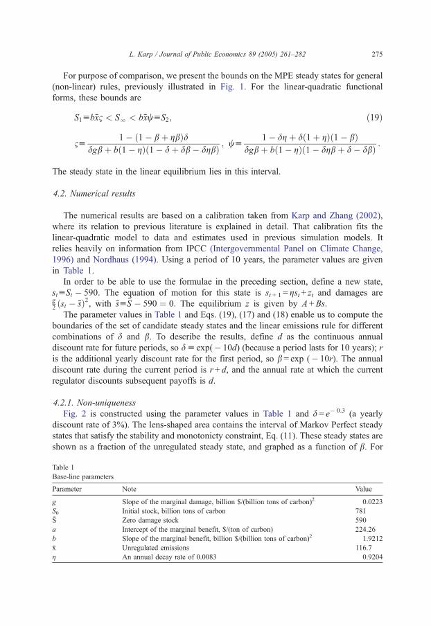
The numerical results are based on a calibration taken from Karp and Zhang (2002),

where its relation to previous literature is explained in detail. That calibration fits the

linear-quadratic model to data and estimates used in previous simulation models. It

relies heavily on information from IPCC (Intergovernmental Panel on Climate Change,

1996) and Nordhaus (1994). Using a period of 10 years, the parameter values are given

in Table 1.

In order to be able to use the formulae in the preceding section, define a new state,

stuSt � 590. The equation of motion for this state is st + 1 = gst+ zt and damages areg2ðst � sÞ2, with suS � 590 ¼ 0. The equilibrium z is given by A +Bs.

The parameter values in Table 1 and Eqs. (19), (17) and (18) enable us to compute the

boundaries of the set of candidate steady states and the linear emissions rule for different

combinations of d and b. To describe the results, define d as the continuous annual

discount rate for future periods, so du exp(� 10d) (because a period lasts for 10 years); r

is the additional yearly discount rate for the first period, so b = exp (� 10r). The annual

discount rate during the current period is r + d, and the annual rate at which the current

regulator discounts subsequent payoffs is d.

4.2.1. Non-uniqueness

Fig. 2 is constructed using the parameter values in Table 1 and d = e� 0.3 (a yearly

discount rate of 3%). The lens-shaped area contains the interval of Markov Perfect steady

states that satisfy the stability and monotonicty constraint, Eq. (11). These steady states are

shown as a fraction of the unregulated steady state, and graphed as a function of b. For

Table 1

Base-line parameters

Parameter Note Value

g Slope of the marginal damage, billion $/(billion tons of carbon)2 0.0223

S0 Initial stock, billion tons of carbon 781

S Zero damage stock 590

a Intercept of the marginal benefit, $/(ton of carbon) 224.26

b Slope of the marginal benefit, billion $/(billion tons of carbon)2 1.9212

x Unregulated emissions 116.7

g An annual decay rate of 0.0083 0.9204

Fig. 2. Ratio of regulated to unregulated steady states. The lens is the set of (stable, monotonic) MPE and the

dotted curve is the linear MPE.


example, for b = e� 0.2 = 0.82 (a yearly discount rate of 2%), the ratio between the MPE

steady state and the unregulated steady state ranges from 0.84 to 0.88. For b = 0 there is no

regulation, and for b = 1 there is constant discounting. For both of those cases, there is a

unique equilibrium.

The dotted curve shows the ratio between the steady state in the linear equilibrium and

the unregulated steady state as a function of b. The linear equilibrium achieves nearly the

lowest steady state stock that is feasible in a MPE. In view of Proposition 3, this fact

means that the linear equilibrium is ‘‘close to’’ the Pareto dominant MPE. For example, for

b = 0.82, the ratio of steady states in the linear and unregulated equilibria is 0.846, only

0.6% higher than in the lowest MPE steady state (and 4% smaller than the largest MPE

steady state). In addition, the linear equilibrium is defined over the entire real line; as noted

in Section 3.3.1, the domain of other (non-linear) equilibria is unknown.

4.2.2. The short and medium run

Table 2 shows the short and medium term effects of different combinations of d (the

columns) and r (the rows) in the linear equilibrium. The first element of each entry is the

percentage reduction in emissions during the first period, relative to the BAU emissions.

The second element is the percentage reduction of the stock after 10 periods (100 years),

relative to the BAU level.

Table 2

First element of each entry: the first period percentage abatement; second element: percentage reduction in stock

after 10 periods

r\d 0.01 0.03 0.05 0.07

0 (25.1, 18.4) (9.8, 8.8) (5.2, 5.2) (3.3, 3.5)

0.02 (20.8, 15.6) (8.1, 7.3) (4.3, 4.3) (2.7, 2.9)

0.04 (17.4, 13.2) (6.7, 6.1) (3.5, 3.6) (2.2, 2.4)


The first row of the table shows these two values for four levels of d when the regulator

has a constant discount rate (r = 0). Higher discounting leads to a drop in abatement since

the costs of abatement are borne in the current period and the benefits arise from lower

environmental damages in the future. Beginning with d = 0.01, an increase in the discount

rate causes a substantial fall in abatement. For example, with r = 0, an increase in the

constant discount rate from d = 0.01 to d = 0.03 reduces first period abatement from about

25% of the BAU level to approximately 10%, a large change. A further increase in the

discount rate to d = 0.05 causes abatement to fall by an additional 50%.

It is instructive to compare the sensitivity of the results to different parameter changes.

For example, if we fix d = 0.03, r = 0 but triple the estimate of damages (multiply g by 3),

the first period abatement increases to 25.5% and the stock reduction (relative to the BAU

level) after 100 years increases to 20.7%. In other words, beginning with our baseline

parameters and d = 0.03, r = 0, a reduction in the annual discount rate to 0.01 has

approximately the same effect on policies as does a tripling of the estimate of damages.

These results illustrate the two problems associated with constant discounting in

determining policies to control long-lived environmental problems: The optimal policies

tend to be very sensitive to the discount rate, and for reasonable discount rates the

regulator may be unwilling to bear moderate costs today in order to prevent substantial

damages in the distant future.

The last two rows show the effect of hyperbolic discounting. As expected, this

discounting reduces abatement. Perhaps the most interesting result is that the magnitude

of this change is moderate. When d = 0.01 and r = 0.02, the annual discount rate during the

first 10 year period is 0.03; subsequent payoffs are discounted at the rate of 0.01 per year.

Holding d = 0.01 and increasing r from 0 to 0.02 causes first period abatement to fall from

approximately 25% to 21%, a moderate change.

Compare the following two changes. In the first, we change the parameters from

d = 0.01, r = 0 to d = 0.03, r = 0 and in the second, we change the parameters from d = 0.01,

r = 0 to d = 0.01, r= 0.02, These two changes have the same effect on the discount rate

during the first 10 year period—it changes from 1 to 3%—but they obviously have

different effects on the discounting applied to subsequent periods. The first change causes

a large reduction in the level of abatement, and the second causes a moderate reduction.

These numerical experiments suggest that the optimal control of greenhouse gasses

may be relatively insensitive to the discount rate for the near future, holding fixed the

discounting between periods in the distant future. In addition, the regulator may be willing

to incur substantial abatement costs even if the short-term discount factor is non-

negligible, provided that the long-term discount factor is small.

5. Conclusion

There is a strong argument for discounting the future, but the use of a constant discount

rate has unfortunate implications for models of long-lived environmental problems. The

optimal policy is likely to be sensitive to the choice of the discount rate, and moderate

discounting makes us unwilling to incur even moderate costs today to avoid large damages

in the distant future.


Hyperbolic discounting is a plausible description of how people think about trading-off

costs and benefits in the distant future. It also may ameliorate some of the modeling

defects of constant discounting. Numerical examples show that if the inter-period discount

rate used for distant events is held constant, equilibrium policies are relatively insensitive

to the discount rate applied to events in the near future. In addition, in equilibrium, a

planner with a relatively large near-term discount rate may be willing to incur substantial

costs to protect the future.

The time-inconsistency problem is an integral aspect of hyperbolic discounting.

Dynamic environmental models can incorporate this feature, rather than assuming it away

by allowing the current regulator to commit. Although the resulting equilibria are non-

unique, they have a simple Pareto ranking, at least in the neighborhood of the steady state.

The linear-quadratic model is particularly useful in this context, because the linear

equilibrium exists for all state space and it can be analyzed so easily; in addition,

examples show that it is close to the Pareto dominant MPE.

Optimal control methods have been used to study a wide range of stock-related

environmental issues. Many of these same issues can also be studied in the (arguably)

more realistic situation where the regulator uses hyperbolic discounting and cannot

commit to future actions.

Acknowledgements

This paper benefited from comments from Partha Dasgupta, Geoffrey Heal, Cameron

Hepburn, Martin Weitzman, seminar participants at Arizona State University, the

participants at the 2003 EAERE conference in Bilbao and four anonymous referees.

The usual disclaimer applies.

Appendix A. Derivations and Proof

Derivation of Eq. (5).

Suppose that ‘‘Regulator t’’ believes that all subsequent regulators will use the control

rule z = v(S). In this case, the present value of Regulator t’s equilibrium continuation

payoff from time t + 1 onwards is a function V(St + 1) that satisfies the recursive relation

V ðStþ1Þ ¼ ½hðStþ1; vðStþ1ÞÞ þ dV ðgStþ1 þ vðStþ1ÞÞ�: ð20Þ

Since Regulator t treats the function v as given, she takes the function V as given.

Regulator t solves the following dynamic optimization problem

W ðStÞ ¼ maxz

½hðSt; zÞ þ bdV ðgSt þ zÞ�: ð21Þ

Recall that Regulator t discounts next period’s payoff using the factor bd. A necessary

condition for the function v to be a stationary Markov Perfect Nash equilibrium in this

game is that it solves the dynamic programming problem in (21); v must maximize the


right side of Eq. (21). We obtain the equilibrium value function by substituting the

equilibrium control rule into Eq. (21), giving

W ðStÞ ¼ ½hðSt; vðStÞÞ þ bdV ðgSt þ vðStÞÞ�: ð22Þ

Regulator t understands that Regulator t + 1 solves an analogous control problem,

possibly with a different value of the initial state, S. Thus, the value function W(St + 1) also

satisfies Eq. (22) with t replaced by t + 1. Using Eqs. (20) and (22), and defining

H(St)u h (St, v(St)) we have

bdV ðStþ1Þ ¼ d½W ðStþ1Þ � HðStþ1Þð1� bÞ�: ð23Þ

Substituting Eq. (23) into Eq. (21) we obtain the dynamic programming Eq. (5).

Derivation of Eq. (7).

We first use the envelope theorem and Eq. (5) and rearrange to obtain

WVðStÞ � fhSðSt; ztÞ � dð1� bÞgHSðStþ1Þg ¼ dgWVðStþ1Þ: ð24Þ

Rearranging Eq. (6) and multiplying both sides of the resulting equation by g gives

�fhzðSt; ztÞ � dHSðStþ1Þð1� bÞgg ¼ dgWVðStþ1Þ: ð25Þ

These two equations imply WV(St)={hS (St, zt)� hz(St, zt)g}. Advancing this equation by

1 period and substituting the result into Eq. (6) implies

hzðSt; zÞ ¼ �fd½hsðStþ1; ztþ1Þ � hzðStþ1; ztþ1Þg � HSðStþ1Þð1� bÞ�g: ð26Þ

Use the definition of H() to write HS(S) = hS (S, v (S)) + hz (S, v (S))vV(S). Substitutingthis expression into Eq. (26) and simplifying yields Eq. (7).

Proof of Proposition 1.We begin with some definitions to ease the notation and then prove

the proposition. Define the value of the next period stock, given current stock S and current

emissions z, as yu gS+ z. By Eq. (2) St + 1 = yt. With this definition, the continuation payoff

in the maximand of the DPE (5) can be written as {d [W(St + 1)�H(St + 1)(1� b)]}={d[W( yt )�H( yt )(1� b)]}uU( yt ).

The single period payoff, written in terms of y, is k (S, y)u h (S, z) from which we obtain

kS +gky = hS, kSy + gkyy = hSz kyy = hzz, which implies kSy=(hSz� ghzz). Thus, we have the

following relation

kSyz0ZðhSz � ghzzÞz0: ð27Þ

Define the equilibrium value of y(S) as w(S)u S+ v (S). The stock is non-decreasing if

wV(S)z 0; the stock is non-increasing if wV(S)V 0.

Proof. (Proposition 1) Consider two arbitrary stock levels, S*>S**, and let y**=w (S**)

be the corresponding optimal levels of y. By optimality,

kðS*; y*Þ þ Uðy�ÞzkðS*; y**Þ þ Uðy**Þ

kðS**; y**Þ þ Uðy**ÞzkðS**; y*Þ þ Uðy*Þ:


Adding these two equations implies

0VkðS*; y*Þ�kðS*; y**ÞþkðS**; y**Þ�kðS**; y*Þ ¼Z S

S**

* Z y

y**

*A2kðS; yÞASAy

dydS

ð28Þ

If Eq. (8) holds, then kSyz 0 by Eq. (27), so y*z y** by Eq. (28). If Eq. (9) holds, the

same argument implies that y*V y**. 5

Derivation of Eqs. (17) and (18)

Substitute A +BSV into the expression for h (SV, zV) and use the equation of motion,

SV= gS + z, to write the resulting expression as a function of the current stock and

emissions. The single period payoff in the next period, as a function of the current stock

and control is

HðS; zÞuf þaðAþBðgSþ zÞÞ� 1

2bðAþBðgSþ zÞÞ2�cðgSþ zÞ� 1

2gðgSþ zÞ2:

Using the quadratic value function, the value of W in the next period is

k þ lðgS þ zÞ þ q2ðgS þ zÞ2

Using the definition e = 1� b, the dynamic programming Eq. (5) specializes to

k þ lS þ q2S2 ¼ maxzf þ az� b

2z2 � cS � g

2S2 þ dðk þ lðgS þ zÞ

þ q2ðgS þ zÞ2 � eHðS; zÞÞ: ð29Þ

The first order condition implies the control rule z =A +BS, with

A ¼ �ð�dcþ daB� dbBAÞeþ aþ dl�ðdbB2 þ dgÞeþ b� dq

ð30aÞ

B ¼ �dgðbB2 þ gÞeþ q

ðdbB2 þ dgÞe� bþ dq: ð30bÞ

Solving Eq. (30b) for q gives

q ¼ �ðdbB3 þ Bdg þ dbB2g þ dggÞeþ Bb

dðBþ gÞ : ð31Þ


Substituting the control rule into equation (29) produces the maximized DPE. Equating

coefficients in orders of S implies

l ¼ � 1

2

Veþ 2bc� 2adqg � 2gbdl � 2dcq�ðdbB2 þ dgÞeþ b� dq

ð32Þ

Xu� ð�2gbaBþ 2cg þ 2gb2BAþ 2abB2g þ 2gbcþ 2B2bcþ 2aggÞd

q ¼ � ðB2dg2b2 þ dbgg2 þ dg2 þ B2ddgÞeþ dgq þ dbqg2 � bg

ðdbB2 þ dgÞe� bþ dq: ð33Þ

Substituting the expression for q in Eq. (31) into the right side of Eq. (33) and

simplifying implies that q = bgB� g. Setting this value of q equal to the right side of Eq.

(31) implies Eq. (17). To obtain Eq. (18) we use q = bgB� g in Eq. (32) to obtain an

expression for l. Using this expression in Eq. (30a) implies Eq. (18).

References

Ainslie, G., 1991. Derivation of ‘rational’ economic behavior from hyperbolic dicount curves. American Eco-

nomic Review 81 (2), 334–340.

Arrow, K.W., Cline, K.-G., Maler, M., Munasinghe, M., Squitieri, R., Stiglitz, J., 1996. Intertemporal equity,

discounting, and economic efficiency. In: Bruce, H.L.J.P., Haites, E. (Eds.), Climate Change 1995:Economic

and Social Dimensions of Climate Change. Cambridge University Press, Cambridge, pp. 128–144.

Ausebel, L., Deneckere, R., 1989. Reputation and bargaining in the durable goods monopoly. Econometrica 57

(3), 511–532.

Blanchard, O., Fischer, S., 1990. Lectures on Macroeconomics MIT Press, Cambridge, MA.

Chari, V., Kehoe, P., 1990. Sustainable plans. Journal of Political Economy 98 (6), 783–802.

Chichilnsky, G., 1996. An axiomatic approach to sustainable development. Social Choice and Welfare 13,

231–257.

Cline, W.R., 1999. Discounting for the very long term. In: Portney, P.R., Weyant, J. (Eds.), Discounting and

Intergenerational Equity (Resources for the Future).

Cropper, M., Laibson, D., 1999. The implications of hyperbolic discounting for project evaluation. In:

Portney, P.R., Weyant, J. (Eds.), Discounting and Intergenerational Equity (Resources for the Future).

Cropper, M.L., Ayded, S.K., Portney, P.R., 1994. Preferences for life-saving programs: how the public discounts

time and age. Journal of Risk and Uncertainty 8, 243–266.

Dasgupta, P., Maler, K.-G., Barrett, S., 1999. Intergenerational equity, social discount rates and global

warming. In: Portney, P.R., Weyant, J. (Eds.), Discounting and Intergenerational Equity (Resources for

the Future).

Driskill, R., 2002. A Proposal for a Selection Criterion in a Class of Dynamic Rational Expectations Models with

Multiple Equilibria Department of Economics, Vanderbilt University.

Frederick, S., Loewenstein, F., O’Donoghue, T., 2002. Time discounting and time preference: a critical review.

Journal of Economic Literature XL, 351–401.

Gollier, C., 2002. Time horizon and the discount rate. Journal of Economic Theory 75, 229–253.

Harris, C., Laibson, D., 2001. Dynamic choices of hyperbolic consumers. Econometrica 69 (5), 935–957.

Heal, G., 1998. Valuing the Future: Economic Theory and Sustainability Columbia University Press, New York.

Heal, G., 2001. Intertemporal welfare economics and the environment. In: Maler, K.-G., Vincent, J. (Eds.), The

Handbook of Environmental Economics. North Holland, Amsterdam.


Intergovernmental Panel on Climate Change, 1995. In: Houghton, J.T., Meira Filho, L.G., Callander, B.A.,

Harris, N., Kattenberg, A., Maskell K. (Eds.). Climate Change 1995: The Science of Climate Change IPCC

(Cambridge, UK).

Karp, L., 1996. Depreciation erodes the coase conjecture. European Economic Review 40 (2), 473–490.

Karp, L., 2004. Non-constant discounting in continuous time Department of Ag and Resource Economics,

University of California, Berkeley (http://are.Berkeley.EDU/karp/).

Karp, L., Zhang, J., 2002. Regulation with Anticipated Learning about Environmental Damage Giannini Foun-

dation of Agricultural Economics, University of California, Berkeley (Working Paper No. 926; http://are.

Berkeley.EDU/karp/).

Kirby, K., Herrenstein, R., 1995. Preference reversals due to myopic discounting and delayed reward. Psychology

Science 6 (2), 83–89.

Krusell, P., Smith, A., 2003. Consumption–saving desisions with quasi-geometric discounting. Econometrica 71

(1), 365–375.

Li, C.Z., Lofgren, K.G., 2000. Renewable resources and economic sustainability: a dynamic analysis with

heterogeneous time preferences. Journal of Environmental Economics and Management 40, 236–250.

Newell, R., Pizer, W., 2003. Discounting the distant future: how much do uncertain rates increase valuations.

Journal of Environmental Economics and Management 46 (1), 52–71.

Nordhaus, W., 1994. Managing the Global Commons: The Economics of the Greenhouse Effect MIT Press,

Cambridge, MA.

Phelps, E., Pollack, R., 1968. On second-best national savings and game: equilibrium growth. Review of

Economic Studies 35, 185–199.

Rabin, M., 1998. Psychology and economics. Journal of Economic Literature 36, 11–46.

Read, D., 2001. Is time-discounting hyperbolic or subadditive? Journal of Risk and Uncertainty 23 (1), 5–32.

Rubinstein, A., 2003. Economics and psychology? The case of hyperbolic discounting. International Economic

Review 44 (4), 1207–1216.

Strotz, R., 1956. Myopia and inconsistency in dynamic utility maximization. Review of Economic Studies 23,

165–180.

Tsutsui, S., Mino, K., 1990. Nonlinear strategies in dynamic duopolisitc competition with sticky prices. Journal

of Economic Theory 52, 136–161.

Weitzman, M., 2001. Gamma discounting. American-Economic-Review 91 (1), 260–271.

http://are.Berkeley.EDU/karp/

http://are.Berkeley.EDU/karp/

Date post:	07-Apr-2018
Category:	Documents
Upload:	buikien
View:	219 times
Download:	4 times

Global warming and hyperbolic discountingkarp/JpubEcon05.pdfmoderate discount rates, large future...

Documents